Modelling modal gating of ion channels with hierarchical Markov models

Abstract.

Many ion channels spontaneously switch between different levels of activity. Although this behaviour known as modal gating has been observed for a long time it is currently not well understood. Despite the fact that appropriately representing activity changes is essential for accurately capturing time course data from ion channels, systematic approaches for modelling modal gating are currently not available. In this paper, we develop a modular approach for building such a model in an iterative process. First, stochastic switching between modes and stochastic opening and closing within modes are represented in separate aggregated Markov models. Second, the continuous-time hierarchical Markov model, a new modelling framework proposed here, then enables us to combine these components so that in the integrated model both mode switching as well as the kinetics within modes are appropriately represented. A mathematical analysis reveals that the behaviour of the hierarchical Markov model naturally depends on the properties of its components. We also demonstrate how a hierarchical Markov model can be parameterised using experimental data and show that it provides a better representation than a previous model of the same data set. Because evidence is increasing that modal gating reflects underlying molecular properties of the channel protein, it is likely that biophysical processes are better captured by our new approach than in earlier models.

1. Introduction

Ion channels regulate the flow of ions across the cell membrane by stochastic opening and closing. As soon as it became possible to detect currents generated by the movement of charged ions through the channel via the patch-clamp technique [21], Colquhoun and Hawkes, [7] developed the theory of modelling single ion channels with continuous-time Markov models which describe the time-course of opening and closing that is reflected in single-channel currents by stochastic jumps between zero (closed) and one or more small non-zero current levels in the pA range (open). The activity of an ion channel is usually measured by its open probability $P_{O}$. But by 1983, Magleby and Pallotta, 1983b [19], Magleby and Pallotta, 1983a [18] had already observed spontaneous changes between different levels of channel activity in the calcium-activated potassium channel. Since then this phenomenon, known as modal gating, has been ubiquitously observed across a wide range of ion channels but the significance of modal gating has remained unclear.

In this study we present a general framework for building data-driven models of ion channels that account for modal gating. This is essential for accurately representing the dynamics of an ion channel—instead of producing a misleading constant intermediate open probability $P_{O}$, a model should represent the switching between highly different levels of activity characteristic of each mode. This is illustrated in Figure 1 where data points labelled M¹ form a segment characterised by a low open probability whereas, the segment labelled M² is characterised by a high open probability. In a realistic time series, the changes between M¹ and M² occur on a time scale so slow that a model fitted directly to the sequence of closed and open events would not be able to resolve this. Thus, instead of infrequent switching between high and low open probabilities, a model fitted directly to the data would show an intermediate open probability rather than switching between high and low open probabilities. On the other hand, modes of an ion channel have been associated with biophysical properties of the channel protein [26]. Therefore, a model accounting for modal gating is more likely to appropriately relate the dynamics of ion channels to underlying biophysical states of the channel protein.

Nevertheless, except for two recent models of the inositol trisphosphate receptor (IP₃R), see Ullah et al., [29], Siekmann et al., 2012b [27], modal gating is usually not considered in ion channel models. One difficulty in appropriately representing modal gating of ion channels in a model is the fact that for a time series of measurements collected from an ion channel it is impossible to infer directly in which mode the channel is at a given point in time. However, Siekmann et al., [26] have shown how this information can be obtained by statistical changepoint analysis, see Figure 1. The method identifies significant changes of the open probability between adjacent segments in time series of open and closed events recorded from an ion channel.

				$j_{n}$						$j_{n+1}$
$S^{k}$:	M1	M1	M1		M2	M2	M2	M2	M2		M1	M1
$T^{k}$:	O	C	C		O	C	O	O	O		C	C

Figure 1. After a statistical analysis of modal gating [26], changepoints $j_{n}$ have been inferred for a time series of ion channel data. Through this segmentation, the original time series $T^{k}$ of open (O) and closed (C) events has been augmented by the additional information $S^{k}$ of the mode (M¹, M²…) that the channel is in for a given point in time.

As a result, after this analysis has been carried out, for each point in the time series it is not only known if the channel is open (O) or closed (C) but also, in which of the modes M¹, M², … the channel is. Previously, we observed stochastic switching between a nearly inactive mode M¹ and a highly active mode M² in data from the IP₃R [26]. In this paper we will represent the stochastic process of switching between an arbitrary number of different modes $\text{M}^{i}$ by a continuous-time Markov model with infinitesimal generator $\tilde{M}$. For data by Wagner and Yule, [31], empirical histograms suggest that the sojourn time distribution $f_{\text{{\color[rgb]{0,0,1}M${}^{1}$}}}(t)$ within mode M¹ is not exponential (see Figures 5 and 6 in Siekmann et al., [26] and Figure 5a). For this reason, in general, more than one state is needed for accurately representing the process of switching between modes. This means that modal sojourn times are represented by phase-type distributions, a class of distributions which is defined by the time a Markov chain spends in a set of transient states until exiting to an absorbing state [22, 23]. We assume that the infinitesimal generator $\tilde{M}$ representing the switching between modes $\text{M}^{i}$, $i=1,\dots\ n_{M}$, has the following block structure:

(1) $$\tilde{M}=\begin{pmatrix}\tilde{M}^{1,1}&|&\tilde{M}^{1,2}&|&\dots&|&\tilde{M}^{1,n_{M}}\\ \hline\cr\tilde{M}^{2,1}&|&\tilde{M}^{2,2}&|&\dots&|&\tilde{M}^{2,n_{M}}\\ \vdots&&&\ddots&&&\vdots\\ \vdots&&&&\ddots&&\vdots\\ \vdots&&&&&\ddots&\vdots\\ \tilde{M}^{n_{M},1}&|&\dots&\dots&\dots&|&\tilde{M}^{n_{M},n_{M}}\end{pmatrix},$$

where the block matrices $\tilde{M}^{i,i}\in\mathbb{R}^{m_{i}\times m_{i}}$, $m_{i}\in\mathbb{N}$, on the diagonal describe transitions between states that represent the same mode $\text{M}^{i}$ whereas the off-diagonal blocks $\tilde{M}^{i,j}\in\mathbb{R}^{m_{i}\times m_{j}}$ represent transitions between states representing different modes $\text{M}^{i}$ and $\text{M}^{j}$, $i\neq j$. An example for a model for switching between two modes M¹ and M² is shown in Figure 2a.

Our modal gating analysis illustrated in Figure 1 not only enables us to represent the stochastic process of switching between modes $\text{M}^{i}$ but by studying the dynamics within representative segments we can investigate the processes of stochastic opening and closing characteristic of each mode. For the example in Figure 1 the dynamics within mode M² can be analysed by considering the sequence of open and closed events between $j_{k}$ and $j_{k+1}$. The dynamics within a mode $\text{M}^{i}$ can be represented by a Markov model with infinitesimal generator $Q^{i}$ which is obtained by fitting to representative segments of the same mode [27]. Similar to the sojourn times in the modes $\text{M}^{i}$, the open and closed time distributions $f_{O}(t)$ and $f_{C}(t)$, respectively, are non-exponential and more than one open or closed state may be needed for accurately representing the dynamics. For the example shown in Figure 1 we obtain two models with infinitesimal generators $Q^{1}$ and $Q^{2}$, see Figure 2b.

In this paper we develop a new mathematical model, the continuous-time hierarchical Markov model, that accounts simultaneously for both transitions between modes as well as the stochastic opening and closing within modes. Whereas a hierarchical Markov model in discrete time has been previously described [8] we are not aware of a continuous-time version discussed in the literature, so we develop the mathematical theory in detail and prove some fundamental properties. For the example of modal gating we assume that switching between modes $\text{M}^{i}$ is a top-level process that regulates the bottom-level process, the opening and closing of the channel characteristic of a particular mode $\text{M}^{i}$. This is illustrated in Figure 2.

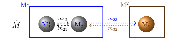
(a) inter-modal transitions

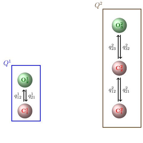
(b) intra-modal dynamics

Figure 2. Modular components of a model for modal gating. (a) gives an example for an aggregated Markov model $\tilde{M}$ representing inter-modal dynamics, the stochastic switching between two modes, M¹ and M². M¹ is modelled by an aggregate of two states whereas M² is represented by one state. The rates $m_{23}$ and $m_{32}$ stand for transitions between both modes. Note that $\tilde{M}$ may in general represent transitions between more than two modes, therefore the states $\tilde{M}^{i}_{j}$ are numbered consecutively by subscripts $j$ whereas the superscripts $i$ indicate the mode $\text{M}^{i}$. (b) shows models $Q^{1}$ and $Q^{2}$ representing the stochastic opening and closing that is characteristic of mode M¹ or M², respectively. The states $C^{i}_{k}$ and $O^{i}_{k}$ are numbered similarly to the $\tilde{M}^{i}_{j}$. Note that $k=1,\dots,n_{i}$ for each mode $\text{M}^{i}$ in contrast to the states $\tilde{M}^{i}_{j}$ where the index $j$ runs from 1 to the total number of states. In Figure 3 we show how $\tilde{M}$ and the $Q^{i}$s are combined in a model that accurately represents both inter-modal transitions as well as intra-modal kinetics.

The states $\tilde{M}^{i}_{j}$ are numbered consecutively by subscripts $j$ whereas the superscripts $i$ indicate the mode $\text{M}^{i}$. While the model is in mode M¹or analogously within one of the states $\tilde{M}^{1}_{1}$ or $\tilde{M}^{1}_{2}$ (Figure 2a), its opening and closing is described by the infinitesimal generator $Q^{1}$ (Figure 2b). As soon as M¹ is left to state $\tilde{M}^{2}_{3}$, the current state of model $Q^{1}$ is vacated and a state of model $Q^{2}$ is entered. Now, opening and closing is accounted for by $Q^{2}$ until the state $\tilde{M}^{2}_{3}$ and mode M² is left and state $\tilde{M}^{1}_{2}$ is entered.

The transitions between modes described via $\tilde{M}$ and the dynamics within modes captured by $Q^{i}$ illustrated in Figure 2 can be represented in a Markov model with infinitesimal generator $M$ that is derived from the individual components $\tilde{M}$ and $Q^{i}$. The idea is illustrated in Figure 3 and developed formally in Section 2.

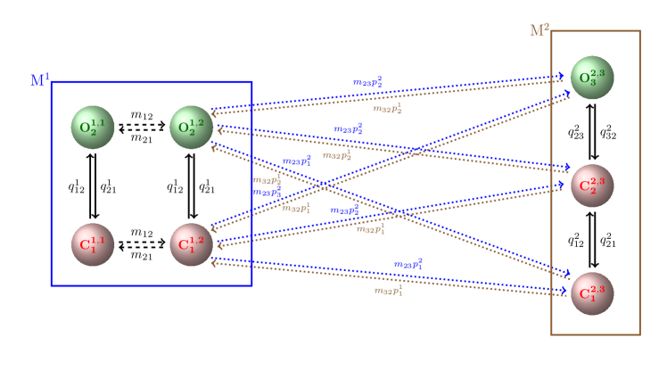
Figure 3. Aggregated Markov model that represents both transitions between modes M¹ and M² according to model $\tilde{M}$ (Figure 2a) as well as stochastic opening and closing consistent with models $Q^{1}$ and $Q^{2}$ (Figure 2b). The open and closed states are $O^{i,j}_{k}$ and $C^{i,j}_{k}$, respectively, where the superscripts $i$,$j$ refer to the state $\tilde{M}^{i}_{j}$ in the model shown in Figure 2a whereas the subscript $k$ is the index of the state within a model $Q^{i}$ shown in Figure 2b. This illustrates that the state set of the full model is obtained by the Cartesian product of states representing the modes $\text{M}^{i}$ with the states of the model $Q^{i}$. Due to the transitions $m_{12}$ and $m_{21}$ between the two states representing M¹, in the full model there are two copies of model $Q^{1}$ connected by transition rates $m_{12}$ and $m_{21}$. For transitions between modes, the rates $m_{23}$ exiting M¹ and $m_{32}$ exiting M² are weighted with stochastic vectors $p^{1}=(p^{1}_{1},p^{1}_{2})$ and $p^{2}=(p^{2}_{1},p^{2}_{2},p^{2}_{3})$ that can be interpreted as initial distributions when entering M¹ or M².

In order to account for the states $\tilde{M}^{i}_{j}$ as well as the states $O^{i}_{k}$ and $C^{i}_{k}$ representing the opening and closing within $\text{M}^{i}$, the state space of the full model consists of the Cartesian products of the $\tilde{M}^{i}_{j}$ with the $O^{i}_{k}$ and $C^{i}_{k}$. Thus, the state space of the full model consists of open and closed states $O^{i,j}_{k}$ and $C^{i,j}_{k}$, respectively, where the superscripts $i$,$j$ refer to the state $\tilde{M}^{i}_{j}$ in the model shown in Figure 2a whereas the subscript $k$ is the index of the state within a model $Q^{i}$ shown in Figure 2b. For the example shown in the figure, the closed states $C^{1,1}_{1}$ and $C^{1,2}_{1}$ as well as the open states $O^{1,1}_{2}$ and $O^{1,2}_{2}$ are connected by the transition rates $m_{12}$ and $m_{21}$. Because M¹ is modelled by two states $\tilde{M}^{1}_{1}$ and $\tilde{M}^{1}_{2}$, two “copies” of $Q^{1}$ appear in the full model whereas there is only one “copy” of $Q^{2}$ which is represented by only one state in $\tilde{M}$. For transitions between modes, the rates $m_{23}$ exiting M¹ and $m_{32}$ exiting M² are weighted with stochastic vectors $p^{1}=(p^{1}_{1},p^{1}_{2})$ and $p^{2}=(p^{2}_{1},p^{2}_{2},p^{2}_{3})$ that can be interpreted as initial distributions when entering M¹ or M². The mathematical details of the construction of this model are presented in Section 2.

It is a strength of our approach that it enables us to build data-driven models of modal gating in a modular way. After segmenting ion channel data with the method by Siekmann et al., [26] we obtain a stochastic sequence of events $\text{M}^{i}$ that describes the time course of transitions between different modes. The infinitesimal generators $\tilde{M}$ and the $Q^{i}$ can then be parameterised from these data. We demonstrate the practical implementation of this approach in Section 3 using experimental data by Wagner and Yule, [31] and compare the results with our previously published model of the same data set [27].

We investigate the mathematical structure of the continuous-time hierarchical Markov model in more detail in Section 4. In particular we show that many important properties of the infinitesimal generator $M$ of the full model can be derived from the generators $\tilde{M}$ and $Q^{i}$. We expect that similar to its discrete-time counterpart [8], the continuous-time hierarchical Markov model will have a variety of applications beyond the modelling of modal gating considered here.

We discuss our approach to modal gating in Section 5. In particular we explain why our new modelling framework is not only a better representation of ion channel dynamics but also more likely than other modelling approaches to provide a structure that realistically captures biophysical processes.

2. Methods

2.1. Preliminaries

We now develop formally the hierarchical Markov model illustrated graphically in Figures 2 and 3. First, let us describe the structure of the probability distribution $p$ over the states of the hierarchical Markov model. Let $v=(v^{1};v^{2};\dots;v^{n_{M}})$ denote a state probability distribution of the model $\tilde{M}$. That is, for $i=1,\dots,n_{M}$, $v^{i}$ is the probability distribution of the states in mode $\text{M}^{i}$. In general, we will allow $\tilde{M}$ to be an aggregated Markov model so that each of the components $v^{i}$ of the vector $v$ may itself be a vector. We make the convention that components $v^{i}$ and $v^{j}$ that are meant to refer to a vector are separated by semicolons, whereas components of a vector are separated by commas. Let us first assume for simplicity that all modes $\text{M}^{i}$ are represented by only one state so that the components $v^{i}$ are scalars. Then the distribution $p$ over the states of the full model $M$ is a weighting of the distributions $w^{i}$ over the distributions over the states of the models $Q^{i}$. Thus, we obtain $p:=(v^{1}\cdot w^{1};\dots;v^{i}\cdot w^{i};\dots;v^{n_{M}}\cdot w^{n_{M}})$. Here ‘$\cdot$’ denotes scalar multiplication of vectors $w^{i}$ with scalars $v^{i}$. If more than one state is needed for representing the modes $\text{M}^{i}$ we must generalise appropriately the “weighting” of a vector $w^{i}$ with a vector $v^{i}$. Such a generalisation is provided by the tensor product ‘$\otimes$’.

Definition 2.1 (Kronecker product $\otimes$).

We will only need the special case of the tensor product for matrices, the Kronecker product. Let $A\in\mathbb{R}^{m\times n}$, $B\in\mathbb{R}^{p\times r}$. Then

(2) $$A\otimes B:=(a_{ij}\cdot B)_{1\leq i\leq m,1\leq j\leq n}=\begin{pmatrix}a_{11}B&\dots&a_{1n}B\\ \vdots&\ddots&\vdots\\ a_{m1}B&\dots&a_{mn}B\end{pmatrix}\in\mathbb{R}^{mp\times nr}.$$

The Kronecker product also applies to vectors by identifying column vectors with $(m\times 1)$- and row vectors with $(1\times m)$-matrices.

Definition 2.2 (Kronecker sum $\oplus$).

The Kronecker sum of square matrices $A\in\mathbb{R}^{m\times m}$ and $B\in\mathbb{R}^{n\times n}$ is

(3) $$A\oplus B:=A\otimes\operatorname{id}_{n}+\operatorname{id}_{m}\otimes B\in\mathbb{R}^{mn\times mn},$$

where $\operatorname{id}_{m}$ and $\operatorname{id}_{n}$ are the identity matrices of the respective dimensions.

For some properties of Kronecker product and sum that we require for our analysis of the hierarchical Markov model (Section 4) we refer to Appendix A. For a distribution $v$ over the states of an aggregated Markov model, subvectors that represent the distributions over the states of the same mode $\text{M}^{i}$ can be naturally described by partitions.

Definition 2.3 (Partitioned vectors, multi-indices).

A multi-index is any vector $\boldsymbol{\alpha}=(\alpha_{1},\dots,\alpha_{d})\in\mathbb{N}^{d}$. We define the absolute value $|\boldsymbol{\alpha}|=\sum_{i=1}^{d}\alpha_{i}$ and denote $\dim(\boldsymbol{\alpha})=d$ the dimension of $\boldsymbol{\alpha}$.
A vector $v$ is partitioned by a multi-index $\boldsymbol{\alpha}$ if

$$v_{\boldsymbol{\alpha}}:=(v^{1};\dots;v^{i};\dots;v^{\dim(\boldsymbol{\alpha})})$$

and for each $i$ we have $v^{i}\in\mathbb{R}^{\alpha_{i}}$.
Selection of the $i$-th partition of $v_{\boldsymbol{\alpha}}$ is written as

$$v_{\boldsymbol{\alpha}}(i)=v^{i}.$$

The vector space of $\boldsymbol{\alpha}$-partitioned vectors $v_{\boldsymbol{\alpha}}$ is denoted $\mathbb{R}^{\boldsymbol{\alpha}}$.

How distributions $p$ over the states of a hierarchical Markov model relate to distributions over the states of $\tilde{M}$ and $Q^{i}$ can be clarified by the tensor product of partitioned vector spaces.

Definition 2.4 (Tensor product $\mathbb{R}^{\boldsymbol{m}}\otimes_{\boldsymbol{m},\boldsymbol{n}}\mathbb{R}^{\boldsymbol{n}}$ of $d$-partitioned vector spaces).

Let $\boldsymbol{m},\boldsymbol{n}\in\mathbb{N}^{d}$, $v_{\boldsymbol{m}}\in\mathbb{R}^{\boldsymbol{m}}$, $w_{\boldsymbol{n}}\in\mathbb{R}^{\boldsymbol{n}}$ be $d$-partitioned vectors. Then the tensor product $u_{\boldsymbol{m}\cdot\boldsymbol{n}}$ of $d$-partitioned vectors $v_{\boldsymbol{m}}$ and $w_{\boldsymbol{n}}$ is defined by

(4) $$u_{\boldsymbol{m}\cdot\boldsymbol{n}}:=v_{\boldsymbol{m}}\otimes_{\boldsymbol{m},\boldsymbol{n}}w_{\boldsymbol{n}}:=(v^{1}\otimes w^{1};\dots;v^{i}\otimes w^{i};\dots;v^{d}\otimes w^{d}),$$

with the component-wise product ${\boldsymbol{m}\cdot\boldsymbol{n}}$ of $\boldsymbol{m}$ and $\boldsymbol{n}$. With the tensor product ‘$\otimes_{\boldsymbol{m},\boldsymbol{n}}$’ we obtain the vector space

$$\mathbb{R}^{\boldsymbol{m}}\otimes_{\boldsymbol{m},\boldsymbol{n}}\mathbb{R}^{\boldsymbol{n}}$$

of the $d$-partitioned vector spaces $\mathbb{R}^{\boldsymbol{m}}$ and $\mathbb{R}^{\boldsymbol{n}}$.

Remark 2.1.

We make some remarks regarding the interpretation of Definition 2.4:

• It can be easily verified that ‘$\otimes_{\boldsymbol{m},\boldsymbol{n}}$’ fulfils the properties of a tensor product on the vector space $\mathbb{R}^{\boldsymbol{m}}\otimes_{\boldsymbol{m},\boldsymbol{n}}\mathbb{R}^{\boldsymbol{n}}$.

• Vectors $u_{\boldsymbol{m}\cdot\boldsymbol{n}}\in\mathbb{R}^{\boldsymbol{m}}\otimes_{\boldsymbol{m},\boldsymbol{n}}\mathbb{R}^{\boldsymbol{n}}$ can be written as linear combinations

  (5) $$u_{\boldsymbol{m}\cdot\boldsymbol{n}}=\sum_{k=1}^{d}\sum_{i=1}^{m_{k}}\sum_{j=1}^{n_{k}}a^{k}_{ij}(v^{k,i}_{\boldsymbol{m}}\otimes_{\boldsymbol{m},\boldsymbol{n}}w^{k,j}_{\boldsymbol{n}}),\quad a^{k}_{i,j}\in\mathbb{R}$$

  where $d=\dim{\boldsymbol{m}}=\dim{\boldsymbol{n}}$. By choosing bases $\{v^{k,i}\}$, $i=1,\dots,m_{k}$, $\{w^{k,j}\}$, $j=1,\dots,n_{k}$, we obtain systems of linearly independent vectors

  $$v^{k,i}_{\boldsymbol{m}} =(0;\dots;v^{k,i};\dots;0)\in\mathbb{R}^{\boldsymbol{m}}$$

  $$w^{k,j}_{\boldsymbol{n}} =(0;\dots;w^{k,j};\dots;0)\in\mathbb{R}^{\boldsymbol{n}}$$

  Thus, from (5) it is easy to see that

  $$\mathbb{R}^{\boldsymbol{m}}\otimes_{\boldsymbol{m},\boldsymbol{n}}\mathbb{R}^{\boldsymbol{n}}\cong\mathbb{R}^{\boldsymbol{m}\cdot\boldsymbol{n}}$$

  where ${\boldsymbol{m}\cdot\boldsymbol{n}}$ again denotes the component-wise product of $\boldsymbol{m}$ and $\boldsymbol{n}$.

2.2. A hierarchical Markov model for modal gating

Based on the block structure (1) of $\tilde{M}$ we now show how a transition matrix for the full model can be calculated from its components $\left((\tilde{m}_{0},\tilde{M}),(p^{i},Q^{i})_{i=1}^{n_{M}}\right)$. Let $\boldsymbol{m}$ and $\boldsymbol{n}$ be the multi-indices defined above. The transitions within the modes $\text{M}^{i}$ are represented in the full model by block matrices $M^{i,i}=\tilde{M}^{i,i}\oplus Q^{i}\in\mathbb{R}^{m_{i}n_{i}\times m_{i}n_{i}}$. It follows that $\dim M^{i,i}=m_{i}n_{i}$. Moreover, we define the matrix of initial conditions for a transition from $Q^{i}$ to $Q^{j}$ by

(6) $$P^{i,j}=u_{n_{i}}^{T}\otimes p^{j}=p^{j}\otimes u_{n_{i}}^{T},$$

where the row vector $p^{j}\in\mathbb{R}^{1\times n_{j}}$ is the initial condition for $Q^{j}$ from Definition 2.5, and $u_{n_{i}}^{T}\in\mathbb{R}^{n_{i}\times 1}$ is a column vector of ones. We observe that $P^{i,j}\in\mathbb{R}^{n_{i}\times n_{j}}$ so that, for $i\neq j$ we have $M^{i,j}=\tilde{M}^{i,j}\otimes P^{i,j}\in\mathbb{R}^{m_{i}n_{i}\times m_{j}n_{j}}$. We can now define the components of a continuous-time hierarchical Markov model and calculate its infinitesimal generator:

Analogous to the discrete-time hierarchical Markov model by Fine et al., [8], we define a continuous-time hierarchical Markov model.

Definition 2.5 (Components of a continuous-time hierarchical Markov model).

A continuous-time hierarchical Markov model (with a two-level hierarchy) is specified by the components $\left((\tilde{m}_{0},\tilde{M}),(p^{i},Q^{i})_{i=1}^{n_{M}}\right)$:

• An infinitesimal generator $\tilde{M}$ of a Markov model with initial distribution $\tilde{m}_{0}$ with aggregates of states $\text{M}^{i}$, $i=1,\dots,n_{M}$. The $\text{M}^{i}$ are referred to as modes.

• For each mode a Markov model with infinitesimal generator $Q^{i}$ and initial distribution $p^{i}$.

Then the infinitesimal generator $M$ of the aggregated model for modal gating is calculated as follows:

(7) $$M=\begin{pmatrix}\tilde{M}^{1,1}\oplus Q^{1}&|&\tilde{M}^{1,2}\otimes P^{1,2}&|&\dots&|&\tilde{M}^{1,n_{M}}\otimes P^{1,n_{M}}\\ \hline\cr\tilde{M}^{2,1}\otimes P^{2,1}&|&\tilde{M}^{2,2}\oplus Q^{2}&|&\dots&|&\tilde{M}^{2,n_{M}}\otimes P^{2,n_{M}}\\ \vdots&&&\ddots&&&\vdots\\ \vdots&&&&\ddots&&\vdots\\ \vdots&&&&&\ddots&\vdots\\ \tilde{M}^{n_{M},1}\otimes P^{n_{M},1}&|&\dots&\dots&\dots&|&\tilde{M}^{n_{M},n_{M}}\oplus Q^{n_{M}}\end{pmatrix}.$$

It is straightforward to generalise this definition recursively to an arbitrary number of hierarchies. From Definition 2.4 and (4) we know that an arbitrary distribution $p$ over the states of the full model can be represented by a linear combination of tensor products of the form (4). We now require for initial distributions that they should arise from a single tensor product of initial distributions over the states of $\tilde{M}$ and initial distributions over the states of the $Q^{i}$.

Definition 2.6 (Initial distribution over the states of a hierarchical Markov model).

Let $v_{\boldsymbol{m}}$ be the initial distribution over the states of the top-level model $\tilde{M}$ and $w_{\boldsymbol{n}}$, a vector whose components $w^{i}$ are initial distributions over the states of the models $Q^{i}$. Then the initial distribution $p^{0}_{\boldsymbol{m}\cdot\boldsymbol{n}}$ over the states of the full model $M$ is calculated by the tensor product ‘$\otimes_{\boldsymbol{m},\boldsymbol{n}}$’ introduced in Definition 2.4:

(8) $$p^{0}_{\boldsymbol{m}\cdot\boldsymbol{n}}=v_{\boldsymbol{m}}\otimes_{\boldsymbol{m},\boldsymbol{n}}w_{\boldsymbol{n}}=(v^{1}\otimes w^{1};\dots;v^{i}\otimes w^{i};\dots;v^{n_{M}}\otimes w^{n_{M}}).$$

Remark 2.2.

We make some remarks regarding the interpretation of Definition 8:

• Note that whereas $v_{\boldsymbol{m}}$ is a stochastic vector, $w_{\boldsymbol{n}}$ is not. It is easy to see that $p^{0}_{\boldsymbol{m}\cdot\boldsymbol{n}}$ is a stochastic vector.

• Algebraically, Definition 8 constrains initial distributions to so-called pure tensors which can be written as a single tensor product rather than a linear combination of tensor products.

• Statistically, Definition 8 says that for the initial distribution the probabilities of being in a state $\tilde{M}^{i}_{j}$ and a state $Q^{i}_{k}$ are stochastically independent: the joint probability of being in $\tilde{M}^{i}_{j}$ and $Q^{i}_{k}$ is the product of the individual probabilities (8).

It is an interesting question if the time-dependent solution $p_{\boldsymbol{m}\cdot\boldsymbol{n}}(t)$ or the stationary distribution of the full model $M$ remain in the form $p_{\boldsymbol{m}\cdot\boldsymbol{n}}(t)=v_{\boldsymbol{m}}(t)\otimes_{\boldsymbol{m},\boldsymbol{n}}w_{\boldsymbol{n}}(t)$ for $t>0$. In fact, this is generally not the case.

Remark 2.3.

Caution: In most situations, $p_{\boldsymbol{m}\cdot\boldsymbol{n}}(t)$ cannot be written as a pure tensor $p_{\boldsymbol{m}\cdot\boldsymbol{n}}(t)=v_{\boldsymbol{m}}(t)\otimes_{\boldsymbol{m},\boldsymbol{n}}w_{\boldsymbol{n}}(t)$ for $t>0$. As discussed in Proposition 4.4 we obtain a solution $(v_{\boldsymbol{m}}(t)\otimes_{\boldsymbol{m},\boldsymbol{n}}\pi_{\boldsymbol{n}})$ for a solution $v_{\boldsymbol{m}}(t)$ of $\tilde{M}$ and a vector $\pi_{\boldsymbol{n}}$ of stationary solutions $\pi^{i}$ of $Q^{i}$ if and only if we choose initial conditions $p^{i}=\pi^{i}$ for all $Q^{i}$.

2.3. Example

As an example for the construction of the infinitesimal generator $M$ from the components $\left((\tilde{m}_{0},\tilde{M}),(p^{i},Q^{i})_{i=1}^{n_{M}}\right)$ we present a model that will be used in Section 3 for experimental data from the inositol trisphosphate receptor (IP₃R).

Let the infinitesimal generator for the switching between modes be

(9) $$\tilde{M}=\begin{pmatrix}-m_{13}&0&\vline&m_{13}\\ 0&-m_{23}&\vline&m_{23}\\ \hline\cr m_{31}&m_{32}&\vline&-m_{31}-m_{32}\end{pmatrix}$$

and the models representing the intra-modal kinetics

(10) $$Q^{1}=\begin{pmatrix}-q^{1}_{12}&q^{1}_{12}\\ q^{1}_{21}&-q^{1}_{21}\end{pmatrix}\text{ and }Q^{2}=\begin{pmatrix}-q^{2}_{12}&q^{2}_{12}&0&0\\ q^{2}_{21}&-q^{2}_{21}-q^{2}_{23}-q^{2}_{24}&q^{2}_{23}&q^{2}_{24}\\ 0&q^{2}_{32}&-q^{2}_{32}&0\\ 0&q^{2}_{42}&0&-q^{2}_{42}\end{pmatrix}$$

with initial conditions

(11) $$p^{1}=(p^{1}_{1},p^{1}_{2})\text{ and }p^{2}=(p^{2}_{1},p^{2}_{2},p^{2}_{3},p^{2}_{4}).$$

Then

$$M=\begin{pmatrix}\tilde{M}^{1,1}_{2}\oplus Q^{1}&\vline&\tilde{M}^{1,2}_{2}\otimes P^{1,2}\\ \hline\cr\tilde{M}^{2,1}_{2}\otimes P^{2,1}&\vline&\tilde{M}^{2,2}_{2}\oplus Q^{2}\end{pmatrix}$$

(12) $$=\left(\begin{smallmatrix}-m_{13}-q^{1}_{12}&q^{1}_{12}&0&0&\vline&m_{13}p^{2}_{1}&m_{13}p^{2}_{2}&m_{13}p^{2}_{3}&m_{13}p^{2}_{4}\\ q^{1}_{21}&-m_{13}-q^{1}_{21}&0&0&\vline&m_{13}p^{2}_{1}&m_{13}p^{2}_{2}&m_{13}p^{2}_{3}&m_{13}p^{2}_{4}\\ 0&0&-m_{23}-q^{1}_{12}&q^{1}_{12}&\vline&m_{23}p^{2}_{1}&m_{23}p^{2}_{2}&m_{23}p^{2}_{3}&m_{23}p^{2}_{4}\\ 0&0&q^{1}_{21}&-m_{23}-q^{1}_{21}&\vline&m_{23}p^{2}_{1}&m_{23}p^{2}_{2}&m_{23}p^{2}_{3}&m_{23}p^{2}_{4}\\ \hline\cr m_{31}p^{1}_{1}&m_{31}p^{1}_{2}&m_{32}p^{1}_{1}&m_{32}p^{1}_{2}&\vline&-R-q^{2}_{12}&q^{2}_{12}&0&0\\ m_{31}p^{1}_{1}&m_{31}p^{1}_{2}&m_{32}p^{1}_{1}&m_{32}p^{1}_{2}&\vline&q^{2}_{21}&-R-q^{2}_{21}-q^{2}_{23}-q^{2}_{24}&q^{2}_{23}&q^{2}_{24}\\ m_{31}p^{1}_{1}&m_{31}p^{1}_{2}&m_{32}p^{1}_{1}&m_{32}p^{1}_{2}&\vline&0&q^{2}_{32}&-R-q^{2}_{32}&0\\ m_{31}p^{1}_{1}&m_{31}p^{1}_{2}&m_{32}p^{1}_{1}&m_{32}p^{1}_{2}&\vline&0&q^{2}_{42}&0&-R-q^{2}_{42}\end{smallmatrix}\right)$$

with $R:=m_{31}+m_{32}$.

2.4. Parameterising the model with experimental data

In order to parameterise the components $\left((\tilde{m}_{0},\tilde{M}),(p^{i},Q^{i})_{i=1}^{n_{M}}\right)$ of our model, the infinitesimal generators $\tilde{M}$ and $Q^{i}$ have to be inferred from ion channel data. We assume that the original data, a sequence of current measurements recorded with a constant sampling interval $\tau$ has been statistically analysed so that it has the form of Figure 1. Then each measurement has been classified as open (O) or closed (C) and it has also been determined in which mode $\text{M}^{i}$ the channel was at this point in time. The Markov model $\tilde{M}$ is inferred from the sequence $S^{k}$ of modes $\text{M}^{i}$ whereas the models $Q^{i}$ are parameterised from sequences of $T^{k}$ that are representative of a particular mode. For example, in Figure 1, the five data points between $j_{n}$ and $j_{n+1}$ could be used for inferring the model $Q^{2}$ representing the stochastic opening and closing within mode M².

All models are parameterised with the Bayesian method developed in Siekmann et al., [28], Siekmann et al., 2012a [25]. For inferring the infinitesimal generator $\tilde{M}$ the likelihood has the form

(13) $$\mathbb{P}((S^{k})|\tilde{M})=\tilde{\mu}\cdot P_{S^{1}}\cdot\exp(\tilde{M}\tau)\cdot P_{S^{2}}\cdot...\cdot\exp(\tilde{M}\tau)\cdot P_{S^{N}}\cdot u^{T},$$

where $(S^{k})$ is a sequence of observations of modes $\text{M}^{i}$ separated by the sampling interval $\tau$, $\tilde{M}$ is the infinitesimal generator of an aggregated Markov model, $\tilde{\mu}$ is the stationary distribution of $\tilde{M}$ and $u^{T}$ is a column vector of ones. The matrices $P_{S^{k}}$ project to the states of the model that represent the mode observed at data point $k$. For example,

(14) $$P_{\text{{\color[rgb]{0,0,1}M${}^{1}$}}}=\begin{pmatrix}\operatorname{id}_{m_{1}}&\vline&0&\vline&\dots&\vline&0\\ \hline\cr 0&\vline&\dots\\ \vdots\\ 0&\vline&\dots&\vline&\dots&\vline&0\end{pmatrix}$$

with the same block structure as in (1) projects to states representing mode M¹, the other projection matrices $P_{S^{i}}$ are defined equivalently. The likelihood for inferring the infinitesimal generators $Q^{i}$ from representative segments of $T^{k}$ of open (O) and closed (C) events (Figure 1) is analogous to (13). See Siekmann et al., [28], Siekmann et al., 2012a [25] for a detailed description of the method.

3. Data-driven modelling of modal gating

Our new framework enables us to easily construct and parameterise models for modal gating following a transparent iterative process:

1. Infer the stochastic process $S^{k}$ of switching between modes $\text{M}^{i}$ (Figure 1) using the statistical method by Siekmann et al., [26].

2. Model the process $S^{k}$ of mode switching by parameterising an infinitesimal generator $\tilde{M}$ (Figure 2a).

3. From segments of $T^{k}$ representative for the opening of closing within each of the modes M¹, M², … (Figure 2b) parameterise infinitesimal generators $Q^{1}$, $Q^{2}$, …

4. Choose initial distributions $\tilde{m}_{0}$ and $p^{i}$ and combine all components $\left((\tilde{m}_{0},\tilde{M}),(p^{i},Q^{i})_{i=1}^{n_{M}}\right)$ by calculating the infinitesimal generator $M$ of the full model (Figure 3).

Inferring $\tilde{M}$ and $Q^{i}$ using the Bayesian approach briefly described in Section 2.4 ensures that the resulting model will be highly parsimonious because at each step a model with the optimal number of parameters for representing stochastic switching between modes, and opening and closing within modes, is determined. We demonstrate the practical implementation of this process using data collected by Wagner and Yule, [31] and compare the results with our previously published model of the same data set [27].

3.1. Step (i): Statistical analysis of modal gating

Previously, we have statistically analysed mode switching exhibited in the data by Wagner and Yule, [31] and found two modes, the nearly inactive mode M¹ with a very low open probability and the highly active mode M² with $P_{O}\approx 70\%$, see Siekmann et al., [26] for details. As illustrated in Figure 1 we have a stochastic sequence of events M¹ and M² that are separated by a sampling interval $\tau=$0.05\text{\,}\mathrm{ms}$$. We have results from two types of the inositol trisphosphate receptor (type I IP₃R and type II IP₃R) for various calcium concentrations (Ca²⁺), $0.01\text{\,}\mathrm{\SIUnitSymbolMicro}\mathrm{M}$, $0.05\text{\,}\mathrm{\SIUnitSymbolMicro}\mathrm{M}$ and $5\text{\,}\mathrm{\SIUnitSymbolMicro}\mathrm{M}$, at fixed concentrations of $10\text{\,}\mathrm{\SIUnitSymbolMicro}\mathrm{M}$ inositol trisphosphate (IP₃) and $5\text{\,}\mathrm{m}\mathrm{M}$ adenosine trisphosphate (ATP). Empirical histograms of the sojourn times in M¹ and M² for all except one data set indicate that whereas time spent in the active mode M² may be represented satisfactorily by one state, accurately representing sojourn times in the nearly inactive mode M¹ seems to require at least two states, see Figure 5 for an example. Whereas one state accounts for the support of the sojourn time density in mode M² (Figure 5b) the more widespread sojourn time density in mode M¹ is better approximated by two states (Figure 5a). Thus, for five of our six data sets we parameterise $\tilde{M}$ with the structure of (9). For one data set (type II IP₃R at $0.05\text{\,}\mathrm{\SIUnitSymbolMicro}\mathrm{M}$ Ca²⁺), the histograms suggests that we need a model with two states representing M¹ and two states representing M² (Figure 7). Thus, for these data we use the following infinitesimal generator:

(15) $$\tilde{M}_{\text{Type 2 IP${}_{3}${R}, $0.05\text{\,}\mathrm{\SIUnitSymbolMicro}\mathrm{M}$ Ca${}^{2+}$}}=\begin{pmatrix}-m_{12}-m_{12}&m_{12}&\vline&m_{13}&0\\ 0&-m_{24}&\vline&0&m_{24}\\ \hline\cr m_{31}&m_{32}&\vline&-m_{31}-m_{32}&0\\ 0&m_{42}&\vline&0&-m_{42}\end{pmatrix}.$$

3.2. Step (ii): Parameterising $\tilde{M}$

Fitting $\tilde{M}$ to a time series $S^{k}$ of M¹ and M² using our MCMC method [28, 25] is a challenging problem. Because in a time series of a few hundred thousand up to about a million data points the number of transitions between the two modes is only in the order of hundreds, the data from which the rate constants have to be inferred are effectively very limited—despite the large number of data points. An example of a convergence plot shown in Figure 4 demonstrates that values of the two rates, $m_{13}$ and $m_{23}$, alternate. This is due to symmetry in the model structure chosen for the model $\tilde{M}$ where the two states $M^{1}_{1}$ and $M^{1}_{2}$ can be swapped without changing the model. This effect can be removed by considering only one mode of the multi-modal posterior, in this case by considering only samples where $m_{31}$ exceeds a certain threshold. Nevertheless, even after this correction some parameters such as the rate $m_{23}$ show a high degree of uncertainty indicated by a widespread marginal distribution (Figure 4). Mean values and standard deviations of the distributions of the model parameters are summarised in Tables 1 and 2.

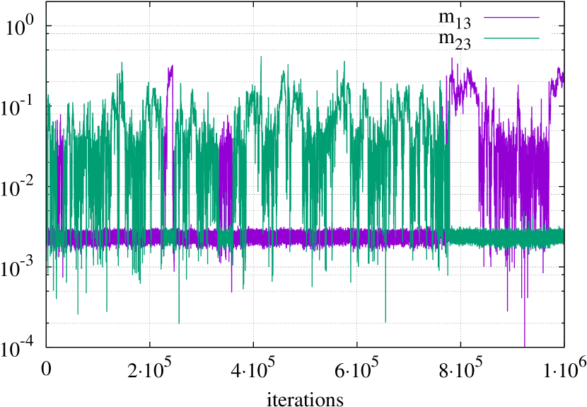
(a)

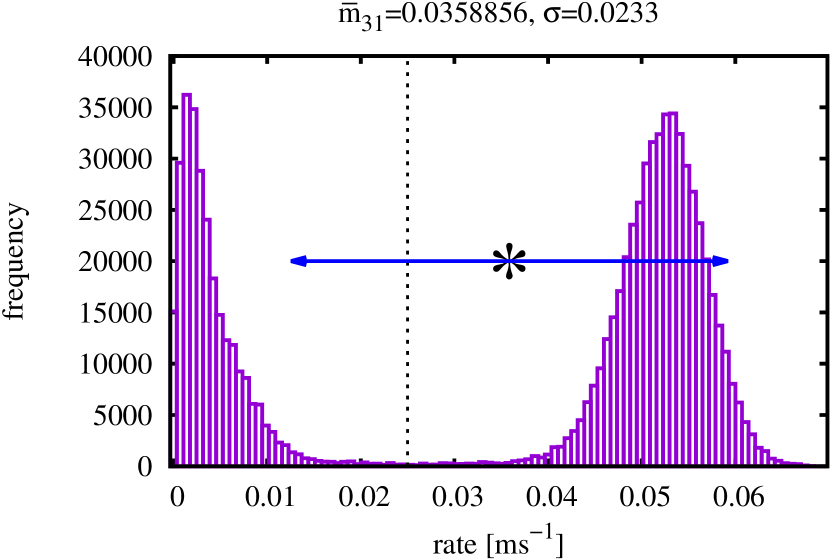
(b)

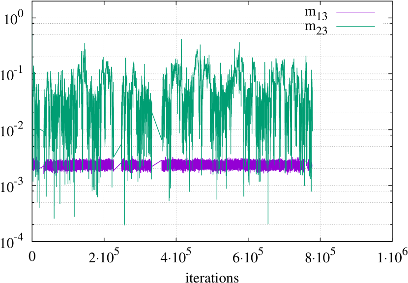
(c)

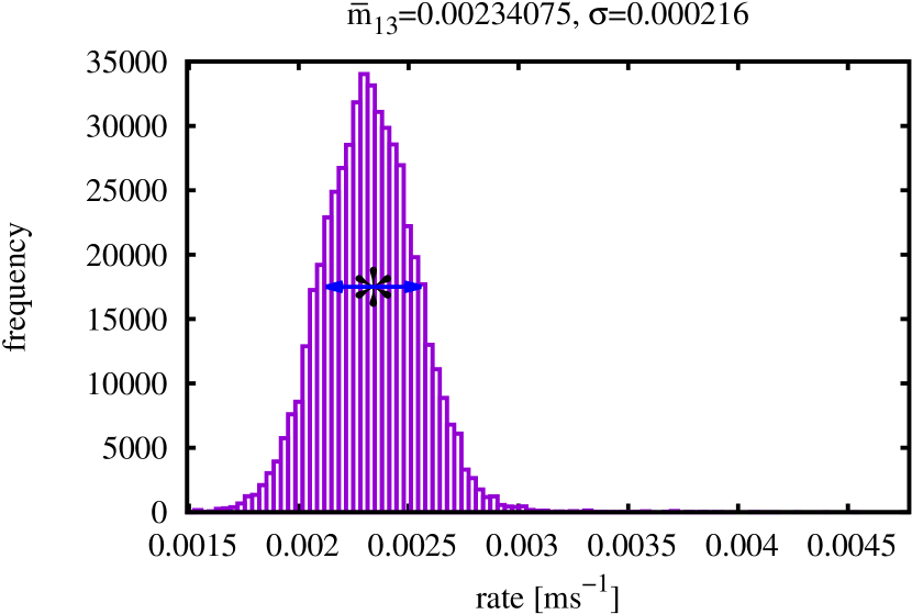
(d)

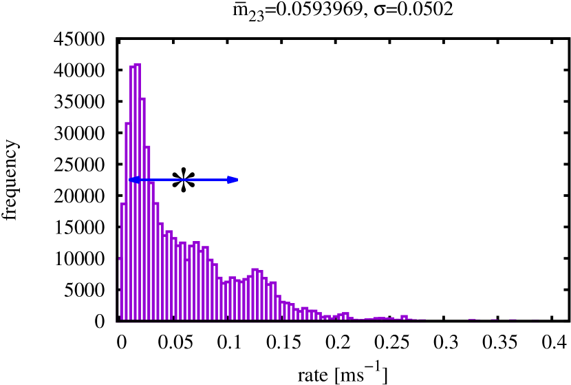
(e)

Figure 4. Fitting the stochastic transitions between modes M¹ and M² to a model $\tilde{M}$ (9) with two states representing the nearly inactive mode M¹ and one state representing the active mode M² is challenging. The MCMC sampler by Christen and Fox, [6] is run with default parameters in order to generate samples from the posterior density of the Bayesian model described in Section 2.4 [28, 25]. The convergence plot in (a) shows that over the course of $10^{6}$ iterations the samples generated for the rates that enter the state $M^{2}_{3}$ are occasionally swapped. This phenomenon is known as label switching in the MCMC literature and is caused by the symmetry of the model $\tilde{M}$ (9). The marginal histogram of the rate $m_{31}$ is bimodal with two well separated peaks (b) so that the effect of label switching can be removed by discarding samples with $m_{31}<$0.025\text{\,}\mathrm{m}\reciprocal{\mathrm{s}}$$ (indicated by a vertical line). The convergence plot obtained after thresholding is shown in (d). Whereas the marginal histogram (e) indicates that $m_{13}$ is well-constrained, the standard deviation of $m_{23}$ remains high (f). Burn-in for all histograms: $2\cdot 10^{5}$ iterations.

Type I IP3R
Ca2+[ µM]	$m_{13}$ $m_{23}$	$m_{31}$ $m_{32}$
	0.00236708 $\pm$ 0.000201138	0.0545511 $\pm$ 0.00294464
0.01	0.069589 $\pm$ 0.0510011	0.00318407 $\pm$ 0.00203495
	0.0020581 $\pm$ 0.000389371	0.0619096 $\pm$ 0.00894936
0.05	0.01873 $\pm$ 0.0111274	0.0101597 $\pm$ 0.00693104
	0.00311881 $\pm$ 0.00027425	0.0564093 $\pm$ 0.00404197
5	0.160984 $\pm$ 0.06707	0.00472598 $\pm$ 0.00189248

Table 1. Type I IP₃R: Mean values and standard deviations for the rate constants of the infinitesimal generator $\tilde{M}$ (9) in the main text representing the transitions between an inactive mode M¹ and an active mode M². All values are given in transitions per milliseconds [ m s ].

Type II IP3R
Ca2+[ µM]	$m_{13}$ $m_{23}$	$m_{31}$ $m_{32}$
	0.00134665 $\pm$ 0.000250273	0.0724154 $\pm$ 0.00817478
0.01	0.0714618 $\pm$ 0.0454381	0.0139203 $\pm$ 0.00588837
	0.00435935 $\pm$ 0.00027004	0.0284326 $\pm$ 0.00151654
5	0.146953 $\pm$ 0.0424637	0.00230764 $\pm$ 0.000712072
	$m_{12}$ $m_{13}$ $m_{24}$	$m_{21}$ $m_{31}$ $m_{42}$
	0.00112896 $\pm$ 0.000402963	0.0732717 $\pm$ 0.034058
0.05	0.000756359 $\pm$ 0.000133923	0.083959 $\pm$ 0.0184139
	0.0451628 $\pm$ 0.0168949	0.001816 $\pm$ 0.000335203

Table 2. Type II IP₃R: Mean values and standard deviations for the rate constants of the infinitesimal generator $\tilde{M}$, (9) and (15), respectively, representing the transitions between an inactive mode M¹ and an active mode M². For $0.05\text{\,}\mathrm{\SIUnitSymbolMicro}\mathrm{M}$ Ca²⁺ an additional state was required for representing the dynamics of the active mode M². All values are given in transitions per milliseconds [ m s ].

3.3. Step (iii): Parameterising $Q^{1}$ and $Q^{2}$

In our previous study Siekmann et al., 2012b [27] we have already fitted a model with two states to representative segments of the inactive mode M¹ and a model with four states for representing M², see (10) for the form of the infinitesimal generators $Q^{1}$ and $Q^{2}$. Interestingly, we could show that $Q^{1}$ and $Q^{2}$ were independent of the concentrations of IP₃, ATP and Ca²⁺. The parameter values from the Supplementary Material of Siekmann et al., 2012b [27] are reproduced here for convenience (Table 3).

	M1
	$q^{1}_{12}$	$q^{1}_{21}$
Type I IP3R	11.1 $\cdot 10^{-3}\pm$ 1.01 $\cdot 10^{-3}$	3.33 $\pm$ 0.27
Type II IP3R	4.14 $\cdot 10^{-3}\pm$ 6.7 $\cdot 10^{-4}$	3.42 $\pm$ 0.496
	M2
	$q^{2}_{12}$ $q^{2}_{23}$ $q^{2}_{24}$	$q^{2}_{21}$ $q^{2}_{32}$ $q^{2}_{42}$
	1.24 $\pm$ 0.121	0.0879 $\pm$ 0.0117
Type I IP3R	3.32 $\cdot 10^{-3}\pm$ 1.64 $\cdot 10^{-3}$	0.0694 $\pm$ 0.0266
	10.5 $\pm$ 0.0771	4.01 $\pm$ 0.0293
	1.14 $\pm$ 0.0956	0.0958 $\pm$ 0.00945
Type II IP3R	4.75 $\cdot 10^{-3}\pm$ 1.53 $\cdot 10^{-3}$	0.0119 $\pm$ 0.00357
	10.1 $\pm$ 0.0668	3.27 $\pm$ 0.0221

Table 3. Mean values and standard deviations for rate constants of the infinitesimal generators (10) representing opening and closing in M¹ and M². All values are given in transitions per milliseconds [ m s ]. Reproduced from the Supplementary Material of Siekmann et al., 2012b [27].

3.4. Step (iv): The generator $M$ of the full model

After the models $\tilde{M}$, $Q^{1}$ and $Q^{2}$ have been obtained, we finally need to specify the initial distributions $\tilde{m}_{0}$, $p^{1}$ and $p^{2}$. Consistent with the experimental assumption that recording of the data was started when the channel has reached steady state we set $\tilde{m}_{0}=\tilde{\mu}$, $p^{1}=\pi^{1}$ and $p^{2}=\pi^{2}$ where $\tilde{\mu}$, $\pi^{1}$ and $\pi^{2}$ are the stationary distributions of $\tilde{M}$, $Q^{1}$ and $Q^{2}$, respectively. After all components $\left((\tilde{m}_{0},\tilde{M}),(p^{i},Q^{i})_{i=1}^{n_{M}}\right)$ of our model have been specified, the infinitesimal generator $M$ of the full model can be calculated using (7).

3.5. Results

Due to the problems with fitting the infinitesimal generator $\tilde{M}$ (9) mentioned in Section 3.2 one may ask if a simpler two-state model representing the dynamics of modal gating would be preferable. However, the ability of a three-state model to approximate the sojourn distribution of the nearly inactive mode M¹ more accurately (Figure 5a) was found to be crucial for obtaining a better fit of the closed time distribution in comparison with the model from [27] (Figure 5c). That the model structure of the hierarchical model proposed here is better able to capture the properties of the entire time series data seems even more convincing because it has—unlike the original model from Siekmann et al., 2012b [27]— been built without directly fitting to the time series at any step of its construction.

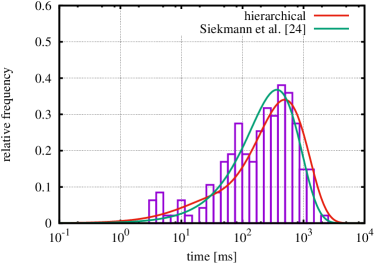
(a) sojourn time density in M¹

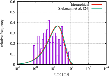
(b) sojourn time density in M²

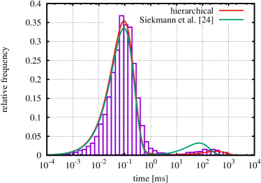
(c) closed time density

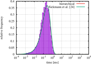
(d) open time density

Figure 5. The model from Siekmann et al., 2012b [27] and the new hierarchical model are compared for a data set from type I IP₃R for $10\text{\,}\mathrm{\SIUnitSymbolMicro}\mathrm{M}$ IP₃, $5\text{\,}\mathrm{m}\mathrm{M}$ ATP and $0.01\text{\,}\mathrm{\SIUnitSymbolMicro}\mathrm{M}$ Ca²⁺. (a) shows that the fit of the new model to the empirical sojourn time density in mode M¹ (shown in red) is slightly improved in comparison with the original model (shown in green). This improved fit of the modal kinetics clearly improves the fit to the closed time densities shown in (c).

In Figure 6 we show that the bimodal closed time distribution observed for some combinations of ligand concentrations arises due to the mixing of the closed time distributions within nearly inactive mode M¹ and active mode M² both of which only have one distinct maximum.

Figure 6. The bimodal closed time distribution (red, solid) observed for type I IP₃R for $10\text{\,}\mathrm{\SIUnitSymbolMicro}\mathrm{M}$ IP₃, $5\text{\,}\mathrm{m}\mathrm{M}$ ATP and $0.01\text{\,}\mathrm{\SIUnitSymbolMicro}\mathrm{M}$ Ca²⁺ (Figure 5c) arises due to mixing of the closed time distribution of the active mode M² (brown, dashed) and of the inactive mode M¹ (blue, dotted). Note that the mode of the closed time distribution in M¹ (blue, dotted) is shifted from about $100\text{\,}\mathrm{ms}$ to $300\text{\,}\mathrm{ms}$ in the closed time distribution of the full model. By comparison with the closed time distribution of the model from Siekmann et al., 2012b [27] (green, dash-dotted) it shows that this model is incapable of shifting the mode of the closed distribution in the nearly inactive mode M¹ to the right.

Stronger differences between both models are observed for a data set collected from type II IP₃R for $10\text{\,}\mathrm{\SIUnitSymbolMicro}\mathrm{M}$ IP₃, $5\text{\,}\mathrm{m}\mathrm{M}$ ATP and $0.05\text{\,}\mathrm{\SIUnitSymbolMicro}\mathrm{M}$ Ca²⁺. For this experimental condition, the effect of modal gating can be observed without statistical analysis (Figure 8a). Figure 7 shows that both modes M¹ and M² exhibit a widespread distribution of sojourn times which can only approximately be captured by a four-state model with two states each for both M¹ and M². Whereas the new hierarchical model can approximate the empirical distributions of both modes relatively well, the model from Siekmann et al., 2012b [27] fails due to the fact that only one characteristic sojourn time for each mode can be captured by the pair of transition rates accounting for modal gating in this model (Figure 7).

(a) sojourn time distribution in M¹

(b) sojourn time distribution in M²

Figure 7. Empirical sojourn time distributions for both modes M¹ and M² for type II IP₃R for for $10\text{\,}\mathrm{\SIUnitSymbolMicro}\mathrm{M}$ IP₃, $5\text{\,}\mathrm{m}\mathrm{M}$ ATP and $0.05\text{\,}\mathrm{\SIUnitSymbolMicro}\mathrm{M}$ Ca²⁺. Whereas the hierarchical model can resolve (by using a four-state model) the widespread distributions of both M¹ and M², the model from Siekmann et al., 2012b [27] can only capture one characteristic sojourn time due to the fact that only one pair of transition rates has been used to connect the submodels for mode M¹ and M².

Due to the failure to account for the modal sojourn time distributions, we expect the model from Siekmann et al., 2012b [27] to reproduce the kinetics observed in the data much less accurately than the new hierarchical model. In order to illustrate this we simulated both the Siekmann et al., 2012b [27] model (Figure 8c) and the new model (Figure 8b). The sample path was plotted in blue when the channel was in mode M¹ whereas it was plotted in brown when the channel was in mode M². The same colours were used for colouring the data (Figure 8a) based on the results of the statistical analysis from Siekmann et al., [26]. The comparison shows that mode switching happens much more frequently in the model from Siekmann et al., 2012b [27] than observed in the data and the proportion of relatively long sojourns is increased with respect to the data. The frequency of mode switching and the widespread distribution of sojourn lengths is better approximated by the hierarchical model. The burst of activity observed in the data starting after approximately $45\text{\,}\mathrm{s}$ is not captured by either model. This would require separate statistical analysis of the trace before and after $t=$45\text{\,}\mathrm{s}$$, the observed change of activity.

(a) data

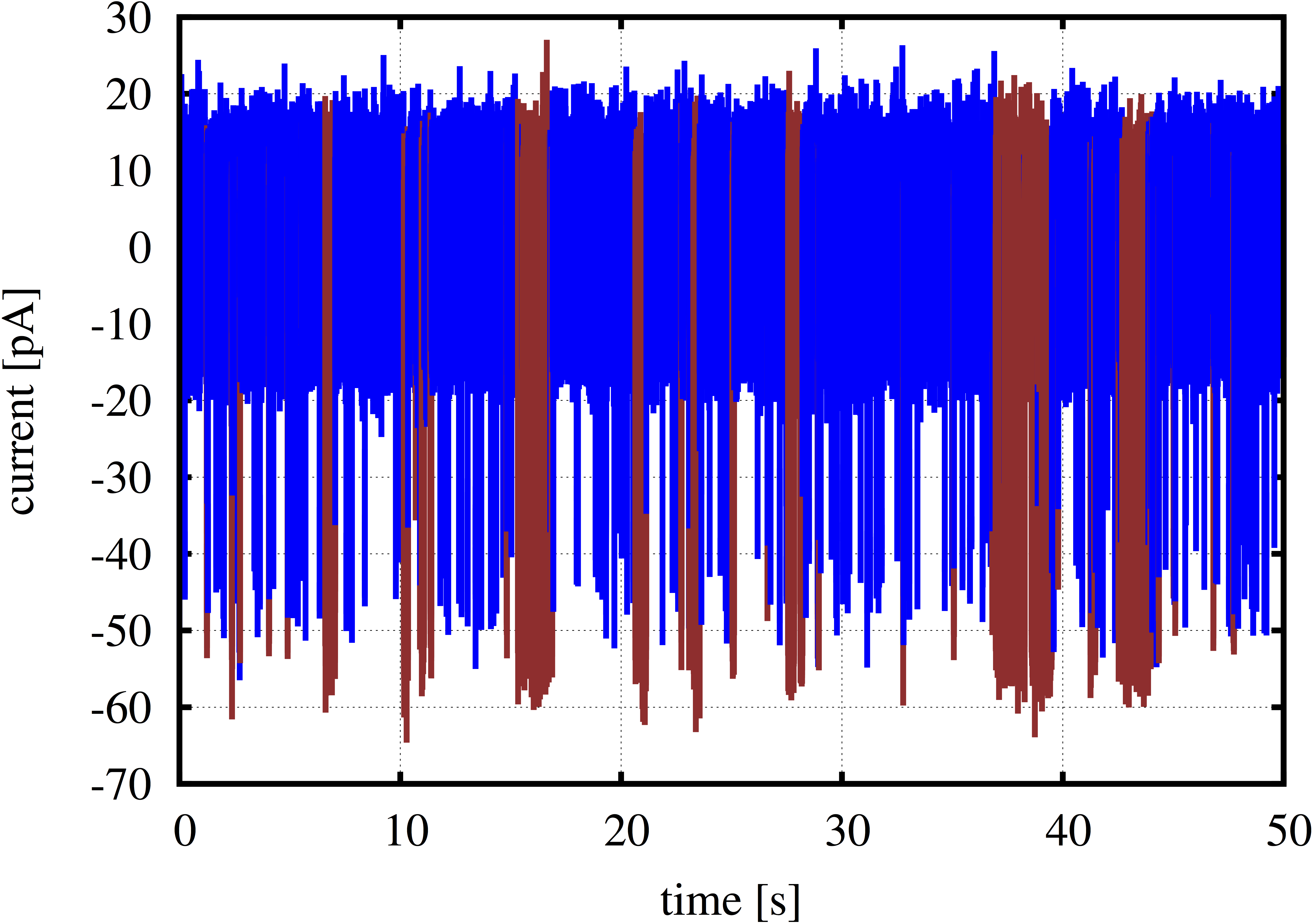
(b) Hierarchical model

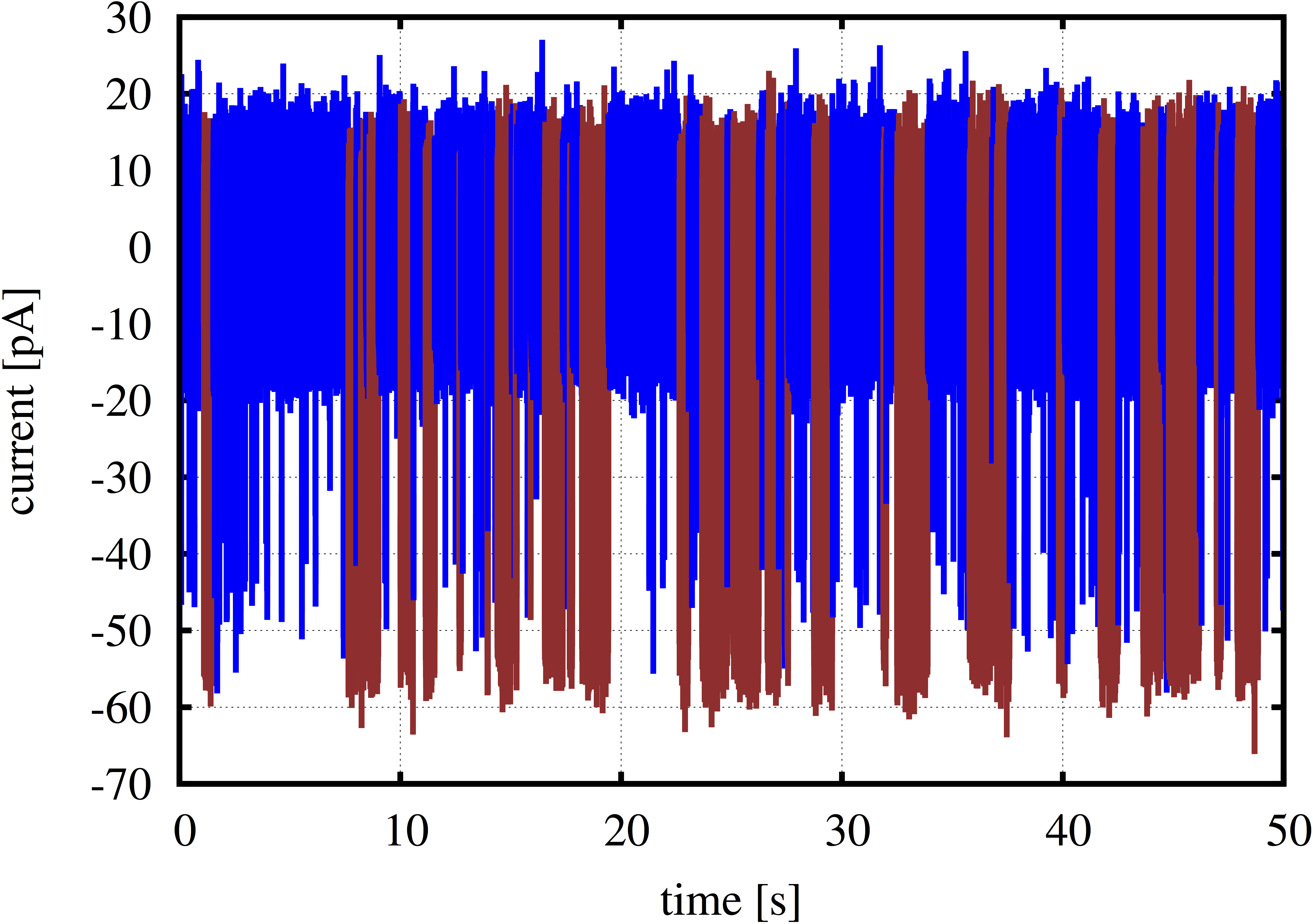
(c) Siekmann et al., 2012b [27] model

Figure 8. The new hierarchical model represents the kinetics more accurately than the model from Siekmann et al., 2012b [27]. Panel (a) shows data from type 2 IP₃R recorded at $10\text{\,}\mu\mathrm{M}$ IP₃, $5\text{\,}\mathrm{m}\mathrm{M}$ ATP and $0.05\text{\,}\mathrm{\SIUnitSymbolMicro}\mathrm{M}$ Ca²⁺. The colour of the line shows in which mode the channel is for a given point in time as inferred by the method of Siekmann et al., [26]. Blue indicates the nearly inactive mode M¹ whereas brown indicates the active mode M². Similar to the data, the time spent in each mode spans a wide range of time scales and the channel alternates between the modes relatively infrequently whereas the model from Siekmann et al., 2012b [27] switches too often.

4. Mathematical analysis of the hierarchical Markov model

In the previous section we demonstrated that the hierarchical Markov model introduced in Section 2 provides a statistically efficient framework for systematically building models for modal gating. Now, we focus on some interesting aspects of the mathematical structure of the hierarchical Markov model and show that many important properties of the infinitesimal generator $M$ of the full model can be derived from the components $\left((\tilde{m}_{0},\tilde{M}),(p^{i},Q^{i})_{i=1}^{n_{M}}\right)$ of the model.

In Section 4.1 we calculate the eigenvalues of $M$. The spectrum of $M$ consists of two parts: the eigenvalues of $\tilde{M}$ and a subset of the eigenvalues of the blocks $M^{i,i}=\tilde{M}^{i,i}\oplus Q^{i}$. But whereas the eigenvalues of the submatrices $\tilde{M}^{i,i}$ appear in the spectrum of the submatrices $M^{i,i}$, they are not eigenvalues of the full model $M$.

From a modelling point of view it is an important question if properties of the components $\left((\tilde{m}_{0},\tilde{M}),(p^{i},Q^{i})_{i=1}^{n_{M}}\right)$ are preserved when they are combined in the full model. In Section 4.2 we demonstrate that the sojourn time distribution in the states representing a particular mode in the model $\tilde{M}$ is preserved for the analogous distribution calculated for the augmented state space of $M$.

When the initial distributions $p^{i}$ coincide with the stationary distributions, $p^{i}=\pi^{i}$, we calculate the full time-dependent solution and the stationary distribution of $M$ from the components $\left((\tilde{m}_{0},\tilde{M}),(p^{i},Q^{i})_{i=1}^{n_{M}}\right)$ of the hierarchical Markov model (Section 4.3).

4.1. Eigenvalues

Before we calculate the eigenvalues for general infinitesimal generators $M$ of the full model we remark that in most cases relevant for ion channel modelling we may assume that the matrices $\tilde{M}$ and $Q^{i}$ appearing in our model are diagonalisable—this is implied by the so-called detailed balance conditions:

(16) $$\pi^{i}q_{ij}=\pi^{j}q_{ji},$$

where $\pi$ is the stationary distribution of an infinitesimal generator $Q=(q_{ij})$. A matrix $Q=(q_{ij})$ with (16) is diagonalisable with real eigenvalues because by choosing the transformation matrix $\operatorname{diag}(\pi)^{1/2}$ it is similar to a symmetric real matrix. Detailed balance is usually assumed to hold for ion channel models because it can be related to thermodynamic reversibility of the transitions between different states in the model. Note that (16) holds automatically if the adjacency graph of the states of a Markov model is acyclic. This follows from Kolmogorov’s criterion [17], see theorem 1.8 of Kelly, [15] for a more recent statement of the continuous-time version. Thus, in particular, all infinitesimal generators $\tilde{M}$ and $Q^{i}$ considered in this article satisfy detailed balance.

Proposition 4.1 (Eigenvalues and eigenvectors of $M$ assuming detailed balance).

We assume that the matrices $\tilde{M}$ and $Q^{i}$ of a hierarchical Markov model fulfil the detailed balance conditions (16).

1. Let $\zeta$ be an eigenvalue of the matrix $\tilde{M}$ and $v_{\boldsymbol{m}}^{T}$ a right eigenvector associated with $\zeta$. Then $\zeta$ is also an eigenvalue of the full model $M$ with associated right eigenvector $v_{\boldsymbol{m}}^{T}\otimes u_{\boldsymbol{n}}^{T}$ where $u_{\boldsymbol{n}}^{T}$ is a vector of $|\boldsymbol{n}|$ ones.

2. Moreover, all $\nu=\tilde{\zeta}+\lambda$, where $\tilde{\zeta}$ is an eigenvalue of $\tilde{M}^{i,i}$ and $\lambda\neq 0$ is an eigenvalue of $Q^{i}$, are eigenvalues of the full model $M$. If $\tilde{w}^{i}$ is a left eigenvector of the submatrix $M^{i,i}$ associated with the eigenvalue $\nu$, $w_{\boldsymbol{m}}=(0;\dots;0;\tilde{w}^{i};0;\dots;0)$ with $w(i)=\tilde{w}^{i}$ and $w(j)=0$, $i\neq j$ is a left eigenvector of $M$ associated with $\nu$.

Proof.

Detailed balance implies that $\tilde{M}$ and the $Q^{i}$ are diagonalisable with real eigenvalues. In particular, all matrices have full sets of eigenvectors. This enables us to construct eigenvectors of the infinitesimal generator $M$ of the full model from the eigenvectors of $\tilde{M}$ and the $Q^{i}$.

1. We need to show that $M(v_{\boldsymbol{m}}^{T}\otimes_{\boldsymbol{m},\boldsymbol{n}}u_{\boldsymbol{n}}^{T})=\zeta(v_{\boldsymbol{m}}^{T}\otimes_{\boldsymbol{m},\boldsymbol{n}}u_{\boldsymbol{n}}^{T})$. Let $[M(v_{\boldsymbol{m}}^{T}\otimes_{\boldsymbol{m},\boldsymbol{n}}u_{\boldsymbol{n}}^{T})]^{i}$ denote the $i$-th component of the partitioned vector. Here, $v_{\boldsymbol{m}}^{T}\otimes_{\boldsymbol{m},\boldsymbol{n}}u_{\boldsymbol{n}}^{T}$ is a tensor product that is consistent with the partitions $\boldsymbol{m}$ and $\boldsymbol{n}$ as in (4) (Definition 2.3). We calculate:

   $$[M(v_{\boldsymbol{m}}^{T}\otimes_{\boldsymbol{m},\boldsymbol{n}}u_{\boldsymbol{n}}^{T})]^{i}=(\tilde{M}^{i,i}\oplus Q^{i})((v^{i})^{T}\otimes u_{n_{i}}^{T})+\sum_{k\neq i}(\tilde{M}^{i,k}\otimes P^{i,k})((v^{k})^{T}\otimes u_{n_{k}}^{T}).$$

   Using the compatibility condition of matrix multiplication and tensor product (27) we calculate:

   $$[M(v_{\boldsymbol{m}}^{T}\otimes_{\boldsymbol{m},\boldsymbol{n}}u_{\boldsymbol{n}}^{T})]^{i} =(\tilde{M}^{i,i}(v^{i})^{T}\otimes u_{n_{i}}^{T}+(v^{i})^{T}\otimes Q^{i}u_{n_{i}}^{T})+\sum_{k\neq i}(\tilde{M}^{i,k}(v^{k})^{T}\otimes P^{i,k}u_{n_{k}}^{T}).$$

   Noting that $Q^{i}u_{n_{i}}^{T}=0$ and $P^{i,k}u_{n_{k}}^{T}=u_{n_{i}}^{T}$ we finally get:

   $$[M(v_{\boldsymbol{m}}^{T}\otimes_{\boldsymbol{m},\boldsymbol{n}}u_{\boldsymbol{n}}^{T})]^{i} =\sum_{k=1}^{n_{M}}\tilde{M}^{i,k}(v^{k})^{T}\otimes u_{n_{i}}^{T}=\zeta((v^{i})^{T}\otimes u_{n_{i}}^{T}).$$

   Because this holds for all blocks we obtain the desired result.

2. All except for the $i$-th block of $w$ are zero, so we get:

   $$wM =(\tilde{w}^{i}[\tilde{M}^{i,1}\otimes P^{1,i}];\dots;\tilde{w}^{i}[\tilde{M}^{i,i}\oplus Q^{i}];\dots;\tilde{w}^{i}[\tilde{M}^{i,n_{M}}\otimes P^{n_{M},i}]).$$

   Because $\tilde{w}^{i}$ is an eigenvector of $\tilde{M}^{i,i}\oplus Q^{i}$ we know that $\tilde{w}^{i}(\tilde{M}^{i,i}\oplus Q^{i})=\nu\tilde{w}^{i}$. For $w$ to be an eigenvector, it remains to be shown that all other blocks vanish. Let $u$ be a left eigenvector of $\tilde{M}^{i,i}$ associated with the eigenvalue $\tilde{\zeta}$ and $v$ a left eigenvector of $Q^{i}$ associated with the eigenvalue $\lambda$. Then $\tilde{w}^{i}$ can be written as $\tilde{w}^{i}=u\otimes v$ according to (28). Substituting this and $P^{i,k}=p^{k}\otimes u_{n_{i}}^{T}$, $k\neq i$, we calculate:

   (17) $$(u\otimes v)[\tilde{M}^{1,k}\otimes p^{k}\otimes u_{n_{i}}^{T}] =u(\tilde{M}^{1,k}\otimes p^{k})\otimes vu_{n_{i}}^{T}.$$

   The term $vu_{n_{i}}^{T}$ is the standard scalar product $\langle v^{T},u_{n_{i}}^{T}\rangle$ of the vectors $v^{T}$ and $u_{n_{i}}^{T}$. Because the row sums of $Q^{i}$ are zero, $u_{n_{i}}^{T}$ is in the right nullspace of $Q^{i}$. By assumption, $v$ is an eigenvector associated to any eigenvalue $\lambda\neq 0$. This means that $v$ is not in the left nullspace of $Q^{i}$, so it must be orthogonal to any vector in the right nullspace. It follows that (17) vanishes as required.

∎

For the general case where the infinitesimal generators of the model $\tilde{M}$ and the submatrices $M^{i,i}$ may not necessarily be diagonalisable we need the Schur decomposition (Proposition A.2). The Schur decomposition ensures that the matrix $M$ can be transformed to an upper-triangular matrix by a unitary matrix. In the following we construct a unitary matrix $S$ from the components $\left((\tilde{m}_{0},\tilde{M}),(p^{i},Q^{i})_{i=1}^{n_{M}}\right)$ of our model.

Lemma 4.1 (Unitary matrix $S$).

For the components $\left((\tilde{m}_{0},\tilde{M}),(p^{i},Q^{i})_{i=1}^{n_{M}}\right)$ of a hierarchical Markov model, let

$$T_{\tilde{M}}=\Theta^{*}\tilde{M}\Theta,\quad T_{\tilde{M}^{i,i}\oplus Q^{i}}=(V_{i}\otimes W_{i})^{*}\tilde{M}^{i,i}\oplus Q^{i}(V_{i}\otimes W_{i}),$$

be the Schur decompositions of $\tilde{M}$ and $\tilde{M}^{i,i}\oplus Q^{i}$. Let $\mathrm{bar}{u}_{n_{i}}^{T}=1/\sqrt{n_{i}}u_{n_{i}}^{T}$ be the vectors obtained by normalising the vectors of ones $u_{n_{i}}^{T}$.

1. The matrices $W_{i}$ may be chosen so that they have the form $W_{i}=\left(\mathrm{bar}{u}_{n_{i}}^{T}\vline\tilde{W}_{i}\right)$ with $\tilde{W}_{i}\in\mathbb{C}^{n_{i}\times(n_{i}-1)}$.

2. Let

   $$\Theta=\begin{pmatrix}\Theta^{1}\\ \hline\cr\vdots\\ \Theta^{n_{M}}\end{pmatrix}$$

   be row-partitioned according to the block structure of $\tilde{M}$ from (1). Then the matrix

   (18) $$S=\begin{pmatrix}\Theta^{1}\otimes\mathrm{bar}{u}_{n_{1}}^{T}&\vline&V_{1}\otimes\tilde{W}_{1}&\vline&0&\vline&\dots&\vline&0\\ \hline\cr\vdots&\vline&0&\vline&V_{2}\otimes\tilde{W}_{2}&\vline&\dots&\vline&\vdots\\ \vdots&&\vdots&&&&\ddots&&0\\ \Theta^{n_{M}}\otimes\mathrm{bar}{u}_{n_{n_{M}}}^{T}&\vline&0&\vline&\dots&\vline&\dots&\vline&V_{n_{M}}\otimes\tilde{W}_{n_{M}}\end{pmatrix}$$

   is unitary.

Proof.

1. Because the row sums of $Q^{i}$ vanish, the vector $\mathrm{bar}{u}_{n_{i}}^{T}$ is a right eigenvector of $Q^{i}$ associated with the eigenvalue zero. Without loss of generality we can choose $\mathrm{bar}{u}_{n_{i}}^{T}$ as the first column of $W_{i}$.

2. By construction, all column vectors of $S$ are normalised. Thus, it remains to show that they are also pairwise orthogonal. By definition, any two distinct column vectors appearing in the same block of $S$ are orthogonal. It is trivial that column vectors from different blocks are orthogonal unless one of the two appears in the first block of $S$. Thus, let $\theta^{T}$ be a column vector of $\Theta$ and $v_{i}^{T}\otimes\tilde{w}_{i}^{T}$ be a column vector of any $V_{i}\otimes W_{i}$. With the shorthand for tensor products consistent with partitions (4) introduced in Definition 2.3, the scalar product $\langle\cdot,\cdot\rangle$ of the two columns is

   $$\langle\theta^{T}_{\boldsymbol{m}}\otimes_{\boldsymbol{m},\boldsymbol{n}}\mathrm{bar}{u}^{T}_{\boldsymbol{n}},(0;\dots;v_{i}\otimes\tilde{w}_{i};\dots 0)^{T}\rangle=\langle\theta^{T}_{\boldsymbol{m}}(i)\otimes\mathrm{bar}{u}^{T}_{n_{i}},v_{i}^{T}\otimes\tilde{w}_{i}^{T}\rangle$$

   and due to the zeroes in all except for the $i$-th block, all other summands vanish. Noting that $\langle u,v\rangle=u(v^{*})^{T}=u^{T}v^{*}$ can be interpreted as a special case of matrix multiplication (where ‘$*$’ denotes component-wise complex conjugation) we can use (27):

   $$\langle\theta^{T}_{\boldsymbol{m}}(i)\otimes_{\boldsymbol{m},\boldsymbol{n}}\mathrm{bar}{u}^{T}_{n_{i}},v_{i}^{T}\otimes\tilde{w}_{i}^{T}\rangle=\langle\theta^{T}_{\boldsymbol{m}}(i),v^{T}_{i}\rangle\langle\mathrm{bar}{u}^{T}_{n_{i}},\tilde{w}_{i}^{T}\rangle.$$

   But because $\mathrm{bar}{u}^{T}_{n_{i}}$ appeared as a column in the original unitary matrix $W_{i}$, the $\tilde{w}_{i}^{T}$ are all orthogonal to $\mathrm{bar}{u}^{T}_{n_{i}}$ so that the above scalar product vanishes. Thus, the matrix $S$ is unitary.

∎

Proposition 4.2 (Eigenvalues of the full model $M$).

Let $\tilde{\zeta}$ be an eigenvalue of the model $\tilde{M}$. Then $\tilde{\zeta}$ is also an eigenvalue of the full model $M$. Moreover, all $\nu=\tilde{\zeta}+\lambda$, where $\tilde{\zeta}$ is an eigenvalue of $\tilde{M}^{i,i}$ and $\lambda\neq 0$ is an eigenvalue of $Q^{i}$, are eigenvalues of the full model $M$.

Proof.

We demonstrate that with the matrix $S$ from (18) we obtain a Schur decomposition of the matrix $M$. We need to show that $A=S^{*}MS$ is upper triangular. The block structure of $S$ is rectangular with $n_{M}\times(n_{M}+1)$ blocks which means that $S^{*}$ has an $(n_{M}+1)\times n_{M}$ block structure. Thus, the resulting matrix $A$ will have $(n_{M}+1)\times(n_{M}+1)$ blocks and its diagonal will consist of the eigenvalues of $\tilde{M}$ in the upper left block followed by the remaining eigenvalues from the submatrices $\tilde{M}^{i,i}$. We show that all blocks $A^{i,j}$ are upper triangular which implies that $A$ is indeed upper triangular. First, a lengthy calculation shows that $A^{1,1}$ is a block-wise expanded form of $\Theta^{*}\tilde{M}\Theta$ and thus upper-triangular. One can see directly that the remaining elements on the block diagonal are

$$A^{i,i}=(V_{i}\otimes\tilde{W}_{i})^{*}(\tilde{M}^{i,i}\oplus Q^{i})(V_{i}\otimes\tilde{W}_{i})$$

and therefore all upper triangular.

It remains to show that the lower diagonal blocks $A^{i,j}$ with $i>j$ vanish. We will demonstrate that the $A^{i,j}$ vanish provided that

(19) $$\tilde{W}_{i}^{*}\mathrm{bar}{u}^{T}_{n_{i}}=0.$$

Equation (19) is just another way of saying that $\mathrm{bar}{u}_{n_{i}}^{T}$ is orthogonal to all columns of $\tilde{W}_{i}$. But this is true because from Lemma 4.1(i) we know that $\mathrm{bar}{u}_{n_{i}}^{T}$ is the first column of $W_{i}$, so it must be orthogonal to all column vectors of $\tilde{W}_{i}$.

We now calculate the subdiagonal blocks $A^{i,j}$, $i>j$. First we calculate the blocks $A^{\cdot,1}$ on the first block column. We observe that

$$(M\cdot S)^{k,1}=(\tilde{M}^{k,k}\oplus Q^{k})(\Theta^{k}\otimes\mathrm{bar}{u}_{n_{k}}^{T})+\sum_{j\neq k}(\tilde{M}^{k,j}\otimes P^{k,j})(\Theta^{j}\otimes\mathrm{bar}{u}_{n_{j}}^{T}).$$

Because $S^{*}$ is block-diagonal below the first row we can calculate

$$A^{k+1,1}=(S^{*}\cdot M\cdot S)^{k+1,1} =(V_{k}\otimes\tilde{W}_{k})^{*}(\tilde{M}^{k,k}\oplus Q^{k})(\Theta^{k}\otimes\mathrm{bar}{u}_{n_{k}}^{T})$$

$$+\sum_{j\neq k}(V_{k}\otimes\tilde{W}_{k})^{*}(\tilde{M}^{k,j}\otimes P^{k,j})(\Theta^{j}\otimes\mathrm{bar}{u}_{n_{j}}^{T})$$

because in the row $(k+1)$-th row of $S^{*}$ for $k=1,\dots,n_{M}$ only the $k$-th block is non-zero. By taking advantage of (27) we obtain

$$A^{k+1,1} =(V_{k}\otimes\tilde{W}_{k})^{*}(\tilde{M}^{k,k}\Theta^{k}\otimes\mathrm{bar}{u}_{n_{k}}^{T}+\Theta^{k}\otimes Q^{k}\mathrm{bar}{u}_{n_{k}}^{T})$$

$$+\sum_{j\neq k}(V_{k}\otimes\tilde{W}_{k})^{*}(\tilde{M}^{k,j}\Theta^{j}\otimes P^{k,j}\mathrm{bar}{u}_{n_{j}}^{T})$$

$$=(V_{k}\otimes\tilde{W}_{k})^{*}(\tilde{M}^{k,k}\Theta^{k}\otimes\mathrm{bar}{u}_{n_{k}}^{T})$$

$$+\sum_{j\neq k}(V_{k}\otimes\tilde{W}_{k})^{*}(\tilde{M}^{k,j}\Theta^{j}\otimes\mathrm{bar}{u}_{n_{k}}^{T})$$

where we have used $Q^{k}\mathrm{bar}{u}_{n_{k}}^{T}=0$ and $P^{k,j}\mathrm{bar}{u}_{n_{j}}^{T}=\mathrm{bar}{u}_{n_{k}}^{T}$. Again using (27) we calculate

$$A^{k+1,1} =V_{k}^{*}\tilde{M}^{k,k}\Theta^{k}\otimes\tilde{W}_{k}^{*}\mathrm{bar}{u}_{n_{k}}^{T})$$

$$+\sum_{j\neq k}V_{k}^{*}\tilde{M}^{k,j}\Theta^{j}\otimes\tilde{W}_{k}^{*}\mathrm{bar}{u}_{n_{k}}^{T})$$

This vanishes due to (19) as explained above.

For the remaining blocks $A^{k+1,l+1}$, $k>l=1,\dots,n_{M}-1$ we simply calculate

$$A^{k+1,l+1} =(V_{k}\otimes\tilde{W}_{k})^{*}(\tilde{M}^{k,l}\otimes P^{k,l})(V_{l}\otimes\tilde{W}_{l})$$

$$=(V_{k}^{*}\tilde{M}^{k,l}\otimes\tilde{W}_{k}^{*}P^{k,l})(V_{l}\otimes\tilde{W}_{l})$$

$$=(V_{k}^{*}\tilde{M}^{k,l}V_{l})\otimes(\tilde{W}_{k}^{*}P^{k,l}\tilde{W}_{l}).$$

Replacing $P^{k,l}$ by $\mathrm{bar}{u}_{n_{k}}^{T}\otimes p^{l}$ (6) we get

$$A^{k+1,l+1}=(V_{k}^{*}\tilde{M}^{k,l}V_{l})\otimes(\tilde{W}_{k}^{*}\mathrm{bar}{u}_{n_{k}}^{T})\otimes(p^{l}\tilde{W}_{l})$$

where—due to the term $\tilde{W}_{k}^{*}\mathrm{bar}{u}_{n_{k}}^{T}$—we again conclude with (19) that $A^{k+1,l+1}$ vanishes.

∎

4.2. Sojourn times in modes

We will now investigate the sojourn times within the states that represent the modes $\text{M}^{i}$. The switching between modes is represented by a model with infinitesimal generator $\tilde{M}$ and one can ask if the dynamics is preserved after $\tilde{M}$ is combined with the other components $\left((\tilde{m}_{0},\tilde{M}),(p^{i},Q^{i})_{i=1}^{n_{M}}\right)$ to the generator $M$ of the full model . We denote by $f_{\tilde{M}^{i}}(t)$ the density function of the sojourn time in mode $\text{M}^{i}$ represented by $\tilde{M}$ and by $f_{\text{M}^{i}}(t)$ the sojourn time densities of $\text{M}^{i}$ in the augmented state space of the generator $M$ of the full model. If the mode switching dynamics is preserved, the sojourn time densities should be equal and we will show that indeed $f_{\text{M}^{i}}(t)=f_{\tilde{M}^{i}}(t)$.

Proposition 4.3 (Modal sojourn times).

For $f_{\text{M}^{i}}(t)$, sojourn time densities within mode $\text{M}^{i}$ with an initial distribution $p^{0}$ as in Definition 8, we have $f_{\text{M}^{i}}(t)=f_{\tilde{M}^{i}}(t)$.

Proof.

For simplicity we only treat the case of two aggregates of states, $M^{1}$ and $M^{2}$. For the sojourn time within $M^{1}$ we have

$$f_{M^{1}}(t)=p^{0}M^{2,1}\exp\left(M^{1,1}t\right)M^{1,2}u_{m_{2}n_{2}}^{T}$$

where $p^{0}=p_{\tilde{M}^{2}}^{0}\otimes p_{Q^{2}}^{0}$ is a suitably normalised initial state probability distribution. Substituting from (7) we obtain for

$$\exp\left(M^{1,1}t\right)M^{1,2} =\exp\left(\left[\tilde{M}^{1,1}\oplus Q^{1}\right]t\right)M^{1,2}$$

$$=\left[\exp\left(\tilde{M}^{1,1}t\right)\otimes\exp\left(Q^{1}t\right)\right]\left(\tilde{M}^{1,2}\otimes P^{1,2}\right)$$

where we have used (29) for calculating the matrix exponential. Now,

$$\left[\exp\left(\tilde{M}^{1,1}t\right)\otimes\exp\left(Q^{1}t\right)\right]\left(\tilde{M}^{1,2}\otimes P^{1,2}\right) =\left[\exp\left(\tilde{M}^{1,1}t\right)\tilde{M}^{1,2}\right]\otimes P^{1,2}$$

according to the compatibility of tensor and matrix product (27) which will be used repeatedly below. Also note that $\exp\left(Q^{1}t\right)\cdot P^{1,2}=P^{1,2}$. Multiplying this on the right by $u_{m_{2}n_{2}}^{T}=u_{m_{2}}^{T}\otimes u_{n_{2}}^{T}$ leads to

$$\left\{\left[\exp\left(\tilde{M}^{1,1}t\right)\tilde{M}^{1,2}\right]\otimes P^{1,2}\right\}\left(u_{m_{2}}^{T}\otimes u_{n_{2}}^{T}\right)=\left[\exp\left(\tilde{M}^{1,1}t\right)\tilde{M}^{1,2}u_{m_{2}}^{T}\right]\otimes u_{n_{1}}^{T}$$

where we have evaluated $P^{1,2}u^{T}_{n_{2}}=u^{T}_{n_{1}}$ in the right-most term. Analogous calculations will be carried out automatically below. The above result is now multiplied on the left by $M^{2,1}=\tilde{M}^{2,1}\otimes P^{2,1}$:

$$\left(\tilde{M}^{2,1}\otimes P^{2,1}\right)\left[\exp\left(\tilde{M}^{1,1}t\right)\tilde{M}^{1,2}u_{m_{2}}^{T}\right]\otimes u_{n_{1}}^{T}=\left[\tilde{M}^{2,1}\exp\left(\tilde{M}^{1,1}t\right)\tilde{M}^{1,2}u_{m_{2}}\right]\otimes u_{n_{2}}^{T}.$$

Finally we multiply the preceding result on the left by $p^{0}=p_{\tilde{M}^{2}}^{0}\otimes p_{Q^{2}}^{0}$ and compute

$$f_{M^{1}}(t) =\left(p_{\tilde{M}^{2}}^{0}\otimes p_{Q^{2}}^{0}\right)\left[\tilde{M}^{2,1}\exp\left(\tilde{M}^{1,1}t\right)\tilde{M}^{1,2}u_{m_{2}}\right]\otimes u_{n_{2}}^{T}$$

$$=\left[p_{\tilde{M}^{2}}^{0}\tilde{M}^{2,1}\exp\left(\tilde{M}^{1,1}t\right)\tilde{M}^{1,2}u_{m_{2}}^{T}\right]\otimes\left(p_{Q^{2}}^{0}u_{n_{2}}^{T}\right).$$

Now, because $\left(p_{Q^{2}}^{0}u_{n_{2}}^{T}\right)=1$ we obtain the desired result:

$$f_{M^{1}}(t) =p_{\tilde{M}^{2}}^{0}\tilde{M}^{2,1}\exp\left(\tilde{M}^{1,1}t\right)\tilde{M}^{1,2}u_{m_{2}}^{T}=f_{\tilde{M}^{1}}(t).$$

∎

4.3. Full solution for $p^{i}=\pi^{i}$

If we choose initial conditions $p^{i}=\pi^{i}$, where the $\pi^{i}$ are stationary distributions of the models $Q^{i}$, the solution of the full model has a particularly simple form.

Proposition 4.4 (Full solution for $p^{i}=\pi^{i}$).

Let $v_{\boldsymbol{m}}(t)$ be the time-dependent solution for the initial condition $w_{\boldsymbol{n}}^{0}$ and $\tilde{\mu}_{\boldsymbol{n}}$ be the stationary solution of the infinitesimal generator $\tilde{M}$ with their partition ${\boldsymbol{m}}$. Let $\pi^{i}$, $i=1,\dots,n_{M}$ be the stationary distributions of $Q^{i}$ or written as a partitioned vector, $\pi_{\boldsymbol{n}}$ with its partition ${\boldsymbol{n}}$. If for each generator $Q^{i}$ we set $p^{i}=\pi^{i}$ and we choose an initial distribution $p^{0}_{\boldsymbol{m}\cdot\boldsymbol{n}}=v_{\boldsymbol{m}}^{0}\otimes_{\boldsymbol{m},\boldsymbol{n}}\pi_{\boldsymbol{n}}$ consistent with Definition 8, the solution $p_{{\boldsymbol{m}}\cdot{\boldsymbol{n}}}(t)$ of the full model is

(20) $$p_{{\boldsymbol{m}}\cdot{\boldsymbol{n}}}(t)=v_{\boldsymbol{m}}(t)\otimes_{\boldsymbol{m},\boldsymbol{n}}\pi_{\boldsymbol{n}}=(v^{1}(t)\otimes\pi^{1};\dots;v^{i}(t)\otimes\pi^{i};\dots;v^{n_{M}}\otimes\pi^{n_{M}}).$$

By taking the limit $t\to\infty$ we obtain the stationary distribution

(21) $$\mu_{{\boldsymbol{m}}\cdot{\boldsymbol{n}}}=\tilde{\mu}_{\boldsymbol{m}}\otimes_{\boldsymbol{m},\boldsymbol{n}}\pi_{\boldsymbol{n}}=(\tilde{\mu}^{1}\otimes\pi^{1};\dots;\tilde{\mu}^{i}\otimes\pi^{i};\dots;\tilde{\mu}^{n_{M}}\otimes\pi^{n_{M}}).$$

Remark 4.1.

The stationary distribution (21) is independent of the initial distribution $p^{0}_{\boldsymbol{m}\cdot\boldsymbol{n}}$, so, for $p^{i}=\pi^{i}$, we converge to the stationary distribution (21) also for $p^{0}_{\boldsymbol{m}\cdot\boldsymbol{n}}=(v_{\boldsymbol{m}}^{0}\otimes_{\boldsymbol{m},\boldsymbol{n}}w_{\boldsymbol{n}}^{0})$ with $w_{\boldsymbol{n}}^{0}\neq\pi_{\boldsymbol{n}}$ and even for arbitrary initial conditions $p^{0}_{\boldsymbol{m}\cdot\boldsymbol{n}}$ that are inconsistent with Definition 8.

Proof.

That (20) is a solution can be shown by substituting $p_{\boldsymbol{m}\cdot\boldsymbol{n}}(t)=v_{\boldsymbol{m}}(t)\otimes_{\boldsymbol{m},\boldsymbol{n}}\pi_{\boldsymbol{n}}$ into

(22) $$\frac{dp(t)}{dt}=p(t)M,$$

where $M$ is the generator of the full model (7). First we calculate the left-hand side:

$$\frac{dp_{\boldsymbol{m}\cdot\boldsymbol{n}}(t)}{dt} =\frac{d\left(v_{\boldsymbol{m}}(t)\otimes_{\boldsymbol{m},\boldsymbol{n}}\pi_{\boldsymbol{n}}\right)}{dt}$$

$$=\left(\frac{dv_{\boldsymbol{m}}(t)}{dt}\right)\otimes_{\boldsymbol{m},\boldsymbol{n}}\pi_{\boldsymbol{n}}$$

(23) $$=\left(v_{\boldsymbol{m}}(t)\tilde{M}\right)\otimes_{\boldsymbol{m},\boldsymbol{n}}\pi_{\boldsymbol{n}}$$

where the last equality (23) follows because $v_{\boldsymbol{m}}(t)$ is a solution of the model generated by $\tilde{M}$.

We now show that we also obtain (23) from the right-hand side of (22). For the $i$-th component $[p_{\boldsymbol{m}\cdot\boldsymbol{n}}(t)\cdot M]^{i}$ we calculate

$$[p_{\boldsymbol{m}\cdot\boldsymbol{n}}(t)\cdot M]^{i} =\left(v^{i}(t)\otimes\pi^{i}\right)\left(\tilde{M}^{i,i}\oplus Q^{i}\right)+\sum_{j\neq i}\left(v^{j}(t)\otimes\pi^{j}\right)\left(\tilde{M}^{j,i}\otimes P^{j,i}\right)$$

For the first summand the contribution of $Q^{i}$ vanishes because of $\pi^{i}Q^{i}=0$

(24) $$\left(v^{i}(t)\otimes\pi^{i}\right)\left(\tilde{M}^{i,i}\oplus Q^{i}\right)=\left(v^{i}(t)\tilde{M}^{i,i}\right)\otimes\pi^{i}+v^{i}(t)\otimes\pi^{i}Q^{i}=\left(v^{i}(t)\tilde{M}^{i,i}\right)\otimes\pi^{i}.$$

Because of $\pi^{j}P^{j,i}=\pi^{i}$ the second summand simplifies to

(25) $$\sum_{j\neq i}\left(v^{j}(t)\otimes\pi^{j}\right)\left(\tilde{M}^{j,i}\otimes P^{j,i}\right)=\sum_{j\neq i}\left(v^{j}(t)\tilde{M}^{j,i}\right)\otimes\pi^{i}.$$

With (24) and (25) we derive for each component:

$$[p_{\boldsymbol{m}\cdot\boldsymbol{n}}(t)\cdot M]^{i}=\sum_{i=1}^{n_{M}}\left(v^{j}(t)\tilde{M}^{j,i}\right)\otimes\pi^{i}.$$

This means that the right-hand side of (22) is indeed of the form (23) which confirms that (20) is a solution.

∎

5. Conclusion

We have proposed a new model for representing modal gating, the spontaneous switching of ion channels between different levels of activity. The model is suitable for modelling channels with an arbitrary number of modes and is capable of representing both the probabilistic opening and closing within modes as well as the stochastic switching between modes that regulates these dynamics.

5.1. Modular representation of modal gating

In comparison with previous studies, the model presented here incorporates modal gating in a much more transparent way. Ullah et al., [29] developed their model of the IP₃R from a binding scheme. First, the authors determined the set of open and closed model states from a statistical model selection criterion. Second, they determined which of these states should account for which of the three modes observed by Ionescu et al., [14]. The decision that a particular open or closed state should account for the mode showing a low, intermediate or high level of activity was based on heuristic inspection of the ligand-dependency of modal gating. The model was parameterised by optimising a likelihood that accounted for various sources of single channel data including statistics of modal gating. This treats the parameter space of their model as a black box from which a suitable set of parameters capable of accounting for all data sets is selected by optimisation. We expect such an approach to be statistically less efficient than a model whose structure incorporates modal gating more explicitly.

Siekmann et al., 2012b [27] used modal gating as the underlying construction principle of their model by separating the inference of parameters related to dynamics within modes from estimation of parameters related to switching between modes. First, models for the inactive mode M¹ and the active mode M² were inferred by fitting segments of data representative of each of the two modes—in fact, the same models were re-used in the present study. However, because at that time rigorous statistical techniques for segmenting ion channel data by modes were not available, the time scales of the switching between both modes was inferred by connecting the submodels for M¹ and M² with a pair of transition rates whose values were then determined from a fit to complete traces of single channel data. Similar to Ullah et al., [29] modal gating was thus incorporated into the model without explicitly considering its stochastic dynamics apparent in the data.

The model presented here improves the model from Siekmann et al., 2012b [27] by explicitly modelling modal gating. After the stochastic process of switching between modes has been extracted from the data using a statistical method such as Siekmann et al., [26] instead of arbitrarily introducing transition rates between modes as in our previous study, we instead fit a model $\tilde{M}$ directly to the stochastic process of mode switching. This enables us to accurately represent mode switching, only adding exactly as many parameters as required. In comparison to our previous model, the new model described here requires only two additional parameters. Inspection of the sojourn time histograms show that these two parameters are essential in order to account for the fact that sojourns in the nearly inactive mode M¹ exhibit two different time scales which cannot be represented by a model with less parameters.

It is important to note that none of the components $\left((\tilde{m}_{0},\tilde{M}),(p^{i},Q^{i})_{i=1}^{n_{M}}\right)$ of our model are determined by fitting to the sequence of open and closed events observed in experiments—the models $Q^{i}$ are inferred from segments of the data and the model $\tilde{M}$ is parametrised from transitions between the modes $\text{M}^{i}$. Thus, the open and closed time distributions $f_{O}(t)$ and $f_{C}(t)$, respectively, can be considered a prediction of our hierarchical model $M$. That the hierarchical model $M$ outperforms our previous model whose transition rates were inferred from a direct fit to complete traces of open and closed events indicates that the new approach is a superior representation of the data.

The modular structure of our hierarchical model which separates the representation of transitions between modes (inter-modal kinetics) from the dynamics within modes (intra-modal kinetics) not only provides a more parsimonious representation than previous models but, most notably, evidence is accumulating that mode switching is more important for ion channel function than intra-modal kinetics. This was recently shown in two studies of the role of IP₃R in intracellular calcium dynamics. Cao et al., [2] showed that the essential features of calcium oscillations in airway smooth muscle could be preserved after iteratively simplifying the model from Siekmann et al., 2012b [27] to a two-state model that only accounted for switching between the two modes neglecting the kinetics of transitions between multiple open and closed states within the modes. Siekmann et al., [24] applied similar reduction techniques to demonstrate that also the stochastic dynamics of small clusters of IP₃Rs can be captured by a two-state model reduced to the dynamics of mode switching. In our new hierarchical model, inter-modal and intra-modal kinetics are represented separately so that the model representation with the right level of detail can be chosen based on the requirements of a specific application.

5.2. Biophysical implications of modal gating

Although modal gating has been observed for a long time it has rarely been accounted for in ion channel models. The crucial importance of modal gating has only recently been appreciated among investigators of the IP₃R channel and it is now widely recognised in the community [20]. Various independent sources of evidence indicate that modal gating must be accounted for, both for understanding IP₃R function as well as for gaining insight into biophysical properties of the channel molecule. As mentioned in the previous section, the role of IP₃R in intracellular calcium dynamics is defined by its behaviour on the slow time scale of transitions between different modes rather than the fast time scale of opening and closing [2, 24]. Previously, Ionescu et al., [14] discovered that the IP₃R adjusts its level of activity depending on ligands such as calcium by regulating the proportion of time that the channel spends in different modes. This was subsequently confirmed by the statistical analysis by Siekmann et al., [26]. Whereas these results reveal the major functional implications of modal gating, a detailed analysis of the potassium channel KscA, discussed in more detail below, gives insight into how different modes arise from biophysical constraints of the channel protein [5, 4, 3]. More recently, Vij et al., [30] published a similar study in acetylcholine receptors. Also see the commentary by Geng and Magleby, [11]. This suggests that modes form a fixed repertoire of possible behaviours defined by the molecular properties of the channel. Being constrained to a few different modes, ion channels overcome these limitations by switching between modes.

This interpretation implies that appropriate analysis of modal gating may enable us to extract information on the transitions between different biophysical states from single channel data which—apart from giving an accurate representation of its dynamics—has always been a strong motivation for modelling ion channels. The simplest possible representation of an ion channel is a two-state Markov model with only one open and one closed state. Because opening of the channel involves a rearrangement of the three-dimensional structure of the channel protein, known as a conformational change, it is clear that these two different model states at the same time correspond to different biophysical states of the channel protein. Thus, the transition rates between the open and the closed state provide not just a descriptive representation of the time scale of opening and closing but, in fact, may stand for the dynamics of a biophysical process, the conformational change involved with the opening of the channel. This “mechanistic” interpretation explains the popularity of this type of model. On the one hand the Markov assumption implies that open and closed times are exponentially distributed which means that durations of channel openings and closings both have characteristic time scales $\tau_{O}$ and $\tau_{C}$ given by the parameters of the exponential sojourn time distributions $f_{O}(t)$ and $f_{C}(t)$. However, many ion channels exhibit multiple characteristic open and closed times that cannot be represented by exponential distributions. On the other hand whereas an open ion channel must be in a different conformation than a closed ion channel distinguishing only two conformational states is a very coarse description of the complicated deformations of channel proteins that can be identified by molecular dynamics models. Nevertheless, if our goal is to base our models on rigorous statistical analysis, for some data we may not be able to identify more than two states.

Non-exponential open and closed times can often be represented satisfactorily by aggregated continuous-time Markov models where more than one state is used for representing the channel being open or closed. These models provide a simple generalisation of the two-state Markov model and account for more than just one characteristic open or closed time scale $\tau_{O}$ and $\tau_{C}$. By definition, the sojourn times in the open or closed class of an aggregated Markov model are distributed according to a phase-type distribution, a class of distributions representing the time a Markov chain spends in a set of transient states until exiting to an absorbing state [22, 23]. As with the two-state model it is tempting to also associate the individual states of an aggregated Markov model with different biophysical states of the channel protein. The multiple open and closed states of an aggregated Markov model could be interpreted to resolve in more detail the series of conformational changes that the channel goes through while it opens. If this interpretation was valid one could hope to discover details of the molecular structure of ion channels beyond the trivial distinction between an open and a closed state once the “best” aggregated Markov model for a given data set has been found.

Unfortunately, this “mechanistic” interpretation of aggregated Markov models has several flaws. First, the only reason that a particular model consists of multiple open and closed states is that multiple characteristic open and closed times were observed. Identifying each of these states with a distinct conformational state relies mostly on the analogy with the two-state model with at best little and usually no empirical evidence. Neither experimental techniques nor biophysical modelling approaches currently available enable us to identify a three-dimensional configuration of the channel protein that corresponds to a model state with a short open time and distinguish it from another conformational state that is characterised by a long open time. If we allow the time scale of conformational changes to be non-exponentially distributed in general, multiple open or closed states may actually be associated with the same conformation. In contrast, it is likely that some conformational states may not have a strong enough influence on the dynamics that they are represented by a state in a model inferred from the data. Second, and more importantly, aggregated Markov models are only defined up to equivalence [9, 10, 16, 1, 25] with other models having the same number of open and closed states. In particular, it can be shown that models with completely different adjacency matrices can describe the same process [16] although there is a canonical phase-type description, given, for example, by its Laplace-Stieltjes transform. Thus, interpreting the graphical structure of an aggregated Markov model as a description of possible transitions between different conformational states is not necessarily meaningful without further data. A related problem is the fact that some adjacency matrices lead to non-identifiable models, in particular, certain types of cyclic models are non-identifiable. Whereas it is unlikely that transitions between conformational states underlie any fundamental restrictions of this kind, only some of these transitions would be identifiable from experimental data. It is important to note that the described challenge of relating aggregated Markov models with biophysical processes does not restrict in any way their capability of statistically capturing the stochastic dynamics of ion channels. This only demonstrates that aggregated Markov models are a more abstract representation than they may appear to be at first glance.

In contrast, interpreting mode switching as transitions between distinct biophysical states does not suffer from these difficulties. Chakrapani et al., 2007b [5], Chakrapani et al., 2007a [4], Chakrapani et al., [3] were able to restrict the KscA channel to one of its normally four modes by mutating a particular site of the amino acid sequence of the channel protein. Combining crystallography imaging and molecular dynamics modelling they could further demonstrate that the four modes were related to different conformational states of the channel. It is therefore likely that switching between distinct characteristic dynamical patterns in single channel data can be directly associated with the transition from one to another conformation of the channel protein. This implies that models which accurately represent mode switching can also be used to infer the time scales of transitions between biophysical states associated with these modes. This opens up the exciting possibility that we can gain insight into biophysical processes involved in ion channel gating by statistical analysis and modelling of single channel data rather than having to rely on more time-consuming experimental techniques such as crystallography or more laborious modelling techniques such as molecular dynamics.

Funding

This research was in part conducted and funded by the Australian Research Council Centre of Excellence in Convergent Bio-Nano Science and Technology (project number CE140100036). P. Taylor is supported by the Australian Research Council (ARC) Laureate Fellowship FL130100039 and the ARC Centre of Excellence for Mathematical and Statistical Frontiers (ACEMS).

Appendix A Mathematical background

The results presented in the main text are derived from the following properties of the Kronecker product and sum and some well-known results from linear algebra.

Proposition A.1 (Properties of Kronecker product $\otimes$ and Kronecker sum $\oplus$).

The following properties of the Kronecker product and sums can all be found in Horn and Johnson, [13].

1. Transposition and conjugate transpose (Properties 4.2.4 and 4.2.5):

   (26) $$(A\otimes B)^{T}=A^{T}\otimes B^{T},\quad(A\otimes B)^{*}=A^{*}\otimes B^{*}.$$

2. Compatibility of tensor product and matrix multiplication (Lemma 4.2.10): Let $A\in\mathbb{R}^{k_{1}\times m_{1}}$, $C\in\mathbb{R}^{m_{1}\times n_{1}}$, $B\in\mathbb{R}^{k_{2}\times m_{2}}$, $D\in\mathbb{R}^{m_{2}\times n_{2}}$.

   (27) $$(A\otimes B)(C\otimes D)=(AC)\otimes(BD)\in\mathbb{R}^{k_{1}k_{2}\times n_{1}n_{2}}.$$

3. Eigenvalues of Kronecker sums $A\oplus B$ (Theorem 4.4.5): Let $\alpha$, $\beta$ denote eigenvalues of the square matrices $A$ and $B$. Then the eigenvalues of $M=A\oplus B$ are

   (28) $$\gamma=\alpha+\beta.$$

4. Matrix exponentials of Kronecker sums (Chapter 6, Problem 14): For square matrices $A\in\mathbb{R}^{m\times m}$ and $B\in\mathbb{R}^{n\times n}$:

   (29) $$\exp\left(A\oplus B\right)=\exp(A)\otimes\exp(B)\in\mathbb{R}^{mn\times mn}.$$

If we cannot assume that a matrix has a complete set of eigenvectors so that it may not be diagonalisable we can still triangularise this matrix over the complex numbers $\mathbb{C}$. The process of triangulation can be described by the Schur decomposition:

Proposition A.2 (Schur decomposition).

For a square matrix $A\in\mathbb{R}^{m\times m}$ there exists a unitary matrix $\Theta\in\mathbb{C}^{m\times m}$ and an upper triangular matrix $T$ such that

(30) $$T=\Theta^{*}A\Theta$$

where $\Theta^{*}$ is the conjugate transpose of $\Theta$; (30) is known as the Schur decomposition.
Let $A\in\mathbb{R}^{m\times m}$ and $B\in\mathbb{R}^{n\times n}$ with Schur decompositions

$$T_{A}=V^{*}AV,\quad T_{B}=W^{*}BW.$$

Schur decompositions for the Kronecker product $A\otimes B$ and the Kronecker sum $A\oplus B$ can then be obtained via

(31) $$T_{A\otimes B}=(V\otimes W)^{*}A\otimes B(V\otimes W),\quad T_{A\oplus B}=(V\otimes W)^{*}A\oplus B(V\otimes W).$$

Proof.

See Horn and Johnson, [12], theorem 2.3.1. For (31) we refer to the proofs of Theorems 4.2.12 and 4.4.5 in Horn and Johnson, [13]. ∎

References

- Bruno et al., [2005] Bruno, W. J., Yang, J., and Pearson, J. E. (2005). Using independent open-to-closed transitions to simplify aggregated Markov models for ion channel gating kinetics. Proceedings of the National Academy of Science of the United States of America, 102(16): 6326–6331.
- Cao et al., [2014] Cao, P., Tan, X., Donovan, G., Sanderson, M. J., and Sneyd, J. (2014). A deterministic model predicts the properties of stochastic calcium oscillations in airway smooth muscle cells. PLoS Computational Biology, 10(8): e1003783.
- Chakrapani et al., [2011] Chakrapani, S., Cordero-Morales, J. F., Jogini, V., Pan, A. C., Cortes, D. M., Roux, B., and Perozo, E. (2011). On the structural basis of modal gating behaviour in K+ channels. Nature Structural and Molecular Biology, 18(1): 67–75.
- [4] Chakrapani, S., Cordero-Morales, J. F., and Peroso, E. (2007a). A quantitative description of KscA gating II: Single-channel currents. Journal of General Physiology, 130(5): 479–496.
- [5] Chakrapani, S., Cordero-Morales, J. F., and Perozo, E. (2007b). A quantitative description of KscA gating I: Macroscopic currents. Journal of General Physiology, 130(5): 465–478.
- Christen and Fox, [2010] Christen, J. A. and Fox, C. (2010). A general purpose sampling algorithm for continuous distributions (the t-walk). Bayesian Analysis, 5(2): 263–282.
- Colquhoun and Hawkes, [1981] Colquhoun, D. and Hawkes, A. G. (1981). On the stochastic properties of single ion channels. Proceedings of the Royal Society of London B, 211: 205–235.
- Fine et al., [1998] Fine, S., Singer, Y., and Tishby, N. (1998). The hierarchical hidden Markov model: Analysis and applications. Machine Learning, 32: 41–62.
- Fredkin et al., [1985] Fredkin, D. R., Montal, M., and Rice, J. A. (1985). Identification of aggregated Markovian models: Application to the nicotinic acetylcholine receptor. In L. M. L. Cam and R. A. Olshen (Eds.), Proceedings of the Berkeley Conference in Honor of Jerzy Neyman and Jack Kiefer, volume 1 (pp. 269–289). Belmont, CA: Wadsworth.
- Fredkin and Rice, [1986] Fredkin, D. R. and Rice, J. A. (1986). On aggregated Markov processes. Journal of Applied Probability, 23(1): 208–214.
- Geng and Magleby, [2015] Geng, Y. and Magleby, K. L. (2015). Modal gating of endplate acetylcholine receptors: A proposed mechanism. The Journal of General Physiology, 146(6): 435–439.
- Horn and Johnson, [1985] Horn, R. A. and Johnson, C. R. (1985). Matrix Analysis. Cambridge University Press. Cambridge Books Online.
- Horn and Johnson, [1994] Horn, R. A. and Johnson, C. R. (1994). Topics in Matrix Analysis. Cambridge ; New York : Cambridge University Press, 1994.
- Ionescu et al., [2007] Ionescu, L., White, C., Cheung, K.-H., Shuai, J., Parker, I., Pearson, J. E., Foskett, J. K., and Mak, D.-O. D. (2007). Mode switching is the major mechanism of ligand regulation of InsP3 receptor calcium release channels. Journal of General Physiology, 130(6): 631–645.
- Kelly, [2011] Kelly, F. P. (2011). Reversibility and Stochastic Networks. Cambridge University Press, 2nd edition.
- Kienker, [1989] Kienker, P. (1989). Equivalence of aggregated Markov models of ion-channel gating. Proceedings of the Royal Society of London B, 236: 269–309.
- Kolmogorov, [1936] Kolmogorov, A. N. (1936). Zur Theorie der Markoffschen Ketten. Mathematische Annalen, 112: 155–160.
- [18] Magleby, K. L. and Pallotta, B. S. (1983a). Burst kinetics of single calcium-activated potassium channels in cultured rat muscle. Journal of Physiology-London, 344: 605–623.
- [19] Magleby, K. L. and Pallotta, B. S. (1983b). Calcium dependence of open and shut interval distributions from calcium-activated potassium channels in cultured rat muscle. Journal of Physiology-London, 344: 585–604.
- Mak and Foskett, [2015] Mak, D.-O. D. and Foskett, J. K. (2015). Inositol 1,4,5-trisphosphate receptors in the endoplasmic reticulum: A single-channel point of view. Cell Calcium, 58(1): 67 – 78. SI: Organellar Channels & Transporters.
- Neher and Sakmann, [1976] Neher, E. and Sakmann, B. (1976). Single-channel currents recorded from membrane of denervated frog muscle fibres. Nature, 260(5554): 799–802.
- Neuts, [1975] Neuts, M. F. (1975). Liber Amicorum Professor Emeritus H. Florin, chapter Probability Distribution of Phase Type. Department of Mathematics, University of Louvain, Belgium.
- Neuts, [1981] Neuts, M. F. (1981). Matrix-Geometric Solutions in Stochastic Models: An Algorithmic Approach. Dover Publications.
- Siekmann et al., [2015] Siekmann, I., Cao, P., Sneyd, J., and Crampin, E. J. (2015). Data-driven modelling of the inositol trisphosphate receptor (IP3R) and its role in calcium induced calcium release (CICR). In M. D. Pittà and H. Berry (Eds.), Computational Glioscience chapter 2. Springer.
- [25] Siekmann, I., Crampin, E. J., and Sneyd, J. (2012a). MCMC can detect non-identifiable models. Biophysical Journal, 103(11): 1275–1286.
- Siekmann et al., [2014] Siekmann, I., Sneyd, J., and Crampin, E. J. (2014). Statistical analysis of modal gating in ion channels. Proceedings of the Royal Society of London A, 470(2166): 20140030.
- [27] Siekmann, I., Wagner II, L. E., Yule, D., Crampin, E. J., and Sneyd, J. (2012b). A kinetic model of type I and type II IP3R accounting for mode changes. Biophysical Journal, 103(4): 658–668.
- Siekmann et al., [2011] Siekmann, I., Wagner II, L. E., Yule, D., Fox, C., Bryant, D., Crampin, E. J., and Sneyd, J. (2011). MCMC estimation of Markov models for ion channels. Biophysical Journal, 100: 1919–1929.
- Ullah et al., [2012] Ullah, G., Mak, D.-O. D., and Pearson, J. E. (2012). A data-driven model of a modal gated ion channel: The inositol 1,4,5-trisphosphate receptor in insect Sf9 cells. Journal of General Physiology, 140(2): 159–173.
- Vij et al., [2015] Vij, R., Purohit, P., and Auerbach, A. (2015). Modal affinities of endplate acetylcholine receptors caused by loop C mutations. The Journal of General Physiology, 146(5): 375–386.
- Wagner and Yule, [2012] Wagner, L. E. and Yule, D. I. (2012). Differential regulation of the InsP3 receptor type-1 and -2 single channel properties by InsP3, Ca2+ and ATP. The Journal of Physiology, 590(14): 3245–3259.