h KA-TP-05-2016
h PSI-PR-16-02
h RM3-TH/16-3
Signs of Composite Higgs Pair Production
at Next-to-Leading Order

Abstract

In composite Higgs models the Higgs boson arises as a pseudo-Goldstone boson from a strongly-interacting sector. Fermion mass generation is possible through partial compositeness accompanied by the appearance of new heavy fermionic resonances. The Higgs couplings to the Standard Model (SM) particles and between the Higgs bosons themselves are modified with respect to the SM. Higgs pair production is sensitive to the trilinear Higgs self-coupling but also to anomalous couplings like the novel 2-Higgs-2-fermion coupling emerging in composite Higgs models. The QCD corrections to SM Higgs boson pair production are known to be large. In this paper we compute, in the limit of heavy loop particle masses, the next-to-leading order (NLO) QCD corrections to Higgs pair production in composite Higgs models without and with new heavy fermions. The relative QCD corrections are found to be almost insensitive both to the compositeness of the Higgs boson and to the details of the heavy fermion spectrum, since the leading order cross section dominantly factorizes. With the obtained results we investigate the question if, taking into account Higgs coupling constraints, new physics could first be seen in Higgs pair production. We find this to be the case in the high-luminosity option of the LHC for composite Higgs models with heavy fermions. We also investigate the invariant mass distributions at NLO QCD. While they are sensitive to the Higgs non-linearities and hence anomalous couplings, the influence of the heavy fermions is much less pronounced.

1 Introduction

The LHC Higgs data of Run 1 suggest that the scalar particle observed by the LHC experiments ATLAS and CMS in 2012 [1, 2] is compatible with the Higgs boson of the Standard Model (SM). The non-vanishing vacuum expectation value (VEV) $v$ of the $SU(2)$ Higgs doublet field $\phi$ in the ground state is crucial for the mechanism of electroweak symmetry breaking (EWSB) [3]. It it is induced by the Higgs potential

$$V=\lambda\bigg{[}\phi^{\dagger}\phi-\frac{v^{2}}{2}\bigg{]}^{2}\;.$$ (1)

Introducing the Higgs field in the unitary gauge, $\phi=(0,[v+H]/\sqrt{2})^{T}$, it reads

$$V=\frac{M_{H}^{2}}{2}H^{2}+\frac{\lambda_{HHH}}{3!}H^{3}+\frac{\lambda_{HHHH}}{4!}H^{4}\;.$$ (2)

In the SM the trilinear and quartic Higgs self-couplings are uniquely determined in terms of the Higgs boson mass $M_{H}=\sqrt{2\lambda}v$,

$$\lambda_{HHH}=\frac{3M_{H}^{2}}{v}\qquad\mbox{and}\qquad\lambda_{HHHH}=\frac{3M_{H}^{2}}{v^{2}}\;,$$ (3)

with $v\approx 246$ GeV. The experimental verification of the form of the Higgs potential through the measurement of the Higgs self-couplings is the final step in the program aimed to test the mechanism of EWSB. The Higgs self-couplings are accessible in multi-Higgs production processes [4, 5, 6, 7]. While previous studies [8, 9, 10, 11, 12, 13, 14, 15, 16, 17, 18, 19, 20, 21, 22, 23, 24, 25, 26] showed that the probe of the trilinear Higgs self-coupling in Higgs pair production should be possible at the high-luminosity LHC, although it is experimentally very challenging, the quartic Higgs self-interaction is out of reach. The cross section of triple Higgs production giving access to this coupling suffers from too low signal rates fighting against a large background [5, 7, 27]. The relations in Eq. (3) do not hold in models beyond the SM (BSM), and this would manifest itself in the Higgs pair production process. In general, however, new physics (NP) not only affects the value of the Higgs self-coupling, but also other couplings involved in the Higgs pair production process. An approach that allows to smoothly depart from the SM in a consistent and model-independent way is offered by the effective field theory (EFT) framework based on higher dimensional operators which are added to the SM Lagrangian with coefficients that are suppressed by the typical scale $\Lambda$ where NP becomes relevant [29, 30, 31, 32, 33]. These higher dimensional operators modify the couplings involved in Higgs pair production, such as the trilinear Higgs self-coupling and the Higgs Yukawa couplings. Additionally they give rise to novel couplings, like a 2-Higgs-2-fermion coupling, that can have a significant effect on the process. While the trilinear Higgs self-coupling has not been delimited experimentally yet, the Higgs couplings to the SM particles have been constrained by the LHC data and in particular the Higgs couplings to the massive gauge bosons. An interesting question to ask is, while taking into account the information on the Higgs properties gathered at the LHC, if it could be that despite the Higgs boson behaving SM-like, we see NP emerging in Higgs pair production? And if so, could it even be, that we see NP before having any other direct hints e.g. from new resonances or indirect hints from e.g. Higgs coupling measurements?

Previous works have applied the EFT approach to investigate BSM effects in Higgs pair production. A study of the effects of genuine dimension-six operators in Higgs pair production can be found in Ref. [65]. Anomalous couplings in Higgs pair production have been investigated in [66, 67, 68, 69]. In [70, 71, 72] the EFT was applied to investigate the prospects of probing the trilinear Higgs self-coupling at the LHC. Reference [73] on the other hand addressed the question on the range of validity of the EFT approach for Higgs pair production by using the universal extra dimension model.

The dominant Higgs pair production process at the LHC is gluon fusion, $gg\to HH$, which is mediated by loops of heavy fermions. It can be modified due to NP via deviations in the trilinear Higgs self-coupling, in the Higgs to fermion couplings, via new couplings such as a direct coupling of two fermions to two Higgs bosons, new particles like e.g. heavy quark partners in the loop, or additional (virtual) Higgs bosons, splitting into two lighter final state Higgs bosons. The purpose of this paper is to address the question of whether it will be possible to see deviations from the SM for the first time in non-resonant Higgs pair production processes by considering explicit models. It has been found that large deviations from SM Higgs pair production can arise in composite Higgs models, which is mainly due to the novel 2-Higgs-2-fermion coupling [36, 74]. In this paper, we will hence focus on this class of models. We assume that no deviations with respect to the SM are seen in any of the LHC Higgs coupling analyses, i.e. that the deviations in the standard Higgs couplings due to NP are below the expected experimental sensitivity, for the case of the LHC high-energy Run 2 and for the high-luminosity option of the LHC. Additionally, we assume that no NP will be observed in direct searches or indirect measurements. The prospects of NP emerging from composite Higgs models for the first time in non-resonant Higgs pair production from gluon fusion are analyzed under these conditions. Our analysis is complementary to previous works [75, 46], which focused on deviations in Higgs pair production due to modifications in the trilinear Higgs coupling. In Ref. [75] the question is investigated on how well the trilinear Higgs coupling needs to be measured in various scenarios to be able to probe NP. The main focus of Ref. [46] is on how to combine a deviation in the trilinear Higgs coupling with other Higgs coupling measurements to support certain BSM extensions.

Gluon fusion into Higgs pairs exhibits large QCD corrections. In Ref. [4], the next-to-leading order (NLO) QCD corrections were computed in the large top mass approximation and found to be of $\mathcal{O}(90\%)$ at $\sqrt{s}=14$ TeV for a Higgs boson mass of 125 GeV. The effects of finite top quark masses have been analyzed in [37, 76, 77, 78, 79, 80]. While the $m_{t}\to\infty$ approximation exhibits uncertainties of order 20% on the leading order (LO) cross section at $\sqrt{s}=14$ TeV for a light Higgs boson [81, 82, 74] and badly fails to reproduce the differential distributions [9], the uncertainty on the $K$-factor, i.e. the ratio between the loop-corrected and the LO cross section, is much smaller due to the fact that in the dominant soft and collinear contributions the full LO cross section can be factored out. The next-to-next-to-leading order (NNLO) corrections have been provided by [83, 84, 85] in the heavy top mass limit. The finite top mass effects have been estimated to be of about $10\%$ at NLO and $\sim 5$% at NNLO [86]. Soft gluon resummation at next-to-leading logarithmic order has been performed in [87] and has been extended recently to the next-to-next-to-leading logarithmic level in [88]. First results towards a fully differential NLO calculation have been provided in [80, 78]. For a precise determination of the accessibility of BSM effects in gluon fusion to a Higgs pair, the NLO QCD corrections are essential and need to be computed in the context of these models. They have been provided in the large loop particle mass limit for the singlet-extended SM [58], for the 2-Higgs-doublet model [48] and for the MSSM [4, 63]. In the same limit, the NLO QCD corrections including dimension-6 operators have been computed in [89]. In this work, we calculate for the first time the NLO QCD corrections in the large loop particle mass limit for models with vector-like fermions such as composite Higgs models.

The paper is organized as follows. In Section 2 we briefly introduce composite Higgs models. In section 3 we present the NLO QCD corrections to the gluon fusion process in the framework of composite Higgs models including vector-like fermions. In the subsequent sections we analyze whether a possible deviation from the SM signal could be seen or not at the LHC Run 2 with an integrated luminosity of $300\;\text{fb}^{-1}$ and/or the high-luminosity LHC with an integrated luminosity of $3000\;\text{fb}^{-1}$ for different models: in section 4 for the composite Higgs models MCHM4 and MCHM5, and in section 5 for a composite Higgs model with one multiplet of fermionic resonances below the cut-off. In section 6 we discuss the invariant mass distributions with and without the inclusion of the new fermions. We conclude in section 7.

2 Composite Higgs Models

In composite Higgs models the Higgs boson arises as a pseudo-Nambu Goldstone boson of a strongly interacting sector [90, 91, 92, 93, 94, 95, 96]. A global symmetry is broken at the scale $f$ to a subgroup containing at least the SM gauge group. The new strongly-interacting sector can be characterized by a mass scale $m_{\rho}$ and a coupling $g_{\rho}$, with $f=m_{\rho}/g_{\rho}$. An effective low-energy description of such models is provided by the Strongly Interacting Light Higgs (SILH) Lagrangian [97], which, in addition to the SM Lagrangian, contains higher dimensional operators including the SM Higgs doublet $\phi$ to account for the composite nature of the Higgs boson. Listing only the operators relevant for Higgs pair production by gluon fusion, the SILH Lagrangian reads

$$\mathcal{L}^{\text{SILH}} \supset \frac{c_{\scriptscriptstyle H}}{2f^{2}}\partial^{\mu}\left(\phi^{{\dagger}}\phi\right)\partial_{\mu}\left(\phi^{{\dagger}}\phi\right)-\frac{c_{6}\lambda}{f^{2}}\left(\phi^{{\dagger}}\phi\right)^{3}$$ (4)

$$+\left[\left(\frac{c_{u}y_{u}}{f^{2}}\phi^{\dagger}\phi\,\overline{Q}_{\scriptscriptstyle L}\phi^{c}u_{\scriptscriptstyle R}+\frac{c_{d}y_{d}}{f^{2}}\phi^{\dagger}\phi\,\overline{Q}_{\scriptscriptstyle L}\phi d_{\scriptscriptstyle R}\right)+h.c.\right]$$

$$+\frac{c_{g}\alpha_{s}}{4\pi\,f^{2}}\frac{y_{t}^{2}}{g_{\rho}^{2}}\phi^{{\dagger}}\phi\,G^{a}_{\mu\nu}G^{a\mu\nu}\,,$$

with the Yukawa couplings $y_{q}=\sqrt{2}m_{q}/v$ ($q=u,d$), where $m_{q}$ denotes the quark mass, $\lambda$ the quartic Higgs coupling and $\alpha_{s}=g_{s}^{2}/(4\pi)$ the strong coupling constant in terms of the $SU(3)_{c}$ gauge coupling $g_{s}$. Here $Q_{L}$ denotes the left-handed quark doublet. The effective Lagrangian accounts for several effects that can occur in Higgs pair production via gluon fusion in composite Higgs models: a shift in the trilinear Higgs self-coupling and in the Higgs couplings to the fermions, a novel coupling of two fermions to two Higgs bosons and additional new fermions in the loops. The latter effect is encoded in the effective operator with the gluon field strength tensors $G_{\mu\nu}$ coupling directly to the Higgs doublet $\phi$. While the SILH Lagrangian Eq. (4) is a valid description for small values of $\xi=(v/f)^{2}$, larger values require a resummation of the series in $\xi$. This is provided by explicit models built in five-dimensional warped space. In the Minimal Composite Higgs Models (MCHM) the gauge symmetry $SO(5)\times U(1)_{X}\times SU(3)$ is broken down to the SM gauge group on the ultraviolet (UV) boundary and to $SO(4)\times U(1)_{X}\times SU(3)$ on the infrared. The Higgs coupling modifications in these models can be described by one single parameter, given by $\xi$. For the fermions, they depend on the representations of the bulk symmetry into which the fermions are embedded. In the model MCHM4 based on Ref. [99] the fermions transform in the spinorial representation of the global symmetry, in the model MCHM5 based on Ref. [100] the fermions transform in the fundamental representation. In Table 1 we report the modifications of the Higgs couplings to the SM particles with respect to the corresponding SM couplings in the SILH set-up and in the MCHM4 and MCHM5. The last two lines list the novel couplings not present in the SM, i.e. the 2-Higgs-2-fermion coupling and the effective single and double Higgs couplings to a gluon pair, as defined in the Feynman rules derived from the SILH Lagrangian,

$$hhf\overline{f} : -ig_{hhf\overline{f}}$$ (5)

$$hgg : i\delta^{ab}\frac{\alpha_{s}}{3\pi v}[k_{1}^{\nu}k_{2}^{\mu}-(k_{1}\cdot k_{2})g^{\mu\nu}]g_{hgg}$$ (6)

$$hhgg : i\delta^{ab}\frac{\alpha_{s}}{3\pi v^{2}}[k_{1}^{\nu}k_{2}^{\mu}-(k_{1}\cdot k_{2})g^{\mu\nu}]g_{hhgg}\;$$ (7)

where $k_{1,2}$ denote the incoming momenta of the two gluons $g_{\mu}^{a}(k_{1})$ and $g_{\nu}^{b}(k_{2})$. The effective gluon couplings are not present in MCHM4 and MCHM5.

	SILH	MCHM4	MCHM5
$g_{hVV}/g_{hVV}^{\text{SM}}$	$1-c_{H}\,\xi/2$	$\sqrt{1-\xi}$	$\sqrt{1-\xi}$
$g_{hf\overline{f}}/g_{hf\overline{f}}^{\text{SM}}$	$1-(c_{H}/2+c_{y})\,\xi$	$\sqrt{1-\xi}$	$\frac{1-2\xi}{\sqrt{1-\xi}}$
$g_{hhh}/g_{hhh}^{\text{SM}}$	$1+(c_{6}-3c_{H}/2)\,\xi$	$\sqrt{1-\xi}$	$\frac{1-2\xi}{\sqrt{1-\xi}}$
$g_{hhf\overline{f}}$	$-(c_{H}+3c_{y})\,\xi\,m_{f}/v^{2}$	$-\xi m_{f}/v^{2}$	$-4\xi\,m_{f}/v^{2}$
$g_{hgg}$ and $g_{hhgg}$	$3c_{g}(y_{t}^{2}/g_{\rho}^{2})\xi$	$0$	$0$

Table 1: Higgs couplings to the SM particles (massive gauge bosons $V\equiv Z,W$ and fermions) and Higgs self-couplings in the SILH set-up, the MCHM4 and MCHM5 normalized to the corresponding couplings in the SM, $g_{X}/g_{X}^{\text{SM}}$. The last two lines summarize the novel couplings not present in the SM, the 2-Higgs-2-fermion coupling and the effective single and double Higgs couplings to a gluon pair as defined in Eqs. (5)-(7).

In composite Higgs models fermion mass generation can be achieved by the principle of partial compositeness [101]. The SM fermions are elementary particles that couple linearly to heavy states of the strong sector with equal quantum numbers under the SM gauge group. In particular the top quark can be largely composite. But also the bottom quark can have a sizeable coupling to heavy bottom partners. For gluon fusion this not only means that new bottom and top partners are running in the loops but mixing effects also induce further changes in the top- and bottom-Higgs Yukawa couplings. In addition to the MCHM4 and 5 models involving only the pure non-linearities of the Higgs boson in the Higgs couplings, we consider a model with heavy top and bottom partners based on the minimal $SO(5)\times U(1)_{X}/SO(4)\times U(1)_{X}$ symmetry breaking pattern. The additional $U(1)_{X}$ is introduced to guarantee the correct fermion charges. The new fermions transform in the antisymmetric representation ${\bf 10}$ of $SO(5)$ in this model MCHM10, given by

$$\begin{split}&\mathcal{Q}=\frac{1}{2}\times\\ &\begin{pmatrix}0&-(u+u_{1})&\frac{i(d-\chi)}{\sqrt{2}}+\frac{i(d_{1}-\chi_{1})}{\sqrt{2}}&\frac{d+\chi}{\sqrt{2}}-\frac{d_{1}+\chi_{1}}{\sqrt{2}}&d_{4}+\chi_{4}\\ u_{1}+u&0&\frac{d_{1}+\chi_{1}}{\sqrt{2}}+\frac{d+\chi}{\sqrt{2}}&\frac{i(d_{1}-\chi_{1})}{\sqrt{2}}-\frac{i(d-\chi)}{\sqrt{2}}&-i(d_{4}-\chi_{4})\\ -\frac{i(d_{1}-\chi_{1})}{\sqrt{2}}-\frac{i(d-\chi)}{\sqrt{2}}&-\frac{d_{1}+\chi_{1}}{\sqrt{2}}-\frac{d+\chi}{\sqrt{2}}&0&u_{1}-u&t_{4}+T_{4}\\ \frac{d_{1}+\chi_{1}}{\sqrt{2}}-\frac{d+\chi}{\sqrt{2}}&\frac{i(\chi_{1}-d_{1})}{\sqrt{2}}+\frac{i(d-\chi)}{\sqrt{2}}&u-u_{1}&0&-i(t_{4}-T_{4})\\ -d_{4}-\chi_{4}&i(d_{4}-\chi_{4})&-t_{4}-T_{4}&i(t_{4}-T_{4})&0\end{pmatrix}\end{split}$$ (8)

with the electric charge-2/3 fermions $u,u_{1},t_{4}$ and $T_{4}$, the fermions $d,d_{1}$ and $d_{4}$ with charge $-1/3$, and the $\chi,\chi_{1}$ and $\chi_{4}$ with charge 5/3. The coset $SO(5)/SO(4)$ leads to four Goldstone bosons, among which three provide the longitudinal modes of the massive vector bosons $W^{\pm}$ and $Z$, and the remaining one is the Higgs boson. The four Goldstone bosons can be parameterized in terms of the field

$$\Sigma=\Sigma_{0}\exp(\Pi(x)/f),\hskip 28.45274pt\Sigma_{0}=(0,0,0,0,1)\;,\hskip 28.45274pt\Pi(x)=-i\sqrt{2}T^{\hat{a}}h^{\hat{a}}(x)\;,$$ (9)

with the generators $T^{\hat{a}}$ ($\hat{a}=1,...,4$) of the coset $SO(5)/SO(4)$

$$(T^{\hat{a}})_{ij}=-\frac{i}{\sqrt{2}}\left(\delta^{\hat{a}}_{i}\delta^{5}_{j}-\delta^{\hat{a}}_{j}\delta^{5}_{i}\right)\;.$$ (10)

The generators of the $SU(2)_{L,R}$ in the fundamental representation read $(a,b,c=1,2,3,\,i,j=1,...,5)$,

$$(T^{a}_{L/R})_{ij} =-\frac{i}{2}\left[\frac{1}{2}\epsilon^{abc}(\delta^{b}_{i}\delta^{c}_{j}-\delta^{b}_{j}\delta^{c}_{i})\pm\delta^{a}_{i}\delta^{4}_{j}\mp\delta^{4}_{i}\delta^{a}_{j}\right]\;.$$ (11)

The non-linear $\sigma$-model describing the effective low-energy physics of the strong sector is given by the Lagrangian

$$\begin{split}\mathcal{L}=&\frac{f^{2}}{2}\left(D_{\mu}\Sigma\right)\left(D^{\mu}\Sigma\right)^{T}+\,i\,\text{Tr}(\overline{\mathcal{Q}}_{R}\not{D}\mathcal{Q}_{R})+i\,\text{Tr}(\overline{\mathcal{Q}}_{L}\not{D}\mathcal{Q}_{L})\\ &+i\overline{q}_{L}\not{D}q_{L}+i\overline{b}_{R}\not{D}b_{R}+i\overline{t}_{R}\not{D}t_{R}\\ &-M_{10}\text{Tr}(\overline{\mathcal{Q}}_{R}\mathcal{Q}_{L})-yf\left(\Sigma^{\dagger}\overline{\mathcal{Q}}_{R}\mathcal{Q}_{L}\Sigma\right)+h.c.\\ &-\lambda_{t}\overline{t}_{R}u_{1L}-\lambda_{b}\overline{b}_{R}d_{1L}-\lambda_{q}(\overline{T}_{4R},\overline{d}_{4R})q_{L}+h.c.\;,\end{split}$$ (12)

with the covariant derivative

$$D_{\mu}\Sigma=\partial_{\mu}\Sigma-ig^{\prime}B_{\mu}\Sigma(T^{3}_{R}+X)-igW_{\mu}^{a}\Sigma T^{a}_{L}$$ (13)

in terms of the $SU(2)_{L}$ and $U(1)_{Y}$ gauge fields $W_{\mu}^{a}$ and $B_{\mu}$, respectively, with their corresponding couplings $g$ and $g^{\prime}$. The bilinear terms in the fermion fields lead to mass matrices for the 2/3, $-1/3$ and 5/3 charged fermions, when the Higgs field is shifted by its VEV $\langle H\rangle$, $H=\langle H\rangle+h$. The mass matrices can be diagonalized by means of a bi-unitary transformation. The 2-fermion couplings to one and two Higgs bosons are obtained by expanding the mass matrices in the interaction eigenstates up to first, respectively, second order in the Higgs field, and subsequent transformation into the mass eigenstate basis. The mass matrices and the coupling matrices of one Higgs boson to two bottom-like and top-like states can be found in Ref. [102]. In the Appendix A we give the coupling matrices for the 2-Higgs-2-fermion couplings and, for completeness, repeat the matrices given in Ref. [102].

3 Next-to-leading Order QCD Corrections to Higgs Pair Production in Composite Higgs Models

The NLO QCD corrections to Higgs pair production in the SM have been computed in Ref. [4] by applying the heavy top approximation, in which the heavy fermion loops are replaced by effective vertices of gluons to Higgs bosons. These can be obtained by means of the low-energy theorem (LET) [103, 104]. The Higgs field is treated here as a background field, and the field-dependent mass of each heavy particle is taken into account in the gluon self-interactions at higher orders. The LET provides the zeroth order in an expansion in small external momenta. Since in Higgs pair production the requirements for such an expansion are not fulfilled sufficiently reliably, it fails to give accurate results for the cross section at LO [81]. In the context of composite Higgs models, the discrepancy between the LO cross section with full top quark mass dependence and the LO cross section in the LET approximation is even worse [74]. For relative higher order corrections the LET approximation should, however, become better, if the LO order cross section is taken into account with full mass dependence. This is because the dominant corrections given by the soft and collinear gluon corrections factorize from the LO cross section generating a part independent of the masses of the heavy loop particles relative to the LO cross section. This was confirmed in Ref. [76] by including higher terms in the expansion of the cross section in small external momenta. Based on these findings, in this section we will give the NLO QCD corrections for Higgs pair production in composite Higgs models in the LET approach.

The expression of the LO gluon fusion into Higgs pairs in a composite Higgs model with heavy top partners has been given in [74]. It can be taken over here, by simply extending the sum to include also the bottom quark and its partners. We summarize here the most important features and refer to [74] for more details. The generic diagrams that contribute to the process at LO are depicted in Fig. 1.

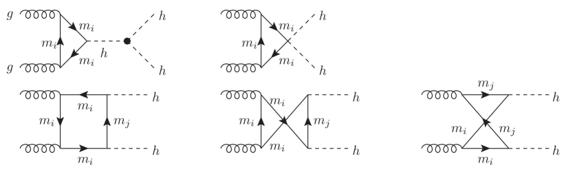
Figure 1: Generic Feynman diagrams contributing to $gg\to hh$ at LO, with $n$ novel fermionic resonances, the top and the bottom quark with masses $m_{i}$ ($i=1,...,n,t,b$). The index $j$ is introduced to indicate where different fermions can contribute in the loop.

Besides the new 2-Higgs-2-fermion coupling $f\overline{f}hh$ the additional top and bottom partners in the loops have to be taken into account. These lead also to new box diagrams involving off-diagonal Yukawa couplings, with, respectively, the top and its heavy charge-2/3 partners or the bottom and its heavy partners of charge $-1/3$. The hadronic cross section is obtained by convolution with the parton distribution functions $f_{g}$ of the gluon in the proton,

$$\sigma(pp\to hh+X)=\int_{\tau_{0}}^{1}d\tau\int_{\tau}^{1}\frac{dx}{x}\,f_{g}(x,\mu_{F})\,f_{g}(\tau/x,\mu_{F})\,\hat{\sigma}_{\text{LO}}(\tau s)\;,$$ (14)

where $s$ denotes the squared hadronic c.m. energy, $\mu_{F}$ the factorization scale and

$$\tau_{0}=\frac{4m_{h}^{2}}{s}$$ (15)

in terms of the Higgs boson mass $m_{h}$. The partonic LO cross section can be cast into the form

$$\hat{\sigma}_{\text{LO}}(gg\to hh)\!\! = \!\!\frac{\alpha_{s}^{2}(\mu_{R})}{1024(2\pi)^{3}\hat{s}^{2}}\int_{\hat{t}_{-}}^{\hat{t}_{+}}d\hat{t}\left[\Big{|}\sum_{q=t,b}\left(F_{\Delta}^{\text{LO}}+F_{\Box}^{\text{LO}}\right)\Big{|}^{2}+\Big{|}\sum_{q=t,b}G_{\Box}^{\text{LO}}\Big{|}^{2}\right]\;,$$ (16)

with the strong coupling constant $\alpha_{s}$ at the renormalization scale $\mu_{R}$. We have introduced the Mandelstam variables

$$\hat{s}=\tau s=Q^{2}\;,\quad\hat{t}=m_{h}^{2}-\frac{Q^{2}(1-\beta\cos\theta)}{2}\quad\mbox{and}\quad\hat{u}=m_{h}^{2}-\frac{Q^{2}(1+\beta\cos\theta)}{2}\;,$$ (17)

in terms of the scattering angle $\theta$ in the partonic c.m. system with the invariant Higgs pair mass $Q$ and the relative velocity

$$\beta=\sqrt{1-\frac{4m_{h}^{2}}{Q^{2}}}\;.$$ (18)

The integration limits at $\cos\theta=\pm 1$ are given by

$$\hat{t}_{\pm}=m_{h}^{2}-\frac{Q^{2}(1\mp\beta)}{2}\;.$$ (19)

The form factors read

$$F_{\Delta}^{\text{LO}} =\sum_{i=1}^{n_{q}}C_{i,\Delta}F_{\Delta}(m_{i})$$ (20)

$$F_{\Box}^{\text{LO}} =\sum_{i=1}^{n_{q}}\sum_{j=1}^{n_{q}}\left(g_{h\overline{q}_{i}q_{j}}^{2}F_{\Box}(m_{i},m_{j})+g_{h\overline{q}_{i}q_{j},5}^{2}F_{\Box,5}(m_{i},m_{j})\right)$$ (21)

$$G_{\Box}^{\text{LO}} =\sum_{i=1}^{n_{q}}\sum_{j=1}^{n_{q}}\left(g_{h\overline{q}_{i}q_{j}}^{2}G_{\Box}(m_{i},m_{j})+g^{2}_{h\overline{q}_{i}q_{j},5}G_{\Box,5}(m_{i},m_{j})\right)\;.$$ (22)

The triangle and box form factors $F_{\Delta}$, $F_{\Box}$, $F_{\Box,5}$, $G_{\Box}$ and $G_{\Box,5}$ can be found in the appendices of [74, 105]. The sum runs up to $n_{t}=5$ for the top quark and its charge-2/3 partners and up to $n_{b}=4$ in the bottom sector. The couplings are defined as

$$g_{h\overline{q}_{i}q_{j}}=\frac{1}{2}(G_{hqq,ij}+G_{hqq,ji})\;,\qquad g_{h\overline{q}_{i}q_{j},5}=\frac{1}{2}(G_{hqq,ji}-G_{hqq,ij})$$ (23)

and

$$g_{hh\overline{q}_{i}q_{j}}=(G_{hhqq,ij}+G_{hhqq,ji})\;,$$ (24)

where $G_{hqq,ij}$ and $G_{hhqq,ij}$ denote the ($i$th,$j$th) matrix elements of the coupling matrices in Eq. (62) of the appendix. The triangle factor $C_{i,\Delta}$ reads in the MCHM10

$$C_{i,\Delta}=\frac{g_{hhh}g_{h\overline{q}_{i}q_{i}}}{Q^{2}-m_{h}^{2}+im_{h}\Gamma_{h}}+g_{hh\overline{q}_{i}q_{i}}\quad\mbox{with}\quad g_{hhh}=\frac{3m_{h}^{2}}{v}\frac{1-2\xi}{\sqrt{1-\xi}}\;,$$ (25)

as given in the MCHM5. In the SM and in the composite Higgs models MCHM4 and MCHM5 involving solely the Higgs non-linearities and no heavy fermionic resonances, no sum over heavy top and bottom partners contributes and only a sum over the top and bottom running in the loop has to be performed, i.e. $n_{t}=n_{b}=1$, with $m_{i}=m_{j}=m_{q}$ and $q=t,b$, and hence also

$$g_{h\overline{q}_{i}q_{j},5}=0\qquad\mbox{for SM, MCHM4 and MCHM5.}$$ (26)

The Yukawa couplings read

$$g_{h\overline{q}q}^{\text{SM}}=\frac{m_{q}}{v}\;,\quad g_{h\overline{q}q}^{\text{MCHM4}}=g_{h\overline{q}q}^{\text{SM}}\,\sqrt{1-\xi}\qquad\mbox{and}\qquad g_{h\overline{q}q}^{\text{MCHM5}}=g_{h\overline{q}q}^{\text{SM}}\,\frac{1-2\xi}{\sqrt{1-\xi}}\;,$$ (27)

and for the 2-Higgs-2-fermion coupling we have

$$g_{hh\overline{q}q}=0\qquad\mbox{in the SM and}\qquad g_{hh\overline{q}q}^{\text{MCHM4}}=-\xi\,\frac{m_{q}}{v^{2}}\quad\mbox{and}\quad g_{hh\overline{q}q}^{\text{MCHM5}}=-4\xi\,\frac{m_{q}}{v^{2}}\;,$$ (28)

while the Higgs self-coupling becomes

$$g_{hhh}^{\text{SM}}=\frac{3m_{h}^{2}}{v}\;,\quad g_{hhh}^{\text{MCHM4}}=g_{hhh}^{\text{SM}}\,\sqrt{1-\xi}\qquad\mbox{and}\qquad g_{hhh}^{\text{MCHM5}}=g_{hhh}^{\text{SM}}\,\frac{1-2\xi}{\sqrt{1-\xi}}\;.$$ (29)

The Feynman diagrams contributing to Higgs pair production at NLO QCD are shown in Fig. 2. The blob in the figure marks the effective vertices of gluons to Higgs boson(s). The first three Feynman diagrams show the virtual contributions. The remaining Feynman diagrams of Fig. 2 display the real corrections generically ordered by the initial states $gg$, $gq$ and $q\overline{q}$.

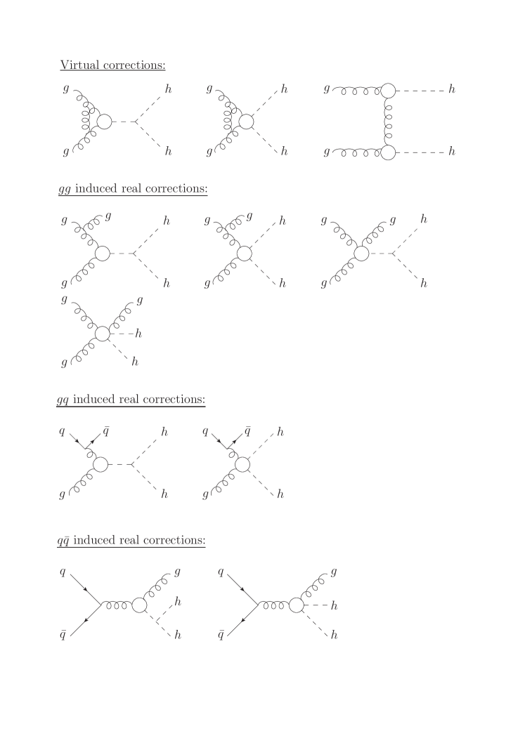
Figure 2: Generic Feynman diagrams contributing to the NLO QCD corrections to $gg\to hh$.

At NLO the cross section is then given by

$$\sigma_{\text{NLO}}(pp\to hh+X)=\sigma_{\text{LO}}+\Delta\sigma_{\text{virt}}+\Delta\sigma_{gg}+\Delta\sigma_{gq}+\Delta\sigma_{q\overline{q}}\,.$$ (30)

The individual contributions in Eq. (30) read

$$\sigma_{\text{LO}} = \int_{\tau_{0}}^{1}d\tau\,\frac{d{\cal L}^{gg}}{d\tau}\,\hat{\sigma}_{\text{LO}}(Q^{2}=\tau s)$$ (31)

$$\Delta\sigma_{\text{virt}} = \frac{\alpha_{s}(\mu_{R})}{\pi}\int_{\tau_{0}}^{1}d\tau\,\frac{d{\cal L}^{gg}}{d\tau}\,\hat{\sigma}_{\text{LO}}(Q^{2}=\tau s)\,C$$ (32)

$$\Delta\sigma_{gg} = \frac{\alpha_{s}(\mu_{R})}{\pi}\int_{\tau_{0}}^{1}d\tau\,\frac{d{\cal L}^{gg}}{d\tau}\int_{\tau_{0}/\tau}^{1}\frac{dz}{z}\,\hat{\sigma}_{\text{LO}}(Q^{2}=z\tau s)\left\{-zP_{gg}(z)\log\frac{\mu_{F}^{2}}{\tau s}\right.$$ (33)

$$\hskip 56.9055pt\left.-\frac{11}{2}(1-z)^{3}+6[1+z^{4}+(1-z)^{4}]\left(\frac{\log(1-z)}{1-z}\right)_{+}\right\}$$

$$\Delta\sigma_{gq} = \frac{\alpha_{s}(\mu_{R})}{\pi}\int_{\tau_{0}}^{1}d\tau\,\sum_{q,\overline{q}}\frac{d{\cal L}^{gq}}{d\tau}\int_{\tau_{0}/\tau}^{1}\frac{dz}{z}\,\hat{\sigma}_{\text{LO}}(Q^{2}=z\tau s)\left\{-\frac{z}{2}P_{gq}(z)\log\frac{\mu_{F}^{2}}{\tau s(1-z)^{2}}\right.$$ (34)

$$\left.\hskip 142.26378pt+\frac{2}{3}z^{2}-(1-z)^{2}\right\}$$

$$\Delta\sigma_{q\overline{q}} = \frac{\alpha_{s}(\mu_{R})}{\pi}\int_{\tau_{0}}^{1}d\tau\,\sum_{q}\frac{d{\cal L}^{q\overline{q}}}{d\tau}\int_{\tau_{0}/\tau}^{1}\frac{dz}{z}\,\hat{\sigma}_{\text{LO}}(Q^{2}=z\tau s)\,\frac{32}{27}(1-z)^{3}\;,$$ (35)

with the Altarelli-Parisi splitting functions given by [106]

$$P_{gg}(z) = 6\left\{\left(\frac{1}{1-z}\right)_{+}+\frac{1}{z}-2+z(1-z)\right\}+\frac{33-2N_{F}}{6}\delta(1-z)$$

$$P_{gq}(z) = \frac{4}{3}\frac{1+(1-z)^{2}}{z}\;,$$ (36)

and $N_{F}=5$ in our case. The real corrections $\Delta\sigma_{gg}$, $\Delta\sigma_{gq}$ and $\Delta\sigma_{q\overline{q}}$ have straightforwardly been obtained from Ref. [4] by replacing the LO cross section of the SM with the LO cross section for composite Higgs models. The calculation of $\Delta\sigma_{\text{virt}}$ is a bit more involved. While the first two diagrams factorize from the LO cross section and can hence directly be taken over from the SM, the third diagram in Fig. 2 does not factorize and needs to be recalculated for the composite Higgs case. The virtual coefficient $C$ is then found to be

$$\begin{split}C=&\pi^{2}+\frac{11}{2}+\frac{33-2N_{F}}{6}\log\frac{\mu_{R}^{2}}{Q^{2}}\\ +&\text{Re}\frac{\int_{\hat{t}_{-}}^{\hat{t}_{+}}d\hat{t}\,\frac{4}{9}(g_{hgg}^{\text{eff}})^{2}\,\biggl{\{}\left(F_{\Delta}^{\text{LO}}+F_{\Box}^{\text{LO}}\right)-\frac{p_{T}^{2}}{2\hat{t}\hat{u}}(Q^{2}-2m_{h}^{2})\,G_{\Box}^{\text{LO}}\biggr{\}}}{\int_{\hat{t}_{-}}^{\hat{t}_{+}}d\hat{t}\,\left[\Big{|}\sum_{q=t,b}\left(F_{\Delta}^{\text{LO}}+F_{\Box}^{\text{LO}}\right)\Big{|}^{2}+\Big{|}\sum_{f=t,b}G_{\Box}^{\text{LO}}\Big{|}^{2}\right]}\end{split}$$ (37)

with

$$p_{T}^{2}=\frac{(\hat{t}-m_{h}^{2})(\hat{u}-m_{h}^{2})}{Q^{2}}-m_{h}^{2}\,.$$ (38)

The first line in Eq. (37) corresponds to the NLO contribution from the first two diagrams in Fig. 2, while the second line corresponds to the NLO contribution from the third diagram of Fig. 2. The factor $(g_{hgg}^{\text{eff}})^{2}$ stems from the two effective Higgs-gluon-gluon vertices in diagram 3 of Fig. 2. This vertex is obtained by integrating out all heavy loop particles in the loop-induced Higgs coupling to gluons defined in Eq. (6) with $g_{hgg}\equiv g_{hgg}^{\text{eff}}$ and

$$g_{hgg}^{\text{eff}}=\left(\sum_{i=1}^{n_{t}}\frac{g_{h\overline{q}_{i}q_{i}}v}{m_{i}}+\sum_{i=1}^{n_{\tilde{b}}}\frac{g_{h\overline{q}_{i}q_{i}}v}{m_{i}}\right)\,.$$ (39)

The first term is the sum over the normalized top quark and top partner couplings and the second term the sum over the normalized bottom partner couplings to the Higgs boson, excluding consistently the light bottom quark contribution from the loop. The composite Higgs cross sections for MCHM4, MCHM5 and for the composite Higgs model with heavy top and bottom partners, including the NLO corrections have been implemented in HPAIR [107]. In order to exemplify the impact of the NLO QCD corrections, we consider the simple case with the pure Higgs non-linearities only and the fermions transforming in the fundamental representation, i.e. the benchmark model MCHM5, see Table 1. The coupling $g_{hgg}^{\text{eff}}$ then reduces to $g_{hgg}^{\text{MCHM5}}=(1-2\xi)/\sqrt{1-\xi}$ and the remaining couplings are given in Eqs. (26)-(29).

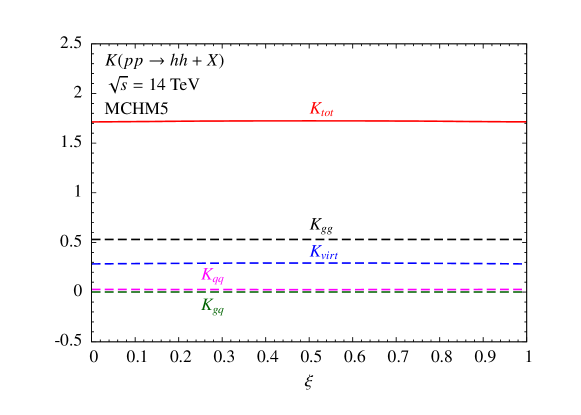
Figure 3: $K$-factors for the $pp\to hh+X$ cross section with $m_{h}=125$ GeV in MCHM5 as a function of $\xi$ for the scale choice $\mu_{F}=\mu_{R}=m_{hh}/2$ and the c.m. energy $\sqrt{s}=14$ TeV. The dashed lines show the individual contributions of the virtual contributions and the real corrections according to their initial states.

We define the $K$-factors for the total cross section and the individual contributions as

$$K=\frac{\sigma_{NLO}}{\sigma_{LO}}\qquad\mbox{and}\qquad K_{i}=\frac{\Delta\sigma_{i}}{\sigma_{LO}}\;,\qquad i=\text{virt},gg,gq,q\overline{q}\;.$$ (40)

The cross section at LO is computed with the full quark mass dependences. As the NLO cross section in the LET approximation only includes top quark contributions, at LO we consistently neglect also the bottom quark contributions, which in the SM amount to 1% for a 125 GeV Higgs boson. The c.m. energy $\sqrt{s}=14$ TeV and the top and bottom quark mass are set to $m_{t}=173.2$ GeV and $m_{b}=4.75$ GeV, respectively. The cross sections are computed with the MSTW2008 PDF set [108]. The strong coupling constant is evaluated at the corresponding loop order with

$$\alpha_{s}^{\text{LO}}(M_{Z})=0.13939\qquad\mbox{and}\qquad\alpha_{s}^{\text{NLO}}(M_{Z})=0.12018\;.$$ (41)

The renormalization and factorization scales are set to $\mu_{R}=\mu_{F}=m_{hh}/2$, where $m_{hh}$ denotes the invariant Higgs pair mass. Figure 3 displays the results for the $K$-factors for the MCHM5 as a function of $\xi$. The solid line shows the total $K$-factor, the dashed lines are the individual contributions. As can be inferred from the plot, the real and virtual corrections of the $gg$ initial state make up the bulk of the QCD corrections. The $qg$ and the $q\overline{q}$ initiated real radiation diagrams only lead to a small correction. The $K$-factor is almost independent of $\xi$. In the real corrections, the Born cross section, which shows the only dependence on $\xi$, almost completely drops out numerically. For the virtual contributions some dependence on $\xi$ may be expected. The virtual correction due to the constant term in $C$, i.e. the first line in Eq. (37) does not develop any dependence on $\xi$, however, as it factorizes from the LO cross section. The dependence of $\xi$ can only emerge from the second line in Eq. (37), which, however, is numerically suppressed. This is already the case in the SM, where the corresponding term contributes less than 3% to $\Delta\sigma_{\text{virt}}$. This result also holds true for the case were the heavy quark partners are explicitly included. In composite Higgs models, the NLO QCD corrections to Higgs pair production can hence well be approximated by multiplying the full LO cross section of the composite Higgs model under consideration with the SM $K$-factor.

Figure 3 can also be obtained by using the results of Ref. [89]. Note however, that the effects of heavy top and bottom partners in the effective field theory computation of Ref. [89] have to be added to the top quark contribution, encoded into the Wilson coefficients in front of the operators $hG^{\mu\nu}G_{\mu\nu}$ and $hhG^{\mu\nu}G_{\mu\nu}$.

4 Numerical Analysis of New Physics Effects in Higgs Pair Production via Gluon Fusion

Having derived the NLO QCD corrections, we can now turn to the analysis of NP effects in Higgs pair production. We assume that no NP is found before Higgs pair production becomes accessible. This means that we require deviations in the Higgs boson couplings with respect to the SM to be smaller than the projected sensitivities of the coupling measurements at an integrated luminosity of $300\;\text{fb}^{-1}$ and $3000\;\text{fb}^{-1}$, respectively. For the projected sensitivities we take the numbers reported in Ref. [109]. Similar numbers can be found in Refs. [110]. In our analysis we focus on the most promising final states, given by $b\overline{b}\gamma\gamma$ and $b\overline{b}\tau^{+}\tau^{-}$ [13, 8, 9, 10].

We call Higgs pair production to be sensitive to NP if the difference between the number of signal events $S$ in the considered NP model and the corresponding number $S_{SM}$ in the SM exceeds a minimum of 3 statistical standard deviations, i.e.

$$S_{SM}+\beta\sqrt{S_{SM}}\leq S\hskip 28.45274pt\text{or}\hskip 28.45274ptS_{SM}-\beta\sqrt{S_{SM}}\geq S$$ (42)

with $\beta=3$ for a $3\sigma$ deviation. The signal events are obtained as

$$S=\sigma\cdot BR\cdot L\cdot A\;,$$ (43)

where $BR$ denotes the branching ratio into the respective final states, $L$ the integrated luminosity and $A$ the acceptance due to cuts applied on the cross section. The acceptances have been extracted from Ref. [13] for the $b\overline{b}\gamma\gamma$ and $b\overline{b}\tau^{+}\tau^{-}$ final states. The acceptance for the BSM signal only changes slightly, as we explicitly checked.

In specific models, the correlations of the couplings will lead to stronger bounds on the parameters. In particular in the MCHM4 and MCHM5 as introduced in section 2, the only new parameter is $\xi$. The value of $\xi$ can hence strongly be restricted by Higgs coupling measurements [111]. Based on the data for a c.m. energy of $\sqrt{s}=7$ and 8 TeV at an integrated luminosity of 4.6-4.8 fb^-1 and 20.3 fb^-1, respectively, ATLAS observes a 95% C.L. upper limit of $\xi<0.12$ in the MCHM4 and of $\xi<0.15$ in the MCHM5 [112]. This restricts the gluon fusion cross section for the MCHM4 to the range $40.06\;\text{fb}\leq\sigma_{\text{MCHM4}}\leq 44.55\;\text{fb}$ and for the MCHM5 to $40.06\;\text{fb}\leq\sigma_{\text{MCHM5}}\leq 89.26\;\text{fb}$. The value $\sigma=40.06\;\text{fb}$ corresponds to the SM cross section at NLO QCD for $m_{t}=173.2\;\text{GeV}$ and hence the MCHM4/MCHM5 value for $\xi=0$. For the high luminosity options at the LHC we apply the projected estimates for the parameter $\xi$ given in Ref. [109],

$$\begin{array}[]{lll}\int{\cal L}=300\mbox{ fb}^{-1}:&\mbox{MCHM4:}&0.076\\ &\mbox{MCHM5:}&0.068\\[2.84544pt] \int{\cal L}=3000\mbox{ fb}^{-1}:&\mbox{MCHM4:}&0.051\\ &\mbox{MCHM5:}&0.015\end{array}$$ (48)

Based on these estimates, we give in Table 2 the maximal values for the cross section times branching ratio. In the fourth and sixth columns we report whether the process within MCHM4, respectively, MCHM5 can be distinguished from the SM cross section by more than $3\sigma$ according to the criteria given in Eq. (42) for $\beta=3$. In the check of Eq. (42) we took into account the slight change in the acceptance of the signal rate for the composite Higgs models. Due to the coupling modifications and the new diagram from the 2-Higgs-2-fermion coupling the applied cuts in the analysis of Ref. [13] affect the cross section in a slightly different way.

		$\sigma_{b\overline{b}\gamma\gamma}$ [fb]	$\Delta_{3\sigma}$	$\sigma_{b\overline{b}\tau^{+}\tau^{-}}$ [fb]	$\Delta_{3\sigma}$
	$\xi=0.12$ (LHC20.3)	0.119	no	3.26	no
MCHM4	$\xi=0.076$ (LHC300)	$0.114$	no	3.13	no
	$\xi=0.051$ (LHC3000)	0.112	no	3.07	no
	$\xi=0.15$ (LHC20.3)	0.315	yes	5.35	yes
MCHM5	$\xi=0.068$ (LHC300)	$0.175$	no	3.96	no
	$\xi=0.015$ (LHC3000)	$0.119$	no	3.14	no

Table 2: Values of the cross section times branching ratio in the MCHM4 and MCHM5 for the maximal allowed values of $\xi$ at $95\%$ C.L. [112] and for the projected values at $\int\mathcal{L}=300\;\text{fb}^{-1}$ and $\int\mathcal{L}=3000\;\text{fb}^{-1}$ of Ref. [109]. The fourth and sixth columns decide whether the Higgs production cross section will develop a deviation to the SM Higgs pair production cross section of more than $3\sigma$ according to the criteria of Eq. (42).

The table shows, that with the projected precision on $\xi$ at high luminosities Higgs pair production in both MCHM4 and MCHM5 leads to cross sections too close to the SM value to be distinguishable from the SM case. Although with the present bounds on $\xi$ Higgs pair production in MCHM5 differs by more than 3$\sigma$ from the SM prediction, the corresponding cross section is too small to be measurable, so that first signs of NP through this process are precluded.

5 Numerical Analysis for MCHM10

We consider the MCHM10 with one multiplet of fermionic resonances below the cut-off. In this model, with more than one parameter determining the Higgs coupling modifications, there is more freedom and a larger allowed parameter space (see Ref. [102] for a thorough analysis). This implies, that the sensitivity on the Higgs couplings is less constrained. The numbers of the projected sensitivities are taken from Table I in Ref. [109]. Additionally, we need to take into account the bounds from the direct searches for new fermions. Currently, exotic new fermions with charge 5/3 are excluded up to masses of $m_{\chi}\leq 840\;\text{GeV}$ [113], bottom partners up to masses of $m_{B}\leq 900\;\text{GeV}$ [114] and top partners with masses of $m_{T}\leq 950\;\text{GeV}$ [115]. Note that the latter two limits on the masses depend on the branching ratios of the bottom and top partner, respectively. These limits are based on pair production of the new heavy fermions. First studies for single production of a new vector-like fermion were performed in Refs. [116] and can potentially be more important at large energies [117] but are more model-dependent. Due to this model dependence it is difficult to estimate the LHC reach on single production for our case. Hence we will only use the estimated reach on new vector-like fermions in pair production. In Refs. [118, 119] the potential reach of the LHC for charged-2/3 fermions, depending on their branching ratios is estimated. Following [119] we use the reach $m_{T}\lesssim 1.3\text{ TeV}$ for $\int\mathcal{L}=300\text{ fb}^{-1}$ and $m_{T}\lesssim 1.5\text{ TeV}$ for $\int\mathcal{L}=3000\text{ fb}^{-1}$. The potential reach for bottom partners is $m_{B}\lesssim 1\text{ TeV}$ for $\int\mathcal{L}=300\text{ fb}^{-1}$ and $m_{B}\lesssim 1.5\text{ TeV}$ for $\int\mathcal{L}=3000\text{ fb}^{-1}$ [120]. We estimate the additional sensitivity for the reach of exotic new fermions by multiplying the excluded cross section at $\sqrt{s}=8$ TeV with [121]

$$r=\sqrt{\frac{\sigma_{BKG}(14\text{ TeV})}{\sigma_{BKG}(8\text{ TeV})}\frac{L_{LHC8}}{L_{LHC14}}}\;,$$ (49)

where $L_{\text{LHC8}}$ and $L_{\text{LHC14}}$ denote the integrated luminosities of the LHC run at $\sqrt{s}=8$ and 14 TeV, respectively. This implies a reach of $m_{\chi}\approx 1370\text{ GeV}$ at $\int\mathcal{L}=300\text{ fb}^{-1}$ and $m_{\chi}\approx 1550\text{ GeV}$ at $\int\mathcal{L}=3000\text{ fb}^{-1}$. For the background estimate we only considered the dominant background $t\overline{t}W^{\pm}$ [122]. The background cross section was computed with MadGraph5 [123]. Although the assumption of stronger projections on the reach of new fermion masses of up to 2 TeV [124] will lead to a reduced number of points allowed by the constraints we are imposing, it will not change our final conclusion, as we checked explicitly. Note also that in composite Higgs models there is a connection between the Higgs boson mass and the fermionic resonances [125, 126]. Reference [126] finds that the mass of the lightest top partner $m_{T_{\text{lightest}}}$ should be lighter than

$$m_{T_{\text{lightest}}}\lesssim\frac{m_{h}\pi v}{m_{t}\sqrt{N_{c}}\sqrt{\xi}}\;,$$ (50)

with $N_{c}=3$ denoting the number of colors. This bound automatically eliminates large values of $\xi$. In our analysis we allow for finetuning, hence small values of $\xi$, and we will not apply this bound.

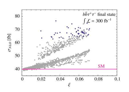
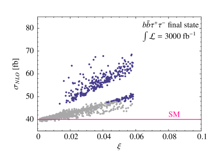
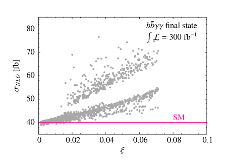
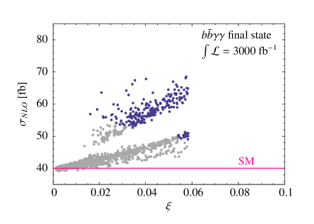
Figure 4: The NLO gluon fusion cross section into Higgs pairs in MCHM10 for a scan over $\xi$, $y$, $\sin\phi_{L}$ and $M_{10}$. All points pass the EWPTs and, for the respective luminosity, fulfill the projected direct search limits for new fermionic resonances at the LHC and allow only for deviations in the Higgs boson couplings that are smaller than the according expected sensitivity at the LHC. The blue points indicate that the composite Higgs pair production cross section can be distinguished from the SM one at 3$\sigma$ in the $b\overline{b}\tau^{+}\tau^{-}$ final state (upper) and $b\overline{b}\gamma\gamma$ final state (lower) at an integrated luminosity $L=300\text{ fb}^{-1}$ (left) and $L=3000\text{ fb}^{-1}$ (right). The grey points cannot be distinguished from the SM at 3$\sigma$. The pink line is the SM prediction for the gluon fusion cross section at NLO.

For the analysis we performed a scan over the parameter space of the model by varying the parameters in the range

$$0\leq\xi\leq 1\,,\hskip 14.22636pt0<\sin\phi_{L}\leq 1\,,\hskip 14.22636pt|y|<4\pi\,,\hskip 14.22636pt0\leq M_{10}\leq 10\text{ TeV}\,.$$ (51)

We excluded points that do not fulfill $|V_{tb}|>0.92$ [127] and the electroweak precision tests (EWPTs) at 99% C.L. using the results of Ref. [102].

In Fig. 4 we show the NLO Higgs pair production cross section via gluon fusion as a function of $\xi$. The color code in the plots indicates whether the points are distinguishable from the SM according to the criteria given in Eq. (42), with the blue points being distinguishable and the grey points not. The upper plots are for the $b\overline{b}\tau^{+}\tau^{-}$ final state, the lower plots for the $b\overline{b}\gamma\gamma$ final state, for $\int\mathcal{L}=300\text{ fb}^{-1}$ (left) and $\int\mathcal{L}=3000\text{ fb}^{-1}$ (right), respectively. The upper branch in the plots corresponds to the parameters $y<0$ and $0<R<1$ with $R=(M_{10}+fy/2)/M_{10}$. This means that at LO of the mass matrix expansion in $v/f$, the lightest fermion partner originates from the $SU(2)$ bi-doublet. The lower branch corresponds to the cases $y<0$ and $R<0$ as well as $y>0$ implying $R>1$.

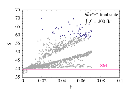
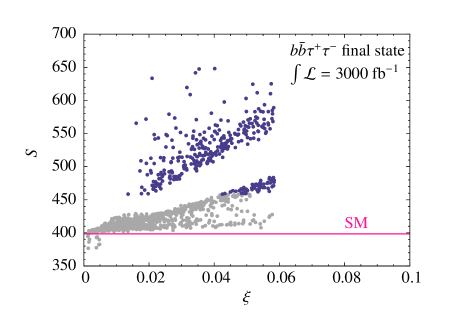
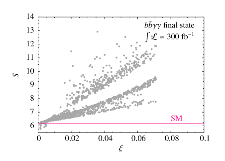
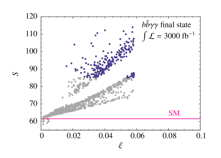
Figure 5: Number of signal events $S=\sigma_{NLO}\cdot 2\cdot\mbox{BR}(h\to X)\cdot\mbox{BR}(h\to Y)\cdot A\cdot L$ for NLO Higgs pair production in the final states $X=b\overline{b}$, $Y=\tau^{+}\tau^{-}$ (upper) and $X=b\overline{b}$, $Y=\gamma\gamma$ (lower) for an integrated luminosity of $L=300$ fb^-1 (left) and $L=3000$ fb^-1 (right), after multiplication with the individual acceptance $A$ of the applied cuts, for the parameter points given in Fig. 4. The colour code is the same and the pink line refers to the NLO signal rate in the SM.

The plots only show points for which we cannot see new physics anywhere else meaning we require that their deviations in the Higgs couplings that can be tested at the LHC are smaller than the expected sensitivities and that the masses of the new fermionic resonances are above the estimated reach of direct searches. The requirement for only small deviations in the Higgs couplings directly restricts the possible values of $\xi$ to be smaller than 0.071 and 0.059 for $\int\mathcal{L}=300\text{ fb}^{-1}$ and $\int\mathcal{L}=3000\text{ fb}^{-1}$, respectively. The value of $\xi$ is restricted more strongly than in the MCHM4 due to the different coupling modifications, which, considering pure non-linearities, are for the Higgs-fermion couplings $(1-2\xi)/\sqrt{1-\xi}$ in MCHM10 and $\sqrt{1-\xi}$ in the MCHM4. Although the interplay of the various additional parameters in MCHM10 allows for some tuning in the Higgs-bottom (and also Higgs-top) coupling, this is not the case for the Higgs-tau coupling. Comparing the MCHM10 with the MCHM5, the Higgs-fermion couplings are modified in the same way, barring the effects from the additional fermions. The increased number of parameters due to the heavy fermions, however, allows for more freedom to accommodate the data, so that here the constraint is weaker in the MCHM10. The plots show that at $\int\mathcal{L}=300\text{ fb}^{-1}$ we cannot expect to discover NP for the first time in Higgs pair production in the $b\overline{b}\gamma\gamma$ final state, while in the $b\overline{b}\tau^{+}\tau^{-}$ final state NP could show up for the first time in Higgs pair production. For $\int\mathcal{L}=3000\text{ fb}^{-1}$, we could find both in the $b\overline{b}\tau^{+}\tau^{-}$ and the $b\overline{b}\gamma\gamma$ final state points which lead to large enough deviations from the SM case to be sensitive to NP for the first time in Higgs pair production. These results can be explained with the increased signal rate in the cases that are sensitive, as can be inferred from Fig. 5. The plots show for the parameter points displayed in Fig. 4 the corresponding number of signal events for Higgs pair production in the $b\overline{b}\tau^{+}\tau^{-}$ and $b\overline{b}\gamma\gamma$ final states, respectively, after applying the acceptance of the cuts and multiplication with the two options of integrated luminosity. The blue points clearly deviate by more than 3$\sigma$ from the SM curve.

6 Invariant Mass Distributions

Finally, in this section we discuss NP effects in invariant Higgs mass distributions. The measurement of distributions can give information on anomalous couplings [69] or the underlying ultraviolet source of NP [128]. Even though they are difficult to be measured due to the small numbers of signal events, they are important observables for the NP search. In the following we will show the impact of composite Higgs models on the distributions.

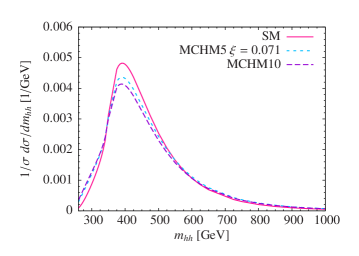
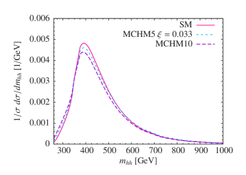
Figure 6: Normalized invariant mass distributions at NLO QCD for the SM (pink solid) and left: MCHM5 with $\xi=0.071$ (blue dotted) and the MCHM10 with fermionic resonances for the parameter choice $\xi=0.071$, $y=-7.292$, $\sin\phi_{L}=0.551$ and $R=0.615$ (violet dashed); right: MCHM5 with $\xi=0.033$ (blued dotted) and the MCHM10 parameter choice $\xi=0.033$, $y=-10.898$, $\sin\phi_{L}=0.895$ and $R=0.181$ (violet dashed).

Figure 6 (left) shows the normalized invariant mass distributions for the MCHM5 with $\xi=0.071$ (blue dotted) and the MCHM10 with one multiplet of fermionic resonances for the parameter choice $\xi=0.071$, $y=-7.292$, $\sin\phi_{L}=0.551$ and $R=0.615$ (violet dashed) compared to the SM case (pink solid). In the right plot we show the same quantity, but for the MCHM5 with $\xi=0.033$ (blue dotted) and the MCHM10 parameters $\xi=0.033$, $y=-10.898$, $\sin\phi_{L}=0.895$ and $R=0.181$ (violet dashed) again compared to the SM (pink solid). The cross sections are computed at NLO. Note, however, that the shape of the invariant mass distributions hardly changes from LO to NLO, since in the LET approximation the LO cross section mainly factorizes from the NLO contributions, as discussed in section 3. The parameters have been chosen such that in the left plot we allow for a larger value of $\xi$, while the mass of the lightest top partner of $m_{T,\text{lightest}}=5441\text{ GeV}$ is much larger than compared to the case shown in the right plot with $m_{T,\text{lightest}}=1636\text{ GeV}$. As can be inferred from these plots, the largest effect on the distributions originates from the pure non-linearities, i.e. the value of $\xi$, while the influence of the fermionic resonances on the shape of the invariant mass distributions is small. Note also that the main effect on the distributions emerges from the new $t\overline{t}hh$ coupling.

7 Conclusions

We presented the NLO QCD corrections to Higgs pair production via gluon fusion in the large quark mass approximation in composite Higgs models with and without new heavy fermionic resonances below the UV cut-off. We found that the $K$-factor of $\sim 1.7$ is basically independent of the value of $\xi$ and of the details of the fermion spectrum, as the LO cross section dominantly factorizes. The $K$-factor can hence directly be taken over from the SM to a good approximation. The size of the absolute value of the cross section, however, sensitively depends on the Higgs non-linearities and on the fermion spectrum.

With the results of our NLO calculation, we furthermore addressed the question of whether NP could emerge for the first time in Higgs pair production, taking into account the constraints on the Higgs couplings to SM particles and from direct searches for new heavy fermions. We focused on composite Higgs models and found that in simple models where only the Higgs non-linearities are considered, we cannot expect to be sensitive to NP for the first time in Higgs pair production. In models with a multiplet of new fermions below the cut-off, it turned out that there are regions where NP could indeed be seen for the first time in Higgs pair production. The subsequent study of the NLO invariant mass distributions demonstrated, that while there is some sensitivity to the Higgs non-linearities mainly due to the new 2-Higgs-2-fermion coupling, the effect of the heavy fermions on the shape of the distributions is much weaker. By applying optimized cuts the sensitivity to new physics effects may possibly be increased in future.

Acknowledgments

This work is supported in part by the Research Executive Agency (REA) of the European Union under Grant No. PITN-GA-2012-316704 (Higgstools).

Appendix

Appendix A Masses and Couplings

In the following we give the mass and coupling matrices for the composite Higgs model MCHM10 with heavy top and fermion partners, needed in the gluon fusion process into Higgs pairs. With the abbreviations

$$s_{H}\equiv\sin(H/f)\;,\qquad c_{H}\equiv\cos(H/f)$$ (52)

and

$$\tilde{m}_{a}\equiv\frac{1}{4}fys_{H}^{2}+M_{10}\;,\hskip 28.45274pt\tilde{m}_{b}\equiv\frac{1}{2}fy(1-\frac{1}{2}s_{H}^{2})+M_{10}\;,\hskip 28.45274pt\tilde{m}_{c}\equiv\frac{1}{2}fyc_{H}^{2}+M_{10}\;,$$ (53)

the terms bilinear in the quark fields of Eq. (12) read

$$-\mathcal{L}_{m_{t}}=\overline{\left(\begin{array}[]{c}t_{L}\\ u_{L}\\ u_{1L}\\ t_{4L}\\ T_{4L}\end{array}\right)}\left(\begin{array}[]{ccccc}0&0&0&0&\lambda_{q}\\ 0&\tilde{m}_{a}&-\frac{1}{4}fys_{H}^{2}&-\frac{1}{4}fyc_{H}s_{H}&-\frac{1}{4}fyc_{H}s_{H}\\ \lambda_{t}&-\frac{1}{4}fys_{H}^{2}&\tilde{m}_{a}&\frac{1}{4}fyc_{H}s_{H}&\frac{1}{4}fyc_{H}s_{H}\\ 0&-\frac{1}{4}fyc_{H}s_{H}&\frac{1}{4}fyc_{H}s_{H}&\tilde{m}_{b}&-\frac{1}{4}fys_{H}^{2}\\ 0&-\frac{1}{4}fyc_{H}s_{H}&\frac{1}{4}fyc_{H}s_{H}&-\frac{1}{4}fys_{H}^{2}&\tilde{m}_{b}\end{array}\right)\left(\begin{array}[]{c}t_{R}\\ u_{R}\\ u_{1R}\\ t_{4R}\\ T_{4R}\end{array}\right)+h.c.\;,$$ (54)

$$-\mathcal{L}_{m_{b}}=\overline{\left(\begin{array}[]{c}b_{L}\\ d_{L}\\ d_{1L}\\ d_{4L}\end{array}\right)}\left(\begin{array}[]{cccc}0&0&0&\lambda_{q}\\ 0&\tilde{m}_{a}&-\frac{1}{4}fys_{H}^{2}&fy\frac{c_{H}s_{H}}{2\sqrt{2}}\\ \lambda_{b}&-\frac{1}{4}fys_{H}^{2}&\tilde{m}_{a}&-fy\frac{c_{H}s_{H}}{2\sqrt{2}}\\ 0&fy\frac{c_{H}s_{H}}{2\sqrt{2}}&-fy\frac{c_{H}s_{H}}{2\sqrt{2}}&\tilde{m}_{c}\end{array}\right)\left(\begin{array}[]{c}b_{R}\\ d_{R}\\ d_{1R}\\ d_{4R}\end{array}\right)+h.c.\;,$$ (55)

and

$$-\mathcal{L}_{m_{\chi}}=\overline{\left(\begin{array}[]{c}\chi_{L}\\ \chi_{1L}\\ \chi_{4L}\end{array}\right)}\left(\begin{array}[]{ccc}\tilde{m}_{a}&-\frac{1}{4}fys_{H}^{2}&fy\frac{c_{H}s_{H}}{2\sqrt{2}}\\ -\frac{1}{4}fys_{H}^{2}&\tilde{m}_{a}&-fy\frac{c_{H}s_{H}}{2\sqrt{2}}\\ fy\frac{c_{H}s_{H}}{2\sqrt{2}}&-fy\frac{c_{H}s_{H}}{2\sqrt{2}}&\tilde{m}_{c}\end{array}\right)\left(\begin{array}[]{c}\chi_{R}\\ \chi_{1R}\\ \chi_{4R}\end{array}\right)+h.c.\;.$$ (56)

Shifting the Higgs field in Eqs. (54)–(56), encoded in $s_{H}$ and $c_{H}$, respectively, by its VEV, i.e. $H=\langle H\rangle+h$, leads to the mass matrices $M_{t}$, $M_{b}$ and $M_{\chi}$. They can be diagonalized by a bi-unitary transformation

$$\left(U_{L}^{(t/b/\chi)}\right)^{\dagger}M_{(t/b/\chi)}U_{R}^{(t/b/\chi)}=M_{(t/b/\chi)}^{\text{diag}}\;,$$ (57)

where $U_{L,R}^{(t/b/\chi)}$ denote the transformations that diagonalize the mass matrix in the top, bottom and charge-5/3 ($\chi$) sector, respectively. Expansion of the mass matrices Eqs. (54)–(56) in the interaction eigenstates up to first order in the Higgs field leads to the Higgs coupling matrices $\tilde{G}_{ht\overline{t}}$ to a pair of charge-2/3 quarks and $\tilde{G}_{hb\overline{b}}$ to a quark pair of charge $-1/3$, respectively, given by

$$-\mathcal{L}_{ht\overline{t}}=y\;h\overline{\left(\begin{array}[]{c}t_{L}\\ u_{L}\\ u_{1L}\\ t_{4L}\\ T_{4L}\end{array}\right)}\underbrace{\left(\begin{array}[]{ccccc}0&0&0&0&0\\ 0&\frac{1}{2}s_{H}c_{H}&-\frac{1}{2}s_{H}c_{H}&\frac{1}{4}(2s_{H}^{2}-1)&\frac{1}{4}(2s_{H}^{2}-1)\\ 0&-\frac{1}{2}s_{H}c_{H}&\frac{1}{2}s_{H}c_{H}&\frac{1}{4}(1-2s_{H}^{2})&\frac{1}{4}(1-2s_{H}^{2})\\ 0&\frac{1}{4}(2s_{H}^{2}-1)&\frac{1}{4}(1-2s_{H}^{2})&-\frac{1}{2}s_{H}c_{H}&-\frac{1}{2}s_{H}c_{H}\\ 0&\frac{1}{4}(2s_{H}^{2}-1)&\frac{1}{4}(1-2s_{H}^{2})&-\frac{1}{2}s_{H}c_{H}&-\frac{1}{2}s_{H}c_{H}\end{array}\right)}_{\tilde{G}_{ht\overline{t}}/y}\left(\begin{array}[]{c}t_{R}\\ u_{R}\\ u_{1R}\\ t_{4R}\\ T_{4R}\end{array}\right)_{H=\langle H\rangle}+h.c.\;,$$ (58)

$$-\mathcal{L}_{hb\overline{b}}=y\;h\overline{\left(\begin{array}[]{c}b_{L}\\ d_{L}\\ d_{1L}\\ d_{4L}\end{array}\right)}\underbrace{\left(\begin{array}[]{cccc}0&0&0&0\\ 0&\frac{1}{2}s_{H}c_{H}&-\frac{1}{2}s_{H}c_{H}&\frac{1}{2\sqrt{2}}(1-2s_{H}^{2})\\ 0&-\frac{1}{2}s_{H}c_{H}&\frac{1}{2}s_{H}c_{H}&\frac{1}{2\sqrt{2}}(2s_{H}^{2}-1)\\ 0&\frac{1}{2\sqrt{2}}(1-2s_{H}^{2})&\frac{1}{2\sqrt{2}}(2s_{H}^{2}-1)&-s_{H}c_{H}\end{array}\right)}_{\tilde{G}_{hb\overline{b}}/y}\left(\begin{array}[]{c}b_{R}\\ d_{R}\\ d_{1R}\\ d_{4R}\end{array}\right)_{H=\langle H\rangle}+h.c.\;.$$ (59)

Expansion up to second order in the Higgs field yields the 2-Higgs-2-fermion coupling matrices $\tilde{G}_{hht\overline{t}}$ and $\tilde{G}_{hhb\overline{b}}$, that can be cast into the form

$$-\mathcal{L}_{hht\overline{t}}=\frac{y}{2\,f}\;h\overline{\left(\begin{array}[]{c}t_{L}\\ u_{L}\\ u_{1L}\\ t_{4L}\\ T_{4L}\end{array}\right)}\underbrace{\left(\begin{array}[]{ccccc}0&0&0&0&0\\ 0&(1-2s_{H}^{2})&-(1-2s_{H}^{2})&2s_{H}c_{H}&2s_{H}c_{H}\\ 0&-(1-2s_{H}^{2})&(1-2s_{H}^{2})&-2s_{H}c_{H}&\frac{1}{4}(1-2s_{H}^{2})\\ 0&2s_{H}c_{H}&-2s_{H}c_{H}&-(1-2s_{H}^{2})&-(1-2s_{H}c_{H})\\ 0&2s_{H}c_{H}&2s_{H}c_{H}&-(1-2s_{H}^{2})&-(1-2s_{H}^{2})\end{array}\right)}_{2\,f\,\tilde{G}_{hht\overline{t}}/y}\left(\begin{array}[]{c}t_{R}\\ u_{R}\\ u_{1R}\\ t_{4R}\\ T_{4R}\end{array}\right)_{H=\langle H\rangle}+h.c.\;,$$ (60)

$$-\mathcal{L}_{hb\overline{b}}=\frac{y}{2f}\;h\overline{\left(\begin{array}[]{c}b_{L}\\ d_{L}\\ d_{1L}\\ d_{4L}\end{array}\right)}\underbrace{\left(\begin{array}[]{cccc}0&0&0&0\\ 0&(1-2s_{H}^{2})&-(1-2s_{H}^{2})&-\sqrt{2}s_{H}c_{H}\\ 0&-(1-2s_{H}^{2})&(1-2s_{H}^{2})&\sqrt{2}s_{H}c_{H}\\ 0&-\sqrt{2}s_{H}c_{H}&\sqrt{2}s_{H}c_{H}&-2(1-2s_{H}^{2})\end{array}\right)}_{2\,f\,\tilde{G}_{hhb\overline{b}}/y}\left(\begin{array}[]{c}b_{R}\\ d_{R}\\ d_{1R}\\ d_{4R}\end{array}\right)_{H=\langle H\rangle}+h.c.\;.$$ (61)

The coupling matrices in the mass eigenstate basis are obtained by rotation with the unitary matrices defined in Eq. (57), i.e. ($q=t,b$)

$$(U_{L}^{q})^{\dagger}\tilde{G}_{hq\overline{q}}U_{R}^{q}=G_{hq\overline{q}}\qquad\mbox{and}\qquad(U_{L}^{q})^{\dagger}\tilde{G}_{hhq\overline{q}}U_{R}^{q}=G_{hhq\overline{q}}\;.$$ (62)

References

- [1] G. Aad et al. [ATLAS Collaboration], Phys. Lett. B 716 (2012) 1 [arXiv:1207.7214 [hep-ex]]; G. Aad et al. [ATLAS Collaboration], ATLAS-CONF-2012-162.
- [2] S. Chatrchyan et al. [CMS Collaboration], Phys. Lett. B 716 (2012) 30 [arXiv:1207.7235 [hep-ex]]; S. Chatrchyan et al. [CMS Collaboration], CMS-PAS-HIG-12-045.
- [3] P. W. Higgs, Phys. Rev. Lett. 13 (1964) 508; P. W. Higgs, Phys. Lett. 12 (1964) 132; F. Englert and R. Brout, Phys. Rev. Lett. 13 (1964) 321; G. S. Guralnik, C. R. Hagen and T. W. B. Kibble, Phys. Rev. Lett. 13 (1964) 585; T. W. B. Kibble, Phys. Rev. 155 (1967) 1554.
- [4] S. Dawson, S. Dittmaier and M. Spira, Phys. Rev. D 58 (1998) 115012 [hep-ph/9805244].
- [5] A. Djouadi, W. Kilian, M. Mühlleitner and P. M. Zerwas, Eur. Phys. J. C 10 (1999) 27 [hep-ph/9903229].
- [6] A. Djouadi, W. Kilian, M. Mühlleitner and P. M. Zerwas, Eur. Phys. J. C 10 (1999) 45 [hep-ph/9904287];
- [7] M. M. Mühlleitner, PhD Thesis (2000), DESY Hamburg and University of Hamburg [hep-ph/0008127].
- [8] U. Baur, T. Plehn and D. L. Rainwater, Phys. Rev. D 67 (2003) 033003 [hep-ph/0211224]; U. Baur, T. Plehn and D. L. Rainwater, Phys. Rev. D 68 (2003) 033001 [hep-ph/0304015].
- [9] U. Baur, T. Plehn and D. L. Rainwater, Phys. Rev. Lett. 89 (2002) 151801 [hep-ph/0206024].
- [10] U. Baur, T. Plehn and D. L. Rainwater, Phys. Rev. D 69 (2004) 053004 [hep-ph/0310056].
- [11] M. J. Dolan, C. Englert and M. Spannowsky, JHEP 1210 (2012) 112 [arXiv:1206.5001 [hep-ph]].
- [12] A. Papaefstathiou, L. L. Yang and J. Zurita, Phys. Rev. D 87 (2013) 1, 011301 [arXiv:1209.1489 [hep-ph]].
- [13] J. Baglio, A. Djouadi, R. Gröber, M. M. Mühlleitner, J. Quevillon and M. Spira, JHEP 1304 (2013) 151 [arXiv:1212.5581 [hep-ph]].
- [14] F. Goertz, A. Papaefstathiou, L. L. Yang and J. Zurita, JHEP 1306 (2013) 016 [arXiv:1301.3492 [hep-ph]].
- [15] W. Yao, arXiv:1308.6302 [hep-ph].
- [16] A. J. Barr, M. J. Dolan, C. Englert and M. Spannowsky, Phys. Lett. B 728 (2014) 308 [arXiv:1309.6318 [hep-ph]].
- [17] M. J. Dolan, C. Englert, N. Greiner and M. Spannowsky, Phys. Rev. Lett. 112 (2014) 101802 [arXiv:1310.1084 [hep-ph]].
- [18] V. Barger, L. L. Everett, C. B. Jackson and G. Shaughnessy, Phys. Lett. B 728 (2014) 433 [arXiv:1311.2931 [hep-ph]].
- [19] D. E. Ferreira de Lima, A. Papaefstathiou and M. Spannowsky, JHEP 1408 (2014) 030 [arXiv:1404.7139 [hep-ph]].
- [20] C. Englert, F. Krauss, M. Spannowsky and J. Thompson, Phys. Lett. B 743 (2015) 93 [arXiv:1409.8074 [hep-ph]].
- [21] D. Wardrope, E. Jansen, N. Konstantinidis, B. Cooper, R. Falla and N. Norjoharuddeen, Eur. Phys. J. C 75 (2015) 5, 219 [arXiv:1410.2794 [hep-ph]].
- [22] Q. Li, Z. Li, Q. S. Yan and X. Zhao, Phys. Rev. D 92 (2015) 1, 014015 [arXiv:1503.07611 [hep-ph]].
- [23] C. T. Lu, J. Chang, K. Cheung and J. S. Lee, JHEP 1508 (2015) 133 [arXiv:1505.00957 [hep-ph]].
- [24] M. J. Dolan, C. Englert, N. Greiner, K. Nordstrom and M. Spannowsky, Eur. Phys. J. C 75 (2015) 8, 387 [arXiv:1506.08008 [hep-ph]].
- [25] Q. H. Cao, Y. Liu and B. Yan, arXiv:1511.03311 [hep-ph].
- [26] J. K. Behr, D. Bortoletto, J. A. Frost, N. P. Hartland, C. Issever and J. Rojo, arXiv:1512.08928 [hep-ph].
- [27] T. Plehn and M. Rauch, Phys. Rev. D 72 (2005) 053008 [hep-ph/0507321]; G. Cynolter, E. Lendvai and G. Pocsik, Acta Phys. Polon. B 31 (2000) 1749 [hep-ph/0003008]; T. Binoth, S. Karg, N. Kauer and R. Rückl, Phys. Rev. D 74 (2006) 113008 [hep-ph/0608057]; E. Accomando et al. [CLIC Physics Working Group Collaboration], [hep-ph/0412251].
- [28] D. Chway, T. H. Jung, H. D. Kim and R. Dermisek, Phys. Rev. Lett. 113 (2014) 5, 051801 [arXiv:1308.0891 [hep-ph]].
- [29] C. J. C. Burges and H. J. Schnitzer, Nucl. Phys. B 228 (1983) 464.
- [30] C. N. Leung, S. T. Love and S. Rao, Z. Phys. C 31 (1986) 433.
- [31] W. Buchmüller and D. Wyler, Nucl. Phys. B 268 (1986) 621.
- [32] K. Hagiwara, S. Ishihara, R. Szalapski and D. Zeppenfeld, Phys. Rev. D 48 (1993) 2182.
- [33] B. Grzadkowski, M. Iskrzynski, M. Misiak and J. Rosiek, JHEP 1010 (2010) 085 [arXiv:1008.4884 [hep-ph]].
- [34] D. Buttazzo, F. Sala and A. Tesi, JHEP 1511 (2015) 158 [arXiv:1505.05488 [hep-ph]].
- [35] P. Huang, A. Joglekar, B. Li and C. E. M. Wagner, arXiv:1512.00068 [hep-ph].
- [36] R. Gröber and M. Mühlleitner, JHEP 1106 (2011) 020 [arXiv:1012.1562 [hep-ph]].
- [37] S. Dawson, E. Furlan and I. Lewis, Phys. Rev. D 87 (2013) 014007 [arXiv:1210.6663 [hep-ph]].
- [38] J. Cao, Z. Heng, L. Shang, P. Wan and J. M. Yang, JHEP 1304 (2013) 134 [arXiv:1301.6437 [hep-ph]].
- [39] D. T. Nhung, M. Mühlleitner, J. Streicher and K. Walz, JHEP 1311 (2013) 181 [arXiv:1306.3926 [hep-ph]].
- [40] U. Ellwanger, JHEP 1308 (2013) 077 [arXiv:1306.5541 [hep-ph]].
- [41] C. Han, X. Ji, L. Wu, P. Wu and J. M. Yang, JHEP 1404 (2014) 003 [arXiv:1307.3790 [hep-ph]].
- [42] J. M. No and M. Ramsey-Musolf, Phys. Rev. D 89 (2014) 9, 095031 [arXiv:1310.6035 [hep-ph]].
- [43] A. Arhrib, P. M. Ferreira and R. Santos, JHEP 1403 (2014) 053 [arXiv:1311.1520 [hep-ph]].
- [44] Z. Heng, L. Shang, Y. Zhang and J. Zhu, JHEP 1402 (2014) 083 [arXiv:1312.4260 [hep-ph]].
- [45] E. Barradas-Guevara, O. Félix-Beltrán and E. Rodríguez-Jáuregui, Phys. Rev. D 90 (2014) 9, 095001 [arXiv:1402.2244 [hep-ph]].
- [46] A. Efrati and Y. Nir, arXiv:1401.0935 [hep-ph].
- [47] J. Baglio, O. Eberhardt, U. Nierste and M. Wiebusch, Phys. Rev. D 90 (2014) 1, 015008 [arXiv:1403.1264 [hep-ph]].
- [48] B. Hespel, D. Lopez-Val and E. Vryonidou, JHEP 1409 (2014) 124 [arXiv:1407.0281 [hep-ph]].
- [49] S. F. King, M. Mühlleitner, R. Nevzorov and K. Walz, Phys. Rev. D 90 (2014) 9, 095014 [arXiv:1408.1120 [hep-ph]].
- [50] V. Barger, L. L. Everett, C. B. Jackson, A. D. Peterson and G. Shaughnessy, Phys. Rev. D 90 (2014) 9, 095006 [arXiv:1408.2525 [hep-ph]].
- [51] B. Yang, Z. Liu, N. Liu and J. Han, Eur. Phys. J. C 74 (2014) 12, 3203 [arXiv:1408.4295 [hep-ph]].
- [52] L. W. Chen, R. Y. Zhang, W. G. Ma, W. H. Li, P. F. Duan and L. Guo, Phys. Rev. D 90 (2014) 5, 054020 [arXiv:1409.1338 [hep-ph]].
- [53] C. Y. Chen, S. Dawson and I. M. Lewis, Phys. Rev. D 91 (2015) 3, 035015 [arXiv:1410.5488 [hep-ph]].
- [54] G. L. Liu, X. F. Guo, K. Wu, J. Jiang and P. Zhou, arXiv:1501.01714 [hep-ph].
- [55] V. Martin-Lozano, J. M. Moreno and C. B. Park, JHEP 1508 (2015) 004 [arXiv:1501.03799 [hep-ph]].
- [56] S. I. Godunov, A. N. Rozanov, M. I. Vysotsky and E. V. Zhemchugov, Eur. Phys. J. C 76 (2016) 1, 1 [arXiv:1503.01618 [hep-ph]].
- [57] L. Wu, J. M. Yang, C. P. Yuan and M. Zhang, Phys. Lett. B 747 (2015) 378 [arXiv:1504.06932 [hep-ph]].
- [58] S. Dawson and I. M. Lewis, Phys. Rev. D 92 (2015) 9, 094023 [arXiv:1508.05397 [hep-ph]].
- [59] B. Batell, M. McCullough, D. Stolarski and C. B. Verhaaren, JHEP 1509 (2015) 216 [arXiv:1508.01208 [hep-ph]].
- [60] I. F. Ginzburg, arXiv:1510.08270 [hep-ph].
- [61] W. J. Zhang, W. G. Ma, R. Y. Zhang, X. Z. Li, L. Guo and C. Chen, Phys. Rev. D 92 (2015) 116005 [arXiv:1512.01766 [hep-ph]].
- [62] R. Costa, M. Mühlleitner, M. O. P. Sampaio and R. Santos, arXiv:1512.05355 [hep-ph].
- [63] A. Agostini, G. Degrassi, R. Gröber and P. Slavich, arXiv:1601.03671 [hep-ph].
- [64] H. Zhou, Z. Heng and D. Li, arXiv:1601.07288 [hep-ph].
- [65] V. Barger, T. Han, P. Langacker, B. McElrath and P. Zerwas, Phys. Rev. D 67 (2003) 115001 [hep-ph/0301097].
- [66] R. Contino, M. Ghezzi, M. Moretti, G. Panico, F. Piccinini and A. Wulzer, JHEP 1208 (2012) 154 [arXiv:1205.5444 [hep-ph]].
- [67] K. Nishiwaki, S. Niyogi and A. Shivaji, JHEP 1404 (2014) 011 [arXiv:1309.6907 [hep-ph]].
- [68] R. Contino, C. Grojean, D. Pappadopulo, R. Rattazzi and A. Thamm, JHEP 1402 (2014) 006 [arXiv:1309.7038 [hep-ph]].
- [69] C. R. Chen and I. Low, Phys. Rev. D 90 (2014) 1, 013018 [arXiv:1405.7040 [hep-ph]].
- [70] F. Goertz, A. Papaefstathiou, L. L. Yang and J. Zurita, JHEP 1504 (2015) 167 [arXiv:1410.3471 [hep-ph]].
- [71] A. Azatov, R. Contino, G. Panico and M. Son, Phys. Rev. D 92 (2015) 3, 035001 [arXiv:1502.00539 [hep-ph]].
- [72] H. J. He, J. Ren and W. Yao, Phys. Rev. D 93 (2016) 1, 015003 [arXiv:1506.03302 [hep-ph]].
- [73] L. Edelhäuser, A. Knochel and T. Steeger, JHEP 1511 (2015) 062 [arXiv:1503.05078 [hep-ph]].
- [74] M. Gillioz, R. Gröber, C. Grojean, M. Mühlleitner and E. Salvioni, JHEP 1210 (2012) 004 [arXiv:1206.7120 [hep-ph]].
- [75] R. S. Gupta, H. Rzehak and J. D. Wells, Phys. Rev. D 88 (2013) 055024 [arXiv:1305.6397 [hep-ph]].
- [76] J. Grigo, J. Hoff, K. Melnikov and M. Steinhauser, Nucl. Phys. B 875 (2013) 1 [arXiv:1305.7340 [hep-ph]].
- [77] J. Grigo, J. Hoff, K. Melnikov and M. Steinhauser, PoS RADCOR 2013 (2013) 006 [arXiv:1311.7425 [hep-ph]].
- [78] R. Frederix, S. Frixione, V. Hirschi, F. Maltoni, O. Mattelaer, P. Torrielli, E. Vryonidou and M. Zaro, Phys. Lett. B 732 (2014) 142 [arXiv:1401.7340 [hep-ph]].
- [79] J. Grigo and J. Hoff, PoS LL 2014 (2014) 030 [arXiv:1407.1617 [hep-ph]].
- [80] F. Maltoni, E. Vryonidou and M. Zaro, JHEP 1411 (2014) 079 [arXiv:1408.6542 [hep-ph]].
- [81] E. W. N. Glover and J. J. van der Bij, Nucl. Phys. B 309 (1988) 282.
- [82] T. Plehn, M. Spira and P. M. Zerwas, Nucl. Phys. B 479 (1996) 46 [Erratum-ibid. B 531 (1998) 655] [hep-ph/9603205].
- [83] D. de Florian and J. Mazzitelli, Phys. Lett. B 724 (2013) 306 [arXiv:1305.5206 [hep-ph]].
- [84] D. de Florian and J. Mazzitelli, Phys. Rev. Lett. 111 (2013) 201801 [arXiv:1309.6594 [hep-ph]].
- [85] J. Grigo, K. Melnikov and M. Steinhauser, Nucl. Phys. B 888 (2014) 17 [arXiv:1408.2422 [hep-ph]].
- [86] J. Grigo, J. Hoff and M. Steinhauser, Nucl. Phys. B 900 (2015) 412 [arXiv:1508.00909 [hep-ph]].
- [87] D. Y. Shao, C. S. Li, H. T. Li and J. Wang, JHEP 1307 (2013) 169 [arXiv:1301.1245 [hep-ph]].
- [88] D. de Florian and J. Mazzitelli, JHEP 1509 (2015) 053 [arXiv:1505.07122 [hep-ph]].
- [89] R. Gröber, M. Mühlleitner, M. Spira and J. Streicher, JHEP 1509 (2015) 092 [arXiv:1504.06577 [hep-ph]].
- [90] D. B. Kaplan and H. Georgi, Phys. Lett. B 136 (1984) 183.
- [91] S. Dimopoulos and J. Preskill, Nucl. Phys. B 199 (1982) 206.
- [92] T. Banks, Nucl. Phys. B 243 (1984) 125.
- [93] D. B. Kaplan, H. Georgi and S. Dimopoulos, Phys. Lett. B 136 (1984) 187.
- [94] H. Georgi, D. B. Kaplan and P. Galison, Phys. Lett. B 143 (1984) 152.
- [95] H. Georgi and D. B. Kaplan, Phys. Lett. B 145 (1984) 216.
- [96] M. J. Dugan, H. Georgi and D. B. Kaplan, Nucl. Phys. B 254 (1985) 299.
- [97] G. F. Giudice, C. Grojean, A. Pomarol and R. Rattazzi, JHEP 0706 (2007) 045 [hep-ph/0703164].
- [98] C. Degrande, J. M. Gerard, C. Grojean, F. Maltoni and G. Servant, JHEP 1207 (2012) 036 [JHEP 1303 (2013) 032] [arXiv:1205.1065 [hep-ph]].
- [99] K. Agashe, R. Contino and A. Pomarol, Nucl. Phys. B 719 (2005) 165 [hep-ph/0412089].
- [100] R. Contino, L. Da Rold and A. Pomarol, Phys. Rev. D 75 (2007) 055014 [hep-ph/0612048].
- [101] D. B. Kaplan, Nucl. Phys. B 365 (1991) 259; R. Contino, T. Kramer, M. Son and R. Sundrum, JHEP 0705 (2007) 074 [hep-ph/0612180].
- [102] M. Gillioz, R. Gröber, A. Kapuvari and M. Mühlleitner, JHEP 1403 (2014) 037 [arXiv:1311.4453 [hep-ph]].
- [103] J. R. Ellis, M. K. Gaillard and D. V. Nanopoulos, Nucl. Phys. B 106 (1976) 292; M. A. Shifman, A. I. Vainshtein, M. B. Voloshin and V. I. Zakharov, Sov. J. Nucl. Phys. 30 (1979) 711 [Yad. Fiz. 30 (1979) 1368].
- [104] B. A. Kniehl and M. Spira, Z. Phys. C 69 (1995) 77 [hep-ph/9505225].
- [105] R. Gröber, PhD Thesis (2014), Karlsruhe Institute of Technology (KIT).
- [106] G. Altarelli and G. Parisi, Nucl. Phys. B126 (1977) 298.
- [107] See M. Spira’s website, http://tiger.web.psi.ch/proglist.html.
- [108] A. D. Martin, W. J. Stirling, R. S. Thorne and G. Watt, Eur. Phys. J. C 63 (2009) 189 [arXiv:0901.0002 [hep-ph]].
- [109] C. Englert, A. Freitas, M. M. Mühlleitner, T. Plehn, M. Rauch, M. Spira and K. Walz, J. Phys. G 41 (2014) 113001 [arXiv:1403.7191 [hep-ph]].
- [110] M. Klute, R. Lafaye, T. Plehn, M. Rauch and D. Zerwas, Europhys. Lett. 101 (2013) 51001 [arXiv:1301.1322 [hep-ph]]; M. E. Peskin, arXiv:1312.4974 [hep-ph].
- [111] S. Bock, R. Lafaye, T. Plehn, M. Rauch, D. Zerwas and P. M. Zerwas, Phys. Lett. B 694 (2011) 44 [arXiv:1007.2645 [hep-ph]].
- [112] ATLAS Collaboration, ATLAS-CONF-2014-010 (2014).
- [113] G. Aad et al. [ATLAS Collaboration], Phys. Rev. D 91 (2015) 11, 112011 [arXiv:1503.05425 [hep-ex]].
- [114] V. Khachatryan et al. [CMS Collaboration], arXiv:1507.07129 [hep-ex].
- [115] G. Aad et al. [ATLAS Collaboration], JHEP 1508 (2015) 10 [arXiv:1505.04306 [hep-ex]].
- [116] G. Aad et al. [ATLAS Collaboration], JHEP 1411 (2014) 104 [arXiv:1409.5500 [hep-ex]]; G. Aad et al. [ATLAS Collaboration], arXiv:1510.02664 [hep-ex].
- [117] J. A. Aguilar-Saavedra, R. Benbrik, S. Heinemeyer and M. Pérez-Victoria, Phys. Rev. D 88 (2013) 9, 094010 [arXiv:1306.0572 [hep-ph]].
- [118] S. Bhattacharya, J. George, U. Heintz, A. Kumar, M. Narain and J. Stupak, arXiv:1309.0026 [hep-ex]; CMS Collaboration, FTR-13-026.
- [119] CMS Collaboration, arXiv:1307.7135.
- [120] E. W. Varnes, arXiv:1309.0788 [hep-ex].
- [121] A. Bharucha, S. Heinemeyer and F. von der Pahlen, Eur. Phys. J. C 73 (2013) 2629 [arXiv:1307.4237].
- [122] CMS Collaboration, CMS-PAS-B2G-12-012 (2013).
- [123] J. Alwall, M. Herquet, F. Maltoni, O. Mattelaer and T. Stelzer, JHEP 1106 (2011) 128 [arXiv:1106.0522 [hep-ph]].
- [124] C. Delaunay, T. Flacke, J. Gonzalez-Fraile, S. J. Lee, G. Panico and G. Perez, JHEP 1402 (2014) 055 [arXiv:1311.2072 [hep-ph]].
- [125] O. Matsedonskyi, G. Panico and A. Wulzer, JHEP 1301 (2013) 164 [arXiv:1204.6333 [hep-ph]]; M. Redi and A. Tesi, JHEP 1210 (2012) 166 [arXiv:1205.0232 [hep-ph]]; D. Marzocca, M. Serone and J. Shu, JHEP 1208 (2012) 013 [arXiv:1205.0770 [hep-ph]]; G. Panico, M. Redi, A. Tesi and A. Wulzer, JHEP 1303 (2013) 051 [arXiv:1210.7114 [hep-ph]]; D. Pappadopulo, A. Thamm and R. Torre, JHEP 1307 (2013) 058 [arXiv:1303.3062 [hep-ph]].
- [126] A. Pomarol and F. Riva, JHEP 1208 (2012) 135 [arXiv:1205.6434 [hep-ph]].
- [127] S. Chatrchyan et al. [CMS Collaboration], JHEP 1212 (2012) 035 [arXiv:1209.4533 [hep-ex]].
- [128] S. Dawson, A. Ismail and I. Low, Phys. Rev. D 91 (2015) 11, 115008 [arXiv:1504.05596 [hep-ph]].