ProQ3: Improved model quality assessments using Rosetta energy terms.

Abstract

Motivation: To assess the quality of a protein model, i.e. to estimate how close it is to its native structure, using no other information than the structure of the model has been shown to be useful for structure prediction. The state of the art method, ProQ2, is based on a machine learning approach that uses a number of features calculated from a protein model. Here, we examine if these features can be exchanged with energy terms calculated from Rosetta and if a combination of these terms can improve the quality assessment.
Results: When using the full atom energy function from Rosetta in ProQRosFA the QA is on par with our previous state-of-the-art method, ProQ2. The method based on the low-resolution centroid scoring function, ProQRosCen, performs almost as well and the combination of all the three methods, ProQ2, ProQRosFA and ProQCenFA into ProQ3 show superior performance over ProQ2.
Availability: ProQ3 is freely available on BitBucket at https://bitbucket.org/ElofssonLab/proq3
Contact: arne@bioinfo.se

1 Introduction

Protein Model Quality Assessment (MQA) has a long history in protein structure prediction. Ideally if we could accurately describe the free energy of a protein this free energy should have a minima at the native structure, and the free energy could be used to assess the quality of a protein model.

Rapid methods to estimate free energies of protein models has been developed for more than 20 years [1, 2, 3]. However the vast majority of these energy functions were focused on identifying the native structure among a set of decoys. This means that they do not necessary show a good correlation with the quality of a protein model.

In 2003 we set out using a different approach [4] with the development of ProQ. Instead of developing a method that recognised the native structure we developed a method that predicted the quality of a model. We used a machine learning approach and use a number of features including agreement with secondary structure, number and types of atom-atom and residue-residue contacts etc. One important reason for the good performance of ProQ was that each type of contacts, both atom and residue- based ones, was normalised by the total number of contacts [5].

In ProQ the quality was calculated for the entire model. In 2006 we extended ProQ so that we estimated the quality of each residue in a protein model, and then we estimated the quality of the entire model by simply summing up the individual qualities for each residue [6]. This method was shown to be rather successful in CASP5 [7].

ProQ performed quite well for almost a decade, but some five years ago one of us developed the successor, ProQ2 [8]. The most important reason for the improved performance of ProQ2 was the use of profile weights and both local and global features. ProQ2 has since its introduction remained the superior single model based quality assessor in CASP [9].

In CASP it has also been shown that another type of quality estimator clearly are superior to the single model predictors discussed here. These estimators are based on the consensus approach introduced by us in CASP5 [10, 7]. In these methods the quality of a model, or a residue, is estimated by comparing how similar it is to models generated by other methods. The idea is basically that if a protein model is similar to other protein model it is more likely to be correct. The basis of these methods is pairwise comparison of a large set of protein models generated for each target. Various methods have been developed but the simplest methods such as 3D-Jury [11] and Pcons [12] are actually among the best. The correlations between estimated and predicted qualities with these methods are actually higher than the correlation between two different quality measures [13].

A third group of quality assessors also exist, the so called quasi-single methods [14]. These methods take one single model as input and construct a model ensemble internally based on the sequence of input model. The quality of the single model is estimated using consensus with the model ensemble.

It has been known at least since CASP7 that quality assessments with consensus methods are superior to any other quality assessment method [13]. However, it has lately been realised that these methods have their limitations [9]. Consensus methods are not better than single model based models at identifying the best possible model. In particular, when there is one outstanding model, as the Baker model for taget T0806 in CASP11 [15], the consensus based methods completely fail. Furthermore, a consensus based quality predictor cannot be used to refine a model or for sampling. Finally, single model-methods can be used in combination with consensus methods to achieve a better performance than either of the approaches [9]. Therefore, the development of an improved single model quality assessor is still needed.

Here, we present the development of ProQ3. ProQ3 is based on the combination of three independent predictors, ProQ2 and two novel predictors ProQCenFA and ProQRosFA. Both these two predictors are trained in a similar way, as ProQ2 but the inputs are different. Here the inputs come directly from the Rosetta energy functions, either from the all-atom or the centroid energy function.

2 Results and Discussion

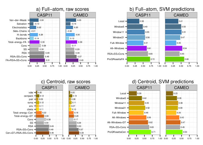
Figure 1: Spearman correlations of ProQRosFA and ProQRosCen input features with the target feature (S-score) without SVM training (raw scores) and after SVM training (SVM predictions). All the correlations are calculated on the local (residue) level. (A) Correlations of ProQRosFA input features with S-score. The terms in each group are summed up before we calculate the correlations. Negative correlations shown with positive bar lengths (only Solvation and Side-Chains correlations were negative). (B) Correlations of SVM predictions with S-score after training SVM on a subset of ProQRosFA input features. Local means all the energies are calculated over a single residue. Window5-11-21 means that all the energies are averaged over a window of 5-11-21 residues. Full-window means that all the energies are averaged over the whole model length. All-Windows includes all window sizes into the training. RSA, SS and Cons were used with the same window sizes as in ProQ2 when training SVM (see Methods) (C) Correlations of ProQRosCen input features with S-score. Global terms are only presented as a total energy, but not individual features. (D) Correlations of SVM predictions with S-score after training SVM on a subset of ProQRosCen input features. The window definitions are the same as in (B). Abbreviations: Total-energy-FA or FA—Total energy of full-atom energy terms, Total-energy-Cen or Cen—Total energy of centroid local energy terms, Total-energy-GT or GT—Total energy of centroid global energy terms, H-bonds—Hydrogen bonds, RSA—relative accessible surface area prediction agreement, SS—secondary structure prediction agreement, Cons—residue conservation. See Table 1 for a more detail explanation of the input features. Color scheme: shades of blue and purple—Rosetta full atom input features, shades of brown, yellow and orange—Rosetta centroid input features, shades of grey—sequence-dependent input features, shades of green—final predictors

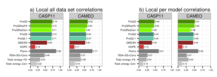
Figure 2: Spearman correlations of selected methods vs. S-score on local (residue) level. A) Correlations for the whole data set B) Average correlations for each model in the data set. ProQ2.1 is ProQ2 retrained on CASP9 data set with 30 models per target (the same training data set as ProQ3). RSA+SS+Cons is Relative Surface Area accessibility agreement plus Secondary Structure agreement plus Conservation without training (same as in Figure 1a and 1c). Total-energy-FA is the sum of Rosetta full-atom energy terms without training (same as in Figure 1a). Total-energy-Cen is the sum of Rosetta centroid energy terms without training (same as in Figure 1c). Color scheme: Shades of green—ProQ methods, shades of red—other single-model methods, shades of grey—reference methods.

Figure 3: Spearman correlations of selected methods vs. S-score on global (protein) level. A) Correlations for the whole data set B) Average correlations for each target in the data set. Color scheme and method definitions are the same as in Figure 2.

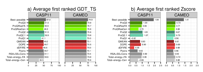
Figure 4: A) Average first ranked GDT_TS score for each method. Average is calculated over all targets in a data set. B) Average first ranked Z-score for each method. Z-score is defined as $(GDT\_TS_{first\_ranked}-mean(GDT\_TS))/standard\_deviation(GDT\_TS)$ where mean standard deviation (sd) is calculated for each target. Color scheme and method definitions are the same as in Figure 2.

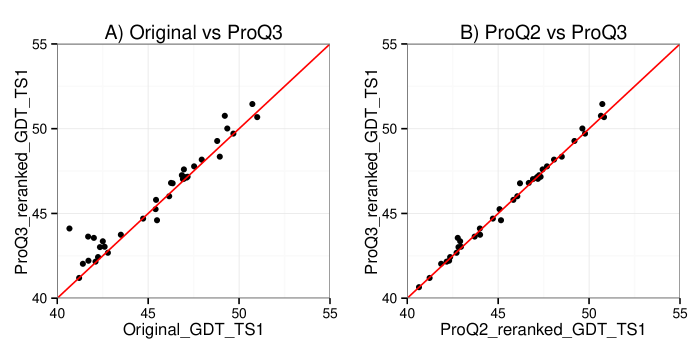
Figure 5: A) Original vs. ProQ3-reranked average GDT_TS1 scores for each method B) Original vs. ProQ3-reranked average GDT_TS1 scores for each method. Only methods with average first ranked GDT_TS greater than 40 are shown (36 out of 44 methods).

Our aim of the project was to improve ProQ2 method, which is already one of the best, if not the best, single-model methods for model quality assessment. ProQ2 is a machine learning based method that is based on Support Vector Machines (SVM) that was recently implemented as a scoring function in Rosetta [16]. It has a variety of input features, including atom-atom contacts, residue-residue contacts, surface area accessibilities, secondary structure and residue conservation.

When developing a new predictor we were looking for new input features that we could use and decided to use Rosetta energy functions. Rosetta has two types of energy functions: one that uses an all-atom protein model (“full-atom” model) and the other one that uses only a protein backbone (“centroid” model). In general, the type of function that uses an all-atom model gives more accurate results, but the other type can be useful when an all-atom model is not available. Therefore, we developed two new predictors: one that uses all-atom model (“ProQRosFA”) and one that uses only the protein backbone (“ProQRosCen”). In addition, we have developed a third predictor that combines ProQRosFA, ProQRosCen and ProQ2 (“ProQ3”).

The new predictors still use SVMs. They also inherit the sequence-dependent features from ProQ2—relative surface area accessibility agreement, secondary structure agreement and residue conservation. All other input features in ProQRosFA and ProQRosCen are Rosetta energy terms. Below we describe the new predictors in more detail.

2.1 ProQRosFA input features

Table 1: The description of features used in ProQRosFA and ProQRosCen predictors.

Feature	Predictor	Description
Van-der-Waals	ProQRosFA	A sum of fa_atr, fa_rep and fa_intra_rep energy terms in Rosetta
Solvation	ProQRosFA	fa_sol energy term in Rosetta
Electrostatics	ProQRosFA	fa_elec energy term in Rosetta
Side-chains	ProQRosFA	pro_close, dslf_fa13, fa_dun and ref energy terms in Rosetta
Hydrogen bond	ProQRosFA	hbond_sr_bb, hbond_lr_bb, hbond_bb_sc and hbond_sc energy terms in Rosetta
Backbone	ProQRosFA	rama, omega and p_aa_pp energy terms in Rosetta
Total-energy-FA	ProQRosFA	A weighted sum of all energy terms used in ProQRosFA predictor. The weights are the same as in “Talaris2013”.
vdw	ProQRosCen	vdw energy term in Rosetta.
cenpack	ProQRosCen	cenpack energy term in Rosetta.
pair	ProQRosCen	pair energy term in Rosetta.
rama	ProQRosCen	rama energy term in Rosetta.
env	ProQRosCen	env energy term in Rosetta.
cbeta	ProQRosCen	cbeta energy term in Rosetta.
Total-energy-Cen	ProQRosCen	A sum of all local energy terms used in ProQRosCen predictor: vdw, cenpack, pair, rama, env, cbeta. All weights in a sum are equal to one.
Total-energy-GT	ProQRosCen	A sum of all global energy terms used in ProQRosCen predictor: rg, hs_pair, ss_pair, sheet, rsigma, co. All weights in a sum are equal to one.
RSA	All predictors	Relative surface area accessibility agreement between the model and the prediction from the sequence.
SS	All predictors	Secondary structure agreement between the model and the prediction from the sequence.
Cons	All predictors	Residue conservation in the sequence

Table 2: Average GDT_TS1 for each method before and after reranking

Method	Original GDT_TS1	ProQ3 GDT_TS1	ProQ2 GDT_TS1	Optimal GDT_TS1
QUARK	51.0	50.7	50.8	53.2
Zhang-Server	50.7	51.5	50.7	53.4
nns	49.7	49.7	49.8	51.7
myprotein-me	49.4	50.0	49.6	52.6
BAKER-ROSETTASERVER	49.2	50.8	50.7	53.2

For ProQRosFA predictor we used “Talaris 2013” that is currently the default score function in Rosetta. This score function consists of 16 terms and the “Total energy” term. A SVM model was trained using all of these energy terms as input features. However, before we analyse the final performance of ProQRosFA predictor we would like to show how well the input features were correlated with our target function (S-score) without training. A stronger correlation between input feature and the target function is more useful for the final predictor.

Since there are many individual input features (17), rather than showing the correlation for each separate feature, we will group the features into 7 groups and show the correlations for each group: Van-der-Waals, Solvation, Electrostatics, Side-Chains, Hydrogen bond, Backbone and Total-energy-FA. Note that even though we group features here for visualising their performance, they were all used separately when training SVM.

Figure 1a shows Spearman correlations against our target function (S-score) for each of the 7 groups. On both data sets, the correlations for Electrostatics, Van-der-Waals and Hydrogen bond and Total-energy-FA groups were higher than Solvation, Side-Chains and Backbone. The Total-energy-FA group includes the features from all other groups so it has the highest correlation, as expected. However, the difference in correlations between Van-der-Waals and Total-energy-FA groups is small.

Relative surface area accessibility agreement (RSA) and secondary structure agreement (SS) have higher correlation on the CASP11 than on the CAMEO data set. This maybe due to the fact that models in CAMEO are higher quality than in CASP11 data set (see Table 3). High quality models usually have good RSA and SS agreements and, therefore, these features are not as useful as for lower quality models. Residue conservation (Cons) also has higher correlation on CASP11 data set and the difference here is even larger. This is probably because CAMEO targets are more conserved and are easier to model.

After adding sequence-dependent features (RSA, SS, Cons) to the Total-energy-FA of Rosetta energies the correlation increases on both CASP11 and CAMEO data sets even without training. This result is interesting because it shows that the Rosetta energy potentials could be improved by sequence-dependent features. However, on CASP11 RSA has almost as high correlation (0.49) as the combined term FA+RSA+SS+Cons (0.51), which suggest that RSA alone is a strong feature. In fact, it is so strong that adding SS and Cons (RSA+SS+Cons) even makes the correlation slightly smaller than RSA alone.

The correlations can be improved by training SVMs with input features averaged over a sequence window (see Figure 1b). We tried several different window sizes and observed that on CASP11 the highest correlation (0.56) was obtained for window of size 21, while on CAMEO the highest correlation was obtained for window of size 11 (0.51). If all different window sizes are combined, the correlation increases up to 0.61 on CASP11 and up to 0.54 on CAMEO data sets. It is interesting that on CASP11 data set sequence-dependent features alone have a higher correlation than all the Rosetta features with all window sizes combined (0.65 vs 0.61). This does not hold for CAMEO data set where Rosetta features have higher correlation than the sequence-dependent features (0.54 vs 0.45). However, when Rosetta features with sequence-dependent features are combined, the correlation increases on both of the data sets (0.72 and 0.60 on CASP11 and CAMEO respectively).

2.2 ProQRosCen input features

Centroid scoring functions have an advantage that they can be used even if the exact position of side chains in the model is not known. It is also less sensitive to exact atomic positions making it possible to score models from different methods with a lower risk of high repulsive score from steric clashes.

The standard centroid scoring function in Rosetta is called “cen_std” and it includes four local centroid energy terms: vdw, pair, env, cbeta. However, it does not include a couple of other local centroid energy terms (cenpack and rama). Therefore, we have defined our own scoring function that includes all energy terms in “cen_std” plus these two additional ones.

On both CASP11 and CAMEO data sets the two additional energy terms (cenpack and rama) have the highest correlation among all local energy terms, except the Total-energy-Cen term. The lowest correlation on both data sets is for vdw energy term (Figure 1c).

The standard scoring functions in Rosetta “Talaris2013” and “cen_std” include only the local energy terms meaning that these energy terms are defined for each separate residue in the protein. However, in Rosetta there are also global energy terms that are only defined for the whole protein model. Most of these global energy terms are centroid. We have included 6 global centroid energy terms to our ProQRosCen predictor: rg, hs_pair, ss_pair, sheet, rsigma, co. Figure 1c shows the correlation between the target function and the Total-energy-Cen of these global terms (Total-energy-GT). Note that ProQRosCen predictor includes the same sequence-dependent features as in ProQRosFA. Therefore, the correlations for sequence-dependent features in Figure 1c and Figure 1a are the same.

Similarly to what we saw for ProQRosFA, the correlation for the combined term Cen+GT+RSA+SS+Cons is higher than the correlation for Total-energy-Cen or Total-energy-GT alone. However, on CASP11 data set the correlation for RSA is as high as the correlation for the combined term Cen+GT+RSA+SS+Cons (0.49), which once again confirms that RSA is a very strong feature.

Just like for ProQRosFA the correlation can be improved by training SVMs with input features averaged over a sequence window (see Figure 1d). On CASP11 data set the highest correlation is again for window of size 21 (0.52) and on CAMEO data set the highest correlation is for window of size 11 (0.39). Combining all window sizes improves the correlation up to 0.56 on CASP11 and up to 0.43 on CAMEO. Since global energy terms are only defined for the whole protein, they cannot be averaged over different window sizes. All-Windows variable in Figure 1d includes only local energy terms. When local energy terms averaged over different window sizes (All-Windows) are combined with global energy terms (GT), the correlation further increases to 0.62 on CASP11 and 0.47 on CAMEO. After adding sequence-dependent features (RSA+SS+Cons), the correlation of the final centroid predictor reaches 0.71 on CASP11 and 0.53 on CAMEO.

2.3 ProQ3

ProQ3 combines the three predictors: ProQ2, ProQRosFA and ProQRosCen. All the features from three predictors are put together with the sequence-dependent features that are common to all three (RSA, SS, Cons) into a new SVM that predicts the score.

2.4 Benchmark

In the following sections we will compare ProQ2, ProQRosFA, ProQRosCen and ProQ3 results with other single-model methods: QMEAN [17], DOPE [18], DDFIRE [19], ProQ1 [4]. Only single-model methods that have publicly available stand-alone versions were included. Two versions of ProQ2 are included—the original one and one that was retrained on CASP9 dataset with 30 models per target (the same training data set as ProQ3). There is also one consensus method included for a reference—Pcons [6]. Finally, sequence-dependent features and Rosetta total energies are included as a reference.

We will compare the method performance in three categories: local (residue) level correlations, global (protein) level correlations and model selection. Two methods (dDFire and ProQ1) provide only the global level predictions, so they were not included into the local level evaluation category.

2.4.1 Local correlations

All of our new predictors (ProQRosFA, ProQRosCen and ProQ3) are trained on the local level. In other words, every residue in the protein model is assigned training feature values and a target value (S-score). Therefore, it makes sense to look at how well do our predictions correlate with the target value on the local (residue) level first.

We have evaluated all methods in two ways: by calculating the correlation for all data set (Figure 2a) and by calculating the average correlation for each protein model in the data set (Figure 2b). The first evaluation shows how well methods separate between well-modeled and badly-modeled residues in general while the second evaluation shows how well methods separate well-modeled and badly-modeled residues inside a particular model.

ProQ3 outperforms all other single-model methods on both data sets and in both evaluations. The largest improvement over the original ProQ2 is on CAMEO all data set correlation (0.62 vs. 0.56). ProQRosFA performs equally or slightly better than the original ProQ2. ProQRosCen performs slightly worse, but still on par with QMEAN. Both QMEAN and DOPE perform equally or worse than any ProQ method with the only exception of QMEAN having a higher per model correlation than ProQRosCen on CAMEO data set (0.46 vs. 0.38, Figure 2b). The reference consensus method (Pcons) outperforms all other methods as expected. However, improving single-model methods is still important for the reasons that were mentioned in the introduction. The sequence-dependent features (RSA+SS+Cons) and Rosetta total energies (Total-energy-FA and Total-energy-Cen) perform far worse than ProQRosFA and ProQRosCen. Thus, there is a lot to be gained by using any of any of the methods developed here.

All differences in local all data set correlations (Figure 2a) are significant with P-values ¡ $10^{-3}$ according to Fisher r-to-z transformation test. All differences in mean per-model correlations were significant with P-values ¡ $10^{-3}$ according to Wilcoxon signed-rank test.

2.4.2 Global correlations

Even though ProQRosFA, ProQRosCen and ProQ3 are trained on the local level, they also provide global predictions of a model quality. The global predictions are derived from the local predictions, by summing up all local predictions for a protein model and dividing the sum by the model length. The target function (S-score) is also local by its nature, but can be turned to global in exactly the same way.

We have evaluated all methods again in two ways: by calculating the correlation for all data set (Figure 3a) and by calculating the average correlation for each target in the data set (Figure 3b). The first evaluation shows how well a method separates good and bad models in general while the second evaluation shows how well a method separates good and bad models for the same target.

ProQ3 again outperforms all other single-model methods on both data sets and in both evaluations. The largest improvement over the original ProQ2 is in CAMEO all data set correlation (0.74 vs. 0.69), Figure 3a. Both ProQRosFA and ProQRosCen performance is close to ProQ2 but better than QMEAN. Like in the local case, the reference consensus method (Pcons) outperforms all other methods in most of the evaluations. However, ProQ3 performs better than Pcons on per target correlations on CAMEO data set (0.53 vs. 0.51), Figure 3b. This shows that consensus methods do not perform very well on per-target correlations when the number of models for a target is small (the average number of models per target on CAMEO data set is only 30, see Table 3). Sequence-dependent features (RSA+SS+Cons) and raw Rosetta energies (Total-energy-FA and Total-energy-Cen) again perform worse than ProQRosFA and ProQRosCen. However, it is interesting to notice that these measures often perform better than dDFIRE, DOPE and in some cases even QMEAN.

All differences in global all data set correlations (Figure 3a) are significant with P-values ¡ $10^{-3}$ according to Fisher r-to-z transformation test. The number of targets was too small to get significant differences in per-target correlation means according to Wilcoxon signed-rank test.

2.4.3 Model selection

An important task of model quality assessment program (MQAP) is to be able to find the best protein model among several possible ones. We have evaluated MQAP performance in this task by calculating the average of first ranked GDT_TS scores (GDT_TS1) and the average of first ranked Z-scores for each method (see Figure 4).

Interestingly, the retrained version of ProQ2 (ProQ2.1) performs better than ProQ3 both in terms of the average first ranked GDT_TS score and Z-scores. Both ProQ2 and ProQ3 outperform all other methods including Pcons. As shown already at CASP8 [20], consensus methods are not performing optimal in model selection and this is one of the major reasons why we need to develop single-model methods.

After analyzing possible reasons for the better performance of ProQ2 over ProQ3 in model selection, we have found out that ProQ3 is extremely biased towards selecting Robetta [21] models. In CASP11, ProQ3 selects Robetta models 65 out of 83 times and in CAMEO 609 out of 676 times. For comparison, ProQ2 selects Robetta models 23 times in CASP11 and 444 times in CAMEO. The reason why ProQ3 selects Robetta models so often is most likely because Robetta server models are already optimized using the Rosetta energy function. Since ProQ3 also uses Rosetta energy terms as input features, it is not a big surprise that it overestimates quality of Robetta models. However, this does not harm ProQ3 performance too much, because Robetta models are often of high quality. Demonstrated by the fact that 20 targets in CASP11 and 336 targets in CAMEO Robetta models are the best possible choice. Still, ProQ3 bias towards Robetta models makes it perform slightly worse than ProQ2 in model selection.

2.4.4 Using ProQ3 to rerank models in structure prediction

In CASP experiment, structure prediction groups have to submit 5 models for each target and rank them from best to worst. In CASP11 Kryshtafovych et al. drew attention that some of the structure prediction groups could benefit from using ProQ2 when ranking the models of their method [9]. Similarly to their analysis, we evaluated how the average GDT_TS of the first ranked models would have changed for each group if the structure prediction groups had been using ProQ2 or ProQ3.

Figure 5a shows the average first ranked GDT_TS scores for each method before and after reranking them with ProQ3. We can see that most of the methods (26 out of 36) would have benefited from using ProQ3 when ranking their models. Only for 8 methods the score would have gotten worse and for 2 methods it would have stayed the same.

Figure 5a also suggests a ranking of the structure prediction groups based on the average first ranked GDT_TS. If we take all points from right to left we will get the original ranking of the groups and if we take the points from top to bottom, we will get the ranking of the groups if all of them were using ProQ3 to pick the best model out of five. We can see that the ranking would change for many of the structure prediction groups. In fact, the ranking would significantly change even for the best structure prediction groups, as it is shown in Table 2. If Zhang-Server was using ProQ3, it would be in the first place instead of second and if BAKER-ROSETTASERVER was using ProQ3, it would be in the second place instead of fifth. That clearly shows the benefit of developing good model quality assessment methods.

Figure 5b compares ProQ2 and ProQ3 performance in ranking the models for each structure prediction group. We can see that more than half of the groups (19 out of 36) would have benefited more from using ProQ3 than from using ProQ2. 15 out of 36 groups would have benefited more from using ProQ2 than ProQ3 and for 2 groups there would be no difference.

It is interesting to notice that even BAKER-ROSETTASERVER (Robetta method) group would have benefited more from using ProQ3 than ProQ2. It seems that when models from the same method are evaluated, ProQ3 tendency to overestimate the quality of Rosetta models does not matter. Since all models come from the same method, the bias cancels out and the ranking of the models within the group stays accurate.

3 Methods

3.1 Training and test data sets

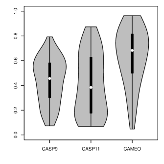
Figure 6: Violin plot of the distribution of mean model quality per target on CASP9, CASP11 and CAMEO data sets.

Table 3: Training and test data sets.

	CASP9	CASP9 random subset	CASP11	CAMEO
Number of targets	117	117	83	676
Total number of models	33440	3505	15334	20206
Total number of residues	6757370	712751	3665828	5027933
Average number of models per target	286	30	185	30
Average number of residues in a model	202	203	239	249
Mean model quality	0.44	0.44	0.40	0.64
Mean standard deviation of model quality (per target)	0.14	0.14	0.12	0.09

The original ProQ2 was trained on CASP7 data set with 10 models per target selected at random. We have noticed that the performance slightly increases when ProQ2 is retrained on CASP9 data set with 30 models per target selected at random (see Figure 2 and 3). Therefore, we have used the latter as the training data set for ProQRosFA, ProQRosCen and ProQ3.

Two data sets were used for testing: CASP11 and CAMEO. Only server models were used in CASP11 data set. All CAMEO models from 1 year time period were used (2014-06-06–2015-05-30). Targets that were shorted than 50 residues were filtered out both from CASP11 and CAMEO data sets. CASP9 data set did not have such short targets.

Table 3 shows statistics on the data set sizes and model quality. We can see from the table that CASP9 and CASP11 data set has more models per target, but CAMEO data set has more targets. These two facts turn out to compensate each other and the final number of models is in the same range on all data sets.

Mean model quality on CASP9 and CASP11 data sets is similar (0.44 and 0.40), but on CAMEO data set it is considerably higher (0.64). Mean standard deviation of model quality (calculated per-target) on CAMEO data set is the smallest (0.09).

Figure 6 shows the distribution of mean model quality on CASP9, CASP11 and CAMEO data sets. Mean model quality for most of the targets is clustered around 0.6 on CASP9 data set, around 0.8 on CAMEO data set. CASP11 has more models of bad quality than the other data sets with a small peak around 0.2.

3.2 Side chain re-sampling and energy minimization

Protein models can be generated by different methods that employ different modeling strategies resulting in similar models but vastly different Rosetta energy terms. For instance, some of models in our data sets had very large repulsive energy terms (fa_rep) because of steric clashes. To account for model generation differences, the side-chains of all models were rebuild using the backbone-dependent rotamer library in Rosetta. This was followed by a short backbone restrained energy minimization protocol using the Rosetta energy function. This ensured that the Rosetta energy terms for the models were at their minimium values.

The side-chains were rebuilt with a backbone-dependent rotamer library implemented in the repack protocol. 10 different decoys were generated for each model and the best one was selected based on ProQ2 score.

Some of the protein models in our data sets had very large Lennard-Jones repulsive energy terms (fa_rep). To account for this we have run a short energy minimization protocol (-ddg:min_cst). This has moved protein models from the local maxima of energies without moving the backbones.

3.3 Implementation

We have used per_residue_energies binary in Rosetta (2014 week 5 release) to get per residue energies for local full-atom and centroid energy terms. talaris2013.wts weight file was used for local full-atom scoring function. For local centroid scoring function we have defined a custom weight file that included vdw, cenpack, pair, rama, env, cbeta energy terms with all weights equal to one.

For global centroid scoring function, Rosetta score binary was used. A custom weight file included rg, hs_pair, ss_pair, sheet, rsigma, co energy terms with all weights equal to one.

SVM predictor works best when the input features are either scaled between -1 and 1 or between 0 and 1 [22]. This is usually achieved by linear scaling of the input features. However, in order to avoid outliers we decided to use a sigmoidal function ($1/(1+e^{x})$) to scale all of the terms between 0 and 1.

After sigmoidal transformation, all of the local full-atom and centroid energy terms were averaged using window sizes of 5, 11 and 21 residues. Additionally, the local (single-residue) and the full-window (averaged over the whole protein) energy terms were added to the training.

Global centroid energy terms are defined for the whole protein, so they cannot be averaged using different window sizes. On the other hand, they depend on the protein size, so they need to be normalized. rg term depends on the protein size L by a factor of $L^{0.4}$ [23] by which it was normalized. After performing a linear regression on the logarithmic scale we found that co depends on the protein size by $L^{0.72}$ and the other terms by L, so they were normalized accordingly.

3.4 Target function

We have used the same target function as in ProQ2, the S-score. S-score is defined as:

$$S_{i}={1\over{1+(d_{i}/d_{0})^{2}}}$$ (1)

where $d_{i}$ is the distance for residue i between the native structure and the model in the superposition that maximizes the sum of $S_{i}$ and $d_{0}$ is a distance threshold. The distance threshold was set to 3Å, as in the original version of ProQ2.

3.5 Sequence-dependent features

The sequence-dependent features, RSA, SS and Cons (see Table 1) were implemented the same way as in ProQ2. Sequence profiles were derived using three iterations of PSI-BLAST v.2.2.26 [24] against Uniref90 (downloaded 2015-10-02) [25] with a $10^{-3}$ E-value inclusion threshold. Secondary structure of the protein was calculated from the model using STRIDE [26] and predicted from the sequence using PSIPRED [27]. The agreement between the prediction and the actual secondary structure in the model was calculated over the window of 21 residues and over the full-window over the whole protein. Also, the probability of having a particular secondary structure type in every single position was calculated. Relative surface area accessibility was calculated by NACCESS [28] and predicted from the sequence by ACCpro [29]. The RSA agreement was also calculated over the window of 21 residues and over the full-window over the whole protein. The actual secondary structure and relative surface area was not added to ProQRosFA and ProQRosCen predictors, only the agreement scores. For residue conservation “information per position” scores were extracted from PSI-BLAST matrix with window size of 3 residues.

3.6 SVM training

A linear SVM model was trained using $SVM^{ligth}$ package V6.02 [30]. All parameters were kept at their default values.

3.7 Other tools

R zoo package [31] was used to average values over varying window sizes. needle program from EMBOSS package [32] was used to align model and target sequences.

4 Conclusion

Here, we present ProQ3, a novel protein quality prediction program. ProQ3 is based on a combination of three predictors, ProQ2, ProQCenFA and ProQRosFA. All these three predictors are trained in a similar way but the way the inputs are presented for them is different. The performance of each individual predictors is similar and the combination is superior to any of the three individual predictors.

Funding

This work was supported by grants from the Swedish Research Council (VR-NT 2012-5046 to AE and 2012-5270 to BW). Computational resources at the National Supercomputing Center were provided by SNIC.

References

- [1] M. Hendlich, P. Lackner, S. Weitckus, H. Floeckner, R. Froschauer, K. Gottsbacher, G. Casari, and M. Sippl. Identification of native protein folds amongst a large number of incorrect models. the calculation of low energy conformations from potentials of mean force. J Mol Biol, 216(1):167–180, Nov 1990.
- [2] D. Jones, W. Taylor, and J. Thornton. A new approach to protein fold recognition. Nature, 358(6381):86–89, Jul 1992.
- [3] R. Luthy, J. Bowie, and D. Eisenberg. Assessment of protein models with three-dimensional profiles. Nature, 356(6364):83–85, Mar 1992.
- [4] B. Wallner and A. Elofsson. Can correct protein models be identified? Protein Sci, 12(5):1073–1086, May 2003.
- [5] C. Colovos and T. Yeates. Verification of protein structures: patterns of nonbonded atomic interactions. Protein Sci, 2(9):1511–1519, Sep 1993.
- [6] B. Wallner and A. Elofsson. Identification of correct regions in protein models using structural, alignment, and consensus information. Protein Sci, 15(4):900–913, Apr 2006.
- [7] B. Wallner, H. Fang, and A. Elofsson. Automatic consensus-based fold recognition using pcons, proq, and pmodeller. Proteins, 53 Suppl 6:534–541, 2003.
- [8] A. Ray, E. Lindahl, and B. Wallner. Improved model quality assessment using proq2. BMC Bioinformatics, 13:224, 2012.
- [9] A. Kryshtafovych, A. Barbato, B. Monastyrskyy, K. Fidelis, T. Schwede, and A. Tramontano. Methods of model accuracy estimation can help selecting the best models from decoy sets: Assessment of model accuracy estimations in CASP11. Proteins, Sep 2015.
- [10] J. Lundstrom, L. Rychlewski, J. Bujnicki, and A. Elofsson. Pcons: a neural-network-based consensus predictor that improves fold recognition. Protein Sci, 10(11):2354–2362, Nov 2001.
- [11] K. Ginalski, A. Elofsson, D. Fischer, and L. Rychlewski. 3d-jury: a simple approach to improve protein structure predictions. Bioinformatics, 19(8):1015–1018, May 2003.
- [12] B. Wallner and A. Elofsson. Pcons5: combining consensus, structural evaluation and fold recognition scores. Bioinformatics, 21(23):4248–4254, Dec 2005.
- [13] B. Wallner and A. Elofsson. Prediction of global and local model quality in CASP7 using pcons and proq. Proteins, 69 Suppl 8:184–193, 2007.
- [14] C. Pettitt, L. McGuffin, and D. Jones. Improving sequence-based fold recognition by using 3d model quality assessment. Bioinformatics, 21(17):3509–3515, Sep 2005.
- [15] S. Ovchinnikov, D. Kim, R. Wang, Y. Liu, F. DiMaio, and D. Baker. Improved de novo structure prediction in CASP11 by incorporating co-evolution information into rosetta. Proteins, Dec 2015.
- [16] K. Uziela and B. Wallner. Proq2: Estimation of model accuracy implemented in rosetta. Bioinformatics, Jan 2016.
- [17] P. Benkert, S. Tosatto, and D. Schomburg. QMEAN: A comprehensive scoring function for model quality assessment. Proteins, 71(1):261–277, Apr 2008.
- [18] M. Shen and A. Sali. Statistical potential for assessment and prediction of protein structures. Protein Sci, 15(11):2507–2524, Nov 2006.
- [19] Y. Yang and Y. Zhou. Specific interactions for ab initio folding of protein terminal regions with secondary structures. Proteins, 72(2):793–803, Aug 2008.
- [20] P. Larsson, M. Skwark, B. Wallner, and A. Elofsson. Assessment of global and local model quality in CASP8 using pcons and proq. Proteins, 77 Suppl 9:167–172, 2009.
- [21] K. Simons, C. Kooperberg, E. Huang, and D. Baker. Assembly of protein tertiary structures from fragments with similar local sequences using simulated annealing and bayesian scoring functions. J Mol Biol, 268(1):209–225, Apr 1997.
- [22] C. Hsu, C. Chang, and C. Lin. A practical guide to support vector classification, 2010.
- [23] D. Neves and R. Scott, 3rd. Monte carlo calculations on polypeptide chains. VIII. distribution functions for the end-to-end distance and radius of gyration for hard-sphere models of randomly coiling poly(glycine) and poly(l-alanine). Macromolecules, 8(3):267–271, May 1975.
- [24] S. Altschul, T. Madden, A. Schaffer, J. Zhang, Z. Zhang, W. Miller, and D. Lipman. Gapped BLAST and PSI-BLAST: a new generation of protein database search programs. Nucleic Acids Res, 25(17):3389–3402, Sep 1997.
- [25] B. Suzek, H. Huang, P. McGarvey, R. Mazumder, and C. Wu. Uniref: comprehensive and non-redundant uniprot reference clusters. Bioinformatics, 23(10):1282–1288, May 2007.
- [26] D. Frishman and P. Argos. Knowledge-based protein secondary structure assignment. Proteins, 23(4):566–579, Dec 1995.
- [27] D. Jones. Protein secondary structure prediction based on position-specific scoring matrices. J Mol Biol, 292(2):195–202, Sep 1999.
- [28] S. J. Hubbard and J. M. Thornton. ’NACCESS’, computer program. Technical report, Department of Biochemistry Molecular Biology, University College London, 1993.
- [29] J. Cheng, A. Randall, M. Sweredoski, and P. Baldi. SCRATCH: a protein structure and structural feature prediction server. Nucleic Acids Res, 33(Web Server issue):W72–6, Jul 2005.
- [30] T. Joachims. Learning to classify text using support vector machines: Methods, theory and algorithms. Kluwer Academic Publishers, 2002.
- [31] A. Zeileis and G. Grothendieck. zoo: S3 infrastructure for regular and irregular time series. Journal of Statistical Software, 14(6):1–27, 2005.
- [32] P. Rice, I. Longden, and A. Bleasby. EMBOSS: the european molecular biology open software suite. Trends Genet, 16(6):276–277, Jun 2000.