Particle-like wave packets in complex scattering systems

Abstract

A wave packet undergoes a strong spatial and temporal dispersion while propagating through a complex medium. This wave scattering is often seen as a nightmare in wave physics whether it be for focusing, imaging or communication purposes. Controlling wave propagation through complex systems is thus of fundamental interest in many areas, ranging from optics or acoustics to medical imaging or telecommunications. Here, we study the propagation of elastic waves in a cavity and a disordered waveguide by means of laser interferometry. From the direct experimental access to the time-delay matrix of these systems, we demonstrate the existence of particle-like wave packets that remain focused in time and space throughout their complex trajectory. Due to their limited dispersion, their selective excitation will be crucially relevant for all applications involving selective wave focusing and efficient information transfer through complex media.

I Introduction

Waves propagating in complex media typically undergo diffraction and multiple scattering at all the inhomogeneities they encounter. As a consequence, a wave packet suffers from strong temporal and spatial dispersion while propagating through a scattering medium. Eventually, the incident wave is converted into a diffuse halo that gives rise to a complicated interference pattern (speckle) at the output of the medium. Albeit complex, this wave-field remains, however, deterministic. By actively shaping the wave-field at the input, one can manipulate the interference between all the scattering paths that the wave can follow. On the one hand, this insight has given rise to spectacular focusing schemes in which scattering enables - rather than impedes - wave focusing and pulse compression Derode et al. (1995); Tanter et al. (2000); Lerosey et al. (2004, 2007); Vellekoop and Mosk (2007); Popoff et al. (2010); Aulbach et al. (2011); McCabe et al. (2011); Katz et al. (2011). On the other hand, it can lead to an optimized control of wave transport Vellekoop and Mosk (2008); Pendry (2008); Kim et al. (2012); Shi and Genack (2012). A designed wave-front can, e.g., be completely transmitted/reflected at will Choi et al. (2011); Gérardin et al. (2014) as a result of a multiple scattering interference that is intrinsically narrowband Hsu et al. (2015). Here we will aim at the more challenging goal to generate states that are fully transmitted/reflected, yet very robust in a broadband spectral range. As we will demonstrate explicitly, this goal can be reached by way of highly collimated scattering states that are concentrated along individual particle-like bouncing patterns inside the medium Rotter et al. (2011). By avoiding the multi-path interference associated with conventional scattering states, these wave beams also avoid the frequency sensitivity associated with this interference. As we shall see, particle-like scattering states give rise, in the time domain, to wave packets that remain focused in time and space throughout their trajectory within the medium. This crucial feature makes these states uniquely suited for many applications in a variety of fields, ranging from high intensity focused ultrasound Aubry et al. (2008); Cochard et al. (2009) or underwater acoustics Edelmann et al. (2002); Prada et al. (2007) to endoscopic microscopy Cizmar and Dholakia (2012); Papadopoulos et al. (2012); Plöschner et al. (2015), fibre optics Fan and Kahn (2005); Juarez et al. (2012); Carpenter et al. (2015); Xiong et al. (2016); Carpenter and Wilkinson (2012) or telecommunications Salz (1985); Raleigh and Cioffi (1998); Tulino and Verdù (2004).

The key aspect of our experimental study is to demonstrate that these particle-like wave packets can be created just based on the information stored in the scattering matrix Rotter et al. (2011). This highly dimension $\mathbf{S}$-matrix relates any arbitrary wave-field at the input to the output of the scattering medium, and in principle, allows the reconstruction or prediction of either. It fully describes wave propagation across a scattering medium and can meanwhile be routinely measured not only in acoustics Sprik et al. (2008); Aubry and Derode (2009), but also in microwave technology Shi and Genack (2012); Dietz et al. (2012) and optics Popoff et al. (2010); Kim et al. (2012). The sub-blocks of the scattering matrix contain the complex-valued transmission ($\mathbf{t},\mathbf{t^{\prime}}$) and reflection ($\mathbf{r}$, $\mathbf{r^{\prime}}$) matrices with a certain number $N$ of input and output channels,

$$\mathbf{S}=\left(\begin{array}[]{cc}\mathbf{r}&\mathbf{t^{\prime}}\\ \mathbf{t}&\mathbf{r^{\prime}}\end{array}\right).$$ (1)

To describe the statistical properties of $\mathbf{S}$ for wave transport through complex media, random matrix theory (RMT) has been very successful Beenakker (1997). One of the striking result of RMT is the universal bimodal distribution followed by the transmission eigenvalues $T$ of $\mathbf{tt^{{\dagger}}}$ footnote1 through diffusive media Beenakker (1997); Dorokhov (1984); Imry (1986) or chaotic cavities Baranger and Mello (1994); Jalabert et al. (1994). In contradiction with a classical diffusion or chaotic picture, a substantial fraction of propagation channels are found to be essentially closed ($T\sim 0$) or open ($T\sim 1$). Going beyond such a statistical approach, Rotter et al. Rotter et al. (2011) recently showed how a system-specific combination of fully open or fully closed channels may lead to scattering states that follow the particle-like bouncing pattern of a classical trajectory throughout the entire scattering process. Such particle-like scattering states with transmission close to 1 or 0 are eigenstates of the Wigner-Smith time-delay matrix:

$$\mathbf{Q}=-\frac{i}{2\pi}\mathbf{S}^{{\dagger}}\partial_{f}\mathbf{S},$$ (2)

where $\partial_{f}$ denotes the derivative with respect to the frequency $f$. Originally introduced by Wigner in nuclear scattering theory Wigner (1955) and extended by Smith to multichannel scattering problems Smith (1960), the $\mathbf{Q}$-matrix generally describes the time that the incoming wave accumulates due to the scattering process: each eigenvalue yields the time delay of the associated scattering state. Compared to a mere study of the $\mathbf{S}$-matrix, the $\mathbf{Q}$-matrix provides an elegant and powerful tool to harness the dispersion properties of a complex medium. In this article, we show, in particular, how a time-delay eigenstate can be engineered to be “particle-like” not only in its stationary wave function patterns Rotter et al. (2011), but also in the sense that a non-dispersive wave packet can be propagated along the corresponding particle-like bouncing pattern. The associated eigenvalue of $\mathbf{Q}$ then corresponds to the propagation-time of this wave packet.

Our experimental setup consists of an elastic cavity and a disordered elastic wave guide at ultrasound frequencies [see Fig. 1]. In a first step we measure the entries of the $\mathbf{S}$- and $\mathbf{Q}$-matrices over a large bandwidth using laser-ultrasonic techniques. The eigenvalues of the transmission matrix are shown to follow the expected bimodal distributions in both configurations. The wave-fields associated with the open/closed channels are monitored within each system in the time domain by laser interferometry. Not surprisingly, they are shown to be strongly dispersive as they combine various path trajectories and thus many interfering scattering phases. To reduce this dispersion and to lift the degeneracy among the open/closed channels, we consider the eigenstates of the $\mathbf{Q}$-matrix that have a well-defined time-delay, corresponding to a wave that follows a single path trajectory. In transmission, a one-to-one association is found between time-delay eigenstates and ray-path trajectories. The corresponding wave functions are imaged in the time domain by laser interferometry. The synthesized wave packets are shown to follow particle-like trajectories along which the temporal spreading of the incident pulse is minimal. In reflection, the $\mathbf{Q}$-matrix yields the collimated wave-fronts that focus selectively on each scatterer of a multi-target medium. Contrary to alternative approaches based on time-reversal techniques Prada and Fink (1994); Prada et al. (1996); Popoff et al. (2011); Badon et al. (2015), the discrimination between several targets is not based on their reflectivity but on their position. The eigenvalues of $\mathbf{Q}$ directly yield the time-of-flight of the pulsed echoes reflected by each scatterer.

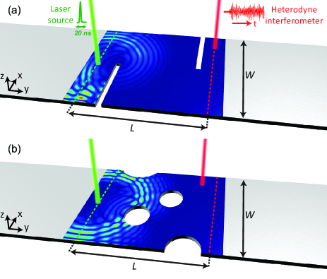
Figure 1: The two systems under investigation consist (a) of a regular cavity and (b) of a disordered slab machined in an elastic plate. In both configurations, the $\mathbf{S}$-matrix is measured in the time-domain between two arrays of points placed on the left and right sides of the system (see Appendix A). Flexural waves are generated on each point by a pulsed laser via thermo-elastic conversion over a focal spot of 1 mm². The normal component of the plate vibration is measured with an interferometric optical probe. The laser source and the probe are both mounted on 2D translation stages.

II Experimental results

II.1 Revealing the open and closed channels in a cavity

The waves we excite and measure are flexural waves in a duralumin plate of dimension $500\times 40\times 0.5\text{\,}\mathrm{m}\cubicmetre$ [see Fig. 1].The frequency range of interest spans from $0.23\text{\,}\mathrm{t}$o $0.37\text{\,}\mathrm{MHz}$ ($\Delta f=0.14$ MHz) with a corresponding average wavelength $\lambda$ of $3.5\text{\,}\mathrm{mm}$. We thus have access to $N=2W/\lambda\sim 22$ independent channels, $W$ being the width of the elastic plate. Two complex scattering systems are built from the homogeneous plate: (i) a regular cavity formed by cutting the plate over $20\text{\,}\mathrm{mm}$ on both sides of the plate [see Fig. 1(a)] and (ii) a scattering slab obtained by drilling several circular holes in the plate [see Fig. 1(b)]. The thickness $L$ of each system is $45\text{\,}\mathrm{mm}$ and $52\text{\,}\mathrm{mm}$, respectively.

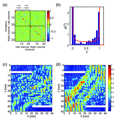
Figure 2: (a), Real part of the $\mathbf{S}$-matrix measured in the cavity [Fig. 1(a)] at $f_{0}=$0.30\text{\,}\mathrm{MHz}$$. The black lines delimit transmission and reflection matrices as depicted in Eq. (1). (b), Transmission eigenvalue histogram, $\rho\left(T\right)$, averaged over the frequency bandwidth $f=0.23-0.37$ MHz. The distribution is compared to the bimodal law $\rho_{b}\left(T\right)$ [red continuous line, Eq. (3)]. (c)-(d), Absolute values of the monochromatic wave-fields ($f_{0}=$0.30\text{\,}\mathrm{MHz}$$) associated with the two most open channels.

The $\mathbf{S}$-matrix is measured for each system with the laser-ultrasonic set-up described in Fig. 1, following the procedure explained in the Appendix A. Transmission and reflection matrices are expressed in the basis of the modes of the homogeneous plate (Gérardin et al., 2014). These eigenmodes and their eigenfrequencies have been determined theoretically using the thin elastic plate theory(Cross and Lifshitz, 2001; Santamore and Cross, 2002). They are renormalized such that each of them carries unit energy flux across the plate section(Gérardin et al., 2014). Figure 2(a) displays an example of an $\mathbf{S}$-matrix recorded at the central frequency $f_{0}=$0.30\text{\,}\mathrm{MHz}$$ for the cavity. Most of the energy emerges along the main diagonal and two sub-diagonals footnote2 of the reflection/transmission matrices. These reflection and transmission matrix elements correspond to specular reflection of each mode on the cavity boundaries and to the ballistic transmission of the incident wave-front, respectively.

We first focus on the statistics of the transmission eigenvalues $T_{l}$ computed from the measured $\mathbf{t}$-matrix (see Appendix B). Their distribution, $\rho(T)$ is estimated by averaging the corresponding histograms over the frequency bandwidth. Figure 2(b) shows the comparison between the distribution measured in the rectangular cavity and the bimodal law $\rho_{b}$ which is theoretically expected in the chaotic regimeBaranger and Mello (1994); Jalabert et al. (1994),

$$\rho_{b}\left(T\right)=\frac{1}{\pi\sqrt{T\left(1-T\right)}}$$ (3)

Even though our system is not chaotic, but exhibits regular dynamics, a good agreement is found between the measured eigenvalue distribution and the RMT predictions, confirming previous numerical studies Aigner et al. (2005). A similar bimodal distribution of transmission eigenvalues is obtained in the disordered plate, as shown in the Supplemental Material supp .

Whereas the eigenvalues $T_{l}$ of $\mathbf{tt^{{\dagger}}}$ yield the transmission coefficients of each eigenchannel, the corresponding eigenvectors provide the combination of incident modes that allow to excite this specific channel. Hence, the wave-field associated with each eigenchannel can be measured by propagating the corresponding eigenvector. To that aim, the whole system is scanned with the interferometric optical probe. A set of impulse responses is measured between the line of sources at the input and a grid of points that maps the medium. The wave function associated with a scattering state is then deduced by a coherent superposition of these responses weighted by the amplitude and phase of the eigenvector at the input (see Appendix C). Hence all the wave functions displayed in this article are only composed of experimentally measured data and do not imply any theoretical calculation or numerical simulation.

Figures 2(c) and 2(d) display the wave-field associated with the two most open eigenchannels ($T_{l}\sim 1$) of the cavity. Although such open channels allow a full transmission of the incident energy, they do not show a clear correspondence with a particular path trajectory. The same observation holds in the disordered plate supp . As a consequence, the associated scattering state undergoes multiple scattering when passing through the cavity. Figures 3(a) and 3(b) illustrate this dispersion by displaying the output temporal signal associated with the two open channels shown in Figs. 2(c) and 2(d) (see Appendix B). Both signals contain several peaks occurring at altogether three different times of flight. As we will see further, each peak is associated with a particular path trajectory and can be addressed independently by means of the Wigner-Smith time-delay matrix.

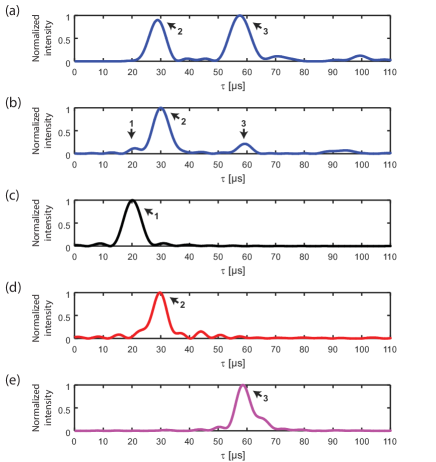
Figure 3: The time trace of a scattering or time-delay eigenstates is computed from the set of $\mathbf{t}$-matrices measured over the frequency range $f=0.23-0.37$ MHz (see Appendix B). The output intensity is displayed versus time for, (a)-(b), the two first open channels displayed in Figs. 2(c) and 2(d) and for, (c)-(e), the three time-delay eigenstates displayed in Fig. 4. For each time trace, the different echoes are labeled with a number 1, 2 or 3 that corresponds respectively, to the direct, double or quadruple scattering paths highlighted in Fig. 4.

II.2 Addressing particle-like scattering states in a cavity

The Wigner-Smith time-delay matrix $\mathbf{Q}$ is now investigated to generate coherent scattering states from the set of open channels. Since $\mathbf{Q}$ is Hermitian when derived from a unitary $\mathbf{S}$-matrix [Eq. (2)], the time-delay eigenstates $\mathbf{q}^{in}_{m}$ form an orthogonal and complete set of states, to each of which a real proper delay time $\tau_{m}$ can be assigned, such that $\mathbf{Q}\mathbf{q}^{in}_{m}=\tau_{m}\mathbf{q}^{in}_{m}$. In general, $\mathbf{q}^{in}_{m}$ is a $2N$-dimensional eigenvector which implies an injection from both the left and the right leads of the system. However, among this set of time-delay eigenstates, a subset features an incoming flux from only one lead that also exits through just one of the leads. These are exactly the desired states that belong to the subspace of open or closed channels and display trajectory-like wave function patterns.

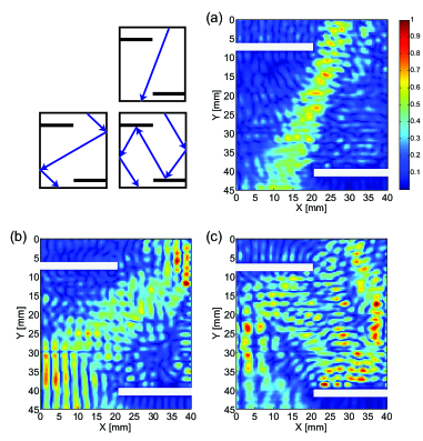
Figure 4: Absolute value of the wave-field associated with the three particle-like scattering states derived from the matrix $\mathbf{Q}$. The corresponding time delays, (a), $\tau_{m}=$20\text{\,}\mathrm{\SIUnitSymbolMicro s}$$, (b), $\tau_{m}=$30\text{\,}\mathrm{\SIUnitSymbolMicro s}$$ and, (c), $\tau_{m}=$59\text{\,}\mathrm{\SIUnitSymbolMicro s}$$, nicely match with the run-times of the corresponding classical trajectories shown in the inset (top left).

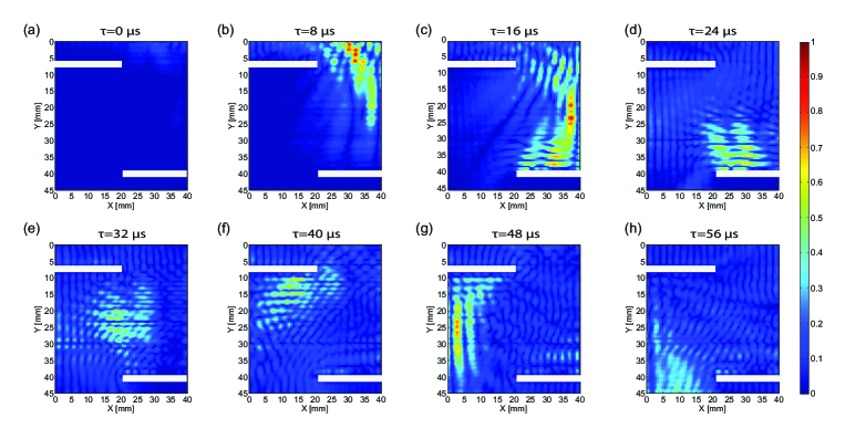
Figure 5: A spatio-temporal wave-packet is synthesized from the particle-like scattering state displayed in Fig. 4(c) over the frequency bandwidth $0.2-0.4$ MHz. The different subsets (a)-(h) display successive snapshots of its propagation across the cavity versus time.

As was shown by Rotter et al. Rotter et al. (2011), the above arguments can be translated into a straightforward operational procedure (see Appendix B), which we apply here to identify the particle-like scattering states among the time-delay eigenstates of the measured $\mathbf{Q}$-matrix. The litmus test for this procedure in the present context will be to show that the three different time traces that are identifiable in the open transmission channels [see Figs. 3(a) and 3(b)] can now be individually addressed through an associated particle-like state. The results we obtain for the cavity geometry [Fig. 1(a)] fully confirm our first successful implementation of particle-like scattering states: The propagation of the states we obtain from our procedure yields monochromatic wave states that are clearly concentrated on individual bouncing patterns [see Fig. 4]. Whereas Fig. 4(a) corresponds to the direct path between the input and output leads, Figs. 4(b) and 4(c) display a more complex trajectory with two and four reflections on the boundaries of the cavity, respectively. The associated time-delays $\tau_{m}$ do correspond to the run-times of a particle that would follow the same trajectory at the group velocity $v_{g}\sim$2.6\text{\,}\mathrm{mm}\text{\,}{\mathrm{\SIUnitSymbolMicro s}}^{-1}$$ of the flexural wave Dieulesaint and Royer (2000). Their transmission coefficients $|t_{m}|$ are equal to $0.90$, $0.95$ and $0.85$, respectively, meaning that they are almost fully transmitted through the cavity.

The time trace associated with each particle-like scattering state is computed from the frequency-dependent $\mathbf{t}$-matrix (see Appendix B). The result is displayed in Figs. 3(c), 3(d) and 3(e). Unlike the open transmission channels studied above, each particle-like state gives rise to a single pulse that arrives at the output temporally unscattered at time $\tau=\tau_{m}$. Figure 3 also shows that each temporal peak in the time trace of the open channels can be attributed to a particular path trajectory. We may thus conclude that the open channel displayed in Fig. 2(c) is mainly associated with the double and quadruple scattering paths displayed in Figs. 4(b) and 4(c). The open channel displayed in Fig. 2(d) consists of a linear combination of the paths displayed in Fig.4. This association is also confirmed by explicitly analyzing the vectorial decomposition of the particle-like state in terms of the transmission eigenchannel basis.

The frequency dependence of the particle-like scattering states is investigated in the Supplemental Material supp . They are shown to be stable over the frequency ranges $f=0.2-0.6$ MHz [Fig. 4(a)], $f=0.3-0.6$ MHz [Fig. 4(b)] and $f=0.2-0.4$ MHz [Fig. 4(c)]. The corresponding bandwidths are at least one order of magnitude larger than the frequency correlation width of the transmission matrix coefficients which is equal to 0.02 MHz supp . This proves the robustness of particle-like states over a broadband spectral range. Given this non-dispersive feature, they turn out to be perfect candidates also for the formation of minimally dispersive wave packets in the time domain. To check this conjecture, we investigate here the spatio-temporal wave functions of these states over the aforementioned bandwidths (see Appendix B). The propagation of the particle-like wave-packets through the cavity can be visualized in the three first movies of the Supplemental Material supp . Figure 5 displays successive snapshots of the wave-packet synthesized from the particle-like scattering state displayed in Fig. 4(c). Quite remarkably, the spatio-temporal focus of the incident wave-packet is maintained throughout its trajectory despite the multiple scattering events it undergoes in the cavity.

II.3 Lifting the degeneracy of particle-like scattering states

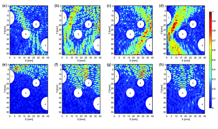
Figure 6: Absolute value of the wave-field associated with several time-delay/scattering eigenstates of the disordered system at the central frequency $f_{0}$. (a), Transmitted particle-like scattering state ($\tau_{m}=$29\text{\,}\mathrm{\SIUnitSymbolMicro s}$$, $|t_{m}|=0.84$). (b) Degenerate time-delay eigenstate mixing two particle-like trajectories ($\tau_{m}=$26\text{\,}\mathrm{\SIUnitSymbolMicro s}$$, $|t_{m}|=0.91$). (c)-(d) Unmixing of the time-delay eigenstate displayed in (b) by considering different subspaces of the $\mathbf{S}$-matrix (see Appendix D). Their transmission coefficients $|t_{m}|$ are equal to 0.94 and 0.98, respectively. (e)-(f) Closed channels deduced from the $\mathbf{S}$-matrix ($T_{l}\sim 0$) showing simultaneous reflections from the scatterers of the disordered wave guide. (g) Reflected time-delay eigenstate showing selective focusing on the scatterer n^o2 (time delay $\tau_{m}=$11\text{\,}\mathrm{\SIUnitSymbolMicro s}$$, reflection coefficient $|r_{m}|=0.94$). (h) Reflected time-delay eigenstate showing selective focusing on the scatterer n^o3 (time delay $\tau_{m}=$30\text{\,}\mathrm{\SIUnitSymbolMicro s}$$, reflection coefficient $|r_{m}|=0.88$).

In a next step, we investigate particle-like scattering states in the disordered wave guide [Fig. 1(b)]. The corresponding $\mathbf{Q}$-matrix is measured at the central frequency $f_{0}=0.3$ MHz (see Appendix A). Figures 6(a) and 6(b) display the monochromatic wave functions associated with two fully transmitted time-delay eigenstates. Whereas Fig. 6(a) displays the typical features of a particle-like scattering state that winds its way through the scatterers, the time-delay eigenstate of Fig. 6(b) is clearly associated with two scattering paths of identical length. We thus encounter here a degeneracy in the time-delay eigenvalues that needs to be lifted by an additional criterion, such as by considering well-defined subspaces of the measured $\mathbf{S}$-matrix Brandstötter (2016). In this instance, the two ray paths can be discriminated by their different angles of incidence. Correspondingly, we consider two subspaces $\mathbf{S^{\prime}}$ of the original $\mathbf{S}$-matrix by keeping either positive or negative angles of incidence from the left lead (see Appendix D). The corresponding time-delay matrices lead to two distinct particle-like scattering states displayed in Figs. 6(c) and 6(d). The two scattering paths that were previously mixed in the original time-delay eigenstate [Fig. 6(b)] are now clearly separated. The frequency stability of these states is investigated in the Supplemental Material supp . They are shown to be stable over the frequency ranges $f=0.2-0.4$ MHz [Fig. 6(c)] and $f=0.2-0.5$ MHz [Fig. 6(d)]. The corresponding particle-like wave packets are shown in the two last movies of Supplemental Material supp where the high quality of their focus in space and time is immediately apparent.

II.4 Revealing time-delay eigenstates in reflection.

Time-delay eigenstates can also result from a suitable combination of closed channels. Figures 6(e) and 6(f) display two such closed channels derived from the $\mathbf{S}$-matrix of the disordered slab. The closed channels combine multiple reflections from the holes of the scattering layer. However, the closed channel displayed in Fig. 6(e) mixes the contributions from the scatterers labeled 1 and 2. Also the closed channel displayed in Fig. 6(f) is associated with reflections from altogether three scatterers (2, 3 and 4). A simple eigenvalue decomposition of $\mathbf{rr^{{\dagger}}}$ or $\mathbf{tt^{{\dagger}}}$ does not allow a discrimination between the scatterers. On the contrary, the analysis of the $\mathbf{Q}$-matrix allows a one-to-one correspondence with each scatterer based on a time-of-flight discrimination. Figures 6(g) and 6(h) actually display the wave functions associated with two reflected time-delay eigenstates. Each of these eigenstates is associated with a reflection from a single scatterer (2 and 3, respectively). The corresponding time delays $\tau_{m}$ given in the caption of Fig. 6 are directly related to the depth $z$ of each scatterer, such that $\tau_{m}\sim 2z/v_{g}$.

III Discussion

The first point we would like to emphasize is the relevance of the time-delay matrix for selective focusing and imaging in multi-target media. The state-of-the-art approach is the DORT method (French acronym for Decomposition of the Time Reversal Operator). Initially developed for ultrasound Prada and Fink (1994); Prada et al. (1996) and more recently extended to optics Popoff et al. (2011); Badon et al. (2015), this widely used approach takes advantage of the reflection matrix $\mathbf{r}$ to focus iteratively by time reversal processing on each scatterer of a multi-target medium. Mathematically, the time-reversal invariants can be deduced from the eigenvalue decomposition of the time reversal operator $\mathbf{r}\mathbf{r^{{\dagger}}}$ or, equivalently, from the singular value decomposition of $\mathbf{r}$. On the one hand, the eigenvectors of $\mathbf{r}$ should, in principle, allow selective focusing and imaging of each scatterer. On the other hand, the associated eigenvalue directly yields the scatterer reflectivity. However, a one-to-one association between each eigenstate of $\mathbf{r}$ and each scatterer only exists under a single-scattering approximation and if the scatterers exhibit sufficiently different reflectivities. Figures 6(e) and 6(f) illustrate this limit. Because the holes display similar scattering cross-sections in the disordered slab, closed channels are associated with several scatterers at once. On the contrary, the time-delay matrix allows a discrimination between scatterers based on the time-of-flight of the reflected echoes [see Figs. 6(g) and 6(h)]. Moreover, unlike the DORT method, a time-delay analysis also allows to discriminate the single scattering paths from multiple scattering events, the latter ones corresponding to longer time-of-flights. Hence, the time-delay matrix provides an alternative and promising route for selective focusing and imaging in multi-target media.

A second relevant point to discuss is the nature of transmitted time-delay eigenstates in other complex systems. Recently, Carpenter et al. Carpenter et al. (2015) and Xiong et al. Xiong et al. (2016) investigated the group delay operator, $i/(2\pi)\mathbf{t}^{-1}\partial_{f}\mathbf{t}$, in a multi-mode optical fiber. The eigenstates of this operator are known as the principal modes in fiber optics Fan and Kahn (2005); Juarez et al. (2012). For a principal mode input, a pulse that is sufficiently narrow-band reaches the output temporally un-distorted, although it may have been strongly scattered and dispersed along the length of propagation. On the contrary, for a particle-like scattering state input, the focus of the pulse is not only retrieved at the output of the scattering medium but maintained throughout its entire propagation through the system. This crucial difference provides particle-like states with a much broader frequency stability than principal modes, which translates into the possibility to send much shorter pulses through these particle-like scattering channels. Last but not least, we also emphasize that even though particle-like states are unlikely to occur in diffusive scattering media, the time-delay eigenstates are still very relevant also in such a strongly disordered context. Consider here, e.g., that the eigenstates with the longest time delay can be of interest for energy storage, coherent absorption Chong and Stone (2011) or lasing Bachelard et al. (2012, 2014) purposes. From a more fundamental point-of-view, the trace of the $\mathbf{Q}$- matrix directly provides the density of states of the scattering medium Davy et al. (2015), a quantity that turns out to be entirely independent of the mean free path in a disordered system Pierrat et al. (2014).

Finally, we would like to stress the impact of our study on other fields of wave physics and its extension to more complex geometries. For this experimental proof-of-concept, a measurement of the wave-field inside the medium was required in order to image the wave functions and prove their particle-like feature. However, such a sophisticated protocol is not needed to physically address particle-like wave packets. A simple measurement of the scattering matrix (or a subpart of it) at neighboring frequencies Carpenter et al. (2015) yields the time-delay matrix from which particle-like state inputs can be extracted. Such a measurement can be routinely performed through 3D scattering media whether it be in optics Popoff et al. (2010); Kim et al. (2012), in the microwave regime Shi and Genack (2012); Dietz et al. (2012) or in acoustics Sprik et al. (2008); Aubry and Derode (2009). As to the generation of particle-like wave packets, multi-element technology is a powerful tool for the coherent control of acoustic waves and electromagnetic waves Mosk et al. (2012). Moreover, recent progress in optical manipulation techniques now allows for a precise spatial and temporal control of light at the input of a complex medium Mosk et al. (2012). Hence there is no obstacle for the experimental implementation of particle-like wave packets in other fields of wave physics. At last, we would like to stress the fact that in our experimental implementation we are in the limit of only a few participating modes with a wavelength that is comparable to the spatial scales of the system. In this limit the implementation of particle-like states is truly non-trivial since interference and diffraction dominates the scattering process as a whole. When transferring the concept to the optical domain one may easily reach the geometric optics limit where the wavelength is much shorter than most spatial scales of the system and particle-like states may in fact be much easier to implement in corresponding complex optical media.

IV Conclusion

In summary, we experimentally implemented particle-like scattering states in complex scattering systems. Based on an experimentally determined time-delay matrix, we have demonstrated the existence of wave packets that follow particle-like bouncing patterns in transmission through or in reflection from a complex scattering landscape. Strikingly, these wave packets have been shown to remain focused in time and space throughout their trajectory within the medium. We are convinced that the superior properties of these states in terms of frequency stability and spatial focus will make them very attractive for many applications of wave physics, ranging from focusing to imaging or communication purposes. In transmission, the efficiency of these states in terms of information transfer as well as their focused in- and output profile will be relevant. In reflection, selective focusing based on a time-of-flight discrimination will be a powerful tool to overcome aberration and multiple scattering in detection and imaging problems.

V Acknowledgments

The authors wish to thank A. Derode for fruitful discussions and advices. The authors are grateful for funding provided by LABEX WIFI (Laboratory of Excellence within the French Program Investments for the Future, ANR-10-LABX-24 and ANR-10-IDEX-0001-02 PSL*). B.G. acknowledges financial support from the French “Direction Générale de l’Armement”(DGA). P.A. and S.R. are supported by the Austrian Science Fund (FWF) through Projects NextLite F49-10 and I 1142-N27 (GePartWave).

Appendix A Experimental procedure

The first step of the experiment consists in measuring the impulse responses between two arrays of points placed on the left and right sides of the disordered slab [see Fig. 1]. These two arrays are placed 5 mm away from the disordered slab. The array pitch is $0.8$ mm (i.e $<\lambda/2$) which guarantees a satisfying spatial sampling of the wave field. Flexural waves are generated in the thermoelastic regime by a pumped diode Nd:YAG laser (THALES Diva II) providing pulses having a $20\text{\,}\mathrm{ns}$ duration and $2.5\text{\,}\mathrm{mJ}$ of energy. The out-of-plane component of the local vibration of the plate is measured with a heterodyne interferometer. This probe is sensitive to the phase shift along the path of the optical probe beam. The calibration factor for mechanical displacement normal to the surface ($100\text{\,}\mathrm{mV}\text{\,}{\mathrm{nm}}^{-1}$) was constant over the detection bandwidth ($100\text{\,}\mathrm{kHz}$ - $400\text{\,}\mathrm{kHz}$). Signals detected by the optical probe were fed into a digital sampling oscilloscope and transferred to a computer. The impulse responses between each point of the same array (left and right) form the time-dependent reflection matrices ($\mathbf{r}$ and $\mathbf{r^{\prime}}$, respectively). The set of impulse responses between the two arrays yield the time-dependent transmission matrices $\mathbf{t}$ (from left to right) and $\mathbf{t^{\prime}}$ (from right to left). From these four matrices, one can build the $\mathbf{S}$-matrix in a point-to-point basis [Eq. (1)]. A discrete Fourier transform (DFT) of $\mathbf{S}$ is then performed over a time range $\Delta t=120$ $\mu$s that excludes the echoes due to reflections on the ends of the plate and ensures that most of the energy has escaped from the sample when the measurement is stopped. The next step of the experimental procedure consists in decomposing the $\mathbf{S}$-matrices in the basis of the flexural modes of the homogeneous plate. These eigenmodes and their eigenfrequencies have been determined theoretically using the thin elastic plate theory(Cross and Lifshitz, 2001; Santamore and Cross, 2002; Gérardin et al., 2014). They are normalized such that each of them carries unit energy flux across the plate section. Theoretically, energy conservation would imply that $\mathbf{S}$ is unitary. In other words, its eigenvalues should be distributed along the unit circle in the complex plane. However, as shown in a previous work Gérardin et al. (2014), this unitarity is not retrieved experimentally because of experimental noise. A dispersion of the eigenvalues $s_{i}$ of the $\mathbf{S-}$matrix is observed around the unit circle. We compensate for this undesirable effect by considering a normalized scattering matrix with the same eigenspaces but with normalized eigenvalues Gérardin et al. (2014). The $\mathbf{Q-}$matrix is then deduced from $\mathbf{S}$ using Eq. (2). The frequency-derivative of $\mathbf{{S}}$ at $f=f_{0}$ is estimated from the centered finite difference,

$${\partial_{f}\mathbf{S}}\left(f_{0}\right)=\frac{\mathbf{S}\left(f_{0}+\delta f\right)-\mathbf{S}\left(f_{0}-\delta f\right)}{2\delta f},$$

with $\delta f=$3\text{\,}\mathrm{kHz}$$.

Appendix B Revealing transmission/time-delay eigenchannels and their temporal/spectral features

The transmission and time-delay eigenchannels are derived from the matrices $\mathbf{S}$ and $\mathbf{Q}$ measured at the central frequency $f_{0}$. The transmission matrix $\mathbf{t}(f_{0})$ (from the left to the right lead) is extracted from $\mathbf{S}(f_{0})$ [Eq. (1)]. The output and input transmission eigenvectors, $\mathbf{u}_{l}$ and $\mathbf{v}_{l}$, are derived from the singular value decomposition of $\mathbf{t}(f_{0})$:

$$\mathbf{t}(f_{0})=\sum_{l}\sqrt{T_{l}(f_{0})}\mathbf{u}_{l}(f_{0})\mathbf{v}_{l}^{{\dagger}}(f_{0})$$

with $T_{l}(f_{0})$ the intensity transmission coefficient associated with the $l^{\mbox{th}}$ scattering eigenstate at the central frequency. The frequency-dependent amplitude transmission coefficient $t_{l}\left(f\right)$ of this eigenstate can be obtained from the set of transmission matrices $\mathbf{t}\left(f\right)$ measured over the whole frequency bandwidth, such that

$$t_{l}\left(f\right)=\mathbf{u}^{{\dagger}}_{l}(f_{0})\mathbf{t}\left(f\right)\mathbf{v}_{l}(f_{0})$$

An inverse DFT of $t_{l}\left(f\right)$ finally yields the time-dependent amplitude transmission coefficient $t_{l}(\tau)$ of the $l^{\mbox{th}}$ scattering eigenstate measured at the central frequency $f_{0}$. The time traces displayed in Figs. 3(a) and 3(b) correspond to the square norm of this quantity.

The time-delay eigenchannels at the central frequency are derived from the eigenvalue decomposition of $\mathbf{Q}(f_{0})$

$$\mathbf{Q}(f_{0})=\sum_{m}{\tau_{m}}\mathbf{q}^{in}_{m}(f_{0})\left[\mathbf{q}^{in}_{m}(f_{0})\right]^{{\dagger}}$$

The time-delay eigenvector $\mathbf{q}^{in}_{m}$ is a $2N$-dimensional column vector that can be decomposed as

$$\mathbf{q}^{in}(f_{0})=\left(\begin{array}[]{c}\mathbf{q}^{in}_{m,L}(f_{0})\\ \mathbf{q}^{in}_{m,R}(f_{0})\end{array}\right)$$

where $\mathbf{q}^{in}_{m,L}(f_{0})$ and $\mathbf{q}^{in}_{m,R}(f_{0})$ contain the complex coefficients of $\mathbf{q}^{in}_{m}(f_{0})$ in the basis of the $N$ incoming modes in the left and right leads, respectively. Among the set of time-delay eigenstates, particle-like scattering states injected from the left lead should fulfill the following condition Rotter et al. (2011):

$$||\mathbf{q}_{m,L}^{in}(f_{0})||^{2}>>||\mathbf{q}_{m,R}^{in}(f_{0})||^{2}\simeq{0}.$$

A particle-like scattering state is thus associated with a $N$-dimensional input eigenvector $\mathbf{q}^{in}_{m,L}(f_{0})$. The corresponding output eigenvector $\mathbf{q}^{out}_{m,R}(f_{0})$ and transmission coefficient $t^{(q)}_{m}\left(f_{0}\right)$ can be deduced from the $\mathbf{t}$-matrix:

$$\mathbf{t}(f_{0})\mathbf{q}^{in}_{m,L}(f_{0})=t^{(q)}_{m}\left(f_{0}\right)\mathbf{q}^{out}_{m,R}(f_{0}).$$

The frequency-dependent amplitude transmission coefficient $t_{m}^{(q)}\left(f\right)$ of this time-delay eigenstate can be obtained from the set of transmission matrices $\mathbf{t}\left(f\right)$ measured over the whole frequency bandwidth, such that

$$t^{(q)}_{m}\left(f\right)=\left[\mathbf{q}^{out}_{m,L}(f_{0})\right]^{{\dagger}}\mathbf{t}\left(f\right)\mathbf{q}^{in}_{m,R}(f_{0}).$$

An inverse DFT of $t^{(q)}_{m}\left(f\right)$ finally yields the time-dependent amplitude transmission coefficient $t^{(q)}_{m}(\tau)$ of the $m^{\mbox{th}}$ time-delay eigenstate measured at the central frequency $f_{0}$. The time traces displayed in Figs. 3(c), 3(d) and 3(e) correspond to the square norm of this quantity.

Appendix C Imaging spatio-temporal wave functions of transmission/reflection and time-delay eigenchannels

Impulse responses are measured between the line of sources (denoted by the index $i$) and a grid of points (denoted by the index $j$) that maps the medium, following the same procedure as the one described above. The grid pitch is 1.3 mm. This set of impulse responses forms a transmission matrix $\mathbf{k}(\tau)=[k_{ji}(\tau)]$. A discrete Fourier transform (DFT) of $\mathbf{k}(\tau)$ yields a set of frequency-dependent transmission matrices $\mathbf{k}(f)$. The lines of $\mathbf{k}(f)$ are then decomposed in the basis of the plate modes. The monochromatic wave-field $\mathbf{\Psi}(f)=[\psi_{j}(f)]$ associated with a transmission/reflection or time-delay eigenchannel is provided by the product between the matrix $\mathbf{k}(f)$ and the corresponding eigenvector ($\mathbf{v}_{l}(f_{0})$ or $\mathbf{q}^{in}_{m,L}(f_{0})$, respectively). The time-dependent wave-field $\mathbf{\Psi}(\tau)=[\psi_{j}(\tau)]$ is deduced by an inverse DFT over a frequency bandwidth of our choice. Note that a Hann window function is priorly applied to $\mathbf{k}(f)$ to limit side lobes in the time-domain.

Appendix D Unmixing degenerated time-delay eigenstates.

Depending on the geometry of the scattering medium, the different scattering paths involved in a degenerated time-delay eigenstate can be discriminated either in the real space or in the spatial frequency domain Brandstötter (2016). Here, the time-delay eigenstate displayed in Fig. 6(b) shows two scattering paths with opposite angles of incidence. Hence, they can be discriminated by analyzing each block of the $\mathbf{S}$-matrix in the spatial frequency domain. The left lead of each block is decomposed over the positive or negative angles of incidence. This sub-space of the $\mathbf{S}$-matrix, refered to as $\mathbf{S^{\prime}}$, is then used to compute a reduced time-delay matrix $\mathbf{Q^{\prime}}$ Brandstötter (2016) such that

$$\mathbf{Q^{\prime}}=-\frac{i}{2\pi}\mathbf{S^{\prime}}^{-1}\partial_{f}\mathbf{S^{\prime}}.$$

Note that the transpose conjugate operation of Eq. (2) is here replaced by an inversion of $\mathbf{S^{\prime}}$ because of its non-unitarity Brandstötter (2016). Depending on the sign of the angle of incidence chosen for the left lead, the reduced matrix $\mathbf{Q^{\prime}}$ provides the time-delay eigenstates displayed in Figs. 6(c) and 6(d).

Supplemental Material

This document provides further information on the scattering matrix measured in the disordered wave guide and the stability of particle-like states in the frequency domain. The captions of the Supplementary Movies are also listed at the end of the document.

Appendix A Scattering matrix analysis in the disordered waveguide

Figure S1(a) displays an example of $\mathbf{S-}$matrix recorded in the disordered wave guide depicted in Fig. 1(a) of the accompanying paper. Despite a moderate level of disorder, the $\mathbf{S}-$matrix exhibits an overall random appearance. Nevertheless, a residual ballistic wave-front slightly emerges along the diagonal of the transmission matrices.

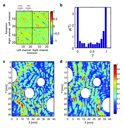
Figure S1: (a), Amplitude of the $\mathbf{S-}$matrix measured in the scattering slab at $f_{0}=$0.30\text{\,}\mathrm{MHz}$$. The black lines delimit transmission and reflection matrices. (b), Transmission eigenvalue histograms, $\rho\left(T\right)$, averaged over the frequency bandwidth. (c)-(d), Absolute value of the monochromatic wave-fields associated with two open channels at the central frequency.

The statistics of the transmission eigenvalues $T_{l}$ computed from the $\mathbf{t-}$matrix is now investigated. As for the regular cavity, their distribution $\rho\left(T\right)$ is estimated by averaging their histograms over the frequency bandwidth. Fig. S1(b) displays the estimator of this distribution. Most of the transmission coefficients are found to be either close to zero or one, accounting respectively for closed and open channels. Figures S1(c) and S1(d) display the wave-fields associated with two open channels at the central frequency (see Methods). As in the cavity, the open channels combine multiple path trajectories. As a consequence, they undergo a strong spatial and temporal dispersion while propagating through the scattering slab. As shown in Fig.6 of the accompanying paper, the study of the time-delay matrix allows to lift this degeneracy.

Appendix B Stability of the particle-like states in the frequency domain

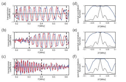
Figure S2: (a)-(b)-(c), Frequency dependence of the transmission coefficients $t^{(q)}_{m}(f)$ for the three cavity particle-like states displayed in Fig. 4(a)-(b)-(c), respectively (blue line: real part, red line: imaginary part). The black vertical dashed lines delimit the bandwidth of each state. (d)-(e)-(f), Spectral correlation function $|C_{m}(\delta f)|$ (blue line) of the transmission coefficient $t^{(q)}_{m}(f)$ displayed in (a)-(b)-(c), respectively. $C_{m}(\delta f)$ is computed by considering the central frequency $f_{0}$ of each state. Each curve is compared with the spectral correlation function $C(\delta f)$ of the transmission matrix elements (black dashed line).

Figures S2(a) and S2(c) display the frequency dependence of the transmission coefficients $t^{(q)}_{m}(f)$ for the three cavity particle-like states displayed in Fig. 4. The frequency evolution of $t^{(q)}_{m}(f)$ allows to delimit the frequency range over which each particle-like state remains stable: $f=0.2-0.6$ MHz [Fig. S2(a)], $f=0.3-0.6$ MHz [Fig. S2(b)] and $f=0.2-0.4$ MHz [Fig. S2(c)]. To be more quantitative, we have estimated the spectral correlation function of each state,

$$C_{m}(\delta f)=t^{(q)}_{m}(f_{0})t^{(q)*}_{m}(f_{0}+\delta f),$$

with $f_{0}$ the associated central frequency. The result is displayed in Figs. S2(d), S2(e) and S2(f), and compared to the mean spectral correlation function,

$$C(\delta f)=\left\langle t_{ij}(f)t^{*}_{ij}(f+\delta f)\right\rangle,$$

of the measured transmission matrix coefficients $t_{ij}(f)$. The symbol $\langle.\rangle$ here denotes an average over the frequency bandwidth. The FWHM of $C_{m}(\delta f)$ yields the spectral correlation width $\delta f_{m}$ of each state displayed in Fig. 4. We find $\delta f_{m}=$ 0.16 MHz [Fig. S2(d)], 0.17 MHz [Fig. S2(e)] and 0.12 MHz [Fig. S2(f)]. These values should be compared to the frequency correlation width $\delta f_{c}=0.02$ MHz of the transmission matrix coefficients. We see that the spectral correlation width $\delta f_{m}$ of particle-like states is 8, 8.5 and 6 times larger than $\delta f_{c}$. This illustrates the stability of the cavity particle-like states in the frequency domain and accounts for the spatio-temporal focusing of particle-like wave packets in the time domain (see Supplementary Movies 1, 2 and 3).

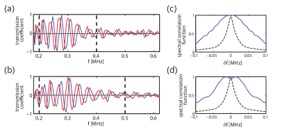
Figure S3: (a)-(b), Frequency dependence of the transmission coefficients $t^{q}_{m}(f)$ for the two particle-like states in the disordered wave guide, displayed in Figs. 6(c) and 6(d), respectively (blue line: real part, red line: imaginary part). The black vertical dashed lines delimit the bandwidth of each state. (c)-(d), Spectral correlation function, $|C_{m}(\delta_{f})|$, for the transmission coefficient $t^{q}_{m}(f)$ displayed in (a)-(b), respectively. $C_{m}(\delta f)$ is computed by considering the central frequency $f_{0}$ of each state. Each curve is compared with the spectral correlation function $|C(\delta f)|$ of the transmission matrix elements (black dashed line).

The same analysis can be performed for the disordered wave guide. As an example, we investigate the frequency stability of the particle-like states displayed in Figs.6(c) and 6(d). Figures S3(a) and S3(b) display the frequency dependence of the corresponding transmission coefficients $t^{(q)}_{m}(f)$. Each state remains stable over a frequency range $f=0.2-0.4$ MHz [Fig.S3(a)] and $f=0.2-0.5$ MHz [Fig.S3(b)]. The corresponding spectral correlation functions $C_{m}(\delta f)$ are displayed in Figs.S3(c) and S3(d). We measure a frequency correlation width $\delta f_{m}$ of 0.13 and 0.12 MHz. Contrastingly, the transmission matrix elements exhibit a frequency correlation width $\delta f_{c}=0.025$ MHz. $\delta f_{m}$ is thus 5 times higher than $\delta f_{c}$. This demonstrates the frequency stability of these two particle-like states and accounts for the spatio-temporal focusing of the corresponding particle-like wave packets in the time domain (see Supplementary Movies 4 and 5).

Appendix C Captions of the Supplementary Movies

Movie 1: Particle-like wave-packet in the cavity synthesized from the scattering state displayed in Fig. 4(a) over the frequency range $f=0.2-0.6$ MHz.

Movie 2: Particle-like wave-packet in the cavity synthesized from the scattering state displayed in Fig. 4(b) over the frequency range $f=0.3-0.6$ MHz.

Movie 3: Particle-like wave-packet in the cavity synthesized from the scattering state displayed in Fig. 4(c) over the frequency range $f=0.2-0.4$ MHz.

Movie 4: Particle-like wave-packet in the disordered wave guide synthesized from the scattering state displayed in Fig. 6(c) over the frequency range $f=0.2-0.4$ MHz.

Movie 5: Particle-like wave-packet in the disordered wave guide synthesized from the scattering state displayed in Fig. 6(d) over the frequency range $f=0.2-0.5$ MHz.

References

- Derode et al. (1995) A. Derode, P. Roux, and M. Fink, “Robust acoustic time reversal with high-order multiple scattering,” Phys. Rev. Lett. 75, 4206–4209 (1995).
- Tanter et al. (2000) M. Tanter, J.-L. Thomas, and M. Fink, “Time reversal and the inverse filter,” J. Acoust. Soc. Am. 108, 223–234 (2000).
- Lerosey et al. (2004) G. Lerosey, J. de Rosny, A. Tourin, A. Derode, G. Montaldo, and M. Fink, “Time reversal of electromagnetic waves,” Phys.Rev. Lett. 92, 193904 (2004).
- Lerosey et al. (2007) G. Lerosey, J. de Rosny, A. Tourin, and M. Fink, “Focusing beyond the diffraction limit with far-field time reversal,” Science 315, 1120–1122 (2007).
- Vellekoop and Mosk (2007) I. M. Vellekoop and A. P. Mosk, “Focusing coherent light through opaque strongly scattering media,” Opt. Lett. 32, 2309–2311 (2007).
- Popoff et al. (2010) S. M. Popoff, G. Lerosey, R. Carminati, M. Fink, A. C. Boccara, and S. Gigan, “Measuring the Transmission Matrix in Optics: An Approach to the Study and Control of Light Propagation in Disordered Media,” Phys. Rev. Lett. 104, 100601 (2010).
- Aulbach et al. (2011) J. Aulbach, B. Gjonaj, P. M. Johnson, A. P. Mosk, and A. Lagendijk, “Control of light transmission through opaque scattering media in space and time,” Phys. Rev. Lett. 106, 103901 (2011).
- McCabe et al. (2011) D. J. McCabe, A. Tajalli, D. R. Austin, P. Bondareff, I. A. Walmsley, S. Gigan, and B. Chatel, “Spatio-temporal focussing of an ultrafast pulse through a multiply scattering medium,” Nature Commun. 2, 447 (2011).
- Katz et al. (2011) O. Katz, E. Small, Y. Bromberg, and Y. Silberberg, “Focusing and compression of ultrashort pulses through scattering media,” Nature Photon. 5, 371–377 (2011).
- Vellekoop and Mosk (2008) I. M. Vellekoop and A. P. Mosk, “Universal optimal transmission of light through disordered materials,” Phys. Rev. Lett. 101, 120601 (2008).
- Pendry (2008) J. B. Pendry, “Light finds a way through the maze,” Physics 1, 20 (2008).
- Kim et al. (2012) M. Kim, Y. Choi, C. Yoon, W. Choi, J. Kim, Q-H. Park, and W. Choi, “Maximal energy transport through disordered media with the implementation of transmission eigenchannels,” Nature Photon. 6, 583–587 (2012).
- Shi and Genack (2012) Z. Shi and A. Genack, “Transmission eigenvalues and the bare conductance in the crossover to anderson localization,” Phys. Rev. Lett. 108, 043901 (2012).
- Choi et al. (2011) W. Choi, A. P. Mosk, Q.-H. Park, and W. Choi, “Transmission eigenchannels in a disordered medium,” Phys. Rev. B 83, 134207 (2011).
- Gérardin et al. (2014) B. Gérardin, J. Laurent, A. Derode, C. Prada, and A. Aubry, “Full transmission and reflection of waves propagating through a maze of disorder,” Phys. Rev. Lett. 113, 173901 (2014).
- Hsu et al. (2015) C. W. Hsu, A. Goestschy, Y. Bromberg, A. D. Stone, and H. Cao, “Broadband coherent enhancement of transmission and absorption in disordered media,” Phys. Rev. Lett. 115, 223901 (2015).
- Rotter et al. (2011) S. Rotter, P. Ambichl, and F. Libisch, “Generating particlelike scattering states in wave transport,” Phys. Rev. Lett. 106, 120602 (2011).
- Aubry et al. (2008) J.-F. Aubry, M. Pernot, F. Marquet, M. Tanter, and M. Fink, “Transcostal high-intensity-focused ultrasound: ex vivo adaptive focusing feasibility study,” Phys. Med. Biol. 53, 2937–2951 (2008).
- Cochard et al. (2009) E. Cochard, C. Prada, J.-F. Aubry, and M. Fink, “Ultrasonic focusing through the ribs using the dort method,” Med. Phys. 36, 3495–3503 (2009).
- Edelmann et al. (2002) G. F. Edelmann, T. Akal, W. S. Hodgkiss, S. Kim, W. A. Kuperman, and H. C. Song, “An initial demonstration of underwater acoustic communication using time reversal,” IEEE J. Ocean. Eng. 27, 602–609 (2002).
- Prada et al. (2007) C. Prada, J. de Rosny, D. Clorennec, J.-G. Minonzio, A. Aubry, M. Fink, L. Berniere, P. Billand, S. Hibral, and T. Folegot, “Experimental detection and focusing in shallow water by decomposition of the time reversal operator,” J. Acoust. Soc. Am. 122, 761–768 (2007).
- Cizmar and Dholakia (2012) T. Cizmar and K. Dholakia, “Exploiting multimode waveguides for pure fibre-based imaging,” Nature Comm. 3, 1027 (2012).
- Papadopoulos et al. (2012) I. N. Papadopoulos, S. Farahi, C. Moser, and D. Psaltis, “Focusing and scanning light through a multimode optical fiber using digital phase conjugation,” Opt. Exp. 20, 10583–10590 (2012).
- Plöschner et al. (2015) M. Plöschner, T. Tyc, and T. Cizmàr, “Seeing through chaos in multimode fibres,” Nature Photon. 9, 529–535 (2015).
- Fan and Kahn (2005) S. Fan and J. M. Kahn, “Principal modes in multimode waveguides,” Opt. Lett. 30, 135–137 (2005).
- Juarez et al. (2012) A. A. Juarez, C. A. Bunge, S. Warm, and K. Petermann, “Perspectives of principal mode transmission in mode-division-multiplex operation,” Opt. Exp. 20, 13810–13823 (2012).
- Carpenter et al. (2015) J. Carpenter, B. J. Eggleton, and J. Schröder, “Observation of eisenbud–wigner–smith states as principal modes in multimode fibre,” Nature Photon. 9, 751–757 (2015).
- Xiong et al. (2016) W. Xiong, P. Ambichl, Y. Bromberg, S. Rotter, and H. Cao, “Spatio-temporal control of light transmission through a multimode fiber with strong mode coupling,” arXiv:1601.04646 (2016) [Phys. Rev. Lett., in press].
- Carpenter and Wilkinson (2012) B. C. Carpenter, J. Thomsen and T. D. Wilkinson, “Degenerate mode-group division multiplexing,” J. Lightw. Technol. 30, 3946–3952 (2012).
- Salz (1985) J. Salz, “Digital transmission over cross-coupled linear channels,” At&T Technical Journal 64, 1147–1159 (1985).
- Raleigh and Cioffi (1998) G. G. Raleigh and J. M. Cioffi, “Spatio-temporal coding for wireless communication,” Communications, IEEE Transactions on 46, 357–366 (1998).
- Tulino and Verdù (2004) A. Tulino and S. Verdù, “Random matrix theory and wireless communications,” Fundations and Trends in Communications and Information Theory 1, 1–182 (2004).
- Sprik et al. (2008) R. Sprik, A. Tourin, J. de Rosny, and M. Fink, “Eigenvalue distributions of correlated multichannel transfer matrices in strongly scattering systems,” Phys. Rev. B 78, 012202 (2008).
- Aubry and Derode (2009) A. Aubry and A. Derode, “Random Matrix Theory Applied to Acoustic Backscattering and Imaging In Complex Media,” Phys. Rev. Lett. 102, 084301 (2009).
- Dietz et al. (2012) O. Dietz, H.-J. Stöckmann, U. Kuhl, F. M. Izrailev, N. M. Makarov, J. Doppler, F. Libisch, and S. Rotter, “Surface scattering and band gaps in rough waveguides and nanowires,” Phys. Rev. B 86, 201106 (2012).
- Beenakker (1997) C. W. J. Beenakker, “Random-matrix theory of quantum transport,” Rev. Mod. Phys. 69, 731–808 (1997).
- (37) The symbol here stands for transpose conjugate.
- Dorokhov (1984) O. N. Dorokhov, “On the coexistence of localized and extended electronic states in the metallic phase,” Sol. St. Comm. 51, 381–384 (1984).
- Imry (1986) Y. Imry, “Active transmission channels and universal conductance fluctuations,” Europhys. Lett. 1, 249–256 (1986).
- Baranger and Mello (1994) H. U. Baranger and P. A. Mello, “Mesoscopic transport through chaotic cavities: A random s-matrix theory approach,” Phys. Rev. Lett. 73, 142–145 (1994).
- Jalabert et al. (1994) R. A. Jalabert, J.-L. Pichard, and C. W. J. Beenakker, “Universal quantum signatures of chaos in ballistic transport,” Europhys. Lett. 27, 255–260 (1994).
- Wigner (1955) E. P. Wigner, “Lower limit for the energy derivative of the scattering phase shift,” Phys. Rev. 98, 145–147 (1955).
- Smith (1960) F. T. Smith, “Lifetime matrix in collision theory,” Phys. Rev. 118, 349–356 (1960).
- Prada and Fink (1994) C. Prada and M. Fink, “Eigenmodes of the time reversal operator: A solution to selective focusing in multiple-target media,” Wave Motion 20, 151–163 (1994).
- Prada et al. (1996) C. Prada, S. Manneville, D. Spoliansky, and M. Fink, “Decomposition of the time reversal operator: Detection and selective focusing on two scatterers,” J. Acoust. Soc. Am. 99, 2067–2076 (1996).
- Popoff et al. (2011) S. M. Popoff, A. Aubry, G. Lerosey, M. Fink, A. C. Boccara, and S. Gigan, “Exploiting the time-reversal operator for adaptive optics, selective focusing, and scattering pattern analysis,” Phys. Rev. Lett. 107, 263901 (2011).
- Badon et al. (2015) A. Badon, D. Li, G. Lerosey, A. C. Boccara, M. Fink, and A. Aubry, “Smart optical coherence tomography for ultra-deep imaging through highly scattering media,” arXiv:1510.08613 (2015).
- Cross and Lifshitz (2001) M. C. Cross and R. Lifshitz, “Elastic wave transmission at an abrupt junction in a thin plate with application to heat transport and vibrations in mesoscopic systems,” Phys. Rev. B 64, 085324 (2001).
- Santamore and Cross (2002) D. H. Santamore and M. C. Cross, “Surface scattering analysis of phonon transport in the quantum limit using an elastic model,” Phys. Rev. B 66, 144302 (2002).
- (50) The more energetic sub-diagonals of the transmission/reflection matrices account for the conversion between even and odd modes of similar momentum.
- Aigner et al. (2005) F. Aigner, S. Rotter, and J. Burgdörfer, “Shot noise in the chaotic-to-regular crossover regime,” Phys. Rev. Lett. 94, 216801 (2005).
- (52) See Supplemental Material which includes the scattering matrix analysis of the disordered waveguide, the frequency study of particlelike scattering states and five movies showing particle-like wave packets propagating through the cavity and the disordered waveguide.
- Dieulesaint and Royer (2000) E. Dieulesaint and D. Royer, Elastic waves in solids I (Springer-Verlag, Berlin, 2000).
- Brandstötter (2016) Andre Brandstötter, Master’s thesis, Institute for Theoretical Physics - Vienna University of Technology (2016).
- Chong and Stone (2011) Y. D. Chong and A. D. Stone, “Hidden black: Coherent enhancement of absorption in strongly scattering media,” Phys. Rev. Lett. 107, 163901 (2011).
- Bachelard et al. (2012) N. Bachelard, J. Andreasen, S. Gigan, and P. Sebbah, “Taming random lasers through active spatial control of the pump,” Phys. Rev. Lett. 109, 033903 (2012).
- Bachelard et al. (2014) N. Bachelard, S. Gigan, X. Noblin, and P. Sebbah, “Adaptive pumping for spectral control of random lasers,” Nature Phys. 10, 426–431 (2014).
- Davy et al. (2015) M. Davy, Z. Shi, J. Wang, X. Cheng, and A. Z. Genack, “Transmission eigenchannels and the densities of states of random media,” Phys. Rev. Lett. 114, 033901 (2015).
- Pierrat et al. (2014) R. Pierrat, P. Ambichl, S. Gigan, A. Haber, R. Carminati, and S. Rotter, “Invariance property of wave scattering through disordered media,” Proc. Nat. Acad. Sci. U.S.A. 111, 17765–17770 (2014).
- Mosk et al. (2012) A. P. Mosk, A. Lagendijk, G. Lerosey, and M. Fink, “Controlling waves in space and time for imaging and focusing in complex media,” Nature Photon. 6, 283–292 (2012).