A fast platform for simulating flexible fiber suspensions
applied to cell mechanics

Abstract

We present a novel platform for the large-scale simulation of fibrous structures immersed in a Stokesian fluid and evolving under confinement or in free-space. One of the main motivations for this work is to study the dynamics of fiber assemblies within biological cells. For this, we also incorporate the key biophysical elements that determine the dynamics of these assemblies, which include the polymerization and depolymerization kinetics of fibers, their interactions with molecular motors and other objects, their flexibility, and hydrodynamic coupling.

This work, to our knowledge, is the first technique to include many-body hydrodynamic interactions (HIs), and the resulting fluid flows, in cellular fiber assemblies. We use the non-local slender body theory to compute the fluid-structure interactions of the fibers and a second-kind boundary integral formulation for other rigid bodies and the confining boundary. A kernel-independent implementation of the fast multiple method is utilized for efficient evaluation of HIs. The deformation of the fibers is described by the nonlinear Euler–Bernoulli beam theory and their polymerization is modeled by the reparametrization of the dynamic equations in the appropriate non-Lagrangian frame. We use a pseudo-spectral representation of fiber positions and implicit HIs in the time-stepping to resolve large fiber deformations, and to allow time-steps not constrained by temporal stiffness or fiber-fiber interactions. The entire computational scheme is parallelized, which enables simulating assemblies of thousands of fibers. We use our method to investigate two important questions in the mechanics of cell division: (i) the effect of confinement on the hydrodynamic mobility of microtubule asters; and (ii) the dynamics of the positioning of mitotic spindle in complex cell geometries. Finally to demonstrate the general applicability of the method, we simulate the sedimentation of a cloud of fibers.

1 Introduction

Semi-flexible biopolymers constitute a principal mechanical component of intracellular structures [6, 65, 5]. Together with molecular motors, fiber networks, consisting of such polymers, form the cytoskeleton that is the cell’s mechanical machinery for executing several key tasks including cell motility, material transport, and cell division [40]. From these semi-flexible filaments (microtubules, actin filaments and intermediate filaments) and a variety of molecular motors the cytoskeleton is able to reorganize to supramolecular architectures that are distinctly designed to perform a particular task [25, 40].

Due to their central role in intracellular structures the rheology and collective dynamics of semi-flexible fiber suspensions and networks has attracted increasing interest in engineering and biology [6].

The basic physical difference between semi-flexible fibers and their better-understood counterpart, polymer chains, is the significantly larger bending rigidity of fibers that then yields larger end-to-end distances. This results in many interesting differences between the rheology of semi-flexible polymers and that of the two extreme limits of flexibility, polymer melts and rigid fiber suspensions. For example, the stiffness of semi-flexible networks can increase or decrease under compression and their suspensions show negative normal stress differences [65, 6, 9].

With advancements in microscopy and data acquisition at small time- and length-scales, we now know a great deal about the interactions of the individual microscopic filaments and their associated motor proteins. On the other hand, we know very little about how they interact collectively and how these interactions determine the ensemble behavior of cellular matter and structures.

Microrheological measurements provide a strong basis for understanding the mechanical behavior of cytoskeletal structures and matter [106, 65, 94], but do not directly inform us of the relationship between microscopic interactions and macroscopic behaviors. Moreover, living systems typically operate far from equilibrium—due to internally generated forces being much larger than thermal forces—and constitutive relationship is required to extract rheological behavior based on, for example, the trajectories of probe particles. Finding microscopic constitutive relations is difficult even for the simplest of out-of-equilibrium complex fluids, a hard-sphere colloidal suspension, due to the complex and nonlinear relations between rheological properties and microstructural dynamics [70].

Dynamic simulation is a powerful tool to gain insight into the underlying physical principles that govern the formation and reorganization of cytoskeletal structures and ultimately obtain relevant constitutive relationships. With the continuous advancements in in vitro reconstitution of cellular matter, comparing the experiments with in silico reconstitution (i.e., detailed, large-scale, dynamic simulation of cellular structures) is within reach [5]. To this end, this paper presents a computational platform for dynamic simulation of semi-flexible fiber suspensions in Stokes flow. Our method explicitly accounts for fiber flexibility, their polymerization and depolymerization kinetics, their interactions with molecular motors, and hydrodynamic interactions (HIs). From a physical point of view, what distinguishes our method is the inclusion of HIs, which has been almost entirely ignored in the previous theoretical and numerical studies of cellular structures [6].

We consider suspensions of hydrodynamically interacting rigid bodies and flexible fibers immersed in a Stokesian fluid, either under confinement or in free-space. Our approach is based upon boundary integral formulations of solutions to the Stokes equations. The flows associated with the motion of rigid bodies and confining surfaces are represented through a well-conditioned second-kind boundary integral formulation [75]. The fluid flows associated with the dynamics of fibers are accounted for using non-local slender body theory [50, 44, 31, 102].

Related work

Modeling approaches to suspensions and networks of fibers can be roughly categorized into volume- and particle-based methods. In volume-based methods, the Stokes (or Navier–Stokes) equation is solved by discretizing the entire computational domain. Within this class, immersed boundary methods have been applied to study the dynamics of single [91, 54] or several [109] flexible fibers. The fibers are typically represented by a discrete set of points (forming a one-dimensional curve [91, 109], or a three-dimensional cylinder [54]) whose interactions capture stretching stiffness and internal elastic stresses.

These points on the fibers are Lagrangian and so are moved with the background fluid flow. The consequent stretching or bending of the discretized fiber creates elastic forces represented at the Lagrangian points. These forces are distributed to the background grid, which then provides forcing terms solving anew the Stokes or Navier–Stokes equations for the updated background flow. This cycle is then repeated. A similar update strategy has been adopted using the Lattice Boltzmann method [104] to study the rheology of flexible fiber suspensions. Typically, to properly account for fluid-structure interactions in volume-based methods, the size of the volume grid is taken to be several times smaller than the smallest dimension of the immersed bodies. As a result, these methods become computationally expensive for simulating slender bodies such as fibers and disks. Moreover, these methods typically use explicit time-stepping to evolve fiber shapes and elastic forces that substantially limits the region of time-step stability [55] due to temporal stiffness.

Versions of particle-based methods include bead-spring models, regularized Stokes, variations of dissipative particle dynamics [18, 33], and slender-body theory (which we use in this work). In bead-spring models, the fiber is represented as a chain of rigid spheres [112, 113, 26] or ellipsoids [85] linked by inextensible connectors with finite bending rigidity [43] or by springs with given tensile and bending stiffnesses [85, 68]. The system is evolved by imposing the balance between hydrodynamic and elastic forces and torques on all beads. Some implementations of this method include long-range hydrodynamics as well as short-range lubrication interactions [112, 113, 43], while others only include local drag on the beads [85]. The advantage of these techniques is their relatively simple implementation. Due to the discreteness of the fiber in this construction, the polymerization of fibers is captured by adding and removing beads and springs discretely in time [68].

Alternatively, the Regularized Stokes Method (RSM) [16, 14] has been used to model the dynamics of elastic fibers in Stokes flow [24, 95, 73]. The RSM represents the fluid velocity as the superposition of smoothed fundamental solutions to the Stokes equation, with spread $\delta$, distributed on immersed surfaces [14]. To be convergent, this method needs area elements to be scaled proportionally to $\delta^{2}$ [14]. Smith [95] removed this constraint by formulating the integrals in the context of a boundary element method. Flores et al. [24] used this framework to study the role of hydrodynamic interactions on the dynamics of flagella. Olson et al. [73] combined the elastic rod model developed by [54] with the RSM to study the dynamics of rods with intrinsic curvature and twist. In the context of fibers, the RSM is similar to slender body theory but to achieve the same order of accuracy in velocity as in slender body theory, the regularization factor $\delta$ needs to be in the order of the aspect ratio of the fibers. This becomes computationally demanding for slender objects.

In Boundary Integral (BI) methods, the Stokes equation is recast in the form of integrals of distributions of point forces, torques, and stresses on the boundaries of the fluid domain. As a result, the computational domain is reduced to the two-dimensions of the immersed surfaces. In Slender Body Theory (SBT), the slenderness of the fiber is used to asymptotically reduce the BI formulation to one-dimensional integrals along the fibers’ centerlines. This results in non-local slender body theory (NLSBT) [50, 44, 31, 102], which is asymptotically accurate to $\mathcal{O}\left(\epsilon^{2}\log\epsilon\right)$, where $\epsilon\ll 1$ is the aspect ratio of the fiber. Shelley and Ueda [97] designed numerical methods for simulating closed flexible fibers based on NLSBT which [102] extended substantially to fibers with free ends and devised algorithms to make the problem tractable and numerically stable.

Contributions

We extend [102] to enable simulation of $\mathcal{O}(1000)$ actively driven semi-flexible filaments. To achieve this, we introduce several enhancements:

• Spectral spatial discretization: A Chebyshev basis is used for the representation of fiber position enabling us to compute high-order derivatives with uniform accuracy along the fiber.

• Fiber (de)polymerization: In biological settings the polymerization/depolymerization of biopolymers is a crucial part of their dynamics. Here we account for this dynamics by reparametrization of the dynamic equations into a non-Lagrangian frame. We found this formulation to be considerably more stable (at least in our setting) compared to introducing segments at discrete moments in time, as done in [68].

• Removing numerical stiffness: In the [102] framework, to remove temporal stiffness, the bending forces were treated implicitly, while the tension equation—which imposed inextensibility of the fibers—was treated explicitly. We found that this formulation imposes severe limitations on the time-step magnitude for large numbers of fibers. In our method, both bending and tensile forces are treated implicitly. As a result, the time-step in our scheme shows no dependency on the number of points per fiber and is only weakly dependent on the number of fibers.

• Computational cost of $\mathcal{O}(N)$ and full parallelization: Due to implicit treatment of the HIs and use of a BI method, at each time-step a dense system of equations must be solved. We solve this system using GMRES with a Jacobi or block Jacobi preconditioner. A kernel independent fast multipole method (FMM) [110, 57] is utilized for fast computation of nonlocal hydrodynamic interactions, and fast matrix-vector products. The combination of GMRES, efficient preconditioning, and FMM results in $\mathcal{O}(N)$ computational cost per time-step, where $N$ is the number of unknowns, approximately proportional to the number of fibers. Due to implicit treatment of bending and tensile forces as well as the HIs, the stable time-step is three orders of magnitude larger than the stable time-step for the explicit method. The entire computational scheme, including the FMM routine, the matrix-vector operations in GMRES, are parallelized and scalable to many computational cores.

To test our scheme and to demonstrate the variety of problems that can be studied within this framework, we considered three representative problems. We first investigate the mobility and viscoelastic behavior of a spherical particle surrounded by a fibrous shell and compare our results with analytical results obtained by using the porous medium Brinkman model for the shell [8, 64]. Through this example we clearly demonstrate that HIs play a critical role in setting the dynamics of fibrous networks.

As an application of the current framework to cellular mechanics, we study the effect of cell geometry on the positioning of the pronuclear complex (PNC) in the prophase stage of cell division in C. elegans [15]. For this purpose, we consider three cell geometries and two different proposed force transduction mechanisms for moving the PNC. We demonstrate that changing the geometry of the cell and the forcing mechanism both result in substantial changes in the PNC positioning dynamics.

To demonstrate the utility of our method beyond biological settings, we then look at the sedimentation of a cloud of flexible fibers, a classical suspension mechanics problem. We find that the many-body hydrodynamic interactions rearrange the fibers, resulting in evolution of the cloud into a torus-like structure.

Our simulation results in all three problems are consistent with available theoretical predictions and previous experimental and simulation results. More importantly, our study of each problem revealed several other interesting directions of research which can be pursued within our framework.

2 Formulation

Consider a suspension of $N_{F}$ elastic fibers and $N_{P}$ rigid particles immersed in a Newtonian fluid which is either confined by an outer boundary $\Gamma_{0}$ or which fills free space. The effect of thermal fluctuations on the fibers and other immersed bodies are neglected throughout this work. In the context of intracellular assemblies, the confining boundary represents a cell wall, and the Newtonian fluid filling the cell is the cytoplasm that envelopes the assembly of the microscopic filaments, nuclear complexes, and other organelles. A schematic is shown in Fig. 1.

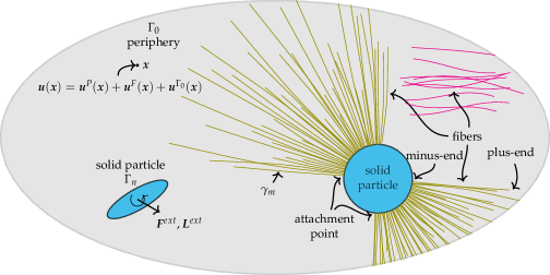
Figure 1: Schematic. The gray-shaded region denotes the fluid domain $\Omega$. The outer boundary is denoted by $\Gamma_{0}$. There are rigid particles and flexible fibers suspended within the domain. The fibers and particles interact hydrodynamically with each other. Fibers may be attached to particles by different means that are specified through the boundary conditions on their ends (e.g. hinged or clamped). When attached, fibers exert force $\bm{F}^{ext}$ and torque $\bm{L}^{ext}$ upon rigid particles. Fibers can also move freely or sediment within the fluid domain. The velocity at a point $\bm{x}\in\Omega$ results from the motion of particles $\bm{u}^{P}$, fibers $\bm{u}^{F}$, and the backflow due to the confinement $\bm{u}^{\Gamma_{0}}$.

The ratio of inertial to viscous forces is the Reynolds number, $Re=\rho Lu/\mu$, where $\rho$ and $\mu$ are the cytoplasmic density and viscosity, respectively, $L$ is the characteristic length of the cell, and $u$ is an average velocity magnitude. For cellular flows, due to the high viscosity of cytoplasm [40, 106] and the small length-scale of the cell, $Re\ll 1$ and so inertial effects can be safely neglected. Hence, the flow of cytoplasm is described by the incompressible Stokes equation

$$-\mu\Delta\bm{u}(\bm{x})+\nabla p(\bm{x})=\bm{0}\quad\text{and}\quad\operatorname{\nabla\cdot}\bm{u}(\bm{x})=0\quad\text{for}\quad\bm{x}\in\Omega,$$ (1)

where $\Omega$ denotes the domain occupied by the fluid. Letting $\Gamma_{0}$ denote the boundary of the domain and $\Gamma$ denote the surface of the filaments and other particles immersed in the fluid, the governing equations are augmented with the no-slip boundary condition on the surface of these bodies

$$\bm{u}(\bm{x})=\bm{0}\quad\text{for}\quad\bm{x}\in\Gamma_{0},$$ (2)

$$\bm{u}(\bm{X})=\bm{X}_{t}\quad\text{for}\quad\bm{X}\in\Gamma.$$ (3)

Throughout this paper, we use lowercase letters to denote Eulerian variables, e.g. $\bm{x}$, and uppercase letters to denote Lagrangian variables, e.g. $\bm{X}$. Partial differentiation with respect to a variable is denoted by a subscript, e.g. $\bm{X}_{t}\mathrel{\mathop{:}}=\frac{\partial\bm{X}}{\partial t}$. Thus, $\bm{X}_{t}$ above is the material surface velocity. We denote the fiber centerline positions by $\gamma_{m}$ with $m=1,\dotsc,N_{F}$, and particle surfaces by $\Gamma_{n}$ with $n=1,\dotsc,N_{P}$. $P$ is the union of all the immersed particle surfaces: $P=\bigcup_{n=1}^{N_{P}}\Gamma_{n}$.

Using the fundamental solutions of the free-space Stokes equation, Eq. 1, the fluid flow can be directly related to the dynamics of immersed and bounding surfaces through a boundary integral formulation. In particular, the solution of the Stokes boundary value problem can be reformulated as solving a system of singular integro-differential equations on all immersed and bounding surfaces [78, 79], which reduces the computational domain from three dimensions to two.

The Oseen (Stokeslet) tensor $\mathbf{G}$, the Stresslet tensor $\mathbf{T}$, and the Rotlet (Couplet) tensor $\mathbf{R}$, are fundamental solutions of the Stokes equation, and are given by

$$\mathbf{G}(\bm{r}) =\frac{1}{8\pi\mu}\frac{\mathbf{I}+\hat{\bm{r}}\hat{\bm{r}}}{|\bm{r}|},\quad\hat{\bm{r}}\mathrel{\mathop{:}}=\frac{\bm{r}}{|\bm{r}|},$$ (4)

$$\mathbf{T}(\bm{r}) =-\frac{3}{4\pi\mu}\frac{\hat{\bm{r}}\hat{\bm{r}}\hat{\bm{r}}}{|\bm{r}|^{2}},$$ (5)

$$\mathbf{R}(\bm{r})\mathop{\cdot}\bm{L} =\frac{1}{2}\operatorname{\nabla\times}\left(\mathbf{G}\mathop{\cdot}\bm{L}\right)=\frac{1}{8\pi\mu}\frac{\bm{L}\times\hat{\bm{r}}}{|\bm{r}|^{2}}.$$ (6)

In particular, the solution of Eqs. 1, 2 and 3 is expressed as a convolution of a vector density with the Stokeslet and/or Stresslet tensors [79]. Therefore, we require convolutions of these tensors along fibers and surfaces. In particular, for a fiber centerline $\gamma$ and a surface $S$ (periphery or an immersed particle), we define

$$\mathcal{G}_{\gamma}[\bm{f}](\bm{x}) \mathrel{\mathop{:}}=\int_{\gamma}\,\mathrm{d}s_{y}~{}\mathbf{G}(\bm{x}-\bm{y})\mathop{\cdot}\bm{f}(\bm{y}),$$ (7)

$$\mathcal{T}_{S}[\bm{q}](\bm{x}) \mathrel{\mathop{:}}=\int_{S}\,\mathrm{d}S_{y}~{}\bm{n}(\bm{y})\mathop{\cdot}\mathbf{T}(\bm{x}-\bm{y})\mathop{\cdot}\bm{q}(\bm{y}),$$ (8)

where $\bm{n}$ in Eq. 8 denotes the outward normal to the surface $S$, and $\bm{f}$ and $\bm{q}$ are appropriately defined vector densities. For $\bm{x}\in S$, the integral in Eq. 8 is interpreted in the principal value sense. Note that the integral contribution in Eq. 7 is divergent if $\bm{x}\in\gamma$.

It is convenient to represent the fluid velocity as the superposition of velocities arising from integral contributions from each surface (periphery and immersed particles) and those from fiber centerlines:

$$\bm{u}(\bm{x})=\bm{u}^{P}(\bm{x})+\bm{u}^{F}(\bm{x})+\bm{u}^{\Gamma_{0}}(\bm{x})\text{\quad with\quad}\bm{u}^{P}(\bm{x})=\sum_{n=1}^{N_{P}}\bm{u}^{P}_{n}(\bm{x}),\quad\bm{u}^{F}(\bm{x})=\sum_{m=1}^{N_{F}}\bm{u}^{F}_{m}(\bm{x}),$$ (9)

where we have further decomposed the $N_{P}$ ($N_{F}$) immersed particles’ (fibers’) velocity contribution, $\bm{u}^{P}$ ($\bm{u}^{F}$), into those from each individual immersed particle (fiber) with contribution $\bm{u}^{P}_{n}$ ($\bm{u}^{F}_{m}$). It is also useful to define a “complementary” velocity field: for example, by $\bar{\bm{u}}^{\Gamma_{0}}$ we mean all the velocity contributions other than those from the periphery surface $\Gamma_{0}$, that is, $\bar{\bm{u}}^{\Gamma_{0}}=\bm{u}-\bm{u}^{\Gamma_{0}}$ and similarly for $\bar{\bm{u}}^{P}_{n}$ and $\bar{\bm{u}}^{F}_{m}$.

We first outline the boundary integral formulation and flow contributions arising from the bounding surface and immersed rigid particles, based on the approach developed by [75]. We then present a slender body formulation for the contributions of the fibers [50, 44, 102]. We proceed by outlining the mechanics of elastic fibers, microtubule (de)polymerization kinetics, and boundary conditions for fibers and particles. We conclude this section with a summary of the formulation.

2.1 The contribution from the periphery $\Gamma_{0}$

The fluid flow in the interior of the periphery can be written as a double-layer boundary integral over $\Gamma_{0}$ with an unknown vector density $\bm{q}_{0}$ [75]:

$$\bm{u}^{\Gamma_{0}}(\bm{x}) =\mathcal{T}_{\Gamma_{0}}[\bm{q}_{0}](\bm{x})+\mathcal{N}_{\Gamma_{0}}[\bm{q}_{0}](\bm{x}),\text{\quad where\quad}$$ (10)

$$\mathcal{N}_{\Gamma_{0}}[\bm{q}_{0}](\bm{x}) =\int_{\Gamma_{0}}\,\mathrm{d}S_{y}~{}[\bm{n}(\bm{x})\bm{n}(\bm{y})]\mathop{\cdot}\bm{q}_{0}(\bm{y}),$$ (11)

and $\mathcal{T}_{\Gamma_{0}}$ is defined in Eq. 8. Taking the limit of Eq. 10 as $\bm{x}\rightarrow\Gamma_{0}$ and using the boundary condition, Eq. 2, generate a Fredholm integral equation of the second kind for the unknown density $\bm{q}_{0}$

$$-\frac{1}{2}\bm{q}_{0}+\mathcal{T}_{\Gamma_{0}}[\bm{q}_{0}](\bm{x})+\mathcal{N}_{\Gamma_{0}}[\bm{q}_{0}](\bm{x})=-{\bar{\bm{u}}^{\Gamma_{0}}(\bm{x})},$$ (12)

The operator $\mathcal{N}_{\Gamma_{0}}$ is used to complete the rank of the operator $\mathcal{T}_{\Gamma_{0}}$ [46, 111] so that Eq. 12 is invertible. Equation 12 defines a density for the backflow from the periphery that offsets the complementary flow on $\Gamma_{0}$ due to immersed objects.

2.2 The contribution from rigid immersed particles

Next, we consider the flow generated by the motion of rigid immersed bodies, each moving under an externally imposed force $\bm{F}_{n}^{ext}$ and torque $\bm{L}^{ext}_{n}$ and background flow $\bar{\bm{u}}^{P}_{n}$. Let $\bm{U}^{P}_{n}$ and $\bm{\Omega}^{P}_{n}$ be the particle’s unknown translational and angular velocities, respectively. The external forces and torques are generally determined by force balance amongst the fibers and particles but here we assume they are known. The mobility problem for the n particle can be written as

$$\bm{u}^{P}_{n}(\bm{x})=\mathcal{T}_{\Gamma_{n}}[\bm{q}_{n}](\bm{x})+\mathbf{G}(\bm{x}-\bm{X}^{P}_{n})\mathop{\cdot}\bm{F}_{n}^{ext}+\mathbf{R}(\bm{x}-\bm{X}^{P}_{n})\mathop{\cdot}\bm{L}^{ext}_{n},$$ (13)

where $\mathcal{T}_{\Gamma_{n}}$ is defined in Eq. 8, $\bm{X}^{P}_{n}$ is the n particle center-of-mass, and $\mathbf{G}$ and $\mathbf{R}$ are the Stokeslet and Rotlet tensors defined in Eqs. 4 and 6 respectively. Once again, taking the limit $\bm{x}\rightarrow\bm{x}^{\prime}\in\Gamma_{n}$, and using that the particle is moving as a rigid body, Eq. 13 can be written as

$$\bm{U}^{P}_{n}+\bm{\Omega}^{P}_{n}\times(\bm{x}^{\prime}-\bm{X}^{P}_{n})-{\bar{\bm{u}}^{P}}_{n}(\bm{x}^{\prime})= -\frac{1}{2}\bm{q}_{n}(\bm{x}^{\prime})+\mathcal{T}_{\Gamma_{n}}[\bm{q}_{n}](\bm{x}^{\prime})$$

$$+\mathbf{G}(\bm{x}^{\prime}-\bm{X}^{P}_{n})\mathop{\cdot}\bm{F}_{n}^{ext}+\mathbf{R}(\bm{x}^{\prime}-\bm{X}^{P}_{n})\mathop{\cdot}\bm{L}_{n}^{ext}.$$ (14)

We impose the further constraints

$$\frac{1}{|\Gamma_{n}|}\int_{\Gamma_{n}}\,\mathrm{d}S_{y}~{}\bm{q}_{n}(\bm{y})=\bm{U}^{P}_{n},$$ (15)

$$\frac{1}{|\Gamma_{n}|}\int_{\Gamma_{n}}\,\mathrm{d}S_{y}~{}(\bm{y}-\bm{X}^{P}_{n})\times\bm{q}_{n}(\bm{y})=\bm{\Omega}^{P}_{n}.$$ (16)

where $|\Gamma_{n}|$ denotes the surface area of $\Gamma_{n}$. There are $N_{P}$ sets of such integral equations, one for each immersed body. The Stokeslet and Rotlet terms in Eq. 13 are added to remove a rank deficiency of the double-layer integral formulation and to account for the net force and torque on the immersed particle, while the constraints, Eqs. 15 and 16, are added to make the system fully determined [75, 46].

2.3 Fiber contributions to the flow

Consider a single fiber whose centerline is given by $\bm{X}(s,t)$ where $s\in[0,L]$ ($L$ is fiber length), moving in a background (complementary) velocity field $\bar{\bm{u}}^{F}$. In the biological setting where the fiber is a microtubule, the length $L$ is a function of time due to its polymerization/depolymerization kinetics. In that setting, (de)polymerization typically takes place at $s=L(t)$ (at the plus-end of the fiber); hence $s=0$ labels the minus-end, which is stable and has no polymerization/depolymerization reaction. For clarity in this section, we consider a fixed length $L$. We assume a circular fiber cross-section with radius $a(s)$ and that $\epsilon=a(L/2)/{L}\ll 1$. Then slender body theory uses a matched asymptotic procedure to relate the force per unit length, $\bm{f}(s,t)$, that fiber exerts upon the fluid to the fiber velocity, $\bm{V}(s,t)$, through a distribution of Stokeslets along the fiber centerline [50, 44, 31].

Götz [31] in particular showed that the velocity induced by this slender fiber at a distal location $\bm{x}$ is given by

$$\bm{u}^{F}(\bm{x}) =\mathcal{G}[\bm{f}](\bm{x})+\frac{\epsilon^{2}}{2}\mathcal{W}[\bm{f}](\bm{x}),\quad\text{where}$$ (17)

$$\mathcal{W}[\bm{f}](\bm{x}) =\frac{1}{8\pi\mu}\int_{0}^{L}\,\mathrm{d}s^{\prime}~{}\frac{\mathbf{I}-3\hat{\bm{r}}\hat{\bm{r}}}{|\bm{r}|^{3}}\mathop{\cdot}\bm{f}(s^{\prime}),$$ (18)

The singular integrand in $\mathcal{W}$ is known as the Stokes doublet. In our biological simulations, $\epsilon\sim\mathcal{O}\left(10^{-3}{-}10^{-2}\right)$, and hence the second term in Eq. 17 is nearly always negligible except when in the very close proximity to other structures. We have mostly avoided such situations in the applications presented here, and we omit this term in the evaluation of velocity for other particles or fibers.

To leading orders in $\epsilon$, the self-induced motion of the fiber itself is given by

$$\bm{V}(s)-\bar{\bm{u}}^{F}(s) =(\mathbf{M}\mathop{\cdot}\bm{f})(s)+\mathcal{K}[\bm{f}](s),$$ (19)

$$\mathbf{M}\mathop{\cdot}\bm{f} =\frac{1}{8\pi\mu}\left[-\ln(\epsilon^{2}e)\left(\mathbf{I}+\bm{X}_{s}\bm{X}_{s}\right)+2(\mathbf{I}-\bm{X}_{s}\bm{X}_{s})\right]\mathop{\cdot}\bm{f},$$ (20)

$$\mathcal{K}[\bm{f}](s) =\int_{0}^{L}\,\mathrm{d}s^{\prime}~{}\left[\mathbf{G}\left(\bm{X}(s)-\bm{X}(s^{\prime})\right)\mathop{\cdot}\bm{f}(s^{\prime})-\frac{1}{8\pi\mu|s-s^{\prime}|}[\mathbf{I}+\bm{X}_{s}(s)\bm{X}_{s}(s)]\mathop{\cdot}\bm{f}(s)\right],$$ (21)

where $\bm{X}_{s}$ is the unit tangent vector to the fiber. The operator $\mathcal{K}$ is a so-called finite part integral arising from the matching procedure that makes an $\mathcal{O}\left(1\right)$ contribution to the fiber velocity. One typical approximation is to neglect $\mathcal{K}$ in comparison with $\mathbf{M}$, using its dominant contribution which is proportional to $\ln(\epsilon^{2})$. This is termed the local slender body formulation. For completeness (and asymptotic consistency) we keep the non-local self interaction term $\mathcal{K}$. However, we do note that in our particular studies the $\mathbf{M}\mathop{\cdot}\bm{f}$ and $\bar{\bm{u}}^{F}$ terms are dominant and the nonlocal term has a negligible effect on the dynamics.

As discussed in [102], Eq. 21 is not well-suited for numerical computation and requires regularization to achieve stability and to maintain solvability. In the same manner as [102] we introduce a regularizing parameter $\delta$ to $\mathcal{K}$:

$$\mathcal{K}_{\delta}[\bm{f}](s)=\int_{0}^{L}\,\mathrm{d}s^{\prime}~{}\left[\frac{|\bm{r}|}{\sqrt{|\bm{r}|^{2}+\delta^{2}}}\mathbf{G}\left(\bm{X}(s)-\bm{X}(s^{\prime})\right)\mathop{\cdot}\bm{f}(s^{\prime})-\frac{\mathbf{I}+\bm{X}_{s}(s)\bm{X}_{s}(s)}{8\pi\mu\sqrt{|s-s^{\prime}|^{2}+\delta^{2}}}\mathop{\cdot}\bm{f}(s)\right].$$ (22)

In the formulation of [102] the regularization parameter is a function of $s$ [102, Equation 16], resulting in the asymptotic accuracy of $\mathcal{O}\left(\delta^{2}\ln\delta\right)$. In our formulation we take $\delta$ as a constant. In Section 3.5, we investigate the effect different choices of $\delta$ have on the overall accuracy and demonstrate that this formulation gives the asymptotic accuracy of $\mathcal{O}\left(\delta\right)$.

We reiterate our finding that the nonlocal term has negligible effect in our simulations composed of large number of fibers. Also, we note that the asymptotic accuracy of $\mathcal{O}\left(\delta^{2}\ln\delta\right)$ that was obtained in [102] is only applicable to fibers with a quadratic variation of radius with respect to length ([102] assumes $r=4s(1-s)r(L/2)/L^{2}$). In cytoskeletal fibers such as microtubules, however, the geometry is approximated more closely by a curved cylinder with fixed radius along its length. Thus, choosing $\delta$ in a similar fashion to [102] will not result in the same asymptotic accuracy of $\mathcal{O}\left(\delta^{2}\ln\delta\right)$.

Equation 19 relates the fiber velocity to the fiber forces acting upon the fluid. Since inertial effects are negligible in the Stokes regime, the sum of all forces at any point along the fiber is identically zero. Thus, the hydrodynamic force applied from the fiber to the fluid, $\bm{f}$, balances internally generated forces $\bm{f}^{I}$, arising for instance from elastic deformations of the fibers, and external forces applied to the fiber, $\bm{f}^{E}$, say by molecular motors carrying payloads, or by gravitational body forces. That is,

$$\bm{f}=\bm{f}^{I}+\bm{f}^{E}.$$ (23)

The internal elastic forces are related to fiber configurations through appropriate constitutive relations, and here we choose to use the Euler–Bernoulli beam theory for elastic rods. The form of $\bm{f}^{E}$ is highly dependent on the particular phenomena being modeled, and one example concerning the positioning of the mitotic spindle during cell division is discussed in Section 4.2.

2.4 Mechanics of elastic fibers

For high-aspect-ratio fibers, it is appropriate to use a generalized form of Euler–Bernoulli beam theory for elastic rods, where the bending moment $\bm{L}$ and bending force $\bm{F}^{B}$ are given by

$$\bm{L} =-E\bm{X}_{ss}\times\bm{X}_{s},$$ (24)

$$\bm{F}^{B} =-E\bm{X}_{sss},$$ (25)

where $E$ is the flexural modulus of the fiber. Twist elasticity is neglected here [32, 54]. The local inextensibility constraint is satisfied by the determination of a tensile force, $T\bm{X}_{s}$, that acts along the tangent direction of the fiber. Its magnitude $T$ is computed as a Lagrange multiplier [102]. Consequently, the total elastic force and elastic force per unit length applied to the fluid are

$$\bm{F}^{I} =\bm{F}^{B}+T\bm{X}_{s}=-E\bm{X}_{sss}+T\bm{X}_{s},$$ (26)

$$\bm{f}^{I} =\bm{F}^{I}_{s}=-E\bm{X}_{ssss}+(T\bm{X}_{s})_{s}.$$ (27)

Imposing the local inextensibility constraint, i.e., $s$ is a material parameter and independent of $t$, implies that $\bm{X}_{t}(s,t)=\bm{V}$. Differentiating the identity $\bm{X}_{s}\cdot\bm{X}_{s}=1$ with respect to time generates the auxiliary constraint:

$$\bm{X}_{ts}\cdot\bm{X}_{s}=\bm{V}_{s}\cdot\bm{X}_{s}=0.$$ (28)

2.5 Microtubule (de)polymerization kinetics

One major factor that allows the cytoskeleton to reprogram itself for different functionalities is that both actin filaments and microtubules are highly dynamic structures that continuously nucleate, polymerize and depolymerize. It is essential to include these effects in our biophysical simulations. The time-scales of (de)polymerization reactions are generally much shorter than those of cytoskeletal rearrangements. As an example, the lifetime of microtubules in a mitotic spindle is in the order of a minute, while the entire mitotic spindle can be maintained stably for hours [105]. One approach to simulating (de)polymerization processes is to discretely (remove) add segments of the filaments in time [68]. For the problems we aim to solve, this approach results in severe limitation of the maximum time-step needed for stability, and difficulty in enforcing boundary conditions.

To overcome these difficulties, we take an alternative route and reparametrize Eq. 19 in terms of a dimensionless parameter $\alpha(s,t)=2s/L(t)-1$ and write $\bm{X}(\alpha,t)\equiv\bm{X}(s(\alpha),t)$. This gives $\alpha_{s}=2/L$ and $(\cdot)_{s}=2(\cdot)_{\alpha}/L$. The chain-rule then gives

$$\frac{\partial\bm{X}(\alpha,t)}{\partial t} =\bm{V}+\alpha_{t}\bm{X}_{\alpha}=\bm{V}-\frac{(\alpha+1){\dot{L\mkern 6.0mu}\mkern-6.0mu}{}}{L}\bm{X}_{\alpha},$$ (29)

where ${\dot{L\mkern 6.0mu}\mkern-6.0mu}{}$ is the rate of polymerization. Equation 28 for tension can easily be rewritten with respect to $\alpha$ by using the chain rule

$$\bm{X}_{t\alpha}\cdot\bm{X}_{\alpha}=0,$$ (30)

which, because of linear scaling between the parameter $\alpha$ and $s$, retains its original form.

Note that this particular choice of linear mapping between $s$ and $\alpha$ gives

$$\left.\frac{(\alpha+1){\dot{L\mkern 6.0mu}\mkern-6.0mu}{}}{L}\bm{X}_{\alpha}\right|_{s=0}=\bm{0}\quad\text{and}\quad\left.\frac{(\alpha+1){\dot{L\mkern 6.0mu}\mkern-6.0mu}{}}{L}\bm{X}_{\alpha}\right|_{s=L}=\frac{2{\dot{L\mkern 6.0mu}\mkern-6.0mu}{}}{L}\bm{X}_{\alpha}={\dot{L\mkern 6.0mu}\mkern-6.0mu}{}\bm{X}_{s}.$$ (31)

In other words, it is assumed that the fiber does not grow from the minus-end at $s=0$ ($\alpha=-1$), and only grows by continuous addition of monomers to the plus-end at $s=L$ ($\alpha=1$). The underlying reason for this choice is the fact that microtubule are polar filaments that only grow from their plus-end ($s=L$), while their minus-end ($s=0$) is stable. Nonetheless, other forms of growth along the fiber, say from both ends, can easily be implemented by modifying the linear relationship between $s$ and $\alpha$, such that it reflects the known kinetics at the end-points of the fiber.

Note also that in the presence of polymerization, $\alpha$ is not a material parameter. Intuitively, incorporating Eq. 29 into Eq. 19 ensures that only moving a material point with respect to the background fluid flow would result in an induced flow and the act of adding and subtracting material elements to the ends of the fiber through the polymerization reaction does not result in any flow. Note that the physics would be different if the polymerization occurred by opening space and adding monomers in between the two ends, which requires force and does produce a net flow. This condition was considered by [97] in their simulations of closed growing filaments.

2.6 Boundary conditions

The evolution equations, Eq. 19, are fourth-order in $s$ for $\bm{X}$, while Eq. 28 is second-order in $s$ for $T$ [102]. Generally the boundary conditions for tension are obtained by imposing the inextensibility constraint upon the boundary conditions for $\bm{X}$. Here we discuss two types of boundary conditions that commonly occur in our modeling of cellular assemblies.

1. Prescribed external force $\bm{F}^{ext}$ and torque $\bm{L}^{ext}$ on one, or both ends of the fiber. Taking $s=L$ as an example, then using Euler–Bernoulli theory we have the boundary conditions:

   $$\bm{F}^{ext} =\bm{F}^{I}(s=L)=\left.(-E\bm{X}_{sss}+T\bm{X}_{s})\right|_{s=L},$$ (32)

   $$\bm{L}^{ext} =\bm{L}(s=L)=\left.E(\bm{X}_{ss}\times\bm{X}_{s})\right|_{s=L}.$$ (33)

   Similar expressions would hold at $s=0$ by changing the sign of the right-hand-side. This provides two vector boundary conditions at $s=L$. The boundary condition for tension is obtained by taking the inner product of Eq. 32 with $\bm{X}_{s}$

   $$T|_{s=L}=\bm{F}^{ext}\cdot\bm{X}_{s}|_{s=L}+\frac{1}{E}\left|\bm{L}^{ext}\right|^{2},$$ (34)

   which uses Eq. 33 after noting that $\bm{X}_{s}\cdot\bm{X}_{sss}=-|\bm{X}_{ss}|^{2}=-|\bm{X}_{s}\times\bm{X}_{ss}|^{2}$.

   When a fiber end is “free”, that is no force or torque is applied to it, we then have

   $$\left.\bm{X}_{ss}\right|_{s=L}=\bm{0},\quad\left.\bm{X}_{sss}\right|_{s=L}=\bm{0},\quad\left.T\right|_{s=L}=0.$$ (35)

2. Prescribed position and velocity when a fiber is attached to a rigid body. Taking $s=0$ as the attachment point we have:

   $$\left.\frac{\partial\bm{X}}{\partial t}\right|_{s=0}=\bm{U}^{P}+\bm{\Omega}^{P}\times(\left.\bm{X}\right|_{s=0}-\bm{X}^{P}),$$ (36)

   where $\bm{U}^{P}$ and $\bm{\Omega}^{P}$ are the translational and angular velocities of the body and $\bm{X}^{P}$ is its center of mass. If the fibers are clamped at the attachment point, the tangent vector there would rotate with the body giving

   $$\frac{\partial}{\partial t}\Big{(}\bm{X}_{s}\big{|}_{s=0}\Big{)}=\bm{\Omega}^{P}\times\bm{X}_{s}\big{|}_{s=0}.$$ (37)

   If the fiber is hinged and free to change orientation at its point of attachment, the torque free condition $\bm{X}_{ss}=\bm{0}$ is enforced at the attached end and the exerted torque to the particle from the fiber is set to zero ($\bm{L}$ in Eq. 33).

   The boundary condition for tension is obtained by taking the inner product of Eq. 36 with $\bm{X}_{s}|_{s=0}$ and using Eq. 19, to find

   $$\left(\bm{U}^{P}+\bm{\Omega}^{P}\times(\bm{X}-\bm{X}^{P})-\bar{\bm{u}}^{F}\right)\cdot\bm{X}_{s}=-\frac{\ln(\epsilon^{2}e)}{4\pi\mu}\left(T_{s}-E\bm{X}_{ssss}\cdot\bm{X}_{s}+\bm{f}^{E}\cdot\bm{X}_{s}\right)+\mathcal{K}_{\delta}[\bm{f}](s)\cdot\bm{X}_{s}.$$ (38)

Finally, a fiber attached to a body applies a net force and torque to it, so that

$$\bm{F}^{ext}_{\mathrm{body}} =-\bm{F}|_{s=0},$$ (39)

$$\bm{L}^{{ext}}_{\mathrm{body}} =-\Big{(}\left.\bm{L}\right|_{s=0}+(\left.\bm{X}\right|_{s=0}-\bm{X}^{P})\times\left.\bm{F}\right|_{s=0}\Big{)}.$$ (40)

If there is more than one fiber attached to the body, then the right-hand-side of these equations becomes a sum over fiber-end forces and torques.

2.7 Formulation summary

For ease of notation, we summarize the formulation in the context of the biophysical problems we examine, and consider only one immersed rigid body (i.e., $N_{P}=1$ with surface $P$) and many fibers all attached at their minus-ends ($s=0$) to that body. The primary unknowns of the system are the double-layer densities $\bm{q}_{0}$ and $\bm{q}_{1}$ on the periphery and the rigid immersed body respectively, the translational and angular velocities of the immersed body, $\bm{U}^{P}$ and $\bm{\Omega}^{P}$ respectively, and the velocities $\bm{V}_{m}$ and tensions $T_{m}$ of the fibers ($m=1,\dotsc,N_{F}$). Given proper constraints and boundary conditions, coupled Eqs. 12, 14 and 19 (repeated below) can be solved for these unknowns. For convenience in discussing our numerical formulation we summarize the principal equations in the form

$$\mathcal{U}^{e}+\mathcal{U}^{s}+\bar{\mathcal{U}}=\bm{0},$$ (41)

where

$$\mathcal{U}^{e} =-\left(\begin{array}[]{c}\bm{0}\\ \bm{U}^{P}+\bm{\Omega}^{P}\times(\bm{x}^{\prime}-\bm{X}^{P})\\ \bm{V}_{m}=\frac{\partial\bm{X}_{m}(\alpha,t)}{\partial t}+\frac{(\alpha+1){\dot{L\mkern 6.0mu}\mkern-6.0mu}{}}{L}(\bm{X}_{m})_{\alpha}\end{array}\right),$$ (evolution velocities) (45)

$$\mathcal{U}^{s} =\left(\begin{array}[]{c}-\frac{1}{2}\bm{q}_{0}(\bm{x})+\mathcal{T}_{\Gamma_{0}}[\bm{q}_{0}](\bm{x})+\mathcal{N}_{\Gamma_{0}}[\bm{q}_{0}](\bm{x})\\ -\frac{1}{2}\bm{q}_{1}(\bm{x}^{\prime})+\mathcal{T}_{P}[\bm{q}_{1}](\bm{x}^{\prime})+\mathbf{G}\mathop{\cdot}\bm{F}^{ext}+\mathbf{R}\mathop{\cdot}\bm{L}^{ext}\\ (\mathbf{M}\mathop{\cdot}\bm{f}_{m})(\alpha)+\mathcal{K}_{\delta}[\bm{f}_{m}](\alpha)\end{array}\right),$$ (self-interaction) (49)

$$\bar{\mathcal{U}} =\left(\begin{array}[]{c}\bar{\bm{u}}^{\Gamma_{0}}(\bm{x})\\ \bar{\bm{u}}^{P}(\bm{x}^{\prime})\\ \bar{\bm{u}}^{F}_{m}(\alpha)\end{array}\right).$$ (complementary flows) (53)

Here $\bm{x}\in\Gamma_{0}$, $\bm{x}^{\prime}\in P$, and $\alpha\in[-1,1]$ and the terms for fibers are repeated for $m=1,\dotsc,N_{F}$. The complementary velocities are given by

$$\bar{\bm{u}}^{\Gamma_{0}}(\bm{x}) =\bm{u}^{P}(\bm{x})+\sum_{m=1}^{N_{F}}\bm{u}^{F}_{m}(\bm{x}),$$ (54)

$$\bar{\bm{u}}^{P}(\bm{x}^{\prime}) =\bm{u}^{\Gamma_{0}}(\bm{x}^{\prime})+\sum_{m=1}^{N_{F}}\bm{u}^{F}_{m}(\bm{x}^{\prime}),$$ (55)

$$\bar{\bm{u}}^{F}_{m}(\alpha) =\bm{u}^{\Gamma_{0}}(\bm{X}_{m}(\alpha))+\bm{u}^{P}(\bm{X}_{m}(\alpha))+\sum_{\begin{subarray}{c}l=1\\ l\neq m\end{subarray}}^{N_{F}}\bm{u}^{F}_{l}(\bm{X}_{m}(\alpha)),$$ (56)

where

$$\bm{u}^{\Gamma_{0}}(\bm{x}) =\mathcal{T}_{\Gamma_{0}}[\bm{q}_{0}](\bm{x}),$$ (57)

$$\bm{u}^{P}(\bm{x}) =\mathcal{T}_{P}[\bm{q}_{1}](\bm{x})+\mathbf{G}(\bm{x}-\bm{X}^{P})\mathop{\cdot}\bm{F}^{ext}+\mathbf{R}(\bm{x}-\bm{X}^{P})\mathop{\cdot}\bm{L}^{ext},$$ (58)

$$\bm{u}^{F}_{m}(\bm{x}) =\mathcal{G}_{m}[\bm{f}_{m}](\bm{x}).$$ (59)

For Eq. 41 to be a closed set of equations, this system requires $12N_{P}$ constraints (here $N_{P}=1$) as well as a constitutive law relating the configuration of fibers to their elastic force. We chose the Euler–Bernoulli model subject to local inextensibility constraint as the constitutive model. This choice in turn requires $14N_{F}$ constraints for the fibers (four constraints for vector position and two constraints for scalar tension). $6N_{P}$ constraint are furnished by Eqs. 15 and 16 and $6N_{P}$ are furnished by the force and torque balance on the particles, namely, Eqs. 39 and 40:

$$\frac{1}{|P|}\int_{P}\,\mathrm{d}S_{y}~{}\bm{q}_{1}(\bm{y})=\bm{U}^{P},$$ (60)

$$\frac{1}{|P|}\int_{P}\,\mathrm{d}S_{y}~{}(\bm{y}-\bm{X}^{P})\times\bm{q}_{1}(\bm{y})=\bm{\Omega}^{P},$$ (61)

$$\bm{f}_{m}^{I}=-E(\bm{X}_{m})_{ssss}+(T_{m}(\bm{X}_{m})_{s})_{s},$$ (62)

$$(\bm{X}_{m})_{t\alpha}\cdot(\bm{X}_{m})_{\alpha}=\bm{0},$$ (63)

$$\bm{F}^{ext}_{\mathrm{body}}=-\sum_{m=1}^{N}\bm{F}^{ext}_{m},$$ (64)

$$\bm{L}^{ext}_{\mathrm{body}}=-\sum_{m=1}^{N}\left(\bm{L}^{ext}_{m}+(\left.\bm{X}_{m}\right|_{s=0}-\bm{X}^{P})\times\bm{F}^{ext}_{m}\right).$$ (65)

The final $14N_{F}$ constraints depend on the choice of boundary condition for the fibers and are chosen from items in Section 2.6.

3 Numerical methods

Below we outline the numerical evaluation of the dynamic equations presented in Section 2 for evolving the conformation and configuration of systems composed of flexible filaments, immersed rigid-bodies, and the outer boundary.

We first discuss the spatial discretization of surfaces of the rigid-bodies and the outer boundary and evaluating the related integral equations on these surfaces. Then we will present the spatial discretization of the centerline of the fibers in $\alpha$ coordinate to evaluate the required high-order derivatives and integrals with respect to $\alpha$. Afterwards, we will discuss our time discretization scheme that circumvents the numerical stiffness that arises as a result of high-order differentiation along fibers as well as the numerical stiffness induced by many-body hydrodynamic interactions in crowded suspensions. The resulting linear system of equations for an update is solved using a preconditioned Krylov subspace method in a fast multipole framework.

3.1 Spatial discretization

We solve the boundary integral equations numerically using the Nyström method [51]. On bodies, the integrals are approximated on piece-wise Gauss–Legendre quadrangular surface patches. We represent fiber centerline positions and tensions by Chebyshev expansions in $\alpha$, and use this expansion to evaluate integrals or derivatives over centerlines.

3.1.1.  Non-singular integrals over surfaces

Let $S$ denote a representative surface for $\bm{x}\in S$ let $\bm{x}(\theta,\phi):$ $[0,\pi]\times[0,2\pi)\to\mathbb{R}^{3}$ be a generalized spherical coordinate representation of this surface. We use a uniform trapezoidal grid in the “polar” and “azimuthal” angles to quadrangulate the surface. For more complex geometries, high-quality and robust algorithms [13] can be used to generate the quadrangular mesh. On each such quadrangle on $S$, we use a tensor-product Gauss–Legendre grid to approximate surface integrals:

$$\int_{S}\,\mathrm{d}S_{\bm{x}}~{}f(\bm{x})=\sum_{i}\sum_{j}\nu_{i}\nu_{j}f(u_{i},v_{j})J(u_{i},v_{j}),$$ (66)

where $(u_{i},v_{j})$ are the tensor-product Gauss–Legendre nodes in the unit square, with the $\nu_{i}$’s as the corresponding weights, and $J$ is the Jacobian of the map from the unit square to each quadrangle. We use a $4\times 4$ Gauss–Legendre grid in each patch. The Jacobian $J$ and other geometric properties, such as the normal vector, are computed separately in a preprocessing step and are inputs to our code.

3.1.2.  Singular integrals over surfaces

When the evaluation point sits on the surface $S$, the double-layer operator given in Eq. 8 is singular and the integral is defined in the principal-value sense. Numerical evaluation of such integrals can be done through singularity subtraction [114, 52]. For this, we use the identity $\mathcal{T}_{S}[\bm{q}(\bm{x})](\bm{x})=\frac{1}{2}\bm{q}(\bm{x})$ for $\bm{x}\in S$ [78]. Thus singular integrals in Eqs. 12, 49 and 14 can be rewritten as

$$-\frac{1}{2}\bm{q}(\bm{x})+\mathcal{T}_{S}[\bm{q}](\bm{x}) =\mathcal{T}_{S}[\bm{q}-\bm{q}(\bm{x})](\bm{x})=\int_{S}\,\mathrm{d}S_{y}~{}\bm{n}(\bm{y})\mathop{\cdot}\mathbf{T}(\bm{x}-\bm{y})\mathop{\cdot}\left(\bm{q}(\bm{y})-\bm{q}(\bm{x})\right)$$ (67)

which is then evaluated using Eq. 66, resulting in a second-order accurate scheme [52]. Note that while singularity subtraction makes the integrand bounded, derivatives of the integrand stay unbounded and so putatively high-order quadrature such as Eq. 66 may not exhibit high-order accuracy. For more complex shapes, high order methods such as partitions of unity [4, 111] can be used. In our numerical tests, singularity subtraction showed satisfactory results.

3.1.3.  Fiber representation

We use a pseudo-spectral method to represent the fibers’ centerlines and to compute derivatives and integrals along them. We denote the centerline of a fiber by $\bm{X}(\alpha)$ where $\alpha\in[-1,1]$ and represent $\bm{X}$ in the Chebyshev basis

$$\bm{X}(\alpha)=\sum_{k=0}^{p}\widehat{\mathbfsf{X}}_{k}\,T_{k}(\alpha),\quad\alpha\in[-1,1],$$ (68)

where $T_{k}$ denotes the k-order Chebyshev polynomial of the first kind [7, Section A.2], $\alpha_{k}=\cos(k\pi/p),k=0,\dotsc,p$, denote the collocation points in $\alpha$ and $\mathbfsf{X}=[\bm{X}(\alpha_{0}),\dotsc,\bm{X}(\alpha_{p})]$ is the vector of coordinates at collocation points. The coefficients $\widehat{\mathbfsf{X}}$ as well as the derivative $\bm{X}_{\alpha}$ at the collocation points can be computed with spectral accuracy using the FFT [101]. The arclength of the centerline is given by $s(\alpha)=\int_{0}^{\alpha}\left|\bm{X}_{\alpha^{\prime}}\right|\,\mathrm{d}\alpha^{\prime}$ and arclength derivative by $\bm{X}_{s}=\bm{X}_{\alpha}/s_{\alpha}$. At the beginning of a simulation, we parameterize each centerline so that the parameter $\alpha$ coincides with the definition given in Section 2.5, i.e., $\alpha=2s/L-1$.

Differentiation of the Chebyshev expansion is performed exactly using recursive relations for the coefficients of derivatives [7, Eq. A.15]. We define $\mathbfsf{D}_{\alpha}$ as the differentiation operator using Chebyshev series such that $\mathbfsf{X}_{\alpha}=\mathbfsf{D}_{\alpha}\mathbfsf{X}$. Similarly, we define $\mathbfsf{D}_{s}$.

3.1.4.  Integration over fiber centerlines

Since the collocation points are extrema of Chebyshev polynomials, smooth integrals are computed using Clenshaw–Curtis quadrature weights [101], which gives spectral accuracy. For evaluation of integrals in Eq. 59 we use this smooth quadrature scheme. The integral for $\mathcal{K}_{\delta}$ given in Eq. 22 is also smooth (see Section 3.5) and is evaluated using this quadrature method.

3.1.5.  Evaluation of nearly singular integrals

When the evaluation point is close to the periphery, to a rigid particle, or to a fiber, the integrals become nearly singular and care must be taken for their accurate evaluation. There are robust algorithms for high-order evaluation of nearly singular integrals in two dimensions [39, 74, 12], and the most interesting recent development is [45] that has possible extension to three dimensions. In three dimensions, the interpolation algorithms used by [111] for boundary integrals and similarly by [102] for fibers are best suited for our setting. Therefore, when evaluating near a surface, we apply the algorithm outlined in [111, Section 4], with the modification that we use singularity subtraction at the nearest boundary point to evaluate the on-surface integral. When evaluating near a fiber, we use the algorithm given in [102, Section 3.3.3]. The essence of both of these algorithms is the high-order interpolation of velocity at targets points that reside in the near region using nodes in the far region for surfaces or fibers. The far region is defined based on the spatial grid sizes on surfaces and fibers.

3.2 Time discretization

Due to the presence of high-order spatial derivatives in the bending force, an explicit treatment of the evolution equation, Eq. 19, yields an essentially fourth-order stability constraint on the time-step size. To circumvent this, we use a variation of the implicit-explicit (IMEX) method [3, 102], where Eq. 19 is linearized and the numerically stiff terms (e.g., bending force) are treated implicitly. The linearization is done by computing the geometric properties of surfaces and fibers’ centerlines (e.g., tangent vector, Jacobian, collocation points, etc.) explicitly and treating the forces and densities defined on them implicitly.

Combined with the spectral spatial discretization, we find that the implicit treatment of the bending and tensile forces removes the time-step constraint (see Table 2). In dilute suspensions, the hydrodynamic interactions of the particles and the fibers, i.e. $\bar{\bm{u}}^{P}_{n}$ and $\bar{\bm{u}}^{F}_{m}$ terms, can be treated explicitly without any strict constraint on the step size. However, as the volume fraction of fibers increase, explicit treatment of interaction imposes strict limits on the time-step [86]. Therefore, we treat the interaction of flow constituent implicitly as well (see Table 1).

We use the “$+$” superscript to mark the unknowns to be determined at the next time-step. The unmarked variables are calculated at the current time-step. Discretizing the evolution equations, Eq. 41, using backward Euler method, we have

$$\mathcal{U}^{e}+\mathcal{U}^{s}+\bar{\mathcal{U}}=\mathcal{R},$$ (69a)

$$\mathcal{U}^{e}=-\left(\begin{array}[]{c}\bm{0}\\ \bm{U}^{P,+}+\bm{\Omega}^{P,+}\times(\bm{x}^{\prime}-\bm{X}^{P})\\ \frac{\bm{X}^{+}_{m}-\bm{X}_{m}}{\delta t}\end{array}\right),$$ (69e)

$$\mathcal{U}^{s}=\left(\begin{array}[]{{>{\displaystyle}c}}-\frac{1}{2}\bm{q}^{+}_{0}(\bm{x})+\mathcal{T}_{\Gamma_{0}}[\bm{q}^{+}_{0}](\bm{x})+\mathcal{N}_{\Gamma_{0}}[\bm{q}^{+}_{0}](\bm{x})\\ -\frac{1}{2}\bm{q}^{+}_{1}(\bm{x}^{\prime})+\mathcal{T}_{P}[\bm{q}^{+}_{1}](\bm{x}^{\prime})+\mathbf{G}\mathop{\cdot}\bm{F}^{{ext},+}+\mathbf{R}\mathop{\cdot}\bm{L}^{{ext},+}\\ \vphantom{\frac{1}{2}}(\mathbf{M}\mathop{\cdot}\bm{f}^{+}_{m})(\alpha)+\mathcal{K}_{\delta}[\bm{f}^{+}_{m}](\alpha)\end{array}\right),$$ (69i)

$$\bar{\mathcal{U}}=\left(\begin{array}[]{c}\bar{\bm{u}}^{\Gamma_{0},{+}}(\bm{x})\\ \bar{\bm{u}}^{P,+}(\bm{x}^{\prime})\\ \bar{\bm{u}}^{F,+}_{m}(\alpha)\end{array}\right),$$ (69m)

$$\mathcal{R}=\left(\begin{array}[]{c}\bm{0}\\ \bm{0}\\ \frac{(\alpha+1){\dot{L\mkern 6.0mu}\mkern-6.0mu}{}}{L}(\bm{X}_{m})_{\alpha}\end{array}\right).$$ (69q)

Note that the complementary flow $$\bar{\mathcal{U}}$$ is treated implicitly. It is evaluated using Eqs. 54, 55 and 56 given that

$$\bm{u}^{\Gamma_{0},+}(\bm{x})=\mathcal{T}_{\Gamma_{0}}[\bm{q}^{+}_{0}](\bm{x}),$$ (69r)

$$\bm{u}^{P,+}(\bm{x})=\mathcal{T}_{P}[\bm{q}^{+}_{1}](\bm{x})+\mathbf{G}(\bm{x}-\bm{X}^{P})\mathop{\cdot}\bm{F}^{{ext},+}+\mathbf{R}(\bm{x}-\bm{X}^{P})\mathop{\cdot}\bm{L}^{{ext},+},$$ (69s)

$$\bm{u}^{F,+}_{m}(\bm{x})=\mathcal{G}_{m}[\bm{f}^{+}_{m}](\bm{x}).$$ (69t)

The force along the fiber is computed as

$$\bm{f}^{+}_{m}=-E\mathbfsf{D}^{4}_{s}\bm{X}^{+}_{m}+\mathbfsf{D}_{s}\left(T^{+}_{m}(\bm{X}_{m})_{s}\right),$$ (69u)

where $$\mathbfsf{D}_{s}$$ is the spatial differentiation operator defined in Section 3.1.3. Discretization of the constraints gives us

$$\frac{1}{|P|}\int_{P}\,\mathrm{d}S_{y}~{}\bm{q}^{+}_{1}(\bm{y})={\bm{U}}^{P,+},$$ (69v)

$$\frac{1}{|P|}\int_{P}\,\mathrm{d}S_{y}~{}({\bm{x}^{\prime}}-{\bm{X}}^{P})\times\bm{q}^{+}_{1}(\bm{y})={\bm{\Omega}}^{P,+},$$ (69w)

$$\left(\mathbfsf{D}_{\alpha}\bm{X}^{+}_{m}\right)\cdot(\bm{X}_{m})_{\alpha}=(\bm{X}_{m})_{\alpha}\cdot(\bm{X}_{m})_{\alpha},$$ (69x)

where the last equation is the inextensibility constraint, Eq. 30, where we substituted the time derivative with its backward Euler approximation. The force and torque balance for the rigid particle are

$$\bm{F}^{{ext},+}_{\mathrm{body}}=-\sum_{m=1}^{N}\bm{F}^{{ext},+}_{m},$$ (69y)

$$\bm{L}^{{ext},+}_{\mathrm{body}}=-\sum_{m=1}^{N}\left(\bm{L}^{{ext},+}_{m}+({\bm{X}}-{\bm{X}}^{P})\times\bm{F}^{{ext},+}_{m}\right).$$ (69z)

The boundary conditions are treated implicitly as well and linearized if necessary. The position of the rigid particle and the length of each fiber are updated using $\bm{X}^{P,+}=\bm{X}^{P}+\delta t\bm{U}^{p}$ and $L(t^{+})=L(t)+{\dot{L\mkern 6.0mu}\mkern-6.0mu}{}(t)\delta t$ respectively.

3.3 Linear solver and preconditioner

The system of Eqs. 69a to 69z is solved iteratively using a preconditioned GMRES method [87]. For the fibers, we use the Jacobi block preconditioning scheme natural to the problem, where the self-interaction blocks are formed and inverted directly using Gaussian elimination. For immersed particles and the periphery, we use a Jacobi preconditioner considering only the diagonal elements of the self-interaction blocks. To be concrete, lets consider a system with one rigid particle and two fibers, the system of equations is schematically

$$\mathbfsf{A}=\begin{bmatrix}\mathsf{A}^{P\leftarrow P}&\mathsf{A}^{P\leftarrow F_{1}}&\mathsf{A}^{P\leftarrow F_{2}}&\dots\\ \mathsf{A}^{F_{1}\leftarrow P}&\mathsf{A}^{F_{1}\leftarrow F_{1}}&\mathsf{A}^{F_{1}\leftarrow F_{2}}&\dots\\ \mathsf{A}^{F_{2}\leftarrow P}&\mathsf{A}^{F_{2}\leftarrow F_{1}}&\mathsf{A}^{F_{2}\leftarrow F_{2}}&\dots\\ \vdots&\vdots&\vdots&\ddots\\ \end{bmatrix},\quad\mathsf{u}^{+}=\begin{bmatrix}\begin{pmatrix}\bm{U}^{P}\\ \Omega^{P}\\ \bm{q}_{1}\\ \end{pmatrix}\\ \vspace{2pt}\cr\begin{pmatrix}\bm{X}_{1}\\ T_{1}\end{pmatrix}\\ \vspace{2pt}\cr\begin{pmatrix}\bm{X}_{2}\\ T_{2}\end{pmatrix}\\ \vdots\end{bmatrix}^{+},\quad\mathsf{b}=\begin{bmatrix}\begin{pmatrix}\bm{0}\\ \bm{0}\\ \bm{0}\\ \end{pmatrix}\\ \vspace{2pt}\cr\begin{pmatrix}\bm{a}_{1}\\ \bm{b}_{1}\end{pmatrix}\\ \vspace{2pt}\cr\begin{pmatrix}\bm{a}_{2}\\ \bm{b}_{2}\end{pmatrix}\\ \vdots\end{bmatrix},\quad\mathbfsf{A}\mathsf{u}=\mathsf{b},$$ (70)

where, for example, the matrix block $\mathsf{A}^{P\leftarrow F_{1}}$ denotes the discrete operator that maps the (candidate) position and tension of the first fiber to the disturbance velocity at collocation points of the particle. Other matrix blocks are defined similarly and are constructed using Eqs. 69a to 69z. We use a preconditioner in the form

$$\mathbfsf{P}=\begin{bmatrix}\mathrm{diag}(\mathsf{A}^{P\leftarrow P})&0&0&\dots\\ 0&\mathsf{A}^{F_{1}\leftarrow F_{1}}&0&\dots\\ 0&0&\mathsf{A}^{F_{2}\leftarrow F_{2}}&\dots\\ \vdots&\vdots&\vdots&\ddots\\ \end{bmatrix},$$ (71)

where $\mathrm{diag}(\mathsf{A}^{P\leftarrow P})$ denotes the diagonal matrix constructed in turn by the diagonal entries of $\mathsf{A}^{P\leftarrow P}$. The preconditioned system is then $\mathbfsf{P}^{-1}\mathbfsf{A}\mathsf{u}=\mathbfsf{P}^{-1}\mathsf{b}$. As is demonstrated in Section 3.5, this preconditioning scheme combined with the implicit treatment of the bending force and the implicit handling of hydrodynamic interactions remove the stiffness due to both high-order derivatives and the fiber-fiber HIs.

3.4 Matrix-vector products and FMM

The direct evaluation of the HIs in Eqs. 69r, 69s and 69t, namely through calculation of $\mathcal{T}_{\Gamma_{n}}\;(n=0,\ldots,N_{P})$ and $\mathcal{G}_{m}\;(m=0,\ldots,N_{F})$, have quadratic complexity with respect to the total number of collocation points $N$ on all surfaces and fibers. This makes simulations with a large number of points very expensive. The Fast Multipole Method (FMM) is used to reduce this complexity to linear $\mathcal{O}\left(N\right)$. In particular, we use a kernel-independent FMM code [56] for evaluation of complementary velocities, Eqs. 54, 55 and 56. This FMM code uses OpenMP and MPI and is highly optimized for distributed memory. To further speed up the computation, other pieces of our code are parallelized. The fibers and particles are distributed among processors. To compute the matrix-vector multiplication for the iterative solver, given the candidate unknown vector, the forces are initially computed locally. Afterwards, the FMM is called to compute the complementary flow. The local interactions are computed on local memories and added to the complementary flow and the result is returned to the iterative solver.

For the applications presented in Section 4 we typically use one or two computing nodes with sixteen to twenty processors per node. A number of problems related to cytoskeletons, however, are computationally much larger than the problems studied in this paper. For example the mitotic spindle structure in the cell division can contain up to one hundred thousand fibers. Simulating such structures demands a substantial increase in computational power and the number of processors. This is achievable within our platform and we are currently pursuing this direction.

3.5 Numerical tests

In this section, we explore the effectiveness of our numerical techniques. We demonstrate the speedup obtained using the preconditioning given by Eq. 71 in solving the linear system Eq. 70 using GMRES. We study the effectiveness of the time-stepping scheme in removing temporal stiffness. Finally, we demonstrate the spectral accuracy in spatial operators along fibers and explore the effect of regularization factor in $\mathcal{K}_{\delta}$.

As a test case, we consider a sphere of radius $r$ that is enclosed by a larger sphere of radius $6r$. $N_{F}$ fibers are clamped to the inner sphere, as shown in the schematic Fig. 4. A fixed external force $\bm{F}$ is applied to the inner sphere which drives the sphere-fiber assembly into motion. We evolve this system for a short fixed time.

The first row of Table 1 shows the average number of GMRES iterations per time-step—for solving Eq. 70, preconditioned with Eq. 71—given the number of fibers, $N_{F}$. Since the volume of the computational domain is fixed by the dimensions of the outer boundary, $\Gamma_{0}$, the volume fraction of the fibers increases proportionally with the number of fibers. In this case, increasing the number of fibers reduces the average distance between fibers and causes more pronounced HIs between them. Because the matrix in Eq. 70 becomes less diagonally dominant (with increasing HIs) and we are not preconditioning the off-diagonal blocks, the number of iterations shows a mild increase with the number of fibers. The preconditioner can be improved for this case by including off-diagonal HIs and using fast direct solvers to invert such non-sparse matrices [17].

Number of fibers $N_{F}$	$32$	$128$	$512$	$2048$
Average number of GMRES iterations	$3$	$5$	$9$	$16$
$10^{3}\times\delta t^{\mathrm{max}}/\tau^{E}$	$1.0$	$1.3$	$0.5$	$0.25$
Number of GMRES Iterations$/\delta t^{\mathrm{max}}$	$3$	$3.8$	$18$	$64$

Table 1: Average number of GMRES iterations and stable time-step vs. number of fibers. The average number of GMRES iterations and the largest stable time-step for the mobility of a sphere with attached fibers in confined geometry, where $\tau^{E}=-{8\pi\eta L^{4}}/{\ln(\epsilon^{2}e)}$ is the elastic relaxation time of fibers with $L=2r$. A sphere with radius $r$ is enclosed by another sphere of radius $6r$. The fibers are clamped to the inner sphere, where an external force $\bm{F}$ is exerted on the structure (see Fig. 4 for a schematic) and the velocity of the inner sphere is computed. The length of the fibers is $2r$ and the force is $1/32$ of the elastic force scale $F^{\mathrm{elastic}}\propto E/L^{2}$ resulting in small fiber deformations. The interactions between the fibers, the sphere, and the outer boundary are treated implicitly. There are $31$ Chebyshev points per fiber. The GMRES tolerance for relative residual was set to $10^{-5}$.

Chebyshev order	$11$	$21$	$31$	$41$
$10^{3}\times\delta t^{\mathrm{max}}/\tau^{E}$	$0.5$	$0.45$	$0.5$	$0.45$

Table 2: Stable time-step vs. number of points on fibers. The setup is identical to that of Table 1 but with fixed number of fibers $N_{F}=512$ and changing number of points per fiber. For an explicit method, the bending stiffness imposes a fourth order time-step limit as number of points per fiber is increased. The implicit treatment of the bending force removes such constraint.

We also observe a mild decrease in stable time-step as the number of fibers (and volume fraction) is increased (second row). Nevertheless, the computational cost per unit of time measured as the number of global matrix-vector applies per unit time (third row) is very favorable in the our case compared to the mixed explicit and implicit treatments of tension and bending forces respectively as done in [102]. For example, in the case of $1024$ fibers, the stable time-step for the scheme presented in [102] was found to be three orders of magnitude smaller than the implicit formulation used here. Nevertheless we still do see a roughly linear increase in the number of global matrix-vector products per unit time with increasing $N_{F}$ (third row).

In Table 2, we investigate the effect of the implicit treatment of high-order spatial derivatives on the stable time-step. As is shown in the table, increasing the number of points on the fiber has no tangible effect on the stable time-step. By treating both the bending and tensile forces implicitly, we have apparently removed the stability constraint due to having derivatives in the computation of elastic forces.

Since the fibers positions and tensions are represented in the Chebyshev basis, they are expected to be spectrally accurate with respect to the number of points on the fibers. We show this in the context of a sphere sedimenting in free space with 32 fibers of equal length $L=5r$ hinged to it. Figure 2 shows the error in the sphere’s velocity after sedimenting one radius, as a function of the number of points on fibers. We used a fine grid with $120$ points as the reference to compute the error. As expected, the method does show spectral accuracy with respect to the spatial resolution.

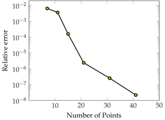
Figure 2: Spectral accuracy of spatial calculation. A sedimenting sphere with $32$ hinged fiber is considered. The abscissa is the number of points per fiber and the ordinate is the error in the velocity of the sphere after moving one radius (about one thousand time steps). As the reference, we used a high-resolution case with $120$ points per fiber.

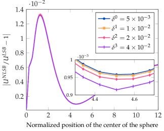
Figure 3: Effect of the regularization factor in $\mathcal{K}_{\delta}$. The relative difference between the computed velocity of a sphere with $32$ attached fibers under a given force using local and nonlocal slender body theories at different values of the regularization parameter $\delta$. The maximum relative error associated with local slender body is $1.4\%$. The inset figure is a closeup of the same figure which shows that the difference between the computed velocities at different $\delta$ decreases with $\delta$. For the two smallest values of $\delta$, this difference is of $\mathcal{O}\left(10^{-5}\right)$ which is within the same range as the residual error for GMRES.

Finally, we explore the effect on the overall dynamics of the regularization factor $\delta$ that appears in the formulation of the non-local self-interaction terms in Eq. 22 . To do so, we use an identical simulation setup as the one used to study the spectral accuracy of the method and compute the transient velocity $U^{NLSB}$ of a sphere with $N_{F}=32$ fibers attached (hinged) to it. For different values of $\delta$ we compare non-local slender body theory (NLSB; Eq. 22) against the local slender body (LSB; dropping the term $\mathcal{K}_{\delta}$), while still taking into account the many-body HIs. In Fig. 3 we plot $\left|U^{NLSB}/U^{LSB}-1\right|$ versus the travel distance of the sphere.

As it is shown, the relative difference between the NLSB and LSB is at most $1.4\%$, indicating that including the non-local self interaction terms has very little effect on the dynamics of the fibers and the attached bodies. The inset plot of Fig. 3 shows a closeup of the figure around $4.5r$ traveled distance. As it can be seen, the difference between the computed velocities at different values of $\delta$ decreases (almost linearly) with decreasing $\delta$, which indicates that numerically evaluated $\mathcal{K}_{\delta}[\bm{f}]$ is a smooth function of $\delta$. For the two smallest values of $\delta^{0}=5\times 10^{-3}$ and $\delta^{1}=10^{-2}$ the relative difference in the computed values are of $\mathcal{O}(10^{-5})$. In contrast to [102] where specialized quadratures were used to evaluate this integral, we find that our spectral integration is sufficient for computing $\mathcal{K}_{\delta}[\bm{f}]$ accurately.

4 Computational experiments

In this section we consider three representative experiments. First, we verify the consistency of our numerical framework by studying the effect of confinement on the mobility of a “microtubule aster” [72, 108]. We consider an aster located in the center of a spherical shell. In this simple geometry, in certain parameter ranges, the aster can be modeled as a porous medium and the hydrodynamic drag coefficients on the body can be computed analytically using the Brinkman model. We show that our numerical results are in excellent agreement with this model. We further demonstrate that the porous medium model has considerable shortcomings as it fails to capture the elastic behavior of the complex when the timescale of imposed force is shorter than the elastic relaxation time of the fibers.

As a primary biophysical application of our framework, we study the effect of confinement on the dynamics of “pronuclear migration” [89]. The precise and timely positioning of the pronuclear complex, and the ensuing mitotic spindle, within cells is necessary for the proper development of eukaryotic organisms [59, 89, 15]. To gain further insight into the mechanics of pronuclear positioning, we consider models of positioning for cells of varying geometries. We study the time-scale required for proper positioning and show it depends sensitively on the choice of model and cell geometry. We also investigate the effect of varying model parameters on the dynamics of migration. These results demonstrate the potential of in silico experimentation to study cases not easily amenable to in vitro or ex vivo experiment, and to complement theoretical and experimental understanding of cellular processes.

To show the more general applicability of our framework, we conclude by studying a cloud of sedimenting fibers. Our simulations reveal that the sedimenting cloud has gross characteristics similar to those of a sedimenting cloud of particles in either the Stokesian or inertial regimes, but with strong internal alignment dynamics.

In all three studies, microtubule (MT) filaments are our model system for semi-flexible fibers. The biophysical and mechanical parameters related to microtubules and their associated molecular motors that are used in simulating these three conditions are listed in Table 3. These values are reproduced from [48, Table 1]. The references related to these measurements are also provided in [48].

Parameter description	Values used in simulations
MT growth velocity ($V_{g}^{0}$)	0.12 $\kern 0.90005pt\text{$\mu$m}\kern 0.90005pt\text{s}^{-1}$
MT shrinkage velocity ($V_{s}$)	0.288 $\kern 0.90005pt\text{$\mu$m}\kern 0.90005pt\text{s}^{-1}$
MT rate of catastrophe ($f_{cat}^{0}$)	0.014 $\kern 0.90005pt\text{s}^{-1}$
MT rate of rescue ($f_{res}$)	0.014 $\kern 0.90005pt\text{s}^{-1}$
MT bending modulus ($E$)	10 $\kern 0.90005pt\text{p}\text{N}\text{m}^{2}$
MT’s stall force for polymerization reaction ($F^{P}_{S}$)	4.4 pN
Cytoplasmic dynein’s stall force ($F^{\mathrm{stall}}$)	1 pN
Viscosity of cytoplasm ($\eta$)	1 Pas
Longest axis of the cell ( $2\times a_{cor}$)	30 $\mu$m
Radius of pronuclear complex ($a_{PNC}$)	5 $\mu$m

Table 3: The biophysical parameters used in our Simulation. These values are taken from [48, Table 1]. The references related to each measurement is also given in that article.

4.1 The effect of confinement on the hydrodynamic mobility of microtubule asters

One of the main structural elements of the cytoskeleton is the microtubule (MT) filament. Some MT assemblies are formed by MTs nucleating from microtubule organizing centers (MTOC) and radially growing out into the cytoplasm. In some organisms, these astral structures can grow to be as large as the outer boundary of the cell. The confining geometry of the cell may increase the force required to move the aster and any attached structures. To study the effects of confinement on aster mobility, we construct a very simple model of it by modeling the MTOC as a solid sphere where MTs of equal length are radially clamped to it.

Figure 4 shows a schematic of this setup, where the entire structure is centered inside a spherical cell with $r_{c}=6r_{m}$ where $r_{m}$ is the radius of the MTOC and $r_{c}$ is the radius of the cell. We apply an external force to the aster and compute the resulting velocity. The ratio of the external force to this velocity is the hydrodynamic drag coefficient at this location.

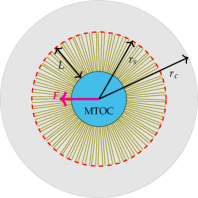
Figure 4: Schematic of Microtubules Aster in Confinement. A schematic presentation of the simulation setup for studying the effect of the cell boundary on the mobility of the microtubule asters. $r_{m}$ denotes the radius of the MTOC (the blue sphere), $r_{c}=6r_{m}$ denotes the cell radius, $L$ is the microtubule length, $r_{s}=r_{m}+L$ is the radius of the astral structure, and $\bm{F}$ is an imposed force.

Aside from direct numerical simulation of the complex, one could attempt to model the astral structure as a porous medium and compute the drag coefficient as a function of its porosity. To verify the physical consistency of our numerical framework, we give an analytical calculation of the drag coefficient by representing the attached fibers as a porous medium where the flow inside the porous domain is modeled using Brinkman equation [8]:

$$\mu\nabla^{2}\bm{u}-\nabla p=\frac{\mu}{\kappa}\left(\bm{u}-\bm{U}_{\mathrm{body}}\right)\mbox{~{}~{}and~{}~{}}\nabla\cdot\bm{u}=0,$$ (72)

where $\bm{u}$ and $\bm{U}_{\mathrm{body}}$ are the velocities of the fluid and the porous domain, respectively. The term $(\mu/\kappa)(\bm{u}-\bm{U}_{\mathrm{body}})$ is the frictional force applied by the porous media on the fluid due to their relative motion, and $\kappa$ is the permeability coefficient that is generally a function of the orientation, aspect ratio, and volume fraction of the fibrous region. It is important to note that the underlying assumption of the Brinkman equation is that the entire porous domain moves as a solid body which in our case is the velocity of the aster. This assumption is not valid in many flow regimes, for example, in the limit of having large enough external force, or velocity fields that deform the MTs causing the MTs to locally have different velocity than the MTOC. If, however, this constraint is met, previous comparisons of simulations based on slender-body theory and boundary integral calculations with Brinkman theory confirm that this model gives an excellent representation of fibrous networks over a wide range of volume fractions [36]. That said, given the geometric structure of an aster array of MTs, a more accurate description would (at the least) use a spatially dependent permeability coefficient. Here for simplicity we make the assumption that we can describe the porous shell through a single constant permeability.

A similar problem in this context has been worked out by [64] where they solved for the flow and the resulting drag coefficient of a sphere with a porous shell that is being pulled in an infinite fluid domain. Here we directly extend their results to a confined flow with a spherical outer boundary. The velocity field in the porous shell $r_{m}<r<r_{s}$ is modeled using the Brinkman equation, Eq. 72, while for $r_{s}<r<r_{c}$ the Stokes equation governs the fluid motion. Flow incompressibility is applied in both regions. The boundary conditions for velocity at $r=r_{m}$ and $r=r_{c}$ are no-slip. On the interface of the porous and fluid, $r=r_{s}$, the boundary conditions are continuity of fluid stress and velocity. For convenience we rewrite the equations in terms of $\tilde{\bm{u}}=\bm{u}-\bm{U}_{\mathrm{body}}$, and represent the velocity in spherical coordinates, $\bm{u}=(u_{r},u_{\theta},u_{\varphi})$. Since the inner sphere is located at the center, the flow is axisymmetric, i.e., $u_{\varphi}=0$ and $\bm{u}(r,\theta)$ with $\theta\in[0,\pi]$. The boundary conditions in this situation simplify to:

$$\left\{\begin{aligned} r&=r_{m}:&\tilde{u}^{B}_{r}(r_{m},\theta)&=0,&\tilde{u}^{B}_{\theta}(r_{m},\theta)&=0,\\ r&=r_{s}:&{\tilde{u}}_{r}^{B}(r_{s},\theta)&={\tilde{u}}_{r}^{F}(r_{s},\theta),&{\tau}_{r\theta}^{B}(r_{s},\theta)&=\tau_{r\theta}^{F}(r_{s},\theta),&p^{B}(r_{s},\theta)&=p^{F}(r_{s},\theta),\\ r&=r_{c}:&\tilde{u}^{F}_{r}(r_{c},\theta)&=-{U}_{\mathrm{body}}\cos(\theta),&\tilde{u}^{F}_{\theta}(r_{c},\theta)&={U}_{\mathrm{body}}\sin(\theta),\\ \end{aligned}\right.$$ (73)

where the $B$ and $F$ superscripts refer to the Brinkman and fluid domains, respectively, and the porous sphere moves in the $\hat{\bm{z}}$ direction, i.e., $\bm{U}_{\mathrm{body}}=U_{\mathrm{body}}\hat{\bm{z}}$. We solve for the flow using the axisymmetric stream function in spherical coordinates subject to the conditions given in Eq. 73. The total force on the porous sphere can be obtained by integrating the stress distribution over the sphere $r=r_{s}$ to find

$$F=2\pi r_{s}^{2}\int_{0}^{\pi}\,\mathrm{d}\theta~{}\Big{[}\tau_{rr}\cos\theta-\tau_{r\theta}\sin\theta\Big{]}_{r=r_{s}}\sin\theta.$$ (74)

We can then analytically compute the drag coefficient.

As the number of MTs increases, the penetration length of the fluid into the porous layer is reduced due to hydrodynamic screening. In the limit of an infinite number of MTs ($\kappa\to 0$) we expect the drag coefficient of the structure to approach the drag coefficient of a sphere with an effective hydrodynamic radius of $r_{s}$. The drag coefficient of a sphere with radius $r_{s}$ centered within a sphere of radius $r_{c}$ is given by [35]:

$$\gamma_{b}=6\pi\eta r_{s}\frac{4(1-\lambda^{5})}{4-9\lambda+10\lambda^{3}-9\lambda^{5}+4\lambda^{6}},\quad\text{where}\,\lambda=\frac{r_{s}}{r_{c}}.$$ (75)

In Fig. 5 we compare the predictions of the Brinkman model for a range of permeabilities from the highly permeable, $\kappa=100$, to nearly impermeable, $\kappa=0.001$, as $r_{s}$ is increased from $2$ to $5$ (recall that $r_{m}=1$ and $r_{c}=6$). The predicted drag coefficients from the Brinkman equation as $\kappa\to 0$ correctly asymptotes to the limit of having a completely impermeable sphere with $r=r_{s}$, given by Eq. 75.

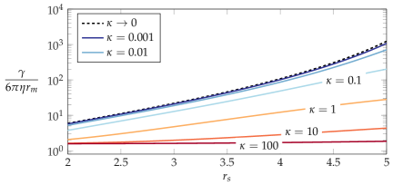
Figure 5: Normalized drag Coefficients of a porous Shell. The predicted drag coefficient based on modeling the porous shell with Brinkman equation compared against the drag coefficient of the completely impermeable case $\kappa\to 0$, computed using Eq. 75.

Next we compare the computed drag coefficient from our direct numerical method against the predictions of the Brinkman equation. To ensure that the flow regime meets the requirements of the Brinkman model and the attached fibers and the aster move as a single body, we chose the external force small enough, $\bm{F}=(1/32)E/L^{2}\hat{\bm{z}}$, to guarantee that the MTs remain nearly straight and that their elastic relaxation time is much shorter than the time required to change the position of the aster more than $1\%$ of its size. As a result, at any given point, the computed drag coefficient represents the instantaneous drag coefficient (if the fiber were assumed completely rigid) with good accuracy. The physical parameters including flexural modulus of fibers and fluid viscosity are chosen from those given in Table 3, and all the lengths are made dimensionless with $a_{PNC}=5\kern 1.00006pt\text{$\mu$m}$, i.e., $L=1$ is equivalent to $5\kern 1.00006pt\text{$\mu$m}$.

Figure 6 shows the computed drag coefficient from our simulation versus the number of the MTs for $N_{F}=32\text{ to }1568$ for three different lengths of the MTs $L=r_{m},2r_{m},3r_{m}$. The drag coefficient is non-dimensionalized by the value of the drag coefficient of an impermeable sphere with radius $r=r_{s}$ from Eq. 75. As expected, the drag coefficient increases with increasing number of fibers. For example, for $r_{s}=2$ the ratio of the drag coefficients at $N_{F}=1568$ to $N_{F}=32$ is $2.22$. This ratio is $4.3$ and $7.52$ for $r_{s}=3$ and $4$, respectively, which shows that the effect of confinement becomes more pronounced with the increase in fiber length, as they get closer to the periphery.

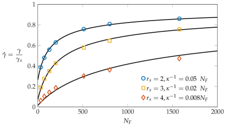
Figure 6: Drag Coefficient vs. Number of MTs. The nondimensional drag coefficient as a function of the number of MTs with $r_{m}=1$, and $r_{c}=6$, and $L/r_{m}=1,2,\text{and }3$. The solid lines present the analytical calculations of the drag coefficient based on Brinkman equation for the porous domain. For each line, the permeability coefficient used in the Brinkman equation is assumed to be inversely dependent on the number of fibers $\kappa^{-1}=cN_{F}$, where the coefficient of proportionality $c$ is computed through regression to the data.

The other important observation is that for a given number of fibers, the longer the length, the farther the drag is from its maximum value corresponding to $\kappa\to 0$ in the theory and $N_{F}\to\infty$ in simulations—compare $\hat{\gamma}/\gamma_{b}=0.86,0.76,\text{and }0.47$ for $L/r_{m}=1,2,\text{and }3$ for $N_{F}=1568$. This is due to the fact that the effective volume fraction of the fibers decreases away from the MTOC as $r^{-2}$ for a given number of attached MTs and therefore the average permeability of the porous domain increases with $L$.

The solid curves in Fig. 6 are the Brinkman predictions for the nondimensional drag coefficient $\hat{\gamma}$ for different MT lengths, as $N_{F}$ is increased. These estimates are in very good agreement with the numerical results (open symbols). A single parameter is fit for each curve. Once the domain of the porous shell is set (i.e., $r_{m,s}$ are chosen), the permeability $\kappa$ must be specified. To remove dependence upon the number of fibers $N_{F}$ we invoke the expected linear scaling of drag forces with volume fraction and take $\kappa^{-1}=cN_{F}$. It is the parameter $c$ that is determined to give the best fit of the Brinkman theory to the simulation results. The fit values of $c$ reduce from $0.05$ for $L=1$, to $0.008$ for $L=3$. This shows that as the length of fibers are increased, the average permeability in the theory increases which is in line with our earlier observation based on numerical simulations.

The Brinkman approach to modeling the interactions of fibrous assemblies with the fluid has substantial limitations. We noted earlier that we are using a constant permeability approximation. Even more notable is that in the Brinkman equations, the response of the porous domain to the fluid is immediate, resulting in a purely viscous response. However, an aster (and many other fibrous structures) are composed of flexible fibers that deform in response to an external force. As a result, the response of the entire system can behave as a viscoelastic material on the time-scales relevant to many cellular processes.

To demonstrate viscoelastic behavior of our model aster and the limitations of Brinkman equation, we consider a setup that is identical to the previous problem except that the external force is now an oscillatory function of time, $F(t)=F_{0}\cos(\omega t)$. We take $L=2r_{m}$, $F_{0}=10E/L^{2}$ and $\omega=a\pi\tau_{E}^{-1}$. Here $\tau_{E}=-\ln(\epsilon^{2}e)E/(8\pi L^{4}\eta)$ is the elastic relaxation time of a single fiber with length $L$ and flexural modulus $E$. For different values of $a$ (0.32, 1.60, 8.00, 40.00, 200.00) we study the response of the aster over many periods of oscillation.

Note that in the range of values of $F_{0}$ and $\omega$ used in our simulations, the oscillation amplitude of the position of the aster is less than $1\%$ of both its radius and the distance between the aster and the cortex. Thus, we can safely assume that variations of the drag coefficient with time are not due to the change in the configuration of the aster with respect to the cell boundary.

In Fig. 7(a) we plot the dimensionless velocity of the aster, $U(t)/U_{0}$, against the dimensionless applied force, $F(t)/F_{0}$, over a temporal period of oscillation (at long times) for different frequencies $\omega$. The velocity is non-dimensionalized by the velocity $U_{0}$ of the spherical core in the absence of MTs and under the same force. The Brinkman predictions are also shown.

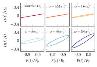
((a))

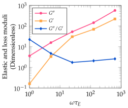
((b))

Figure 7: Viscoelastic behavior of the microtubule asters. LABEL:sub@fig:lissajous The instantaneous velocity of the microtubule aster under an oscillatory force with various frequencies. LABEL:sub@fig:viscoelastic The loss and elastic moduli and their ratio versus frequency computed from the results shown in LABEL:sub@fig:lissajous.

For the Brinkman equation the response is entirely viscous, and so the velocity is completely in phase with the applied force i.e., in the linear response regime ${U(t)}/U_{0}=(\gamma_{0}/\gamma)\cos(\omega t)$, where $\gamma_{0}$ is the drag coefficient of the spherical core in the absence of fibers. Thus, $U(t)/U_{0}$ versus $F(t)/F_{0}$ gives a line with slope $\gamma_{0}/\gamma$. However when fibers are flexible, their shape, and thus their resistance to the flow, evolves with time resulting in both a frequency-dependent drag and a delay in the response of the velocity of the aster with respect to the applied force, i.e., $U(t)/U_{0}=(\gamma_{0}/\gamma)\cos(\omega t+\delta)$. In this definition, $\delta=0$ and $\delta=\pi/2$ correspond to purely viscous and elastic behaviors, respectively. This change in behavior is visualized by the tilted ellipses in the plots of $U(t)/U_{0}$ versus $F(t)/F_{0}$. The area within each ellipse is proportional to the stored elastic energy. If $\delta=0$ the ellipse reduces to a line (zero stored elastic energy), which is the Brinkman result. Our simulations at the two lowest frequencies approach this limit. In this limit, the time-scale of deformation of fibers becomes shorter than the time-scale of oscillation, $\omega^{-1}$. As a result, the dynamics are essentially quasi-static and the behavior is predominantly viscous. As the frequency is increased, these two time-scales become comparable, and the dynamics become viscoelastic and deviates significantly from the Brinkman predictions. For example, the velocity amplitude in simulation at the largest frequency is about $3.6$ times larger than the value predicted by the Brinkman equation.

The dimensionless elastic and loss moduli, $G^{\prime}$ and $G^{\prime\prime}$, respectively, can be computed as $G^{\prime}(\omega)=(\gamma/\gamma_{0})\omega\sin(\delta)$ and $G^{\prime\prime}(\omega)=(\gamma/\gamma_{0})\omega\cos(\delta)$. The computed values of $G^{\prime}(\omega)$, $G^{\prime\prime}(\omega)$, and their ratio are shown Fig. 7(b). The minimum in $G^{\prime\prime}/G^{\prime}$ gives the characteristic frequency $\omega^{*}$ corresponding to the slowest relaxation time $\tau^{*}=1/{\omega^{*}}$ of the aster. For a single fiber $\omega^{*}=\tau_{E}^{-1}$. For the aster, the critical frequency is roughly $\omega^{*}=8\pi\tau_{E}^{-1}$, that is, the aster relaxation time is $8\pi\approx 25$ times smaller than that for an individual fiber. Thus, in addition to changing the drag on the aster, hydrodynamic interactions within the ensemble also give large changes in its relaxation dynamics. To summarize, this simple example clearly shows the viscoelastic nature of a microtubule aster, and demonstrates the shortcomings of Brinkman equation in describing it.

4.2 Pronuclear positioning in complex geometries

The precise positioning of the pronuclear complex (PNC), and of the ensuing mitotic spindle, is indispensable for the proper development of eukaryotic organisms. Positioning of the spindle in the center of the cell produces equally sized daughter cells while asymmetric positioning leads to daughter cells of different sizes which is essential for producing cell diversity [59]. Positioning in organisms with MTOCs is carried out by astral MTs that nucleate from the MTOC and grow into the cytoplasm. Previous studies on such organisms have shown that the interaction of MTs with the cell cortex (the periphery) can be a key factor in defining the position and orientation of the mitotic spindle. For example, experiments in early stages of cell division in the C. elegans embryo have shown that when the cell cortex is deformed from its native elliptical shape to spherical, the mitotic spindle can fail to properly align with the anterior-posterior AP-axis of the cell [80]. Considering that cells evolve through a variety of shapes during development, it is important to identify the relationship between cell shape and spindle positioning.

To study this, [58] molded individual sea urchin eggs into microfabricated chambers of different geometries and so took the shape of the chamber. They analyzed the location and orientation of the nucleus and mitotic spindle throughout the first cell division and found that the nucleus moves to the center of the chamber and aligns along its longest direction. We demonstrate the applicability of our method in studying the effect of confinement on spindle positioning by taking a similar approach and numerically studying the positioning of a model PNC for shapes other than spheres and ellipsoids.

4.2.1.  Stages and mechanisms of pronuclear positioning

We concentrate on positioning of the pronuclear complex in the single-cell C. elegans embryo. After fertilization and the introduction of the male pronucleus, the female pronucleus approaches and fuses with its male counterpart, which has two MTOCs and associated astral MT arrays. Together this ensemble forms the PNC and its motions are associated with its astral MTs. After centering and rotation of the PNC leading to the alignment of the axis between the MTOCs with the AP-axis (the two primary aspects of positioning), the mitotic spindle forms, chromosomes condense, chromatid pairs are formed, chromosomes are divided and pulled to opposite cell sides, and cell division proceeds [15, 89, 59]. Here we only study the positioning of the pronuclear complex prior to the formation of spindle. A schematic representation of the important structural elements involved in PNC positioning, and its important stages, are shown in Fig. 8.

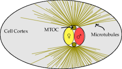
((a)) Key structural elements involved in the PNC migration

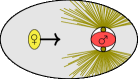
((b)) $t_{(-1)}$, egg fertilization

((c)) $t_{0}$, PNC formation

((d)) $t_{1}$, PNC migration

((e)) $t_{2}$, PNC centering

Figure 8: Schematics of the Pronucleus Complex and stages of PNC migration. LABEL:sub@sfg:schematic-pnc-fert–LABEL:sub@sfg:schematic-pnc-cen The important stages of the migration process in the first cell division of C. elegans embryo. LABEL:sub@sfg:schematic-pnc-fert At $t_{(-1)}$ the egg is fertilized by the male pronucleus and the female pronucleus migrates towards the male pronucleus. LABEL:sub@sfg:schematic-pnc-form At $t_{0}$ the PNC is formed in the posterior side of the cell. This stage is the starting point of our simulations. LABEL:sub@sfg:schematic-pnc-mig Afterwards, from $t_{1}$ to $t_{2}$ the PNC migrates to the center of the cell, while the PNC rotates and the MTOC axis starts to align with the AP-axis. LABEL:sub@sfg:schematic-pnc-cen Finally, at $t_{3}$ the centering and rotation process of the PNC is completed corresponding to the final stage of our simulations.

The force driving PNC positioning is thought to be generated by one, or all, of three potential force-transduction mechanisms operating on astral MTs: cortical pushing, cytoplasmic pulling, or cortical pulling. In the cortical pushing mechanism, pushing forces are applied by MTs growing against the cell cortex [84]. In the cytoplasmic pulling mechanism, MTs are pulled by molecular motors located in the cytoplasm [48, 47]. In both of these proposed mechanisms, the rotation of PNC and its alignment with the AP-axis is achieved by asymmetric ellipsoidal shape of C. elegans embryo [96, 71]. Finally, in the cortical pulling mechanism, MTs are pulled by dyein motors attached to the cortex [28]. The activation of these motors is believed to be regulated by other protein complexes that are distributed asymmetrically throughout the cell boundary, and that because of this asymmetry the details of cell shape may not be crucial to achieving proper positioning [80].

In a concurrent work [71] using the framework presented here, we have studied the positioning of the PNC in the single-cell C. elegans embryo while focusing on the effect of hydrodynamic interaction and the generated cytoplasmic flows in these three mechanisms. For more details the reader is referred to [71]. Here, we instead consider PNC positioning under deformations of the cell shape.

4.2.2.  Biophysical models

We consider simple instantiations of the cortical pushing and cytoplasmic pulling models. Both of these models are generic in the sense that they rely upon rather nonspecific elements of cellular physiology. The cortical pulling model, on the other hand, involves several biophysical elements that are specific to C. elegans [59]. Thus, to keep our study as general as possible with respect to the choice of the organism, we do not consider the cortical pulling here. The general features of that model are discussed in [71]. Below we briefly outline cortical pushing and cytoplasmic pulling models and their implementation within our numerical method. First we begin with a discussion of MT dynamics.

Microtubule polymerization kinetics

Microtubules are polar protein polymers that primarily grow and shrink from their so-called plus-end while the minus-end remains stable. The process of abrupt stochastic transitions between growth and shrinkage is termed dynamic instability [21]. The distribution of MT lengths is determined by their rates of growth $V_{g}$ and shrinkage $V_{s}$, and their frequencies of catastrophe $f_{cat}$ (changing from growing to shrinking), and of rescue $f_{r}$ (changing from shrinking to growing). Previous in vitro measurements and theoretical studies show these rates change under mechanical load [77, 22, 42]. We use an empirical relationship based on the in vitro measurements of [22] to relate the rate of MT growth to an applied compressional load on its plus-end:

$$V_{g}=V_{g}^{0}\exp\left(-\frac{7}{3}\frac{\bm{F}(L)\cdot\bm{X}_{s}}{F_{S}^{P}}\right),$$ (76)

where $V_{g}^{0}$ is the growth rate under no compressive load, $F_{S}^{P}$ is the stall force for MT’s polymerization reaction and $\bm{F}(L)$ is the end-force of the MT. The values used in our simulation for these parameters are listed in Table 3.

The in vitro measurements of [42] suggest that the turnover time from growth to shrinkage, $\tau_{cat}=1/f_{cat}$, of MTs under compressive plus-end-loading is proportional to its growth velocity (itself modulated by the end-force), while other in vivo observations suggest that the turnover time of MTs touching cortex in C. elegans is $1$ to $2$ seconds [59]. We incorporate these two observations and model the rate of catastrophe as

$$f_{cat}=\max\left(f^{0}_{cat}\frac{V_{g}^{0}}{V_{g}},\frac{1}{\tau_{cat}}\right),$$ (77)

where $f^{0}_{cat}$ is the rate of catastrophe under no compressive end-load and $\tau_{cat}$ is the turnover time. In all simulations presented here, unless specified otherwise, we chose $\tau_{cat}=2\kern 1.00006pt\text{s}$.

The cortical pushing model

The movement of the PNC in the cortical pushing model is achieved by compressive forces being applied from the cortex to MTs growing against it. See the schematic of this model in Fig. 9(a). If these forces are not strong enough to stop the growth process altogether, then newly polymerized MT is pushed out from the wall at the polymerization rate, thus lengthening the MT. In turn, this lengthening either pushes the attached PNC away from the cortex, or it deforms the MT. A rough, but useful, estimate of the likelihood of the deformation of MTs upon reaching the cell boundary can be achieved by comparing the stall force for the growth reaction, $F^{P}_{S}=4.4\kern 1.00006pt\text{p}\text{N}$ [103], to the characteristic force required for buckling, $F_{b}=\pi^{2}E/L^{2}$. In the single cell C. elegans embryo, the average MT length is roughly $10\kern 1.00006pt\text{$\mu$m}$, resulting in $F_{b}/F^{S}_{P}\approx 0.20$ implying that MT interactions with the cortex most likely result in buckling (or bending) rather than the stall of polymerization reaction. As a result, a larger compressive force is applied to the MTOC with shorter average length of anchored MTs, since they both buckle less easily and more directly apply force to the PNC, and are more numerous due to dynamic instability. This results in the PNC being pushed away from the side with shorter MTs, and migration towards the side with longer MTs. The combination of torque and force balance on the PNC eventually determines its position and alignment of the centrosomes with respect to the AP-axis [71].

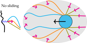
((a)) Cortical Pushing

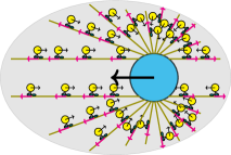
((b)) Cytoplasmic Pulling

Figure 9: Schematics of the biophysical models of PNC migration used in this study. LABEL:sub@sfg:sche-CorPush Cortical pushing model, where compressive forces are applied from the cortex to the MTs growing against it due the polymerization (the forces are modeled as spring forces at the attachment point) LABEL:sub@sfg:sche-CytoPull cytoplasmic pulling model, where the active force for movement is generated by cargo carrying cytoplasmic dynein motors.

In our simulations, we assume that the positions of the growing MTs remain fixed on the periphery once they make contact. We capture this assumption by applying a constraining spring force once an MT plus-end reaches within the critical distance $\Delta r=0.5\kern 1.00006pt\text{$\mu$m}$ from the periphery. The spring force,

$$\bm{F}(L)=-K(\bm{X}(L)-\bm{X}_{att}),$$ (78)

is directed towards the attachment point $\bm{X}_{att}$ and proportional to the distance from it. We set $K=10\kern 1.00006pt\text{p}\text{N}(\text{$\mu$m})^{-1}$. At $0.5\kern 1.00006pt\text{$\mu$m}$ of displacement, this choice of $K$ results in $5\kern 1.00006pt\text{p}\text{N}$ of force, which is bigger than the stall force for polymerization reaction ($F^{P}_{S}=4.4\kern 1.00006pt\text{p}\text{N}$). Thus, the MTs will stop growing prior to reaching to the cell periphery.

We also assume that the attachment to the cortex is a hinged attachment, i.e. the net torque on the growing plus-end is zero. As a result, for growing MTs pushing on the cortex the force $\bm{F}^{ext}$ is given by Eq. 78 and the net torque is zero. When the plus-ends are not at the cortex then the external force and torque on the plus-end are both zero. The minus-end of all MTs are clamped to the MTOC and the boundary conditions are prescribed by Eqs. 36, 37 and 38. The MTs apply a net force and torque to the PNC through their boundary conditions which is computed using Eqs. 64 and 65. Note that in this model there are no active forces from molecular motors on the MTs i.e. $\bm{f}^{E}=0$.

In [71] we use another variation of cortical pushing mechanism where the growing MTs can bend, grow, and slide along the outer boundary. We found that this variation, unlike the one considered here, does not properly align the PNC centrosomes along the AP-axis in physiologically reasonable times, and so do not discuss that variant here.

Cytoplasmic pulling

Cytoplasmic dynein is a minus-end directed molecular motor that attaches and walks along MTs to carry cargo. Through this action, dyneins apply pulling forces on the MTs that are equal in magnitude and opposite in direction to the force they need to exert to drag the cargo through the cytoplasm. Assuming that dynein motors are uniformly distributed in the cytoplasmic volume, the number of motors on MTs increases linearly with their length. As a result, the PNC is pulled in the direction of its longest centrosomal MTs. A schematic of this mechanism is shown in Fig. 9(b). This pulling mechanism can result in the proper centering and alignment of the PNC in computational models of C. elegans embryo [48, 47, 96, 71] that have various degrees of biophysical verisimilitude. In a simple instantiation of this mechanism, we treat the density of the attached dyneins as a continuum field with constant number of attachments per unit length of MT. Thus, the force per unit length, $\bm{f}^{E}_{i}(s)$, and total force, $\bm{F}^{E}_{i}$, applied by cargo-carrying dyneins on the i MT is given by

$$\bm{f}^{E}_{i}(s)=F^{{dyn}}n_{{dyn}}\bm{X}_{i,s}(s),\quad\text{and}\quad\bm{F}^{E}_{i}=\int_{0}^{L}\,\mathrm{d}s~{}f^{E}_{i}(s)=F^{{dyn}}n_{{dyn}}\left[\bm{X}_{i}(L)-\bm{X}_{i}(0)\right],$$ (79)

where $F^{dyn}$ is the magnitude of the force applied from a single motor to an MT, $n_{dyn}$ is the number density of the dyneins per unit length, and $\bm{X}_{i,s}$ is the tangent vector to i MT, where $F^{dyn}$ is related to the walking speed of the motor by a force-velocity relationship as $F=F^{\mathrm{stall}}(1-\max(|V|,V_{max})/V_{max})$, where $F^{\mathrm{stall}}$ is the maximum force applied by the dynein motor on an MT. Moreover, the force and velocity are linearly related through the drag coefficient of the cargo: $F^{dyn}=\gamma V$. If we take the average radius of the cargos as $r_{\mathrm{cargo}}=0.1\kern 1.00006pt\text{$\mu$m}$, and the cytoplasmic viscosity as $\eta=1\kern 1.00006pt\text{P{\kern-0.89996pt}a}\kern 1.00006pt\text{s}$ (see Table 3), we can compute $F^{dyn}$ by combining these two force-velocity relationships which gives $F^{dyn}=0.83F^{\mathrm{stall}}=0.91\kern 1.00006pt\text{p}\text{N}$ [71]. We used $F^{dyn}=0.91\kern 1.00006pt\text{p}\text{N}$ in all the simulations of the cytoplasmic pulling mechanism, presented in this paper.

The boundary conditions on MTs are clamped boundary conditions for the minus-ends, prescribed by Eqs. 36 and 38, and zero force and torque at the plus-end, given by Eq. 35. Also when the MTs reach the periphery (practically, within the small distance $\Delta r$) they instantaneously go through catastrophe. Hence, no pushing forces are applied on the cortex by MTs.

Finally, we note that in both the cytoplasmic and the cortical pushing mechanisms the rotation of PNC and the alignment of the axis of MTOC with the AP-axis is achieved by a symmetry-breaking torque instability that arises from the coupling between the asymmetry of the shape of the cell periphery and the length dependency of the active forces ($\bm{F}^{E}_{i}=F^{dyn}\left[\bm{X}_{i}(L)-\bm{X}_{i}(0)\right]$ and $F_{b}=\pi^{2}E/L^{2}$) [71]. For a spherically shaped eggshell, both models predict centering of the PNC; however MTOC axis will not align with the AP-axis and due to the stochastic nature of the dynamic instability of the microtubules’ polymerization dynamics all the alignment directions are equally sampled over long times.

4.2.3.  Other assumptions and simulation setup

Below we outline other assumptions made in simulating pronuclear migration using both cytoplasmic pulling and cortical pushing models.

Previous studies have shown the nuclear envelope encompassing the nucleus is much stiffer than the plasma membranes of the cell [20]. Based on this and no observations of substantial deformation of the PNC prior to mitosis, we model the PNC as a rigid sphere of radius $a_{PNC}=5\kern 1.00006pt\text{$\mu$m}$ [48]. The mechanics of the cell cortex, however, are in principle more involved. Many important cellular processes, including cytokinesis, cell crawling, and early motion of the female pronucleus towards the male, are achieved by elaborate spatiotemporal deformations of the cell cortex [30]. Nevertheless, the cortex is not known to undergo large distortions during the PNC migration stage. For simplicity then we model the cell cortex as a rigid, fixed surface.

We model the two MTOCs attached to the PNC as two regions set at opposite poles on the spherical PNC surface ($\theta=0,\,\theta=\pi$) defined by the polar angle as $\theta_{1}\leq\pi/5$ and $\theta_{1}\geq 4\pi/5$. We assume that microtubules are mechanically clamped to the PNC and the anchoring sites are uniformly distributed on the MTOC surface area. To obtain a smooth velocity field induced by hydrodynamic interaction of the PNC and the MTs near the anchoring points, we place the anchoring sites slightly away from the surface of the PNC at $1.05a_{PNC}$. Our numerical experiments show that changing this radius in the range of $1.02$ to $1.15$ gives changes in the dynamics that are smaller than the fluctuations in the dynamics due to the stochastic dynamic instability. The same procedure was used for the interaction between MTs and the outer boundary, i.e. the MTs cannot approach closer than $0.95a_{cor}$ to the periphery. Again, changing this distance slightly yielded insignificant changes in the dynamics.

We initialize the simulation by assuming that all MTs start with the same length equal to one-half of PNC radius. The PNC is initially positioned towards the posterior side and, in most simulations, on the AP-axis (denoted here by $\hat{\bm{z}}$). We also performed a number of simulations where the PNC started $0.25a_{PNC}$ away from the AP-axis, and we did not observe any qualitative change in the dynamics or its time-scales. Finally, the axis of MTOCs is set initially at a $90$ degree angle to the AP-axis. This setup approximately replicates the in vivo observations and is consistent with previous modeling efforts [48, 96]. In all simulations we consider $N_{F}=300$ fibers, and discretize each with $N=31$ points except for one set of simulations where $N=51$ was chosen to resolve the large fiber deformations arising in cortical pushing simulations (see Fig. 14(b)).

4.2.4.  Positioning of the PNC in various cell geometries

We represent the shape of the cell periphery in generalized spherical coordinates for an axisymmetric body:

$$x_{cor}=R(\theta)\cos(\varphi)\sin(\theta),\quad y_{cor}=R(\theta)\sin(\varphi)\sin(\theta),\text{ and }\quad z_{cor}=R(\theta)\cos(\theta),$$ (80)

where $\varphi\in[0,2\pi)$, and $\theta\in[0,\pi]$. We consider three different cell shapes, $S_{1,2,3}$, defined by

$$\left\{\begin{aligned} &S_{1}:\quad R_{cor}^{1}(\theta)=a_{cor}\left[1-0.35\cos^{3}\theta-0.15\sin^{3}\theta\right],\\ &S_{2}:\quad R_{cor}^{2}(\theta)=a_{cor}\left[1+0.2\cos(2\theta)-0.2\sin(2\theta)\right],\\ &S_{3}:\quad R_{cor}^{3}(\theta)=a_{cor}\left[1-0.6\sin^{4}\theta\right].\end{aligned}\right.$$ (81)

Here $a_{cor}=25\kern 1.00006pt\text{$\mu$m}$ is chosen in accordance with the longest axis of C. elegans embryo (see Table 3). The corresponding shapes are shown in Fig. 10. In all cases, the $\hat{\bm{z}}$ corresponds to the longest dimension of the cell and its axis of symmetry. In shapes $S_{1}$ and $S_{2}$ the symmetry is only imposed about the $\hat{\bm{z}}$ axis, while shape $S_{3}$ has a mirror symmetry about the $z=0$ plane that cuts through its middle (corresponding to the cell division plane). Also the extent of asymmetry is increased from $S_{1}$ to $S_{2}$. Thus we can simultaneously observe the effect of the type and extent of symmetry on the migration dynamics of the PNC in shapes $S_{1}$, $S_{2}$, and $S_{3}$. These choices of cell confinements in comparison with the typical ellipsoidal shape of the embryos also allow us to study how local deformation of the internal geometry of the cell—by, say, the local contraction of the actin network of the cortex [15]—can affect the dynamics of migration.

A major effect of changing the cell shape is changing the length distribution of MTs within the cell. Since both cortical pushing forces, $\bm{F}(L)$, and cytoplasmic pulling active forces, $\bm{F}^{E}$, depend on the length of the MTs—$\bm{F}(L)\propto L^{-2}$ and $\bm{F}^{E}\propto L$—and average MT length is not well-separated from typical cell sizes, we expect that the variations in the cell shape result in variations in the PNC migration time. Similarly, since asymmetric shape of the cell is a necessary factor in PNC rotation and achieving alignment with the AP-axis in both models, rotation time is also expected to change with the geometry.

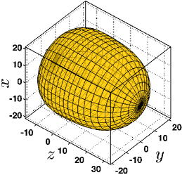
((a)) $S_{1}$

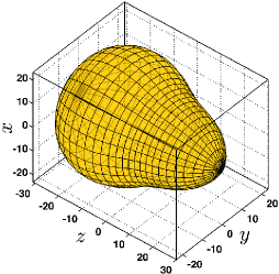
((b)) $S_{2}$

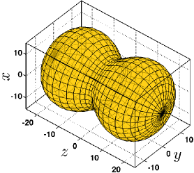
((c)) $S_{3}$

Figure 10: Shapes of cell periphery. Three different shapes of the cell periphery used in this study corresponding to surfaces given by expressions in Eq. 81.

Figures 11, 12 and 13 show snapshots of the PNC and its centrosomal MTs as the structure moves and rotates within the $S_{1}$, $S_{2}$, and $S_{3}$ cell geometries, respectively, for simulations of both the cortical pushing and cytoplasmic pulling models. Also plotted for each case is the temporal evolution of PNC position and the angle $\alpha^{\star}$ between its centrosomal axis (the vector connecting the two MTOC) and the $\hat{\bm{z}}$ axis. The snapshots correspond to different stages in the dynamics: soon after migration begins near the posterior end of cell, after the centering of the PNC, and after the rotation of PNC to its steady-state alignment with the $\hat{\bm{z}}$ axis. We see that the PNC eventually aligns with the $\hat{\bm{z}}$ axis in all three geometries and for both models. The conformation of the MTs is very different between the two models. In the cortical pushing simulations several MTs are strongly buckled due to the compressive forces at the periphery, while in the cytoplasmic pulling simulations MTs are under extensile loads and so remained nearly undeformed.

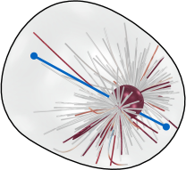
((a)) $t=2\kern 0.90005pt\text{min}$

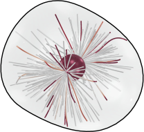
((b)) $t=200\kern 0.90005pt\text{min}$

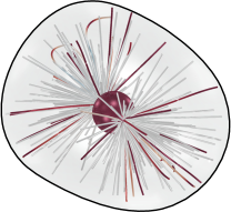
((c)) $t=960\kern 0.90005pt\text{min}$

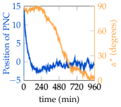
((d))

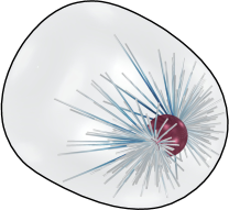
((e)) $t=2\kern 0.90005pt\text{min}$

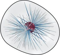
((f)) $t=15\kern 0.90005pt\text{min}$

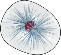
((g)) $t=240\kern 0.90005pt\text{min}$

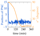
((h))

Figure 11: Snapshots of centering process within $S_{1}$. (a-c) cortical pushing model; (e-g) cytoplasmic pulling model; (d) and (h) the $\hat{\bm{z}}$-component of the position of the PNC and angle between MTOC and the $\hat{\bm{z}}$ axis as a function of time, for cortical pushing and cytoplasmic pulling models respectively. The fibers in all the simulations are colored based on the tension along their length. The colors change from dark red (compressive tension) to dark blue (extensile tension) and the white color denotes no tension. For all the simulations of the PNC migration, $N_{F}=300$. The turnover time in cortical pushing model was taken as $\tau_{cat}=4$ and the number of motors per unit length of the MTs in cytoplasmic model was taken as $n_{dyn}=0.04\kern 0.90005pt(\text{$\mu$m})^{-1}$.

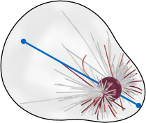
((a)) $t=2\kern 0.90005pt\text{min}$

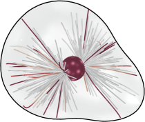
((b)) $t=40\kern 0.90005pt\text{min}$

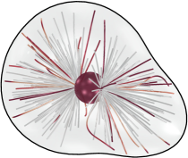
((c)) $t=240\kern 0.90005pt\text{min}$

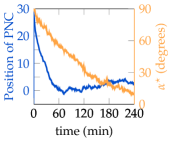
((d))

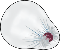
((e)) $t=2\kern 0.90005pt\text{min}$

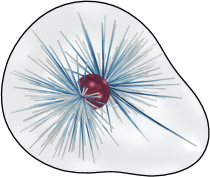
((f)) $t=25\kern 0.90005pt\text{min}$

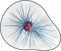
((g)) $t=240\kern 0.90005pt\text{min}$

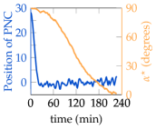
((h))

Figure 12: Snapshots of centering process within $S_{2}$. The descriptions and the parameters used are identical to the one provided in the caption of Fig. 11.

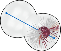
((a)) $t=2\kern 0.90005pt\text{min}$

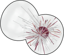
((b)) $t=90\kern 0.90005pt\text{min}$

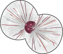
((c)) $t=180\kern 0.90005pt\text{min}$

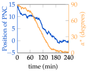
((d))

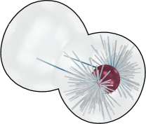
((e)) $t=2\kern 0.90005pt\text{min}$

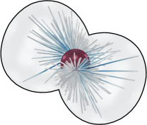
((f)) $t=90\kern 0.90005pt\text{min}$

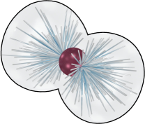
((g)) $t=180\kern 0.90005pt\text{min}$

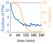
((h))

Figure 13: Snapshots of centering within $S_{3}$. For details refer to the caption of Fig. 11.

The most significant dynamical consequence of changing the cell geometry is the large variation in centering and rotation times between geometries and force-transduction models. For example, in geometry $S_{1}$ the rotation times ($960\kern 1.00006pt\text{min}$, and $150\kern 1.00006pt\text{min}$) are roughly 5 and 10 times larger than the centering time ($200\kern 1.00006pt\text{min}$ and $15\kern 1.00006pt\text{min}$) in the cortical pushing and cytoplasmic pulling simulations, respectively.

In vivo observations of the first cell division in normally-shaped C. elegans embryos, however, show that rotation and positioning occur on the same time-scales [49]. Further, while cytoplasmic pulling and cortical pushing mechanisms do not predict PNC rotation in spherically shaped eggshells, experiments on such geometries show that the PNC can still properly center and align with AP-axis when the embryonic cell is perturbed to be nearly spherical [41, 100]. These observations suggest that other active mechanisms, such as cortical pulling where the necessary asymmetry is not induced by the geometry but by the anisotropic distribution of cortical dyneins on the periphery, can also be involved in pronuclear migration.

Unlike the $S_{1}$ case, the centering and rotation in the cortical pushing model in the $S_{2}$ geometry occurs simultaneously ($240\kern 1.00006pt\text{min}$) while in cytoplasmic pulling model the rotation time ($240\kern 1.00006pt\text{min}$) is again $10$ times larger than the positioning time ($25\kern 1.00006pt\text{min}$). Finally in the $S_{3}$ geometry, centering and rotation happen on the same time-scale ($240\kern 1.00006pt\text{min}$) for both models. The faster rotation of the PNC in case $S_{3}$ may be due to the fact that this is the most anisotropic shape of the geometries.

A few more differences are evident. For example while the steady-state positions of the PNC in the cortical pushing and cytoplasmic pulling models are similar to each other in the $S_{1}$ and $S_{3}$ geometries, the final positions for the two models differ by $5\kern 1.00006pt\text{$\mu$m}$. Another observation is that in the $S_{3}$ cell shape, using the cortical pushing model, the PNC becomes trapped for approximately one-half of the migration time in a dynamically semi-stable position $10\kern 1.00006pt\text{$\mu$m}$ from the center (shown in Fig. 13(b)). Eventually the PNC escapes this dynamical cage as it orients towards the $\hat{\bm{z}}$-axis. To explain this behavior we first note that the $S_{3}$ geometry is roughly two overlapped spheres. The MTs that pass from the posterior sphere to the anterior are long and their associated polymerization forces are weak. Thus, the net cortical pushing force on the PNC, after it reaches to the center of mass of the posterior sphere, is expected to be small. Hence these positions are associated with slower dynamics. In contrast to the cortical pushing model, for the cytoplasmic pulling model the longest MTs that polymerize from posterior to anterior side of the cell induce the largest centering forces. As a result this slower dynamics is not observed in that model (see Fig. 13(h)).

So far, we have only considered the effect of perturbing the cell shape on positioning of the PNC, while biophysical parameters were kept fixed. Although we have chosen the parameters of the model based on experimental measurements, the experimental uncertainties associated with these parameters, including cytoplasmic viscosity, MT polymerization rates, and motor protein densities, are quite significant. Also, many of these parameters—for example the density of the motors—are internally regulated by the cell in different stages of the cell division. Thus, it is important to study how the dynamics change over feasible ranges of the biophysical parameters. To this end, we simulate PNC migration in $S_{1}$ after changing the MT turnover time to $\tau_{cat}=8\kern 1.00006pt\text{s}$ in Eq. 77 for the cortical pushing model, and vary the motor protein density as $n_{dyn}=0.01,0.02,\text{and }0.04\kern 1.00006pt(\text{$\mu$m})^{-1}$ in the cytoplasmic pulling model.

Figure 14 shows snapshots of the conformation of the MTs after the PNC has reached its steady state position in the $S_{1}$ cell geometry for $\tau_{cat}=4\kern 1.00006pt\text{s}$ and $8\kern 1.00006pt\text{s}$. It is clear that the scale of the MT deformations, as well as the number of fibers interacting with the periphery, are significantly larger for simulations with larger turnover times.

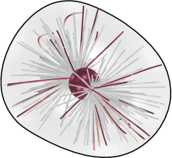
((a)) $\tau_{cat}=4\kern 1.00006pt\text{s}$

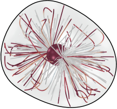
((b)) $\tau_{cat}=8\kern 1.00006pt\text{s}$

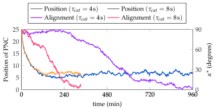
((c)) Positioning and alignment

Figure 14: Centering for different turnover time. Snapshot of the conformation of the MTs after reaching the steady state position and alignment, using turnover times LABEL:sub@sfg:S1_tauvar_1 $\tau_{cat}=4\kern 1.00006pt\text{s}$ (same as Fig. 11) and LABEL:sub@sfg:S1_tauvar_2 $\tau_{cat}=8\kern 1.00006pt\text{s}$ respectively; LABEL:sub@sfg:posangle_tauvar the position and alignment angle of the PNC with respect to time for $\tau_{cat}=4\kern 1.00006pt\text{s}$ and $8\kern 1.00006pt\text{s}$; see Eq. 77.

The centering and rotation dynamics of the PNC for these two turnover times are compared in Fig. 14(c). The main observation is that while increasing $\tau_{cat}$ does not strongly affect the migration dynamics of the PNC, it does strongly affect its rotation; Rotation occurs approximately three times faster for $\tau_{cat}=8\kern 1.00006pt\text{s}$ than for $\tau_{cat}=4\kern 1.00006pt\text{s}$. If the only effect of increasing the turnover time was to increase the average polymerization force from the periphery, we would have expected the translational and rotational motion to be affected similarly. However, this change plainly has a large effect, for example, on the conformation of the centrosomal MTs, and hence on the transmission of the polymerization force to the PNC.

Finally, we study the effect of motor protein density, $n_{dyn}$, on PNC positioning dynamics for the cytoplasmic pulling model in the $S_{1}$ geometry. For this case, Fig. 15 shows the evolution of PNC position and alignment angle for the different values of $n_{dyn}$. The simplest analysis suggests that the speed of PNC migration is proportional to $\bm{F}^{E}$, which would in turn suggest that the time to both translate and rotate to proper position halves with each doubling of $n_{dyn}$. Figure 15(a) clearly shows that the dynamics does not follow this scaling. For of the lowest motor density, $n_{dyn}=0.01$, the PNC monotonically migrates towards its steady-state position and thereafter shows small fluctuations around that position. When the active force is increased by $2$ and $4$ times, the time it takes the PNC to reach its time-averaged steady-state position is reduced by a factor of 3 and 9, respectively. This suggests that the speed of translation has a stronger-than-linear scaling with the active force.

Another interesting effect of increasing motor density is that the PNC starts to oscillate around its mechanical equilibrium position with a well-defined amplitude and frequency. The amplitude of oscillation is greatly increased from $n_{dyn}=0.02$ to $n_{dyn}=0.04$, while the frequency of these oscillations remain roughly unchanged. The source of this rocking motion has similarly been related to enhanced activity of molecular motors in that particular stage with the difference that in this case the motors are bound to the cell cortex [81]. We have formulated a simple mathematical model based on the relative magnitudes of growth and shrinking velocities compared with the velocity of PNC migration to explain these oscillations (to be published elsewhere).

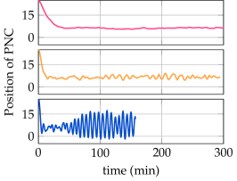
((a))

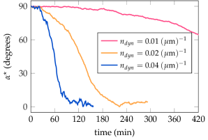
((b))

Figure 15: Position and angle of the PNC for different dynein densities. LABEL:sub@sfg:pulling_osc The $\hat{\bm{z}}$ component of the position of the PNC for three different densities of dynein motors, $n_{dyn}=0.01,\,0.02,\text{and }0.04\kern 1.00006pt(\text{$\mu$m})^{-1}$ LABEL:sub@sfg:pulling_osc_angle the alignment angle of the MTOC axis with respect to the $\hat{\bm{z}}$ axis with respect to time for different density of the motors, $n_{dyn}=0.01,0.02,\text{and }0.04\kern 1.00006pt(\text{$\mu$m})^{-1}$.

The angle between the axis of MTOCs and $\hat{\bm{z}}$ axis at different values of $n_{dyn}$ are plotted in Fig. 15(b). As is seen, the alignment time is greatly reduced when $n_{dyn}$ is increased from $0.01$ to $0.02$ and continues to reduce by roughly a factor of 2 for $n_{dyn}=0.04$. This clearly shows that the rotation time is also not a linear function of the total active force.

In summary we used our numerical platform to study a critical question in the cell division: the effect of confinement geometry and biophysical parameters upon the dynamics of pronuclear migration. We used three different geometries, and two models for the force transduction on MTs required for the positioning of the PNC, i.e., a cortical pushing and the cytoplasmic pulling models. Our results show that the time-scales of positioning and rotation of the PNC can change by several factors depending upon the choice of model. We showed also that varying the biophysical parameters in our force transduction models can change the dynamics tremendously. Finally the steady state orientations and positions of the PNC are in general agreement with the experimental results of [58], for geometries that are qualitatively similar; direct comparison between these two results is not possible since the geometries are not identical. Also the variety of geometries considered in [58] is much large than what we have studied here. A more systematic study of the cell size and shape anisotropy (as is done in [58]) would be an interesting extension of the current study.

4.3 Sedimentation of a cloud of flexible fibers

Due its importance in industrial settings and fundamental studies, the sedimentation of particles in fluids has been a key area of study in suspension mechanics over the past half century. The classical experimental and theoretical literature on sedimentation of spherical particles in viscous fluids is reviewed by [19] and more recently by [29]. There has also been several experimental [38, 37, 60] and numerical [10, 90, 99] studies on sedimentation of suspensions of rigid fibers. Despite its long history and sustained interest, several aspects of sedimenting suspensions remain poorly understood. The origin of many of the complex behaviors has been attributed to the coupling between the long range many-body hydrodynamic interactions and the relative arrangement of the particles, which eventually determines the collective behavior of the suspension [83]. For example, sedimenting fiber suspensions show formation of inhomogeneous clusters of fibers and subsequent enhancement of the sedimentation rate in both numerical and experimental studies [60, 90, 99].

An interesting problem in this context is the sedimentation of a cloud of particles in a viscous fluid. [2] experimentally studied the evolution of a spherically-shaped cloud of a spherical particles. They showed that the cloud undergoes complex deformation as it sediments in the fluid. In a repeating cycle, the initial spherical shape of the cloud deforms to a torus-like shape. The torus structure eventually breaks into smaller clouds which themselves evolve into tori. An extensive overview of this problem and the relevant literature are given in [62, 63]. The majority of research involves studying clouds formed by spherical particles and the effect of shape anisotropy has been studied to a much lesser extent [60, 76]. To the best of our knowledge, sedimentation of flexible fibers has not been studied experimentally and simulation studies are limited to sedimentation of a single semi-flexible fiber [53]. We also note that, recently [66] studied the sedimentation of weakly flexible fiber suspension using particle simulations. In this study the fibers are treated as rigid rods to the leading order and the effect of flexibility only enters through the rate of rotation of the fibers using a continuum theory proposed by the same authors [61].

conclusive study of different aspects of sedimentation of a cloud of flexible fibers is beyond of the scope of this work. Instead, our aim here is to demonstrate that the present numerical framework can be used to investigate some of these aspects by showcasing the dynamics in a limited range of parameter space. We will show that even this limited set of results poses a number of interesting physical questions to be further pursued.

4.3.1.  Background

For simplicity and for consistency with the previous studies, we nondimensionalize velocity and length on the initial velocity and radius of the cloud, respectively. Taking the cloud to be a spherical droplet with effective excess weight of $N_{F}F$ and radius $R_{0}$, the initial velocity of a cloud can be estimated as $V_{c}={N_{F}F}/{(5\pi\mu R_{0})}$ where $N_{F}$ is again the number of fibers, $F$ is the net force acting on each fiber due to their density difference with the fluid.

In dilute suspensions, the flow induced by the sedimenting objects in a Stokesian fluid can be approximated (to the first degree in volume fraction) by representing each object as a point-force within the fluid where the force is the total gravitational force acting on the fiber. Experimental studies on clouds of spherical particles have mostly been limited to the dilute regime ($\phi\leq 0.20$). As a result simulations treating spheres as point-particles have been successful in reproducing many of the observed experimental behavior in these systems [63]. In contrast, for a cloud of fibers the fiber lengths can be comparable to the radius of the cloud itself and the average distance between the fibers may very well be much smaller than their average length, resulting in large effective volume fractions. Thus, reducing the interactions of each fiber with the fluid to a point-force becomes exceedingly inaccurate, and the geometry of individual fibers and their HIs need to be explicitly included. Such differences in geometry and parameter regime, as well as the flexibility of the fibers is likely to result in differences in the evolution of the shape and velocity of a cloud of sedimenting fibers, with respect to clouds of spherical particles.

4.3.2.  Simulation setup

We assume that all fibers have the same length and weight. The boundary conditions for the two ends of fibers are free, and given by relations in Eq. 35. The simulations are initialized by randomly distributing, within an unbounded fluid, the center-of-masses of $N_{F}=1024$ fibers in a spherical volume of radius $R_{0}=1$. Fiber orientations are also taken as random.

For $t>0$ a downwards gravitational load, $\bm{f}^{E}=f_{0}\hat{\bm{z}}$, is applied to all fibers. The simulations are performed for fibers of lengths $L\in\{0.15R_{0},0.25R_{0},0.32R_{0},0.40R_{0}\}$ and aspect ratio of $\epsilon=0.01$.

We define the effective volume fraction of the fibers as

$$\phi^{\star}=\frac{N(L/2)^{3}}{(4/3)\pi R_{0}^{3}}.$$ (82)

The lengths $L=0.15R_{0},0.25R_{0},0.32R_{0},\text{and }0.40R_{0}$ correspond to $\phi^{\star}\approx 0.10,0.50,1.00,\text{and }2.00$. The flexural rigidity of the fibers is chosen to be $E=3.2\times 10^{-3}f_{0}R_{0}^{3}$, which results in very small deformation of fibers in the shortest studied length and moderate deformation for the longest.

4.3.3.  Results

Figure 16 shows snapshots of the evolution of the fiber cloud as it sediments through the fluid.

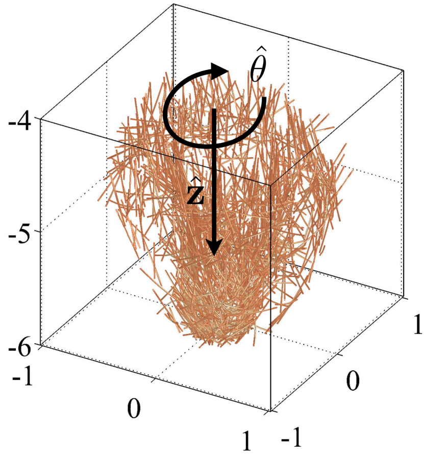
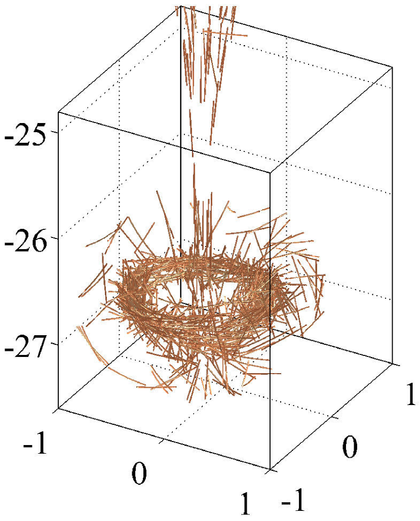
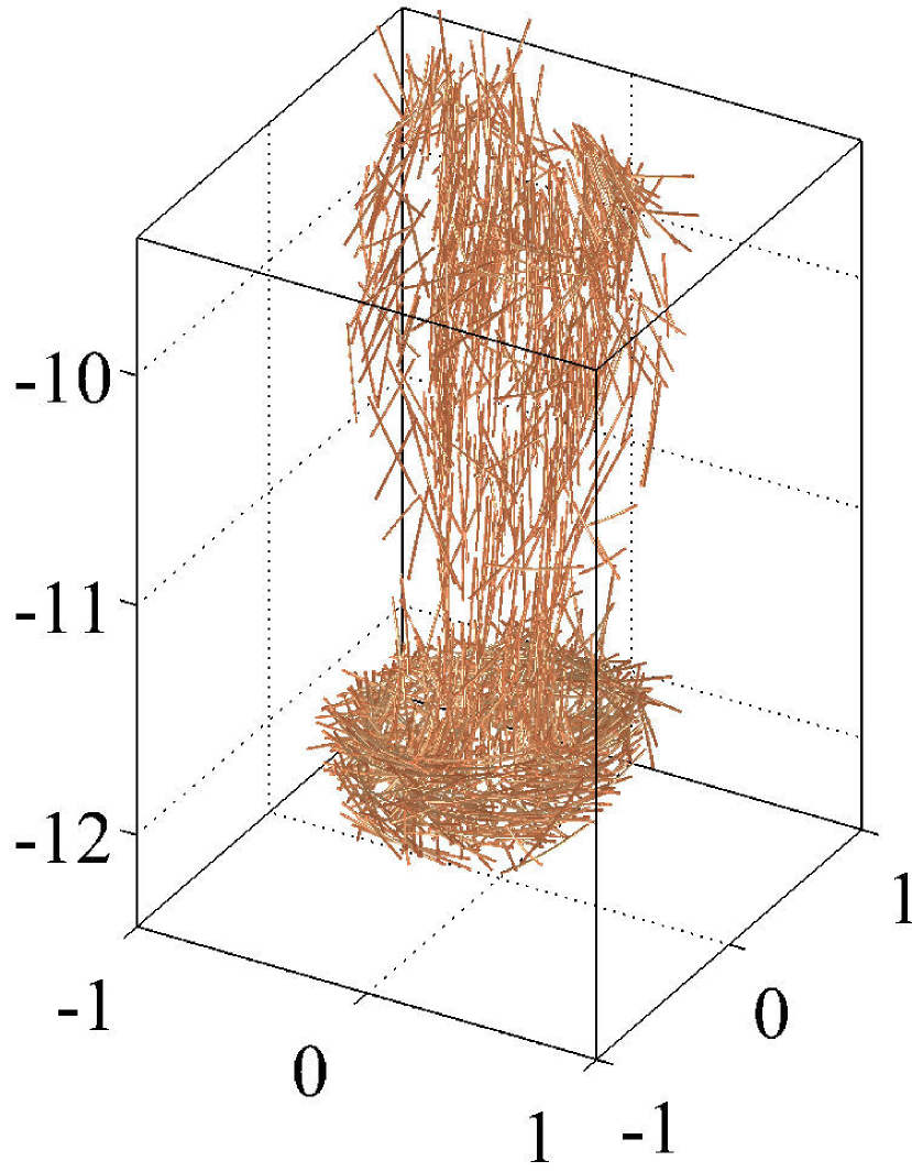
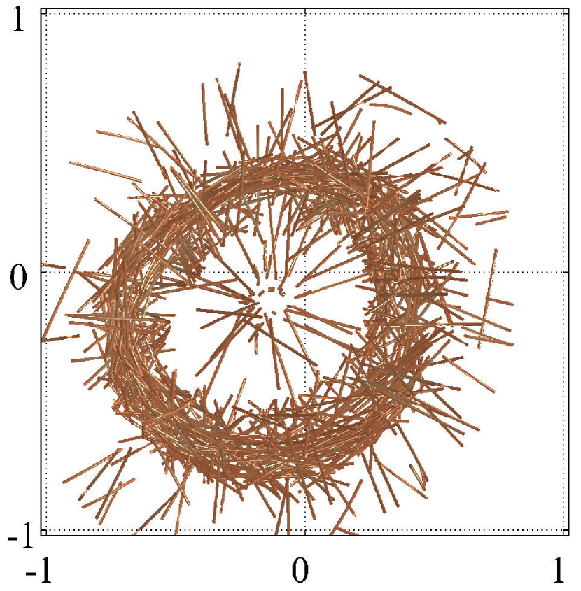
((a)) ((c))          ((b)) ((d))

Figure 16: key Stages in the sedimentation of fibers. Simulation snapshots of the key stages in the shape evolution of the sedimenting cloud of $1024$ flexible fibers with $L/R_{0}=0.32$. LABEL:sub@sfg:sed-init The core of the cloud increases speed and the front of the cloud stretches while the rear contracts. LABEL:sub@sfg:sed-torus A torus-like structure is formed in the front part of the cloud, followed by a trail of fibers in the rear. LABEL:sub@sfg:sed-pinch The torus detaches from the trail. LABEL:sub@sfg:sed-bottom the projection of subfigure LABEL:sub@sfg:sed-pinch in $r{-}\theta$ plane to better depict the organization of the fibers inside the torus ring.

Certain qualitative features are observed for all fiber lengths. In the initial stage of the sedimentation, the fibers align with the $\hat{\bm{z}}$ direction and an inward cusp is observed in the rear face of the cloud, which is shown in Fig. 16(a). Here the rear and front are defined as the parts of the cloud volume with minimum and maximum values of $z$, respectively.

The front face stretching continues until a torus of fibers is formed, trailed by fibers aligned in the sedimentation direction; See Fig. 16(b). The torus diameter then grows in time while the tail of downward aligned fibers gets longer and thinner and eventually pinches off from the torus as is seen in Fig. 16(c). The torus remains stable for up to $150R_{0}$ in sedimentation distance.

These observations are in general agreement with experiments and simulation results of [63] and [76], who studied clouds of spherical particles and rigid fibers. These studies also found that after sedimenting more than $600R_{0}$ the torus structure breaks up into smaller tori. We do not see this in our simulations, most likely due to the shorter simulation times. We find that at sedimentation distances larger than $150R_{0}$, the fibers in the torus become exceedingly close and in near contact and the simulations became numerically unstable. Reducing the time step did not resolve this issue. A similar difficulty was reported by [76] in their simulations of sedimentation of a cloud of rigid fibers. These authors removed this instability by not accounting for HIs between the fibers closer than a cutoff distance. As a result the fibers could pass one another without generating numerical difficulties, though at the unknown cost of not properly accounting for contact mechanics. We did not pursue that route here, and are currently working on including a model for steric interactions between fibers. Another interesting observation is the azimuthal alignment of the fibers within the torus. This is seen in the bottom view of the cloud in Fig. 16(d).

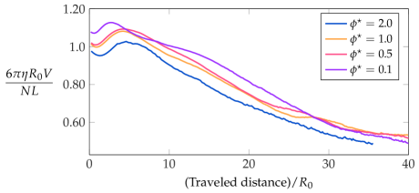
Figure 17: Cloud Sedimentation Velocity. The dimensionless velocity of the cloud versus the sedimentation distance at different volume fractions.

The dimensionless velocity of the cloud as a function of the dimensionless sedimentation distance, for different volume fractions, is given in Fig. 17. The results for different volume fractions all nearly collapse onto a single curve. At all volume fractions, the velocity starts to increase after an initial decrease and then reaches a maximum. The maximum roughly corresponds to the configuration shown in Fig. 16(a). Thereafter, the formation of the tail and the leakage of fibers from the front of the cloud into the tail results in a monotonic decrease of the velocity. This decrease in sedimentation velocity levels off after the torus detaches from the tail in $z/R_{0}>35$, where $z$ is the net displacement of the center of the mass of the cloud since the start of sedimentation.

A key point is that the dimensionless velocity is primarily determined by the cloud’s traveled distance to the initial radius of the cloud, $z/R_{0}$, and is not explicitly a function of time. We also observe that, similar to the sedimentation velocity, the evolution of the shape of the cloud is primarily set by the distance traveled (results not shown here), irrespective of the fibers length and their effective volume fraction.

Next, to gain further insight at a more coarse-grained level, we compute the local number density and the velocity of the fibers. Considering that the structure is statistically symmetric around the direction of gravitational force, $\hat{\bm{z}}$, we use a cylindrical coordinate and average the positions and velocities of the fibers in $\hat{\bm{\theta}}$ direction. We choose center of the coordinate as $(x_{c},y_{c},z_{c})=(0,0,(\max(z)+\min(z))/2)$. Note that the exact value of $z_{c}$ has no effect on the results presented here. Figure 18 illustrates the averaged quantities of interest at the same times shown in Fig. 16LABEL:sub@sfg:sed-init–LABEL:sub@sfg:sed-pinch in the $r{-}z$ plane. The number density is color-coded with white (light) denoting zero and red (dark) denoting the largest number density. The velocity vectors at any given point represent the velocity of the fibers relative to the average sedimentation velocity of the cloud’s center of mass.

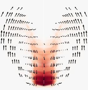
((a))

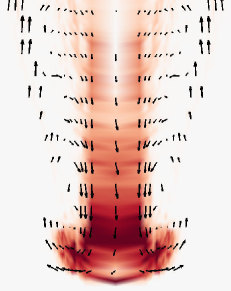
((b))

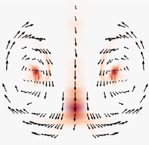
((c))

Figure 18: $\theta$-averaged number density and sedimentation velocity. The number density of the fibers and their relative velocity with respect to the velocity of the center of the cloud, computed by sampling the configuration of the fibers from simulations. The time and physical parameters of the simulations coincide with the ones illustrated in Fig. 16LABEL:sub@sfg:sed-init–LABEL:sub@sfg:sed-pinch. White (light) and red (dark) colors denote low and high volume fractions respectively.

The initial form of the velocity field in Fig. 18 resembles the toroidal flows inside of a sedimenting droplet, which is in line with the previous theoretical work that treats the cloud as a viscous droplet [19]. The flow structure and the concentration variations become more complex in later stages. The velocity field in Fig. 18(c) is reminiscent of the classical flow of a vortex ring at high Reynolds numbers. In fact, [107] reported a similar vortex ring structure for sedimentation of particles in inertially dominant flows, i.e. $Re\gg 1$, where the evolving shape of the cloud is determined by transition from laminar to turbulent flow [107, 11].

Along these lines, [98] theoretically demonstrated that the equations of motion describing the concentration and velocity fluctuations in dilute suspensions of sedimenting non-Brownian particles are analogous to the equations describing turbulent convection at high Prandtl numbers. A more in-depth understanding of this analogy involves studying the dynamics of the sedimenting clouds in the framework of non-equilibrium statistical physics. This typically includes analyzing the correlation functions of number density and velocity as well as their fluctuations in time and space. For the relevant works discussing these aspects, the interested reader is referred to [98, 93, 83, 34, 69].

Finally, for a better understanding of the formation of the azimuthally aligned fibers within the torus, we sample and monitor $q=|\bm{X}_{s}\cdot\hat{\bm{\theta}}|$ in space and time. The definition of $q$ gives zero for the fibers aligned in $r{-}z$ plane and unity for fibers aligned in $\hat{\bm{\theta}}$ direction. The results are shown in Fig. 19. Again, the times coincide with those of Fig. 16.

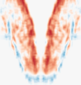
((a))

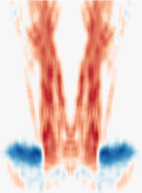
((b))

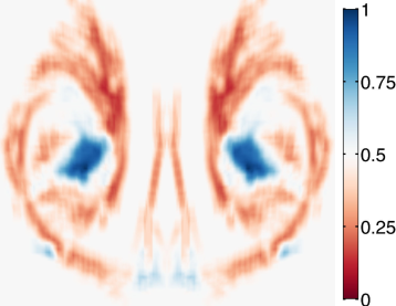
((c))

Figure 19: Alignment of sedimenting fibers. Variations of $q=|\bm{X}_{s}\cdot\hat{\bm{\theta}}|$ in space at the time frames depicted in Fig. 16 and Fig. 18. Recall that $\theta$ is the direction of the symmetry of the shape of the cloud and $\bm{X}_{s}$ is the tangent vector of the fiber at the particular sampling point. The colors change from red denoting the alignment of the tangent (orientation) vector of the fiber in $r{-}z$ plane to blue denoting the alignment in $\hat{\bm{\theta}}$ direction.

As can be seen, at early times the fibers are mostly aligned in $r{-}z$ plane (red color), while a concentration of $\hat{\bm{\theta}}$-aligned fibers are formed in the front region of the cloud (blue color). At later times, these $\hat{\bm{\theta}}$-aligned fibers are migrated to the ring-like structure formed within the torus (see the supplementary material).

For the results presented here, although the longer fibers ($L=0.4R_{0}$) undergo moderate bending, their deformations were not large enough to qualitatively change the overall dynamics and shape of the sedimenting cloud. Another interesting direction of research would be to bridge between the observed dynamics of sedimenting polymeric liquids (very flexible fibers) [88] to the case studied here by systematically varying the flexibility of the fibers and their volume fraction.

5 Conclusions

We presented a platform for the dynamic simulation of semi-flexible fibrous assemblies immersed in a Stokesian fluid with applications to cellular mechanics and suspension mechanics. The hydrodynamic interactions (HIs) of the fibers with the fluid and other bodies are described by the non-local slender body theory while a second-kind boundary integral formulation is used for other rigid bodies and the outer confinement. The deformations of the fibers under external flows and forces are modeled using the Euler–Bernoulli beam theory. We introduced several modifications with respect to the previous numerical treatment of semi-flexible fibers [102], including the spectral representation of the fibers, modeling growth and shrinking dynamics of the fibers (important in biological settings), using fast summation techniques (fast multipole method) for computing HIs, parallelization of the entire computation scheme, and implicit treatment of the HIs of fibers and particles in the time-stepping scheme.

Our numerical tests demonstrate that the method is spectrally accurate in space. Also, due to the use of semi-implicit time-stepping, the number of points per-fiber was found to have no effect on the stable time-step. Finally as a result of the efficient preconditioning of the linear system, GMRES converges to the solution (with relative error of $10^{-5}$) with less than $16$ iterations, for a relatively concentrated assembly of fibers ( $N_{f}=2048$).

We validated our method against the available theoretical and experimental observations in three representative problems. Through this process, we found several new directions of research within each problem that can be pursued using this numerical technique. For example, our simulation technique can be used to investigate the problems that arise in the flow of suspensions in complex geometries, such as shear-induced migration [23, 67, 27] and dynamics of flexible filaments in microfluidic channels [1].

Our method also enables us to compute actively induced cytoplasmic flows in cellular processes. For example, in a concurrent work on the dynamics of pronuclear migration in cell division, we demonstrate that each active mechanism involved in moving the PNC has a distinct flow signature. These generic features of the flow can differentiate between potential active mechanisms. Another important application arises in microrheology measurements, where the motion of a microscopic probe (or probes) is used to infer the rheology of the medium [65, 106, 94]. Within our method it is straightforward to compute the motion of the probe that occurs due to external forcing and the motion of other bodies and a variety of internal active mechanisms. Such fundamental studies can form the basis of microscopically informed coarse-grained theories for describing the mechanics of cytoskeleton.

Our numerical method can be improved in several ways. While thermal fluctuations are typically negligible for microtubule filaments in cytoskeleton, they play a key role in the dynamics of actin and intermediate filaments as well as the dynamics of polymer chains. Thus, to extend the applicability of the platform, thermal fluctuations need to be included and we are currently working on this feature. Steric interactions of fibers were also not imposed in our simulations, and fibers were allowed to cross one another. While this was a very rare event in our simulations, modeling such interactions is required if our framework is to be applied to dense assemblies such as the mitotic spindle structure, dense actin networks, and polymer melts above their entanglement concentration.

In this work, we used the first-order backward Euler method for the time stepping with satisfactory results in terms of accuracy and stability. In modeling of pronuclear migration in Section 4.2, the fibers grow, shrink and alternate between these states, through a Poisson process. As a result, high order backward difference time stepping methods are unnecessarily complex and hinder using adaptive time stepping. High order methods based on spectral deferred correction (SDC) are successfully used for simulation of vesicles in 2D using boundary integral methods with adaptive time stepping [82]. Extension of such method to fiber suspensions is an interesting research direction.

Although several studies demonstrate the importance of HIs in defining the rheology of synthetic systems such as fiber pulps, and the collective dynamics of fibers in cilia and flagellar motion and biofilms [92], these interactions between the fibers in cytoskeletal assemblies have been almost entirely ignored. The typical justification for this was that the long-range HIs beyond the nearest neighbor distance is screened and the dynamics of each individual fiber is dictated by its local interactions with the neighboring fibers [6]. Our example of viscoelastic behavior of a sphere with the shell composed of radial microtubules shows that this picture is not correct in all length scales. We observed that at times longer than the elastic relaxation time of the fibers, the structure can be modeled as a sphere with a porous shell using Brinkman equation. Ignoring the HIs between the MTs would result in a drag coefficient that would linearly increase with the number of fibers, in strong contradictions with the predictions of Brinkman equation and our simulation results. The forced oscillation simulation on the same structure also revealed that the characteristic relaxation time of the porous particle is $25$ times shorter than the relaxation time of individual fibers which shows that many-body HIs substantially modify the elastic properties of the material as well. Thus in attempting to model the HIs through coarse-grained relationships, the underlying assumptions and their correctness in the relevant time- and length-scale must be scrutinized. In this regard, direct simulation provides a powerful tool to inform the reduced models.

References

- AGL+ [11] Nicolas Autrusson, Laura Guglielmini, Sigolene Lecuyer, Roberto Rusconi, and Howard A Stone. The shape of an elastic filament in a two-dimensional corner flow. Physics of Fluids (1994-present), 23(6):063602, 2011.
- AKY [77] K Adachi, S. Kiriyama, and N. Yoshioka. The behavior of a swarm of particles moving in a viscous fluid. Chemical Engineering Science, 33:115–121, 1977.
- ARW [95] UM Ascher, SJ Steven J. SJ Ruuth, and Brian T. R. BTR Wetton. Implicit-Explicit Methods for Time-Dependent Partial Differential Equations. SIAM Journal on Numerical Analysis, 32(3):797–823, June 1995.
- BK [01] Oscar P. Bruno and Leonid A. Kunyansky. A Fast, High-Order Algorithm for the Solution of Surface Scattering Problems: Basic Implementation, Tests, and Applications. Journal of Computational Physics, 169(1):80–110, May 2001.
- BK [06] A. R. Bausch and K. Kroy. A bottom-up approach to cell mechanics. Nature Physics, 2(4):231–238, 2006.
- BM [14] C. P. Broedersz and F. C. MacKintosh. Modeling semiflexible polymer networks. Rev. of Modern Phys., 86(3):995–1036, 2014.
- Boy [01] John P Boyd. Chebyshev and Fourier spectral methods. Courier Corporation, 2001.
- Bri [47] H. C. Brinkman. A calculation of the viscous force exerted by a flowing fluid on a dense swarm of particles. Applied Science Res, A1:27–34, 1947.
- BS [01] Leif E. Becker and Michael J. Shelley. Instability of elastic filaments in shear flow yields first-normal-stress differences. Physical Review Letters, 87(19):198301, 2001.
- BS [02] Jason E Butler and Eric SG Shaqfeh. Dynamic simulations of the inhomogeneous sedimentation of rigid fibres. Journal of Fluid Mechanics, 468:205–237, 2002.
- BTB [03] John W. M. Bush, B. A. Thurber, and F. Blanchette. Particle clouds in homogeneous and stratified environments. Journal of Fluid Mechanics, 489:29–54, 2003.
- BWV [14] Alex Barnett, Bowei Wu, and SK Veerapaneni. Spectrally-accurate quadratures for evaluation of layer potentials close to the boundary for the 2D Stokes and Laplace equations. arXiv preprint arXiv:1410.2187, pages 1–21, 2014.
- BZK [09] David Bommes, Henrik Zimmer, and Leif Kobbelt. Mixed-Integer Quadrangulation. In ACM Transactions On Graphics (TOG), page 77, 2009.
- CFM [05] Ricardo Cortez, Lisa Fauci, and Alexei Medovikov. The method of regularized Stokeslets in three dimensions: Analysis, validation, and application to helical swimming. Physics of Fluids, 17(3):1–14, 2005.
- CH [04] Carrie R Cowan and Anthony a Hyman. Asymmetric cell division in C. elegans: cortical polarity and spindle positioning. Annual review of cell and developmental biology, 20:427–453, 2004.
- Cor [01] Ricardo Cortez. The method of regularized stokeslets. SIAM Journal on Scientific Computing, 23(4):1204–1225, 2001.
- CRZ [15] Eduardo Corona, Abtin Rahimian, and Denis Zorin. A tensor-train accelerated solver for integral equations in complex geometries, 2015.
- CWG [11] Raghunath Chelakkot, Roland G Winkler, and Gerhard Gompper. Semiflexible polymer conformation, distribution and migration in microcapillary flows. Journal of Physics: Condensed Matter, 23(18):184117, 2011.
- DA [85] Robert H Davis and Andreas Acrivos. Sedimentation of noncolloidal particles at low reynolds numbers. Annual Review of Fluid Mechanics, 2(17):91–118, 1985.
- DKWD [04] Kris Noel Dahl, Samuel M Kahn, Katherine L Wilson, and Dennis E Discher. The nuclear envelope lamina network has elasticity and a compressibility limit suggestive of a molecular shock absorber. Journal of cell science, 117(20):4779–4786, 2004.
- DM [97] Arshad Desai and Timothy J Mitchison. Microtubule polymerization dynamics. Annual review of cell and developmental biology, 13(1):83–117, 1997.
- DY [97] M Dogterom and B Yurke. Measurement of the force-velocity relation for growing microtubules. Science, 278(5339):856–860, 1997.
- FAWM [03] Martin Frank, Douglas Anderson, Eric R. Weeks, and Jeffrey F. Morris. Particle migration in pressure-driven flow of a Brownian suspension. J. Fluid Mech., 493:363–378, 2003.
- FLMD+ [05] Heather Flores, Edgar Lobaton, Stefan Méndez-Diez, Svetlana Tlupova, and Ricardo Cortez. A study of bacterial flagellar bundling. Bulletin of mathematical biology, 67(1):137–168, 2005.
- FM [10] Daniel a Fletcher and R Dyche Mullins. Cell mechanics and the cytoskeleton. Nature, 463(7280):485–492, 2010.
- FYJ [15] Szu-Pei Fu, Y.-N. Young, and Shidong Jiang. Efficient brownian dynamics simulation of dna molecules with hydrodynamic interactions in linear flows. Phys. Rev. E, 91:063008, Jun 2015.
- GG [08] C. Gao and J. F. Gilchrist. Shear-induced particle migration in one-, two-, and three-dimensional flows. Phys. Rev. E, 77(2):025301, 2008.
- GGSH [01] S. W. Grill, P. Gönczy, E. H. Stelzer, and A. Hyman. Polarity controls forces governing asymmetric spindle positioning in the Caenorhabditis elegans embryo. Nature, 409(6820):630–633, 2001.
- GH [10] E Lisabeth Guazzelli and John Hinch. Fluctuations and instability in sedimentation. Annual Review of Fluid Mechanics, 2010.
- GK [10] Julia Gilden and Matthew F. Krummel. Control of cortical rigidity by the cytoskeleton: Emerging roles for septins. Cytoskeleton, 67(8):477–486, 2010.
- Göt [00] Thomas Götz. Interactions of fibers and flow: asymptotics, theory and numerics. dissertation., 2000.
- GPW [98] Raymond E. Goldstein, Thomas R. Powers, and Chris H. Wiggins. The Viscous Nonlinear Dynamics of Twist and Writhe. Physical Review Letters, 80(23):9, 1998.
- Gro [12] Robert D Groot. How to impose stick boundary conditions in coarse-grained hydrodynamics of Brownian colloids and semi-flexible fiber rheology. The Journal of chemical physics, 136(6):064901, 2012.
- Gua [01] Elisabeth Guazzelli. Evolution of particle-velocity correlations in sedimentation. Physics of Fluids, 13(6):1537–1540, 2001.
- HB [83] J Happel and H Brenner. Low Reynolds number hydrodynamics, 1965. Martinus Nijhoff Publishers, 1983.
- HF [96] J. J. L. Higdon and G. D. Ford. Permeability of three-dimensional models of fibrous porous media. Journal of Fluid Mechanics, 308(1):341, 1996.
- HG [99] Benjamin Herzhaft and Élisabeth Guazzelli. Experimental study of the sedimentation of dilute and semi-dilute suspensions of fibres. Journal of Fluid Mechanics, 384:133–158, 1999.
- HGMS [96] Benjamin Herzhaft, Élisabeth Guazzelli, Michael B Mackaplow, and Eric SG Shaqfeh. Experimental investigation of the sedimentation of a dilute fiber suspension. Physical review letters, 77(2):290, 1996.
- HO [08] Johan Helsing and Rikard Ojala. On the evaluation of layer potentials close to their sources☆. Journal of Computational Physics, 227(5):2899–2921, February 2008.
- How [01] Jonathon Howard. Mechanics of Motor Proteins and the Cytoskeleton. Sinauer Associates, Inc, first edition, 2001.
- HW [87] Anthony A Hyman and John G White. Determination of cell division axes in the early embryogenesis of caenorhabditis elegans. The J. Cell Biol., 105(5):2123–2135, 1987.
- JDD [03] Marcel E. Janson, Mathilde E. De Dood, and Marileen Dogterom. Dynamic instability of microtubules is regulated by force. Journal of Cell Biology, 161(6):1029–1034, 2003.
- JF [01] C G Joung and X J Fan. Direct simulation of flexible fibers. J. Non-Newtonian Fluid. Mech., 99:1–36, 2001.
- Joh [80] Robert E. Johnson. An improved slender-body theory for Stokes flow. Journal of Fluid Mechanics, 99(02):411, 1980.
- KBGO [13] A. Klöckner, A. H. Barnett, L. Greengard, and M. O’Neil. Quadrature by Expansion: A New Method for the Evaluation of Layer Potentials. Journal of Computational Physics, 0(3):332–349, July 2013.
- KK [89] Seppo J. Karrila and Sangtae Kim. Integral Equations of the Second Kind for Stokes Flow: Direct Solution for Physical Variables and Removal of Inherent Accuracy Limitations. Chemical Engineering Communications, 82(1):123–161, 1989.
- KK [11] Kenji Kimura and Akatsuki Kimura. Intracellular organelles mediate cytoplasmic pulling force for centrosome centration in the Caenorhabditis elegans early embryo. Proceedings of the National Academy of Sciences of the United States of America, 108(1):137–142, 2011.
- KO [05] Akatsuki Kimura and Shuichi Onami. Computer simulations and image processing reveal length-dependent pulling force as the primary mechanism for C. elegans male pronuclear migration. Developmental Cell, 8(5):765–775, 2005.
- KO [07] Akatsuki Kimura and Shuichi Onami. Local cortical pulling-force repression switches centrosomal centration and posterior displacement in C. elegans. Journal of Cell Biology, 179(7):1347–1354, 2007.
- KR [76] JB Keller and SI Rubinow. Slender-body theory for slow viscous flow. Journal of Fluid Mechanics, 75:705–714, 1976.
- Kre [99] Rainer Kress. Linear integral equations, volume 82. Springer-Verlag, New York,, 1999.
- KS [11] Eric E. Keaveny and Michael J. Shelley. Applying a second-kind boundary integral equation for surface tractions in Stokes flow. Journal of Computational Physics, 230(5):2141–2159, March 2011.
- LMSS [13] Lei Li, Harishankar Manikantan, David Saintillan, and Saverio. Spagnolie. The sedimentation of flexible filaments. Journal of Fluid Mechanics, 735:705–736, 2013.
- LP [04] Sookkyung Lim and Charles S. Peskin. Simulations of the Whirling Instability by the Immersed Boundary Method. SIAM Journal on Scientific Computing, 25(6):2066–2083, 2004.
- LS [14] A. Linder and M. Shelley. Elastic fibers in flows. Fluid-Structure Interactions in Low Reynolds Number Flows, edited by C. Duprat and HA Stone (RSC Publishing, 2015), 2014.
- MB [14] Dhairya Malhotra and George Biros. A distributed memory fast multipole method for volume potentials. users.ices.utexas.edu, V(212), 2014.
- MB [15] Dhairya Malhotra and George Biros. PVFMM: A Parallel Kernel Independent FMM for Particle and Volume Potentials. Communications in Computational Physics, 18(03):808–830, 2015.
- MBC [11] Nicolas Minc, David Burgess, and Fred Chang. Influence of cell geometry on division-plane positioning. Cell, 144(3):414–426, 2011.
- McN [13] Francis J. McNally. Mechanisms of spindle positioning. Journal of Cell Biology, 200(2):131–140, 2013.
- MGB [05] Bloen Metzger, Elisabeth Guazzelli, and Jason E. Butler. Large-scale streamers in the sedimentation of a dilute fiber suspension. Physical Review Letters, 95(16):1–4, 2005.
- MLSS [14] Harishankar Manikantan, Lei Li, Saverio E Spagnolie, and David Saintillan. The instability of a sedimenting suspension of weakly flexible fibres. Journal of Fluid Mechanics, 756:935–964, 2014.
- MMNS [01] Gunther Machu, Walter Meile, Ludwig C. Nitsche, and Uwe Schaflinger. Coalescence, torus formation and breakup of sedimenting drops: experiments and computer simulations. Journal of Fluid Mechanics, 447(April 2000):299–336, 2001.
- MNG [07] Bloen Metzger, Maxime Nicolas, and Élisabeth Guazzelli. Falling clouds of particles in viscous fluids. Journal of Fluid Mechanics, 580:283, 2007.
- MNMG [87] Jacob H. Masliyah, Graham Neale, K. Malysa, and Theodorus G.M. Van De Ven. Creeping flow over a composite sphere: Solid core with porous shell. Chemical Engineering Science, 42(2):245–253, 1987.
- Mof [09] Mohammad R.K. Mofrad. Rheology of the Cytoskeleton. Ann. Rev. of Fluid Mech., 41:433–453, 2009.
- MS [16] Harishankar Manikantan and David Saintillan. Effect of flexibility on the growth of concentration fluctuations in a suspension of sedimenting fibers: Particle simulations. Physics of Fluids (1994-present), 28(1):013303, 2016.
- MTS [05] T. Moraczewski, H. Y. Tang, and N. C. Shapley. Flow of a concentrated suspension through an abrupt axisymmetric expansion measured by nuclear magnetic resonance imaging. Journal of rheology, 49(6):1409–1428, 2005.
- NF [07] Francois Nedelec and Dietrich Foethke. Collective Langevin dynamics of flexible cytoskeletal fibers. New J. Physics, 9:0–24, 2007.
- NL [05] Nhan-Quyen Nguyen and Anthony J. C. Ladd. Sedimentation of hard-sphere suspensions at low Reynolds number. Journal of Fluid Mechanics, 525:73–104, 2005.
- NM [15] E Nazockdast and Jeffrey F. Morris. Active microrheology of colloidal suspensions: simulation and microstructural theory. Submitted to Journal of Rheology, 2015.
- NRNS [15] Ehssan Nazockdast, Abtin Rahimian, Daniel Needleman, and Michael Shelley. Cytoplasmic flows as signatures for the mechanics of mitotic positioning. Preprint, pages 1–26, 2015.
- NS [01] François Nédélec and Thomas Surrey. Dynamics of microtubule aster formation by motor complexes. Comptes Rendus de l’Académie des Sciences-Series IV-Physics-Astrophysics, 2(6):841–847, 2001.
- OLC [13] Sarah D. Olson, Sookkyung Lim, and Ricardo Cortez. Modeling the dynamics of an elastic rod with intrinsic curvature and twist using a regularized Stokes formulation. Journal of Computational Physics, 238:169–187, 2013.
- OT [14] Rikard Ojala and Anna-Karin Tornberg. An accurate integral equation method for simulating multi-phase Stokes flow. pages 1–22, April 2014.
- PM [87] Henry Power and Guillermo Miranda. Second Kind Integral Equation Formulation of Stokes’ Flows Past a Particle of Arbitrary Shape. SIAM Journal on Applied Mathematics, 47(4):689, 1987.
- PMGB [10] Joontaek Park, Bloen Metzger, Élisabeth Guazzelli, and Jason E. Butler. A cloud of rigid fibres sedimenting in a viscous fluid. Journal of Fluid Mechanics, 648:351, 2010.
- POO [93] C. S. Peskin, G. M. Odell, and G. F. Oster. Cellular motions and thermal fluctuations: the brownian ratchet. Biophysical journal, 65(1):316, 1993.
- Poz [92] C Pozrikidis. Boundary Integral and Singularity Methods for Linearized Viscous Flow. Cambridge University Press, Cambridge, 1992.
- Poz [01] C Pozrikidis. Interfacial dynamics for Stokes flow. Journal of Computational Physics, 169:250301, 2001.
- PR [08] Dae Hwi Park and Lesilee S. Rose. Dynamic localization of LIN-5 and GPR-1/2 to cortical force generation domains during spindle positioning. Developmental Biology, 315(1):42–54, 2008.
- PRH+ [06] Jacques Pecreaux, Jens-christian Ro, Anthony A Hyman, Karsten Kruse, Frank Ju, Stephan W Grill, and Jonathon Howard. Spindle sscillations during asymmetric cell division require a threshold number of active cortical force generators. Current Biology, pages 2111–2122, 2006.
- QB [14] Bryan Quaife and George Biros. High-order adaptive time stepping for vesicle suspensions with viscosity contrast. pages 1–11, 2014.
- Ram [01] Sriram Ramaswamy. Issues in the statistical mechanics of steady sedimentation. Advances in Physics, 50(3):297–341, 2001.
- RGGG [98] Sigrid Reinsch, Pierre Gönczy, P Gonczy, and Pierre Gönczy. Mechanisms of nuclear positioning. Journal of cell science, 2295(6820):2283–2295, August 1998.
- RK [97] Russell F Ross and Daniel J Klingenberg. Dynamic simulation of flexible fibers composed of linked rigid bodies. J. Chem. Phys., 106:2949–2960, 1997.
- RVZB [15] Abtin Rahimian, Shravan K. Veerapaneni, Denis Zorin, and George Biros. Boundary integral method for the flow of vesicles with viscosity contrast in three dimensions. Journal of Computational Physics, 298:766–786, 2015.
- Saa [03] Yousef Saad. Iterative methods for sparse linear systems. Siam, 2003.
- SB [03] Michael C. Sostarecz and Andrew Belmonte. Motion and shape of a viscoelastic drop falling through a viscous fluid. Journal of Fluid Mechanics, 497:235–252, 2003.
- SD [09] Karsten H Siller and Chris Q Doe. Spindle orientation during asymmetric cell division. Nature cell biology, 11(4):365–374, 2009.
- SDS [05] D Saintillan, E Darve, and E S G Shaqfeh. A smooth particle-mesh Ewald algorithm for Stokes suspension simulations: The sedimentation of fibers. Physics of Fluids, 17(3):33301, 2005.
- SG [98] John M Stockie and Sheldon I Green. Simulating the motion of flexible pulp fibres using the immersed boundary method. Journal of Computational Physics, 147(1):147–165, 1998.
- She [16] M. Shelley. The dynamics of microtubule/motor-protein assemblies in biology and physics. Ann. Rev. Fluid Mech., 48(1):null, 2016.
- SLW [01] P N Segré, F Liu, and D A Weitz. An effective gravitational temperature for sedimentation. Nature, 409, 2001.
- SM [10] Todd M. Squires and Thomas G. Mason. Fluid mechanics of microrheology. Ann. Rev. of Fluid Mech., 42:413–438, January 2010.
- Smi [09] D. J. Smith. A boundary element regularized stokeslet method applied to cilia- and flagella-driven flow. Proceedings of the Royal Society of London A: Mathematical, Physical and Engineering Sciences, 465(2112):3605–3626, 2009.
- SMPS [11] Tamar Shinar, Miyeko Mana, Fabio Piano, and Michael J Shelley. A model of cytoplasmically driven microtubule-based motion in the single-celled Caenorhabditis elegans embryo. Proc. Natl. Acad. Sci. USA, 108(26):10508–10513, 2011.
- SU [00] Michael J. Shelley and Tetsuji Ueda. The Stokesian hydrodynamics of flexing, stretching filaments. Physica D: Nonlinear Phenomena, 146(1-4):221–245, 2000.
- TA [99] P Tong and B. J. Ackerson. Analogies between colloidal sedimentation and turbulent convection at high Prandtl numbers. Physical Review E, 58(6):6931–6934, 1999.
- TG [06] Anna-Karin Tornberg and Katarina Gustavsson. A numerical method for simulations of rigid fiber suspensions. Journal of Computational Physics, 215(1):172–196, 2006.
- THD+ [02] Meng-Fu Bryan Tsou, Adam Hayashi, Leah R DeBella, Garth McGrath, and Lesilee S Rose. LET-99 determines spindle position and is asymmetrically enriched in response to PAR polarity cues in C. elegans embryos. Development (Cambridge, England), 129(19):4469–4481, 2002.
- Tre [00] Lloyd N Trefethen. Spectral methods in MATLAB, volume 10. Siam, 2000.
- TS [04] Anna-Karin Tornberg and Michael J. Shelley. Simulating the dynamics and interactions of flexible fibers in Stokes flows. Journal of Computational Physics, 196(1):8–40, May 2004.
- vDTMD [00] G S van Doorn, C Tanase, B M Mulder, and M Dogterom. On the stall force for growing microtubules. European biophysics journal : EBJ, 29(1):2–6, 2000.
- WA [10] Jingshu Wu and Cyrus K. Aidun. A method for direct simulation of flexible fiber suspensions using lattice Boltzmann equation with external boundary force. International Journal of Multiphase Flow, 36(3):202–209, 2010.
- WHD [01] Torsten Wittmann, Anthony Hyman, and Arshad Desai. The spindle : a dynamic assembly of microtubules and motors. Nature Cell Biology, 3:E28–E34, 2001.
- Wir [09] Denis Wirtz. Particle-tracking microrheology of living cells: principles and applications. Ann. Rev. of biophysics, 38:301–326, 2009.
- WN [96] F Wen and A Nacamuli. The effect of the Rayleigh number on a particle cloud. Hydrodynamics, pages 1275–1280, 1996.
- WR [75] Richard C Weisenberg and Arline C Rosenfeld. In vitro polymerization of microtubules into asters and spindles in homogenates of surf clam eggs. The Journal of cell biology, 64(1):146–158, 1975.
- WS [15] Jeffrey K Wiens and John M Stockie. Simulating flexible fiber suspensions using a scalable immersed boundary algorithm. Computer Methods in Applied Mechanics and Engineering, 290:1–18, 2015.
- YBZ [04] Lexing Ying, George Biros, and Denis Zorin. A kernel-independent adaptive fast multipole algorithm in two and three dimensions. Journal of Computational Physics, 196(2):591–626, 2004.
- YBZ [06] Lexing Ying, George Biros, and Denis Zorin. A high-order 3D boundary integral equation solver for elliptic PDEs in smooth domains. Journal of Computational Physics, 219(1):247–275, 2006.
- YM [95] S Yamamoto and T Matsuoka. Dynamic simulation of fiber suspensions in shear flow. J. Chem. Phys., 102:2254–2260, 1995.
- YM [96] S Yamamoto and T Matsuoka. Dynamic simulation of microstructure and rheology of fiber suspensions. Polym. Eng. Sci., 36(19):2396–2403, 1996.
- ZD [00] AZ Zinchenko and RH Davis. An efficient algorithm for hydrodynamical interaction of many deformable drops. Journal of Computational Physics, 157(2):539–587, 2000.