Exponents for the number of pairs of $\alpha$-favorite points of a simple random walk in ${\mathbb{Z}}^{2}$

Abstract.

We investigate a problem suggested by Dembo, Peres, Rosen, and Zeitouni, which states that the growth exponent of favorite points associated with a simple random walk in $\mathbb{Z}^{2}$ coincides, on average and almost surely, with those of late points and high points associated with the discrete Gaussian free field.

1. Introduction, known results, and unsolved problems

In this paper, we study some properties of the local time of a simple random walk, thereby positively resolving a conjecture suggested in [10]. Although this topic has been studied extensively, numerous open problems still exist. Approximately 60 years ago, Erdős and Taylor [16] proposed a problem concerning a simple random walk in $\mathbb{Z}^{2}$: How many times does a simple random walk $(S_{k})_{k=1}^{\infty}$ revisit the most frequently visited site (up to a specific time)? The points that are most often visited in a simple random walk are called favorite points. In [16], it is shown that, for a simple random walk in ${\mathbb{Z}^{2}}$,

$$\frac{1}{4\pi}\leq\liminf_{n\to\infty}\frac{\max_{x\in{\mathbb{Z}}^{2}}K(n,x)}{(\log n)^{2}}\leq\limsup_{n\to\infty}\frac{\max_{x\in{\mathbb{Z}}^{2}}K(n,x)}{(\log n)^{2}}\leq\frac{1}{\pi}\quad\text{a.s.,}$$

where $K(n,x)$ is the number of times the simple random walk visits $x$ up to time $n$, that is, $K(n,x)=\sum_{i=1}^{n}1_{\{S_{i}=x\}}$. Erdős and Taylor conjectured the existence and value of this limit. This problem was solved by Dembo et al. [8] approximately 20 years ago. In fact, they showed that, for a simple random walk in ${\mathbb{Z}^{2}}$,

$$\lim_{n\to\infty}\frac{\max_{x\in{\mathbb{Z}}^{2}}K(\tau_{n},x)}{4(\log n)^{2}}=\lim_{n\to\infty}\frac{\max_{x\in{\mathbb{Z}}^{2}}K(n,x)}{(\log n)^{2}}=\frac{1}{\pi}\quad\text{a.s,}$$

where $\tau_{n}$ is the first time that the simple random walk exits a disc around the origin of radius $n$. In addition, Dembo et al. [8] showed that

(1.1) $$\frac{\log|\Psi_{n}(\alpha)|}{\log n}\to 2(1-\alpha)\quad\text{ as }n\to\infty\quad\text{ a.s.,}$$

where $\Psi_{n}(\alpha)$ is the set of $\alpha$-favorite points defined as

$$\Psi_{n}(\alpha):=\bigg{\{}x\in D(0,n):K(\tau_{n},x)\geq\bigg{\lceil}\frac{4\alpha}{\pi}(\log n)^{2}\bigg{\rceil}\bigg{\}}$$

for $0<\alpha<1$, where $\lceil a\rceil$ is the smallest integer $n$ with $n\geq a$, $D(x,r):=\{y\in\mathbb{Z}^{2}:d(x,y)\leq r\}$, and $d$ is the Euclidean distance. In other words, $\Psi_{n}(\alpha)$ is the set of points whose local time is an $\alpha$-fraction of the favorite point. They derived these results using an innovative application of the second moment method. (Note that Rosen [20] provided another proof of [8].) In addition, Dembo et al. suggested additional open problems concerning favorite points.

Recently, research on the geometric structure of the favorite points of a simple random walk in $\mathbb{Z}^{d}$ has progressed significantly. For example, in [19], it was shown that the favorite point of a simple random walk in $\mathbb{Z}^{d}$ with $d\geq 2$ almost surely does not appear in the inner boundary of the random walk range after a sufficiently large time. Lifshits and Shi [18] verified that the favorite point of a one-dimensional simple random walk tends to be far from the origin, and the number of times a simple random walk revisits the favorite point up to the cover time on a two-dimensional torus has been estimated in [1]. Several open problems concerning favorite points were raised by Erdős and Révész [14, 15] and Shi and Tóth [21], but almost no solutions have been derived for multi-dimensional walks.

In this paper, we focus on $\alpha$-favorite points. We obtain asymptotic formulas for

(1.2) $$|\{(x,x^{\prime})\in\Psi_{n}(\alpha)^{2}:d(x,x^{\prime})\leq n^{\beta}\}|$$

as $n\to\infty$, where $0<\alpha,\beta<1$ and $|A|$ denotes the cardinality of $A$. Asymptotic formulas such as this can help to determine the joint distribution of the long-time behavior of local time scales. In addition, we want to compare the long-time behavior of the local time of a random walk to the values of the discrete Gaussian free field (DGFF). This is inspired by the results presented in [5] and [10], which show that the asymptotic behavior of (1.2) is similar to that of the number of $\alpha$-high points of the DGFF in $V_{n}:=\{1,\ldots,n\}^{2}$ with zero boundary conditions and, for a simple random walk, the number of $\alpha$-late points in $\mathbb{Z}^{2}_{n}(=\mathbb{Z}^{2}/n\mathbb{Z}^{2})$ for $0<\alpha<1$ ($\alpha$-high points and $\alpha$-late points are defined in Section 2).

2. Framework and principal results

For $0<\alpha,\beta<1$ and $\gamma\geq 0$, let

$$F_{h,\beta}(\gamma): =\gamma^{2}(1-\beta)+\frac{h}{\beta}(1-\gamma(1-\beta))^{2},$$

$$\Gamma_{\alpha,\beta}: =\{\gamma\geq 0:2-2\beta-2\alpha F_{0,\beta}(\gamma)\geq 0\}$$

$$=\{\gamma\geq 0:\alpha\gamma^{2}\leq 1\}.$$

The principal results of this paper are as follows.

Theorem 2.1.

For any $0<\alpha,\beta<1$,

$$\lim_{n\to\infty}\frac{\log|\{(x,x^{\prime})\in\Psi_{n}(\alpha)^{2}:d(x,x^{\prime})\leq n^{\beta}\}|}{\log n}=\rho_{2}(\alpha,\beta)\quad\text{a.s.},$$

where

$$\rho_{2}(\alpha,\beta):=2+2\beta-2\alpha\inf_{\gamma\in\Gamma_{\alpha,\beta}}F_{2,\beta}(\gamma)=\begin{cases}2+2\beta-\frac{4\alpha}{2-\beta}&(\beta\leq 2(1-\sqrt{\alpha})),\\ 8(1-\sqrt{\alpha})-4(1-\sqrt{\alpha})^{2}/\beta&(\beta\geq 2(1-\sqrt{\alpha})).\end{cases}$$

Theorem 2.2.

For any $0<\alpha,\beta<1$,

$$\lim_{n\to\infty}\frac{\log E[|\{(x,x^{\prime})\in\Psi_{n}(\alpha)^{2}:d(x,x^{\prime})\leq n^{\beta}\}|]}{\log n}=\hat{\rho}_{2}(\alpha,\beta),$$

where

$$\hat{\rho}_{2}(\alpha,\beta):=\sup_{\beta^{\prime}\leq\beta}\sup_{\gamma\geq 0}\{2+2\beta^{\prime}-2\alpha F_{2,\beta^{\prime}}(\gamma)\}=\begin{cases}2+2\beta-\frac{4\alpha}{2-\beta}&(\beta\leq 2-\sqrt{2\alpha}),\\ 6-4\sqrt{2\alpha}&(\beta\geq 2-\sqrt{2\alpha}).\end{cases}$$

Remark 2.3.

As $\beta\to 0$, we have

$$\frac{\log E|\Psi_{n}(\alpha)|}{\log n}\to 2(1-\alpha)\quad\text{ as }n\to\infty.$$

This limit is the same as in (1.1).

We now present an intuitive explanation of the roles played by the variables $h$ and $\gamma$. We will estimate the probability that specific points are $\alpha$-favorite points conditioned by crossing numbers around these points. Roughly speaking, we will show that the probability can be written as a functional of $F_{h,\beta}(\gamma)$. $\gamma$ is a crossing number parameter, where $\gamma^{2}(1-\beta)$ corresponds to the probability that a simple random walk crosses a particular circle, and $h(1-\gamma(1-\beta))^{2}/\beta$ corresponds to the probability that $h$-tuple points are $\alpha$-favorite points conditioned by their crossing numbers. We will explain why the domain of a function $F_{2,\beta}(\gamma)$ to have $\rho_{2}(\alpha,\beta)$ has to be restricted in $\Gamma_{\alpha,\beta}$ after proving Proposition 6.4 in Section 6.2. See Section $1.2$ in [6] for more details concerning this difference.

We now present the corresponding known results regarding special points of the DGFF in $V_{n}$ and a simple random walk in $\mathbb{Z}^{2}_{n}$. While not directly connected with $\alpha$-favorite points, the results are important. First, we consider $\alpha$-high points of the DGFF in $V_{n}$. Bolthausen et al. [2] showed that in probability

$$\lim_{n\to\infty}\frac{\max_{x\in V_{n}}\phi_{n}(x)}{\log n}=2\sqrt{\frac{2}{\pi}},$$

where $\{\phi_{n}(x)\}_{x\in V_{n}}$ is the DGFF with zero boundary conditions. In what follows, for $0<\alpha<1$, we define the set of $\alpha$-high points of the DGFF as

$$\mathcal{V}_{n}(\alpha):=\bigg{\{}x\in V_{n}:\frac{\phi_{n}(x)^{2}}{2}\geq\bigg{\lceil}\frac{4\alpha}{\pi}(\log n)^{2}\bigg{\rceil}\bigg{\}}.$$

Daviaud [5] showed that if $\Psi_{n}(\alpha)$ in Theorems 2.1 and 2.2 is replaced by $\mathcal{V}_{n}(\alpha)$, the exponent is the same as that of Theorems 2.1 and 2.2. In addition, there are some interesting results concerning the relation between the local time of a random walk and the DGFF. Eisenbaum et al. [13] reported a powerful equivalence law called the “generalized second Ray-Knight theorem”. The relations they obtained between the local time and the DGFF are vital in deriving the principal results presented in this paper. Ding et al. [12] reported a strong correlation between the expected maximum of the DGFF and the expected cover time (see also [11]).

Next, we define the $\alpha$-late points of a simple random walk in $\mathbb{Z}^{2}_{n}$. For a simple random walk in ${\mathbb{Z}^{2}_{n}}$, Dembo et al. [9] showed that, in probability,

$$\lim_{n\to\infty}\frac{\max_{x\in{\mathbb{Z}}^{2}_{n}}T_{x}}{(n\log n)^{2}}=\frac{4}{\pi},$$

where $T_{x}$ is the hitting time of $x$ for a simple random walk in $\mathbb{Z}^{2}_{n}$. Subsequently, for $0<\alpha<1$, we define the set of $\alpha$-late points in $\mathbb{Z}^{2}_{n}$ as

$$\mathcal{L}_{n}(\alpha):=\bigg{\{}x\in{\mathbb{Z}^{2}_{n}}:\frac{T_{x}}{(n\log n)^{2}}\geq\frac{4\alpha}{\pi}\bigg{\}}.$$

Brummelhuis and Hilhorst [3] obtained a result for $\mathcal{L}_{n}(\alpha)$ corresponding to Theorem 2.2, and verified the same formula with $\mathcal{L}_{n}(\alpha)$ in place of $\Psi_{n}(\alpha)$. Similarly, in [10], a result corresponding to Theorem 2.1 was obtained.

Next, we explain our proof. The upper bound in Theorem 2.1 can be proved using the method developed in [7, 10]. In [7], an estimate is derived for the probability that two points in a disk are covered by a random walk under a particular condition on the crossing number between two circles (see Figure 1).

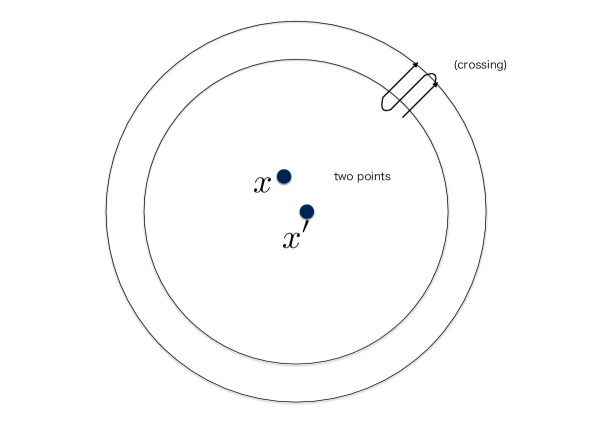
Figure 1.

In [10], this method was used to study late points. In contrast to [7, 10], Proposition 5.1 provides an estimate for the probability that two points in a disk are $\alpha$-favorite points under a particular condition on the crossing number around circles. The result of Proposition 5.1 precisely corresponds to Lemma $6.1$ in [10]. However, the proof of Proposition 5.1 requires an original argument that is different from that of Lemma $6.1$ in [10].

The proof of the lower bound in Theorem 2.1 relies on the second moment method developed in [7, 9, 10]. In the proof of the lower bound in Theorem 2.1, similar to [7, 9, 10], we determine whether a site in $\mathbb{Z}^{2}$ is “successful” or “qualified” in terms of the crossing numbers around that site. However, our definitions of “successful” and “qualified” are slightly different from those of Dembo et al. From the definition of these events, we can compute the number of sites that are successful (or qualified) and use the second moment method. This method produces a variety of limit theorems for functionals of the local time in two dimensions or similar models, as in [7, 9, 10]. At this point, the methods and tools of Belius-Kistler [4] have been surpassed. A new multi-scale refinement of the second moment method is introduced. Roughly speaking, this provides a cleaner analogy between these kinds of problems and branching Brownian motion, and identifies a more natural set of scales (radii of the balls) and a more natural scaling for the excursion counts, showing that their square root can be thought of as a direct equivalent of the path of a particle in branching Brownian motion.

The remainder of this paper is organized as follows. In Section 3.1, we discuss joint distributions of the local time of a general Markov chain, before Section 3.2 discusses some estimates concerning Green’s function. In Section 4, we present the proof of Theorem 2.2. In the proof of Theorem 2.2, we estimate the probability that two points whose distance is specified are $\alpha$-favorite points. To show the lower bound in Theorem 2.2, we use a general Markov chain rule given in Section 3.1. In Section 5, we discuss the key lemma for proving the upper bound in Theorem 2.1, and apply the results in Section 3.1 to estimate the probability conditioned by crossing numbers. In Section 6.1, with the aid of the lemma in Section 5, we prove the upper bound in Theorem 2.1 using an argument similar to that in [10]. In Section 6.2, we prove the lower bound in Theorem 2.1.

3. Preliminary results

3.1. Markov chain argument

In this section, we discuss some preliminary results regarding finite Markov chains, which are used when considering the transitions of a random walk in $\mathbb{Z}^{2}$ from one given set to another. We can reduce such a problem to that for a Markov chain by considering a sequence of hitting times.

Consider a general discrete-time Markov chain $(X_{m})_{m=0}^{\infty}$ on a state space $\{1,2,\ldots,m_{1}+m_{2}+m_{3}\}$. Let $M_{1}:=\{1,\ldots,m_{1}\}$, $M_{2}:=\{m_{1}+1,\ldots,m_{1}+m_{2}\}$ and $M_{3}:=\{m_{1}+m_{2}+1,\ldots,m_{1}+m_{2}+m_{3}\}$. For any $A\subset\{1,2,\ldots,m_{1}+m_{2}+m_{3}\}$, let $T_{A}:=\inf\{m\geq 1:X_{m}\in A\}$. Set

$$g_{i,l}:=P^{i}(\min_{s\in\{1,2,3\}}T_{M_{s}}=T_{M_{l}})$$

for $l\in\{1,2,3\}$ and $i\in\{1,2,\ldots,m_{1}+m_{2}+m_{3}\}$. In addition, for any $j$, $h\in\{1,2,3\}$, let

$$d_{j,h}:=\max_{i\in M_{j}}g_{i,h}.$$

For $i\in\{1,2,\ldots,m_{1}+m_{2}+m_{3}\}$, let $P^{i}$ be the law of $(X_{m})_{m=0}^{\infty}$ starting at $i$. Now, we extend the definition of the local time. We denote the number of visits to a particular set $A\subset\{1,2,\ldots,m_{1}+m_{2}+m_{3}\}$ up to time $n$ by $K(n,A)$, that is, $\sum_{i=1}^{n}1_{\{S_{i}\in A\}}$.

Lemma 3.1.

For any $n_{1}$, $n_{2}\in\mathbb{N}$ and $j\in M_{1}$,

$$P^{j}\bigg{(}K(n_{1}+n_{2},M_{1})=n_{1},K(n_{1}+n_{2},M_{2})=n_{2},X_{n_{1}+n_{2}}\in M_{2}\bigg{)}$$

(3.1) $$\leq\sum_{0\leq i\leq n_{1}\wedge(n_{2}-1)}d_{1,1}^{n_{1}-i}d_{1,2}^{i+1}\begin{pmatrix}n_{1}\\ i\end{pmatrix}d_{2,1}^{i}d_{2,2}^{n_{2}-i-1}\begin{pmatrix}n_{2}-1\\ i\end{pmatrix}$$

and for any $j\in M_{2}$,

$$P^{j}\bigg{(}K(n_{1}+n_{2},M_{1})=n_{1},K(n_{1}+n_{2},M_{2})=n_{2},X_{n_{1}+n_{2}}\in M_{2}\bigg{)}$$

(3.2) $$\leq\sum_{1\leq i\leq n_{1}\wedge n_{2}}d_{1,1}^{n_{1}-i}d_{1,2}^{i}\begin{pmatrix}n_{1}\\ i-1\end{pmatrix}d_{2,1}^{i}d_{2,2}^{n_{2}-i}\begin{pmatrix}n_{2}\\ i\end{pmatrix}$$

where $0!=1$. If $m_{1}=m_{2}=1$, then for any $n_{1}$, $n_{2}\in\mathbb{N}$,

$$P^{1}\bigg{(}K(n_{1}+n_{2},\{1\})=n_{1},K(n_{1}+n_{2},\{2\})=n_{2},X_{n_{1}+n_{2}}=2\bigg{)}$$

(3.3) $$=\sum_{0\leq i\leq n_{1}\wedge(n_{2}-1)}g_{1,1}^{n_{1}-i}g_{1,2}^{i+1}\begin{pmatrix}n_{1}\\ i\end{pmatrix}g_{2,1}^{i}g_{2,2}^{n_{2}-i-1}\begin{pmatrix}n_{2}-1\\ i\end{pmatrix}.$$

• We show that (3.1) holds by induction on $n_{1}+n_{2}$. In the case of $n_{1}=n_{2}=1$, both (3.1) and (3.2) are immediate. Fix $n\geq 2$ and assume that (3.1) and (3.2) hold for any $n_{1}$, $n_{2}\in\mathbb{N}$ with $n_{1}+n_{2}=n$. We want to show (3.1) for any $\tilde{n}_{1}$, $\tilde{n}_{2}\in\mathbb{N}$ with $\tilde{n}_{1}+\tilde{n}_{2}=n+1$. First, we discuss the case in which $\tilde{n}_{2}=1$, and then we discuss the case where $\tilde{n}_{2}\geq 2$. When $\tilde{n}_{2}=1$, for any $j\in M_{1}$,

  $$P^{j}\bigg{(}K(\tilde{n}_{1}+\tilde{n}_{2},M_{1})=\tilde{n}_{1},K(\tilde{n}_{1}+\tilde{n}_{2},M_{2})=\tilde{n}_{2},X_{\tilde{n}_{1}+\tilde{n}_{2}}\in M_{2}\bigg{)}$$

  $$= P^{j}\bigg{(}X_{m}\in M_{1}\text{ for }1\leq m\leq\tilde{n}_{1}+\tilde{n}_{2}-1,X_{\tilde{n}_{1}+\tilde{n}_{2}}\in M_{2}\bigg{)}$$

  $$\leq d_{1,1}^{\tilde{n}_{1}+\tilde{n}_{2}-1}d_{1,2},$$

  and so the claim holds. Next, we discuss the case $\tilde{n}_{2}\geq 2$. The Markov property states that, for any $j\in M_{1}$, $\tilde{n}_{2}\geq 2$, and $\tilde{n}_{1}\in\mathbb{N}$,

  $$P^{j}\bigg{(}K(\tilde{n}_{1}+\tilde{n}_{2},M_{1})=\tilde{n}_{1},K(\tilde{n}_{1}+\tilde{n}_{2},M_{2})=\tilde{n}_{2},X_{\tilde{n}_{1}+\tilde{n}_{2}}\in M_{2}\bigg{)}$$

  $$\leq d_{1,1}\max_{j\in M_{1}}P^{j}\bigg{(}K(\tilde{n}_{1}+\tilde{n}_{2}-1,M_{1})=\tilde{n}_{1}-1,K(\tilde{n}_{1}+\tilde{n}_{2}-1,M_{2})=\tilde{n}_{2},X_{\tilde{n}_{1}+\tilde{n}_{2}-1}\in M_{2}\bigg{)}$$

  $$+d_{1,2}\max_{j\in M_{2}}P^{j}\bigg{(}K(\tilde{n}_{1}+\tilde{n}_{2}-1,M_{1})=\tilde{n}_{1},K(\tilde{n}_{1}+\tilde{n}_{2}-1,M_{2})=\tilde{n}_{2}-1,X_{\tilde{n}_{1}+\tilde{n}_{2}-1}\in M_{2}\bigg{)}$$

  $$\leq d_{1,1}\sum_{0\leq i\leq(\tilde{n}_{1}-1)\wedge(\tilde{n}_{2}-1)}d_{1,1}^{\tilde{n}_{1}-1-i}d_{1,2}^{i+1}\begin{pmatrix}\tilde{n}_{1}-1\\ i\end{pmatrix}d_{2,1}^{i}d_{2,2}^{\tilde{n}_{2}-1-i}\begin{pmatrix}\tilde{n}_{2}-1\\ i\end{pmatrix}$$

  $$+d_{1,2}\sum_{1\leq i\leq\tilde{n}_{1}\wedge(\tilde{n}_{2}-1)}d_{1,1}^{\tilde{n}_{1}-i}d_{1,2}^{i}\begin{pmatrix}\tilde{n}_{1}-1\\ i-1\end{pmatrix}d_{2,1}^{i}d_{2,2}^{\tilde{n}_{2}-1-i}\begin{pmatrix}\tilde{n}_{2}-1\\ i\end{pmatrix}$$

  $$= \sum_{0\leq i\leq\tilde{n}_{1}\wedge(\tilde{n}_{2}-1)}d_{1,1}^{\tilde{n}_{1}-i}d_{1,2}^{i+1}\begin{pmatrix}\tilde{n}_{1}\\ i\end{pmatrix}d_{2,1}^{i}d_{2,2}^{\tilde{n}_{2}-i-1}\begin{pmatrix}\tilde{n}_{2}-1\\ i\end{pmatrix},$$

  where the second inequality comes from the inductive assumptions (3.1) and (3.2). This completes the proof of (3.1). As we can easily obtain (3.2) and (3.3) using the same argument as for (3.1), we omit the proof.

To formulate additional statements, we present the extensional definition of the local time. We denote the number of visits to a particular edge of the vertices $A_{1}$ and $A_{2}\subset\{1,2,\ldots,m_{1}+m_{2}+m_{3}\}$ up to time $n$ by $\tilde{K}(n,A_{1},A_{2})$, that is, $\sum_{i=0}^{n-1}1_{\{S_{i}\in A_{1},S_{i+1}\in A_{2}\}}$. Let $\tilde{M}_{2}:=\{m_{1}+m_{2}+m_{3}+1,\ldots,m_{1}+m_{2}+m_{3}+\tilde{m}_{2}\}$ and consider a Markov chain $(X_{m})_{m=0}^{\infty}$ on a state space $\{1,2,\ldots,m_{1}+m_{2}+m_{3}+\tilde{m}_{2}\}$. Assume that $P^{j}(T_{\tilde{M}_{2}}<T_{M_{1}})=1$ for any $j\in M_{2}$ and $P^{j}(T_{\tilde{M}_{2}}<T_{M_{2}}<T_{M_{3}})=1$ for any $j\in M_{1}$. Let $\tilde{T}_{M_{2}}:=\inf\{m\geq T_{\tilde{M}_{2}}:S_{m}\in M_{2}\}$ and

$$\tilde{d}_{1,1}:= \max_{j\in M_{1}}P^{j}(T_{M_{1}}<T_{M_{2}}),$$

$$\tilde{d}_{1,2}:= \max_{j\in M_{1}}P^{j}(T_{M_{2}}<T_{M_{1}}),$$

$$\tilde{d}_{2,1}:= \max_{j\in M_{2}}P^{j}(T_{\tilde{M}_{2}}<T_{M_{3}},T_{M_{1}}<\tilde{T}_{M_{2}}),$$

$$\tilde{d}_{2,2}:= \max_{j\in M_{2}}P^{j}(T_{\tilde{M}_{2}}<T_{M_{3}},\tilde{T}_{M_{2}}<T_{M_{1}}).$$

Lemma 3.2.

For any $n_{1}$, $n_{2}\in\mathbb{N}$ and for any $j\in M_{1}$,

$$P^{j}\bigg{(}K(T_{M_{3}},M_{1})=n_{1},\tilde{K}(T_{M_{3}},M_{2},\tilde{M}_{2})=n_{2}\bigg{)}$$

(3.4) $$\leq\sum_{0\leq i\leq n_{1}\wedge n_{2}}\tilde{d}_{1,1}^{n_{1}-i}\tilde{d}_{1,2}^{i}\begin{pmatrix}n_{1}\\ i\end{pmatrix}\tilde{d}_{2,1}^{i}\tilde{d}_{2,2}^{n_{2}-i}\begin{pmatrix}n_{2}\\ i\end{pmatrix}$$

and for any $j\in M_{2}$,

$$P^{j}\bigg{(}K(T_{M_{3}},M_{1})=n_{1},\tilde{K}(T_{M_{3}},M_{2},\tilde{M}_{2})=n_{2}\bigg{)}$$

(3.5) $$\leq\sum_{1\leq i\leq n_{1}\wedge n_{2}}\tilde{d}_{1,1}^{n_{1}-i}\tilde{d}_{1,2}^{i}\begin{pmatrix}n_{1}\\ i-1\end{pmatrix}\tilde{d}_{2,1}^{i}\tilde{d}_{2,2}^{n_{2}-i}\begin{pmatrix}n_{2}\\ i\end{pmatrix}.$$

• The proof of the following lemma is almost the same as that of Lemma 3.1, and is therefore omitted. We let $\tilde{d}_{i,l}$ play the role of $d_{i,l}$ in Lemma 3.1. To obtain (3.4), we substitute $n_{2}+1$ for $n_{2}$ in (3.1), and to obtain (3.5), we retain $n_{1}$ and $n_{2}$ in (3.2).

3.2. Hitting probabilities

In this section, we discuss an estimate concerning the hitting probability of a simple random walk in $\mathbb{Z}^{2}$.

First, we compute the probability that the simple random walk does not hit two points until a particular random time. Let $P^{x}$ denote the law of a simple random walk starting at $x$. We simply write $P$ for $P^{0}$. For any $D\subset\mathbb{Z}^{2}$, let $T_{D}:=\inf\{m\geq 1:S_{m}\in D\}$. For simplicity, we write $T_{x_{1},\ldots,x_{j}}$ for $T_{\{x_{1},\ldots,x_{j}\}}$. Given two distinct points $x_{1}$ and $x_{2}$ of $\mathbb{Z}^{2}$ and a nonempty subset of $A\subset\mathbb{Z}^{2}$ that does not contain $\{x_{1},x_{2}\}$, define

$$W_{i,l}:=\sum_{m=0}^{\infty}P^{x_{i}}(S_{m}=x_{l},m<T_{A})$$

for $i,l\in\{1,2\}$.

Lemma 3.3.

For any $i\neq l\in\{1,2\}$ and $A\subset\mathbb{Z}^{2}$,

(3.6) $$P^{x_{i}}(T_{A}<T_{x_{1},x_{2}})=\frac{W_{l,l}-W_{i,l}}{W_{1,1}W_{2,2}-W_{1,2}W_{2,1}}.$$

• Note that $P(T_{A}<\infty)=1$. Then, decomposing all of the events of the simple random walk starting at $x_{i}$ according to the time and the vertex in $\{x_{1},x_{2}\}$ last visited before $T_{A}$ and taking the expectation, we obtain

  $$1=W_{i,1}P^{x_{1}}(T_{A}<T_{x_{1},x_{2}})+W_{i,2}P^{x_{2}}(T_{A}<T_{x_{1},x_{2}}),$$

  for $i\in\{1,2\}$. As $W_{1,2}=P^{x_{1}}(T_{x_{2}}<T_{A})W_{2,2}<W_{2,2}$ and, similarly, $W_{2,1}<W_{1,1}$, we have

  $$W_{1,1}W_{2,2}-W_{1,2}W_{2,1}\neq 0.$$

  Solving the above linear system gives the desired result.

Next, we recall some basic estimates of the hitting probability of a certain circle for a simple random walk in $\mathbb{Z}^{2}$. From [17, Exercise $1.6.8$ or ($4.1$)] and [20, ($4.3$)], we have that, in $0<r<|x|<R$,

$$P^{x}(T_{0}<\tau_{R}) =\frac{\log(R/|x|)+O(|x|^{-1})}{\log R}(1+O((\log|x|)^{-1})),$$

(3.7) $$P^{x}(\tau_{r}<\tau_{R}) =\frac{\log(R/|x|)+O(r^{-1})}{\log(R/{r})},$$

where $\tau_{n}=\inf\{m\geq 0:S_{m}\not\in D(0,n)\}$, as mentioned in Section 1. In addition, by [17, Proposition $1.6.7$] or [20, ($2.2$)], we have that, for any $x\in D(0,n)$,

$$\sum_{m=0}^{\infty}P^{x}(S_{m}=0,m<\tau_{n})=\frac{2}{\pi}\log\bigg{(}\frac{n}{|x|\vee 1}\bigg{)}+O(1).$$

In particular, for $x,y\in D(0,n/3)$,

(3.8) $$G_{n}(x,y)=\frac{2}{\pi}\log\bigg{(}\frac{n}{d(x,y)^{+}}\bigg{)}+O((d(x,y)^{+})^{-1}+n^{-1}+1).$$

Indeed, for $x,y\in D(0,n/3)$,

$$G_{n}(x,y) \leq\sum_{m=0}^{\infty}P^{x-y}(S_{m}=0,m<\tau_{4n/3})$$

$$=\frac{2}{\pi}\log\bigg{(}\frac{n}{d(x,y)^{+}}\bigg{)}+O((d(x,y)^{+})^{-1}+n^{-1}+1),$$

$$G_{n}(x,y) \geq\sum_{m=0}^{\infty}P^{x-y}(S_{m}=0,m<\tau_{2n/3})$$

$$=\frac{2}{\pi}\log\bigg{(}\frac{n}{d(x,y)^{+}}\bigg{)}+O((d(x,y)^{+})^{-1}+n^{-1}+1).$$

Moreover, the Markov property implies that

(3.9) $$P(\tau_{n}<T_{0})=(\sum_{m=0}^{\infty}P(S_{m}=0,m<\tau_{n}))^{-1}=\frac{\pi}{2\log n}(1+o(1)).$$

4. Proof of Theorem 2.2

In this section, we present a proof of Theorem 2.2 by dividing it into lower and upper bounds.

4.1. Proof of the lower bound in Theorem 2.2

First, we discuss the lower bound of Theorem 2.2. To show Theorem 2.2, we introduce the following notation to establish a correspondence with the framework of Section 3.1. Let $\tilde{\alpha}:=\lceil 4\alpha(\log n)^{2}/\pi\rceil$ and $x$, $x^{\prime}$ be two distinct points in $D(0,n)$. Set

$$(U_{0},U_{1},U_{2},U_{3}):=(0,x,x^{\prime},\partial D(0,n))$$

and

$$b_{i,l}:=P^{U_{i}}(\min_{s\in\{1,2,3\}}T_{U_{s}}=T_{U_{l}}),$$

for $i\in\{0,1,2\}$ and $l\in\{1,2,3\}$, where $\partial G:=\{y\in\mathbb{Z}^{2}\setminus G:d(x,y)=1\text{ for some }x\in G\}$ for $G\subset\mathbb{Z}^{2}$. The proof of the lower bound comprises the following two lemmas.

Lemma 4.1.

If we assume $b_{1,1}\leq b_{2,2}$, then

$$P(x,x^{\prime}\in\Psi_{n}(\alpha))\geq\max_{i\in\{1,2\}}b_{0,i}b_{1,2}\frac{1}{\tilde{\alpha}^{2}}P^{x}(T_{x,x^{\prime}}<\tau_{n})^{2\tilde{\alpha}-2}.$$

Lemma 4.2.

Set $s:=\log d(x,x^{\prime})/\log n$. For any $\epsilon>0$, there exists some $c>0$ such that, for all sufficiently large $n\in\mathbb{N}$ and any $x$, $x^{\prime}\in D(0,n^{1-\epsilon})$,

(4.1) $$\max_{i\in\{1,2\}}b_{0,i}\geq c,$$

(4.2) $$b_{1,2}\geq \frac{c}{\log n},$$

(4.3) $$P^{x}(T_{x,x^{\prime}}<\tau_{n})^{2\tilde{\alpha}-2}= \exp\bigg{(}-\frac{\tilde{\alpha}\pi}{(2-s)\log n}+o(1)\log n\bigg{)}.$$

• For $p\geq 2$ and $x\in\mathbb{Z}^{2}$, let

  $$T^{1}_{x}:=\inf\{m\geq 1:S_{m}=x\},\quad T^{p}_{x}:=\inf\{m>T_{x}^{p-1}:S_{m}=x\}.$$

  Note that the time-reversal of a simple random walk yields $b_{1,2}=b_{2,1}$. Then, if we substitute $1$, $2$, $\{3\}$, $n_{1}$, and $n_{2}$ for $x$, $x^{\prime}$, $\partial D(0,n)$, $\tilde{\alpha}-1$, and $\tilde{\alpha}$, (3.3) gives

  $$P(x,x^{\prime}\in\Psi_{n}(\alpha))\geq b_{0,1}P^{x}(x,x^{\prime}\in\Psi_{n}(\alpha),T_{x^{\prime}}^{\tilde{\alpha}}<T_{x}^{\tilde{\alpha}-1})$$

  $$\geq b_{0,1}\times\sum_{0\leq i\leq\tilde{\alpha}-1}b_{1,1}^{\tilde{\alpha}-1-i}b_{1,2}^{i+1}\begin{pmatrix}\tilde{\alpha}-1\\ i\end{pmatrix}b_{2,1}^{i}b_{2,2}^{\tilde{\alpha}-1-i}\begin{pmatrix}\tilde{\alpha}-1\\ i\end{pmatrix}$$

  $$= b_{0,1}b_{1,2}\times\sum_{0\leq i\leq\tilde{\alpha}-1}b_{1,1}^{\tilde{\alpha}-1-i}b_{1,2}^{i}\begin{pmatrix}\tilde{\alpha}-1\\ i\end{pmatrix}b_{2,1}^{i}b_{2,2}^{\tilde{\alpha}-1-i}\begin{pmatrix}\tilde{\alpha}-1\\ i\end{pmatrix}$$

  $$\geq b_{0,1}b_{1,2}\bigg{(}\max_{0\leq i\leq\tilde{\alpha}-1}b_{1,1}^{\tilde{\alpha}-1-i}b_{1,2}^{i}\begin{pmatrix}\tilde{\alpha}-1\\ i\end{pmatrix}\bigg{)}^{2}$$

  $$\geq b_{0,1}b_{1,2}\frac{1}{\tilde{\alpha}^{2}}(b_{1,1}+b_{1,2})^{2\tilde{\alpha}-2}$$

  $$= b_{0,1}b_{1,2}\frac{1}{\tilde{\alpha}^{2}}P^{x}(T_{x,x^{\prime}}<\tau_{n})^{2\tilde{\alpha}-2}$$

  (see Figure 2).

  

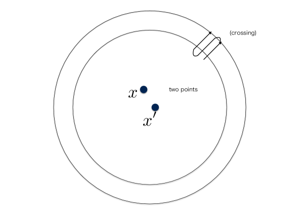
  Figure 2.

  In addition, we also obtain

  $$P(x,x^{\prime}\in\Psi_{n}(\alpha))\geq b_{0,2}P^{x^{\prime}}(x,x^{\prime}\in\Psi_{n}(\alpha),T_{x}^{\tilde{\alpha}}<T_{x^{\prime}}^{\tilde{\alpha}-1})$$

  $$\geq b_{0,2}b_{2,1}\bigg{(}\max_{0\leq i\leq\tilde{\alpha}-1}b_{1,1}^{\tilde{\alpha}-1-i}b_{1,2}^{i}\begin{pmatrix}\tilde{\alpha}-1\\ i\end{pmatrix}\bigg{)}^{2}$$

  $$\geq b_{0,2}b_{1,2}\frac{1}{\tilde{\alpha}^{2}}P^{x}(T_{x,x^{\prime}}<\tau_{n})^{2\tilde{\alpha}-2}.$$

  Thus, we have the desired result.

• First, we show (4.3). Assume $0<\epsilon<1$. Then, by (3.8), we have that

  (4.4) $$\sum_{m=0}^{\infty}P^{U_{i}}(S_{m}\in U_{l},m<\tau_{n})=\begin{cases}\frac{2}{\pi}(1+o(1))\log n&\text{ if }i=l,\\ \frac{2(1-s)}{\pi}(1+o(1))\log n&\text{ if }i\neq l\end{cases}$$

  uniformly in $x$, $x^{\prime}\in D(0,n^{1-\epsilon})$, because $n/n^{1-\epsilon}\geq 3$ for all sufficiently large $n\in\mathbb{N}$. Hence, if we set $T_{A}=\tau_{n}$ in (3.6), then

  (4.5) $$b_{1,3}=\frac{\pi(1+o(1))}{2(2-s)\log n}.$$

  Thus, uniformly in $x$, $x^{\prime}$,

  $$P^{x}(T_{x,x^{\prime}}<\tau_{n})^{2\tilde{\alpha}}= \exp(-2\tilde{\alpha}b_{1,3}+o(1)\log n)$$

  $$= \exp\bigg{(}-\frac{\tilde{\alpha}\pi}{(2-s)\log n}+o(1)\log n\bigg{)}.$$

  Hence, we obtain (4.3). Next, we confirm (4.1) and (4.2). Note that (3.9) yields

  (4.6) $$P^{x}(\tau_{n}<T_{x})=\frac{\pi}{2\log n}(1+o(1))$$

  that uniformly in $x$ and (3.7) implies that, for any $\epsilon>0$, there exists some $c>0$ such that, for all sufficiently large $n\in\mathbb{N}$,

  (4.7) $$P^{x}(T_{x^{\prime}}<\tau_{n})\geq P^{x}(T_{x^{\prime}}<T_{\partial D(x^{\prime},n/2)})\geq\frac{\log(n/2n^{1-\epsilon})}{\log n/2}(1+O((\log n)^{-1}))\geq c,$$

  (4.8) $$P(T_{x}<\tau_{n})=P^{x}(T_{0}<\tau_{n})\geq\frac{\log(n/n^{1-\epsilon})}{\log n}(1+O((\log n)^{-1}))\geq c,$$

  where the equality comes from the time-reversal of a simple random walk. Note that

  $$P^{x}(T_{x^{\prime}}<\tau_{n})=\sum_{i=0}^{\infty}b_{1,1}^{i}b_{1,2}=\frac{1}{1-b_{1,1}}b_{1,2},$$

  and hence, by (4.6) and (4.7), for all sufficiently large $n\in\mathbb{N}$,

  $$b_{1,2}\geq P^{x}(\tau_{n}<T_{x})P^{x}(T_{x^{\prime}}<\tau_{n})\geq\frac{c}{\log n}.$$

  Thus, we obtain (4.2). In addition, by (4.8), we have that there exists some $c>0$ such that, for any $n\in\mathbb{N}$,

  $$\max_{i\in\{1,2\}}b_{0,i}\geq\frac{1}{2}P(T_{x,x^{\prime}}<\tau_{n})\geq\frac{1}{2}P(T_{x}<\tau_{n})\geq c.$$

  Therefore, we obtain (4.1).

• Using Lemmas 4.1 and 4.2, for any $\delta>0$ and $\epsilon>0$, there exists $n_{0}\in\mathbb{N}$ such that, for $n\geq n_{0}$ and $x$, $x^{\prime}\in D(0,n^{1-\epsilon})$,

  (4.9) $$P(x,x^{\prime}\in\Psi_{n}(\alpha))\geq\exp\bigg{(}-\frac{\tilde{\alpha}\pi}{(2-s)\log n}-\delta\log n\bigg{)}.$$

  By (4.9), for any $\delta>0$, $\epsilon>0$, $\beta^{\prime}\in(0,\beta]$, and all sufficiently large $n\in\mathbb{N}$,

  $$E[|\{(x,x^{\prime})\in\Psi_{n}(\alpha)^{2}:d(x,x^{\prime})\leq n^{\beta}\}|]\geq \sum_{\begin{subarray}{c}x,x^{\prime}\in D(0,n^{1-\epsilon}),\\ 0<d(x,x^{\prime})\leq n^{\beta^{\prime}}\end{subarray}}P(x,x^{\prime}\in\Psi_{n}(\alpha))$$

  $$\geq \sum_{\begin{subarray}{c}x,x^{\prime}\in D(0,n^{1-\epsilon}),\\ 0<d(x,x^{\prime})\leq n^{\beta^{\prime}}\end{subarray}}\exp\bigg{(}-\frac{\tilde{\alpha}\pi}{(2-\beta^{\prime})\log n}-\delta\log n\bigg{)}$$

  $$\geq n^{2+2\beta^{\prime}-2\epsilon-4\alpha/(2-\beta^{\prime})-2\delta}.$$

  Note that an elementary calculation yields $\max_{\beta^{\prime}\leq\beta}2+2\beta^{\prime}-4\alpha/(2-\beta^{\prime})=2+2\beta^{\prime}-4\alpha/(2-\beta^{\prime})|_{\beta^{\prime}=\beta\wedge(2-\sqrt{2\alpha})}=\hat{\rho}_{2}(\alpha,\beta)$. Then, as $\delta>0$ and $\epsilon>0$ are arbitrary, we obtain the desired result.

4.2. Proof of the upper bound in Theorem 2.2

We now prove the upper bound in Theorem 2.2. The idea of the upper bound in Theorem 2.2 is similar to that of the lower bound, and we do not require a combinatorial argument in Section 3.1. First, we derive the probability that two particular points are $\alpha$-favorite points.

Lemma 4.3.

For any $\delta>0$, there exists some $n_{0}\in\mathbb{N}$ such that, for any $n\geq n_{0}$ and $x$, $x^{\prime}\in D(0,n)$,

$$P(x,x^{\prime}\in\Psi_{n}(\alpha))\leq\exp\bigg{(}-\frac{\tilde{\alpha}\pi}{(2-s)\log n}+\delta\log n\bigg{)}.$$

• The strong Markov property implies that

  $$P(x,x^{\prime}\in\Psi_{n}(\alpha))$$

  $$\leq P(|\{l<\tau_{n}:S_{l}\in\{x^{\prime},x\}\}|\geq 2\tilde{\alpha})$$

  $$= P(T_{x}<T_{x^{\prime}}\wedge\tau_{n})P^{x}(|\{l<\tau_{n}:S_{l}\in\{x^{\prime},x\}\}|\geq 2\tilde{\alpha}-1)$$

  $$\quad+P(T_{x^{\prime}}<T_{x}\wedge\tau_{n})P^{x^{\prime}}(|\{l<\tau_{n}:S_{l}\in\{x^{\prime},x\}\}|\geq 2\tilde{\alpha}-1)$$

  $$\leq \max_{y\in\{x,x^{\prime}\}}P^{y}(|\{l<\tau_{n}:S_{l}\in\{x^{\prime},x\}\}|\geq 2\tilde{\alpha}-1)$$

  $$\leq \max_{y^{\prime}\in\{x,x^{\prime}\}}P^{y^{\prime}}(T_{x,x^{\prime}}<\tau_{n})\max_{y\in\{x,x^{\prime}\}}P^{y}(|\{l<\tau_{n}:S_{l}\in\{x^{\prime},x\}\}|\geq 2\tilde{\alpha}-2)$$

  $$\leq \cdots$$

  $$\leq \max_{y^{\prime}\in\{x,x^{\prime}\}}P^{y^{\prime}}(T_{x,x^{\prime}}<\tau_{n})^{2\tilde{\alpha}-1}$$

  (4.10) $$\leq \max_{y^{\prime}\in\{x,x^{\prime}\}}P^{y^{\prime}}(T_{x,x^{\prime}}<\tau_{2n})^{2\tilde{\alpha}-1}.$$

  Then, letting $T_{A}=\tau_{2n}$ in (3.6) and using the a similar argument to that for (4.4) and (4.5), we obtain

  $$1-\max_{y^{\prime}\in\{x,x^{\prime}\}}P^{y^{\prime}}(T_{x,x^{\prime}}<\tau_{2n})=\frac{\pi(1+o(1))}{2(2-s)\log n}$$

  uniformly in $x$, $x^{\prime}\in D(0,n)$. Hence, by (4.10), we have the desired result.

• Compared with the lower bound, we need more estimates to bound the summation of $P(x,x^{\prime}\in\Psi_{n}(\alpha))$ in $x^{\prime}\in D(x,n^{\beta})$. We divide the domain of $x^{\prime}$ into $D(x,n^{\beta(1-\alpha)})$ and $D(x,n^{\beta(1-\alpha)})^{c}\cap D(x,n^{\beta})$. We now consider the first case. As $\min\{1/\sqrt{\alpha},2/(2-\beta)\}\geq 1$ with $0<\alpha,\beta<1$ and $F_{2,\beta}(\gamma)$ is decreasing in $\gamma\in[1,(1/\sqrt{\alpha})\wedge(2/(2-\beta))]$,

  (4.11) $$\hat{\rho}_{2}(\alpha,\beta)\geq\rho_{2}(\alpha,\beta)\geq 2+2\beta-2\alpha F_{2,\beta}(1)=2(1-\alpha)+2\beta(1-\alpha).$$

  In addition, (3.9) implies that, for any $\delta>0$, there exists some $n_{0}\in\mathbb{N}$ such that, for any $n\geq n_{0}$,

  $$E[|\Psi_{n}(\alpha)|]= \sum_{x\in D(0,n)}P(x\in\Psi_{n}(\alpha))$$

  $$\leq \sum_{x\in D(0,n)}P^{x}(T_{x}<\tau_{n})^{\tilde{\alpha}-1}$$

  $$\leq \sum_{x\in D(0,n)}P^{x}(T_{x}<T_{\partial D(x,2n)})^{\tilde{\alpha}-1}$$

  (4.12) $$\leq 4n^{2}\times\bigg{(}1-\frac{\pi}{2\log n}+o\bigg{(}\frac{1}{\log n}\bigg{)}\bigg{)}^{\tilde{\alpha}-1}\leq n^{2(1-\alpha)+\delta}.$$

  Using (4.12), we obtain

  $$E[|\{(x,x^{\prime})\in\Psi_{n}(\alpha)^{2}:d(x,x^{\prime})\leq n^{\beta(1-\alpha)}\}|]$$

  (4.13) $$\leq E[|\Psi_{n}(\alpha)|]\times Cn^{2\beta(1-\alpha)}\leq n^{\hat{\rho}_{2}(\alpha,\beta)+\delta},$$

  and hence, we obtain the first case. In addition, using Lemma 4.3, we have that, for any $\delta>0$, $0<h<1$, $\beta^{\prime}\in[\beta(1-\alpha)h^{-1},\beta]$, and all sufficiently large $n\in\mathbb{N}$,

  $$E[|\{(x,x^{\prime})\in\Psi_{n}(\alpha)^{2}:n^{\beta^{\prime}h}<d(x,x^{\prime})\leq n^{\beta^{\prime}}\}|]$$

  $$= \sum_{\begin{subarray}{c}x,x^{\prime}\in D(0,n),\\ n^{\beta^{\prime}h}<d(x,x^{\prime})\leq n^{\beta^{\prime}}\end{subarray}}P(x,x^{\prime}\in\Psi_{n}(\alpha))$$

  $$\leq \sum_{\begin{subarray}{c}x,x^{\prime}\in D(0,n),\\ n^{\beta^{\prime}h}<d(x,x^{\prime})\leq n^{\beta^{\prime}}\end{subarray}}\exp\bigg{(}-\frac{\tilde{\alpha}\pi}{(2-\beta^{\prime}h)\log n}+2\delta\log n\bigg{)}$$

  (4.14) $$\leq n^{2+2\beta^{\prime}-4\alpha/(2-\beta^{\prime}h)+3\delta}.$$

  Note that $\max_{(1-\alpha)\beta\leq\beta^{\prime}\leq\beta}2+2\beta^{\prime}-4\alpha/(2-\beta^{\prime})=\hat{\rho}_{2}(\alpha,\beta)$. Hence, (4.14) yields

  (4.15) $$E[|\{(x,x^{\prime})\in\Psi_{n}(\alpha)^{2}:n^{\beta(1-\alpha)}<d(x,x^{\prime})\leq n^{\beta}\}|]\leq Cn^{\hat{\rho}_{2}(\alpha,\beta)+3\delta}.$$

  Then, because $\delta>0$ and $0<h<1$ are arbitrary, (4.13) and (4.15) produce the desired result.

5. Key lemma for the proof of the upper bound in Theorem 2.1

This section presents large deviation estimates that are the key to the proof of the upper bound in Theorem 2.1. We will estimate the probability of the event that two points are $\alpha$-favorite points conditioned by crossing numbers. Our method involves reducing a simple random walk path to a general Markov chain. This procedure is discussed in Section 3.1.

We now present some definitions. Let $r_{0}:=0$ and $r_{k}:=(k!)^{3}$ for $k\in\mathbb{N}$. Set $K_{n}:=n^{3}r_{n}$ for $n\in\mathbb{N}$ and $f(n,k):=6\alpha(n-k)^{2}\log k$. Now, fix $0<\alpha,\beta<1$. For $z\in D(0,K_{n})$, let $s_{1}:=T_{\partial D(z,r_{k})}$,

$$t_{i} :=\inf\{m>s_{i}:S_{m}\in\partial D(z,r_{k-1})\},$$

$$s_{i+1} :=\inf\{m>t_{i}:S_{m}\in\partial D(z,r_{k})\},$$

and $N_{n,k}^{z}:=\sup\{i\in\mathbb{N}:t_{i}<\tau_{K_{n}}\}$ for $i\geq 1$. That is, $N_{n,k}^{z}$ denotes the number of excursions from $\partial D(z,r_{k})$ to $\partial D(z,r_{k-1})$ up to time $\tau_{K_{n}}$. To state the assertion, we define the domains $\mathbf{Go}^{\beta}$ and $\mathbf{Go}^{h,\beta}$ by

$$\mathbf{Go}^{\beta}: =\{(z,x):z\in D(0,K_{n}),x\in D(z,r_{\beta n-2})\cap D(0,K_{n})\},$$

$$\mathbf{Go}^{h,\beta}: =\{(z,x,x^{\prime}):(z,x),(z,x^{\prime})\in\mathbf{Go}^{\beta},d(x,x^{\prime})\geq r_{\beta hn/2-3}\}.$$

Let $\tilde{\Psi}_{n}(\alpha):=\{x:K(\tau_{n},x)\in[4\alpha/\pi(\log n)^{2},4/\pi(\log n)^{2}]\}$.

Proposition 5.1.

$(1)$ For any $\delta>0$, there exists some $C>0$ such that, for any $\gamma\geq 0$ and $n\in\mathbb{N}$,

(5.1) $$\max_{z\in{\mathbb{Z}}^{2}}P\bigg{(}\frac{N_{n,\beta n}^{z}}{f(n,\beta n)}\geq\gamma^{2}\bigg{)}\leq CK_{n}^{-2\alpha F_{0,\beta}(\gamma)+\delta}.$$

$(2)$ For any $\delta>0$, there exist $C>0$, $\delta_{0}>0$, and $0<h<2$ (with $h$ close to $2$) such that, for any $\gamma\in[0,1/\sqrt{\alpha}]$ and $n\in\mathbb{N}$,

(5.2) $$\max_{(z,x,x^{\prime})\in\mathbf{Go}^{h,\beta}}P\bigg{(}x,x^{\prime}\in\tilde{\Psi}_{K_{n}}(\alpha),\gamma^{2}\leq\frac{N_{n,\beta n}^{z}}{f(n,\beta n)}<(\gamma+\delta_{0})^{2}\bigg{)}\leq CK_{n}^{-2\alpha F_{2,\beta}(\gamma)+\delta}.$$

From (5.2), we obtain the following bound, which we will use in a crucial way.

Corollary 5.2.

For any $\delta>0$, there exist $C>0$ and $\delta_{0}>0$ such that, for any $n\in\mathbb{N}$,

$$\max_{(z,x,x^{\prime})\in\mathbf{Go}^{h,\beta}}P\bigg{(}x,x^{\prime}\in\tilde{\Psi}_{K_{n}}(\alpha),\frac{N_{n,\beta n}^{z}}{f(n,\beta n)}<\bigg{(}\frac{1}{\sqrt{\alpha}}+\delta_{0}\bigg{)}^{2}\bigg{)}\leq CK_{n}^{-2\alpha F_{2,\beta}(\min\{1/\sqrt{\alpha},2/(2-\beta)\})+\delta}.$$

• If we set $C^{\prime}=\lceil 1/(\sqrt{\alpha}\delta_{0})\rceil$, (5.2) implies that

  $$\max_{(z,x,x^{\prime})\in\mathbf{Go}^{h,\beta}}P\bigg{(}x,x^{\prime}\in\tilde{\Psi}_{K_{n}}(\alpha),\frac{N_{n,\beta n}^{z}}{f(n,\beta n)}<\bigg{(}\frac{1}{\sqrt{\alpha}}+\delta_{0}\bigg{)}^{2}\bigg{)}$$

  $$\leq \sum_{k=1}^{C^{\prime}-1}\max_{(z,x,x^{\prime})\in\mathbf{Go}^{h,\beta}}P\bigg{(}x,x^{\prime}\in\tilde{\Psi}_{K_{n}}(\alpha),(k-1)^{2}\delta_{0}^{2}\leq\frac{N_{n,\beta n}^{z}}{f(n,\beta n)}<k^{2}\delta_{0}^{2}\bigg{)}$$

  $$+ \max_{(z,x,x^{\prime})\in\mathbf{Go}^{h,\beta}}P\bigg{(}x,x^{\prime}\in\tilde{\Psi}_{K_{n}}(\alpha),(C^{\prime}-1)^{2}\delta_{0}^{2}\leq\frac{N_{n,\beta n}^{z}}{f(n,\beta n)}<\bigg{(}\frac{1}{\sqrt{\alpha}}+\delta_{0}\bigg{)}^{2}\bigg{)}$$

  $$\leq C^{\prime}\max_{\gamma\leq 1/\sqrt{\alpha}}K_{n}^{-2\alpha F_{2,\beta}(\gamma)+\delta}$$

  $$= C^{\prime}K_{n}^{-2\alpha F_{2,\beta}(\min\{1/\sqrt{\alpha},2/(2-\beta)\})+\delta}.$$

  Here, the equality comes from the fact that $F_{2,\beta}$ is minimized at $2/(2-\beta)$. Hence, we obtain the desired result.

Let us move to the proof of Proposition 5.1. The proof of the first assertion (5.1) is rather simple.

• Substituting $R=K_{n}$ and $r=r_{\beta n-1}$ for (3.7), the strong Markov property implies that

  $$\max_{z\in D(0,K_{n})}P\bigg{(}\frac{N_{n,\beta n}^{z}}{f(n,\beta n)}\geq\gamma^{2}\bigg{)}\leq \max_{\begin{subarray}{c}z\in D(0,K_{n}),\\ y\in\partial D(z,r_{\beta n})\end{subarray}}P^{y}(T_{\partial D(z,r_{\beta n-1})}<T_{\partial D(z,2K_{n})})^{\lceil\gamma^{2}f(n,\beta n)\rceil-1}$$

  $$\leq \max_{y\in\partial D(0,r_{\beta n})}P^{y}(\tau_{r_{\beta n-1}}<\tau_{2K_{n}})^{\lceil\gamma^{2}f(n,\beta n)\rceil-1}$$

  $$\leq \bigg{(}\frac{\log(2K_{n}/r_{\beta n})+O(r_{\beta n-1}^{-1})}{\log(2K_{n}/r_{\beta n-1})}\bigg{)}^{\lceil\gamma^{2}f(n,\beta n)\rceil-1}$$

  $$= \bigg{(}1-\frac{1+o(1)}{n-\beta n}\bigg{)}^{\lceil\gamma^{2}f(n,\beta n)\rceil-1}$$

  $$= \exp(-6\alpha\gamma^{2}(n-\beta n)\log n+o(n\log n))$$

  $$= CK_{n}^{-2\alpha F_{0,\beta}(\gamma)+o(1)},$$

  and hence, the desired result holds.

To show the second assertion (5.2), we define and estimate the following probabilities. For any $(z,x,x^{\prime})\in\mathbf{Go}^{h,\beta}$, let

$$(V_{1},V_{2}):=(\partial D(z,r_{\beta n}),\{x,x^{\prime}\})$$

and, for $l=1,2$,

$$a_{1,l}: =\max_{y\in\partial D(z,r_{\beta n-1})}P^{y}(\min_{s\in\{1,2\}}T_{V_{s}}=T_{V_{l}}),$$

$$a_{2,l}: =\max_{y\in\{x,x^{\prime}\}}P^{y}(\min_{s\in\{1,2\}}T_{V_{s}}=T_{V_{l}}).$$

Lemma 5.3.

For any $\epsilon>0$, there exists some $0<h<2$ such that, for any $(z,x,x^{\prime})\in\mathbf{Go}^{h,\beta}$ and all sufficiently large $n\in\mathbb{N}$,

(5.3) $$a_{1,1} \leq 1-\frac{2-\epsilon}{\beta n},\quad a_{1,2}\leq\frac{2+\epsilon}{\beta n},$$

(5.4) $$a_{2,1} \leq\frac{\pi+\epsilon}{6\beta n\log n}\quad\text{ and }\quad a_{2,2}\leq 1-\frac{\pi-\epsilon}{6\beta n\log n}.$$

• To obtain the results, we use the relation between the hitting probability and Green’s functions from Section 3.2. We fix $\epsilon>0$. First, we show (5.3). From [10, $(6.16)$], we obtain the following result for all sufficiently large $n\in\mathbb{N}$:

  $$a_{1,1}\leq 1-\frac{2-\epsilon}{\beta n}.$$

  In addition, because $D(x,r_{\beta n-1}/2)\subset D(z,r_{\beta n-1})$ and $D(z,r_{\beta n})\subset D(x,2r_{\beta n})$ hold for $(z,x)\in\mathbf{Go}^{\beta}$, (3.7) implies that, for $y^{\prime}\in\{x,x^{\prime}\}$ and all sufficiently large $n\in\mathbb{N}$,

  $$\max_{y\in\partial D(z,r_{\beta n-1})}P^{y}(T_{y^{\prime}}<T_{\partial D(z,r_{\beta n})})\leq \max_{y\in D(y^{\prime},r_{\beta n-1}/2)^{c}}P^{y}(T_{y^{\prime}}<T_{\partial D(y^{\prime},2r_{\beta n})})$$

  $$= \max_{y\in\partial D(y^{\prime},r_{\beta n-1}/2)}P^{y}(T_{y^{\prime}}<T_{\partial D(y^{\prime},2r_{\beta n})})$$

  $$\leq \frac{\log(4r_{\beta n}/r_{\beta n-1})+O(r_{\beta n-1}^{-1})}{\log r_{\beta n}}(1+o(1))$$

  $$\leq \frac{1+\epsilon}{\beta n}.$$

  As $a_{1,2}\leq\max_{y\in\partial D(z,r_{\beta n-1})}P^{y}(T_{x}<T_{\partial D(z,r_{\beta n})})+\max_{y\in\partial D(z,r_{\beta n-1})}P^{y}(T_{x^{\prime}}<T_{\partial D(z,r_{\beta n})})$, we have (5.3). Next, we estimate (5.4). From (3.8) and (3.9), for any $(z,x,x^{\prime})\in\mathbf{Go}^{h,\beta}$ and $y,y^{\prime}\in\{x,x^{\prime}\}$,

  (5.5) $$\sum_{m=0}^{\infty}P^{y}(S_{m}=y^{\prime},m<T_{\partial D(z,r_{\beta n})})\begin{cases}=\frac{2+o(1)}{\pi}3\beta n\log n\quad&\text{ if }y=y^{\prime},\\ \leq\frac{2+o(1)}{\pi}\frac{3\beta(2-h)}{2}n\log n\quad&\text{ if }y\neq y^{\prime}\end{cases}$$

  because $r_{\beta n}/r_{\beta n-2}\geq 3$ for all sufficiently large $n\in\mathbb{N}$. Hence, if we substitute $T_{\partial D(z,r_{\beta n})}$ into $T_{A}$ in (3.6), then (5.5) and the choice of $h$ close to $2$ yield (5.4) for all sufficiently large $n\in\mathbb{N}$.

• To obtain the desired result, we first use the Markov chain method described in Section 3.1 and then present some detailed computations with the aid of Lemma 5.3. Let

  $$\tilde{T}:=\inf\{m>T_{\partial D(z,r_{\beta n-1})}:S_{m}\in\partial D(z,r_{\beta n})\}$$

  and

  $$a^{\prime}_{1,1}: =\max_{y\in\partial D(z,r_{\beta n})}P^{y}(T_{\partial D(z,r_{\beta n-1})}<\tau_{K_{n}},\tilde{T}<T_{x_{1},x_{2}}),$$

  $$a^{\prime}_{1,2}: =\max_{y\in\partial D(z,r_{\beta n})}P^{y}(T_{\partial D(z,r_{\beta n-1})}<\tau_{K_{n}},\tilde{T}>T_{x_{1},x_{2}}).$$

  Then, the strong Markov property implies that, for any $c_{1}$, $c_{2}$, $c_{3}\in\mathbb{N}$,

  $$\max_{(z,x,x^{\prime})\in\mathbf{Go}^{h,\beta}}P(K(\tau_{K_{n}},x)=c_{2},K(\tau_{K_{n}},x^{\prime})=c_{3},N_{n,\beta n}^{z}=c_{1})$$

  $$\leq \max_{\begin{subarray}{c}(z,x,x^{\prime})\in\mathbf{Go}^{h,\beta},\\ y\in\{x,x^{\prime}\}\end{subarray}}P^{y}(K(\tau_{K_{n}},x)+K(\tau_{K_{n}},x^{\prime})=c_{2}+c_{3},N_{n,\beta n}^{z}=c_{1})$$

  (5.6) $$+ \max_{\begin{subarray}{c}(z,x,x^{\prime})\in\mathbf{Go}^{h,\beta},\\ y\in\partial D(z,r_{\beta n})\end{subarray}}P^{y}(K(\tau_{K_{n}},x)+K(\tau_{K_{n}},x^{\prime})=c_{2}+c_{3},N_{n,\beta n}^{z}=c_{1}).$$

  Now, we present estimates necessary to justify the truncation using (3.4) and (3.5). The truncation involves excursion counts between concentric circles around each point. We consider the path corresponding to $(X_{m})_{m=0}^{\infty}$, $M_{1}=\{x,x^{\prime}\}$, $M_{2}=\partial D(z,r_{\beta n})$, $\tilde{M}_{2}=\partial D(z,r_{\beta n-1})$, and $M_{3}=D(0,K_{n})^{c}$ in (3.4) or (3.5). Therefore, if we set $n_{1}=c_{2}+c_{3}$, $n_{2}=c_{1}$, then (3.4) and (3.5) yield

  $$\max_{y\in\{x,x^{\prime}\}}P^{y}(K(\tau_{K_{n}},x)+K(\tau_{K_{n}},x^{\prime})=c_{2}+c_{3},N_{n,\beta n}^{z}=c_{1})$$

  $$\leq \sum_{0\leq i\leq c_{1}\wedge(c_{2}+c_{3})}{a^{\prime}}_{1,1}^{c_{1}-i}{a^{\prime}}_{1,2}^{i}\begin{pmatrix}c_{1}\\ i\end{pmatrix}a_{2,1}^{i}a_{2,2}^{c_{2}+c_{3}-i}\begin{pmatrix}c_{2}+c_{3}\\ i\end{pmatrix}$$

  and

  $$\max_{y\in\partial D(z,r_{\beta n})}P^{y}(K(\tau_{K_{n}},x)+K(\tau_{K_{n}},x^{\prime})=c_{2}+c_{3},N_{n,\beta n}^{z}=c_{1})$$

  $$\leq \sum_{1\leq i\leq c_{1}\wedge(c_{2}+c_{3})}{a^{\prime}}_{1,1}^{c_{1}-i}{a^{\prime}}_{1,2}^{i}\begin{pmatrix}c_{1}\\ i-1\end{pmatrix}a_{2,1}^{i}a_{2,2}^{c_{2}+c_{3}-i}\begin{pmatrix}c_{2}+c_{3}\\ i\end{pmatrix}.$$

  Let $A$ denote the probability on the left-hand side of (5.6). Then, the above estimate implies that

  (5.7) $$A\leq 2(c_{1}+1)\max_{0\leq i\leq c_{1}}{a^{\prime}}_{1,1}^{c_{1}-i}{a^{\prime}}_{1,2}^{i}\begin{pmatrix}c_{1}\\ i\end{pmatrix}a_{2,1}^{i}a_{2,2}^{c_{2}+c_{3}-i}\begin{pmatrix}c_{2}+c_{3}\\ i\end{pmatrix}$$

  because, for all sufficiently large $n\in\mathbb{N}$, $c_{1}\leq c_{2}+c_{3}$ holds. Now, the strong Markov property implies that, for any $i=1$, $2$,

  $$a^{\prime}_{1,i} \leq\max_{y\in\partial D(z,r_{\beta n})}P^{y}(T_{\partial D(z,r_{\beta n-1})}<\tau_{K_{n}})a_{1,i}.$$

  Note that, for any $0\leq i\leq c_{1}$,

  (5.8) $${a^{\prime}}_{1,1}^{c_{1}-i}{a^{\prime}}_{1,2}^{i}\leq(\max_{y\in\partial D(z,r_{\beta n})}P^{y}(T_{\partial D(z,r_{\beta n-1})}<\tau_{K_{n}}))^{c_{1}}a_{1,1}^{c_{1}-i}a_{1,2}^{i}.$$

  Now, we combine this last estimate with our assertion. For $\gamma\in[0,1/\sqrt{\alpha}]$ and $\delta>0$, we take $c_{1}$, $c_{2}$, and $c_{3}$ such that $\gamma^{2}\leq c_{1}/f(n,\beta n)<\gamma^{2}+\delta_{0}$, $c_{2},c_{3}\in[4\alpha(\log K_{n})^{2}/\pi,4(\log K_{n})^{2}/\pi]$. Then, similar to (5.1), (3.7) implies that there exists some $C>0$ such that, for all sufficiently large $n\in{\mathbb{N}}$,

  (5.9) $$(\max_{y\in\partial D(z,r_{\beta n})}P^{y}(T_{\partial D(z,r_{\beta n-1})}<\tau_{K_{n}}))^{c_{1}}\leq CK_{n}^{-2\alpha F_{0,\beta}(\gamma)+\delta/4}.$$

  Therefore, applying (5.8) and (5.9) to (5.7), we obtain

  (5.10) $$A\leq CK_{n}^{-2\alpha F_{0,\beta}(\gamma)+\delta/4}\max_{0\leq i\leq c_{1}}a_{1,1}^{c_{1}-i}a_{1,2}^{i}\begin{pmatrix}c_{1}\\ i\end{pmatrix}a_{2,1}^{i}a_{2,2}^{c_{2}+c_{3}-i}\begin{pmatrix}c_{2}+c_{3}\\ i\end{pmatrix}.$$

  Let $A^{\prime}$ denote the right-hand side of (5.10). We will show later that $A^{\prime}$ is bounded by

  (5.11) $$CK_{n}^{-2\alpha F_{2,\beta}(\gamma)+\delta/2}.$$

  Under this assumption, we have

  $$\max_{(z,x,x^{\prime})\in\mathbf{Go}^{h,\beta}}P\bigg{(}x,x^{\prime}\in\tilde{\Psi}_{K_{n}}(\alpha),\gamma^{2}\leq\frac{N_{n,\beta n}^{z}}{f(n,\beta n)}<(\gamma+\delta_{0})^{2}\bigg{)}$$

  $$\leq \sum_{\begin{subarray}{c}\gamma^{2}\leq c_{1}/f(n,\beta n)<(\gamma+\delta_{0})^{2},\\ c_{2},c_{3}\in[4\alpha/\pi(\log K_{n})^{2},4/\pi(\log K_{n})^{2}]\end{subarray}}\max_{(z,x,x^{\prime})\in\mathbf{Go}^{h,\beta}}P(K(\tau_{K_{n}},x)=c_{2},K(\tau_{K_{n}},x^{\prime})=c_{3},N_{n,\beta n}^{z}=c_{1})$$

  $$\leq CK_{n}^{-2\alpha F_{2,\beta}(\gamma)+\delta},$$

  and hence, we obtain the desired result.

  Finally, we show that (5.11) is indeed true. Let us define $g(i)$ by

  $$g(i):= \bigg{(}1-\frac{2-\epsilon}{\beta n}\bigg{)}^{{c_{1}-i}}\bigg{(}\frac{2+\epsilon}{\beta n}\bigg{)}^{i}\begin{pmatrix}c_{1}\\ i\end{pmatrix}$$

  $$\times\bigg{(}\frac{\pi+\epsilon}{6\beta n\log n}\bigg{)}^{i}\bigg{(}1-\frac{\pi-\epsilon}{6\beta n\log n}\bigg{)}^{c_{2}+c_{3}-i}\begin{pmatrix}c_{2}+c_{3}\\ i\end{pmatrix}.$$

  Then, from Lemma 5.3 and (5.10), we have $A^{\prime}\leq CK_{n}^{-2\alpha F_{0,\beta}(\gamma)+\delta/4}\max_{0\leq i\leq c_{1}}g(i)$. Note that, for any $1\leq i\leq c_{1}$,

  $$\frac{g(i-1)}{g(i)}= \frac{(1-\frac{\pi-\epsilon}{6\beta n\log n})(1-\frac{2-\epsilon}{\beta n})i(i-1)}{(\frac{\pi+\epsilon}{6\beta n\log n})(\frac{2+\epsilon}{\beta n})(c_{2}+c_{3}-i)(c_{1}+1-i)}.$$

  By taking the growth order of $c_{1}$, $c_{2}$, and $c_{3}$ into account, we attain the maximum of $g(i)$ for $0\leq i\leq c_{1}$ at

  $$i_{0}:=\bigg{\lceil}(1+o(1))\sqrt{(c_{2}+c_{3})c_{1}\frac{2+\epsilon}{\beta n}\times\frac{\pi+\epsilon}{6\beta n\log n}}\bigg{\rceil}.$$

  In addition, the Stirling formula implies that, for any $\delta>0$, there exists some $\delta_{0}>0$ such that, for all sufficiently large $n\in\mathbb{N}$ and small $\epsilon>0$,

  $$g(i_{0})\leq K_{n}^{\delta/11}\bigg{(}1-\frac{2-\epsilon}{\beta n}\bigg{)}^{{c_{1}-i_{0}}}\bigg{(}\frac{2+\epsilon}{\beta n}\bigg{)}^{i_{0}}c_{1}^{i_{0}}\bigg{(}1-\frac{i_{0}}{c_{1}}\bigg{)}^{-c_{1}}i_{0}^{-i_{0}}$$

  $$\times\bigg{(}\frac{\pi+\epsilon}{6\beta n\log n}\bigg{)}^{i_{0}}\bigg{(}1-\frac{\pi-\epsilon}{6\beta n\log n}\bigg{)}^{c_{2}+c_{3}-i_{0}}(c_{2}+c_{3})^{i_{0}}\bigg{(}1-\frac{i_{0}}{c_{2}+c_{3}}\bigg{)}^{-c_{2}-c_{3}}i_{0}^{-i_{0}}$$

  $$\leq K_{n}^{\delta/10}\bigg{(}1-\frac{2-\epsilon}{\beta n}\bigg{)}^{{c_{1}-i_{0}}}\bigg{(}1-\frac{i_{0}}{c_{1}}\bigg{)}^{-c_{1}}\bigg{(}1-\frac{\pi-\epsilon}{6\beta n\log n}\bigg{)}^{c_{2}+c_{3}-i_{0}}\bigg{(}1-\frac{i_{0}}{c_{2}+c_{3}}\bigg{)}^{-c_{2}-c_{3}}$$

  $$\leq K_{n}^{\delta/9}e^{2i_{0}}e^{-2c_{1}/(\beta n)}e^{-\pi(c_{2}+c_{3})/(6\beta n\log n)}$$

  $$\leq K_{n}^{\delta/8}K_{n}^{2\sqrt{\pi(c_{2}+c_{3})}\gamma(1-\beta)/(\beta\log K_{n})}K_{n}^{-4\alpha\gamma^{2}(1-\beta)^{2}/\beta}K_{n}^{-\pi(c_{1}+c_{2})/(\beta(\log K_{n})^{2})}.$$

  The final term on the right-hand side is bounded by

  $$K_{n}^{-4\alpha(\sqrt{(c^{\prime}_{2}+c^{\prime}_{3})/2}-\gamma(1-\beta))^{2}/\beta+\delta/8}\leq K_{n}^{-4\alpha(1-\gamma(1-\beta))^{2}/\beta+\delta/4},$$

  where $c^{\prime}_{2}=c_{2}\pi/(4\alpha(\log K_{n})^{2})$ and $c^{\prime}_{3}=c_{3}\pi/(4\alpha(\log K_{n})^{2})$. Therefore, we have that $A^{\prime}$ is bounded by

  $$CK_{n}^{-2\alpha F_{0,\beta}(\gamma)+\delta/4}K_{n}^{-4\alpha(1-\gamma(1-\beta))^{2}/\beta+\delta/4}$$

  $$= CK_{n}^{-2\alpha F_{2,\beta}(\gamma)+\delta/2},$$

  and hence, we arrive at the desired result.

6. Proof of Theorem 2.1

In this section, we prove Theorem 2.1. Using the notation introduced at the beginning of Section 5, we first prove the upper bound of Theorem 2.1, and then confirm the lower bound.

6.1. Proof of the upper bound in Theorem 2.1

In this section, our goal is to show that

$$\limsup_{n\to\infty}\frac{\log|\{(x,x^{\prime})\in\Psi_{n}(\alpha)^{2}:d(x,x^{\prime})\leq n^{\beta}\}|}{\log n}\leq\rho_{2}(\alpha,\beta)\quad\text{a.s.}$$

It suffices to prove the following proposition.

Proposition 6.1.

For any $0<\alpha,\beta,\delta<1$, there exist $C>0$ and $\epsilon>0$ such that, for any $n\in\mathbb{N}$,

$$P(|\tilde{\Theta}_{\alpha,0,\beta,n}|\geq K_{n}^{\rho_{2}(\alpha,\beta)+5\delta})\leq CK_{n}^{-\epsilon},$$

where

$$\tilde{\Theta}_{\alpha,\beta_{2},\beta_{1},n}:=\{(x,x^{\prime})\in\tilde{\Psi}_{K_{n}}(\alpha)^{2}:r_{(\beta_{2}n-3)\vee 0}\leq d(x,x^{\prime})\leq r_{(\beta_{1}n-3)\vee 0}\}.$$

We first present the proof of the upper bound in Theorem 2.1 with the aid of Proposition 6.1.

• If Proposition 6.1 holds, the Borel-Cantelli lemma produces

  (6.1) $$|\{(x,x^{\prime})\in{\tilde{\Psi}}_{K_{l+1}}(\alpha)^{2}:d(x,x^{\prime})\leq r_{\beta l-3}\}|\leq K_{n}^{\rho_{2}(\alpha,\beta)+5\delta}\quad\text{ a.s.}$$

  Note that [8, Theorem $1.1$] ensures that, for all sufficiently large $n\in\mathbb{N}$,

  (6.2) $$|\Psi_{K_{n}}(\alpha)\setminus\tilde{\Psi}_{K_{n}}(\alpha)|\leq K_{n}^{\delta}\quad\text{ a.s.}$$

  Again, by [8, Theorem $1.1$], we have $|\Psi_{K_{n}}(\alpha)|\leq K_{n}^{2(1-\alpha)+\delta}$ for all sufficiently large $n\in\mathbb{N}$ a.s. Hence, (4.11) gives

  (6.3) $$|\Psi_{K_{n}}(\alpha)|\leq K_{n}^{\rho_{2}(\alpha,\beta)+\delta}\quad\text{ a.s.}$$

  Then, by (6.2) and (6.3), for all sufficiently large $n\in\mathbb{N}$, we obtain

  (6.4) $$|\{(x,x^{\prime}):x\in\Psi_{K_{n}}(\alpha),x^{\prime}\in\Psi_{K_{n}}(\alpha)\setminus\tilde{\Psi}_{K_{n}}(\alpha),d(x,x^{\prime})\leq r_{\beta n-3}\}|\leq K_{n}^{\rho_{2}(\alpha,\beta)+2\delta}\quad\text{ a.s.}$$

  Hence, by (6.1), (6.2), and (6.4), we have

  $$|\{(x,x^{\prime})\in\Psi_{K_{n}}(\alpha)^{2}:d(x,x^{\prime})\leq r_{\beta n-3}\}|$$

  $$\leq |\{(x,x^{\prime})\in\tilde{\Psi}_{K_{n}}(\alpha)^{2}:d(x,x^{\prime})\leq r_{\beta n-3}\}|$$

  $$+ 2|\{(x,x^{\prime}):x\in\Psi_{K_{n}}(\alpha),x^{\prime}\in\Psi_{K_{n}}(\alpha)\setminus\tilde{\Psi}_{K_{n}}(\alpha),d(x,x^{\prime})\leq r_{\beta n-3}\}|$$

  $$+ |\{(x,x^{\prime})\in(\Psi_{K_{n}}(\alpha)\setminus\tilde{\Psi}_{K_{n}}(\alpha))^{2}:d(x,x^{\prime})\leq r_{\beta n-3}\}|\leq K_{n}^{\rho_{2}(\alpha,\beta)+6\delta}\quad\text{ a.s.}$$

  Note that $\log r_{\beta n-3}/\log K_{n+1}\to\beta$ as $n\to\infty$. Then, for any $0<\epsilon<\beta$ and all sufficiently large $n\in\mathbb{N}$, we have that

  $$|\{(x,x^{\prime})\in\Psi_{n}(\alpha)^{2}:d(x,x^{\prime})\leq n^{\beta-\epsilon}\}|\leq |\{(x,x^{\prime})\in\Psi_{K_{l+1}}(\alpha)^{2}:d(x,x^{\prime})\leq K_{l+1}^{\beta-\epsilon}\}|$$

  $$\leq |\{(x,x^{\prime})\in\Psi_{K_{l+1}}(\alpha)^{2}:d(x,x^{\prime})\leq r_{\beta l-3}\}|$$

  $$\leq K_{l+1}^{\rho_{2}(\alpha,\beta)+6\delta}\leq n^{\rho_{2}(\alpha,\beta)+7\delta}\quad\text{ a.s.}$$

  if we select $l\in\mathbb{N}$ such that $K_{l}\leq n<K_{l+1}$. Again, note that $\beta\mapsto\rho_{2}(\alpha,\beta)$ is continuous. Therefore, we obtain the desired result.

To show that Proposition 6.1 holds, we divide the assertion into two corresponding estimates for $\tilde{\Theta}_{\alpha,0,\beta(1-\alpha),n}$ and $\tilde{\Theta}_{\alpha,\beta(1-\alpha),\beta,n}$, and introduce the following two lemmas. For the former case, we present the following lemma.

Lemma 6.2.

There exist $C>0$ and $\epsilon>0$ such that, for any $n\in\mathbb{N}$,

$$P(|\tilde{\Theta}_{\alpha,0,\beta(1-\alpha),n}|\geq K_{n}^{\rho_{2}(\alpha,\beta)+4\delta})\leq CK_{n}^{-\epsilon}.$$

For the latter, we use the following lemma.

Lemma 6.3.

There exist $h<2$, $C>0$, and $\epsilon>0$ such that, for any $\beta^{\prime}\in[\beta(1-\alpha),\beta]$ and $n\in\mathbb{N}$,

$$q_{n,\beta^{\prime}}:=P(|\tilde{\Theta}_{\alpha,\beta^{\prime}h/2,\beta^{\prime},n}|\geq K_{n}^{\rho_{2}(\alpha,\beta^{\prime})+3\delta})\leq CK_{n}^{-\epsilon}.$$

We now prove Proposition 6.1 using Lemmas 6.2 and 6.3.

• Set $\beta_{j}=\beta(h/2)^{j}$ and $l=\min\{j:\beta_{j}\leq\beta(1-\alpha)\}$. Combining this with the monotonicity of $\beta\mapsto\rho_{2}(\alpha,\beta)$ and the fact that $K_{n}^{\rho_{2}(\alpha,\beta)+4\delta}\geq lK_{n}^{\rho_{2}(\alpha,\beta)+3\delta}$ for all sufficiently large $n\in\mathbb{N}$, the union bound suggests that there exist $C>0$ and $\epsilon>0$ such that, for any $n\in\mathbb{N}$,

  $$P(|\tilde{\Theta}_{\alpha,\beta(1-\alpha),\beta,n}|\geq K_{n}^{\rho_{2}(\alpha,\beta)+4\delta})\leq CK_{n}^{-\epsilon}.$$

  As $K_{n}^{\rho_{2}(\alpha,\beta)+5\delta}\geq 2K_{n}^{\rho_{2}(\alpha,\beta)+4\delta}$ for all sufficiently large $n\in\mathbb{N}$, with the aid of Lemma 6.2, we have the union bound, and hence, Proposition 6.1.

Finally, we provide the proofs of Lemmas 6.2 and 6.3.

• Note that

  $$|\tilde{\Theta}_{\alpha,0,\beta(1-\alpha),n}|\leq 4r_{\beta(1-\alpha)n-3}^{2}|\tilde{\Psi}_{K_{n}}(\alpha)|\leq K_{n}^{2\beta(1-\alpha)+\delta}|\Psi_{K_{n}}(\alpha)|.$$

  In addition, (4.11) yields

  $$P(|\tilde{\Theta}_{\alpha,0,\beta(1-\alpha),n}|\geq K_{n}^{\rho_{2}(\alpha,\beta)+4\delta})\leq P(|\tilde{\Theta}_{\alpha,0,\beta(1-\alpha),n}|\geq K_{n}^{2(1-\alpha)+2\beta(1-\alpha)+4\delta}).$$

  Hence, by [20, ($2.18$)], the right-hand side in the last formula is bounded by

  $$P(|\tilde{\Psi}_{K_{n}}(\alpha)|\geq K_{n}^{2(1-\alpha)+3\delta})\leq P(|\Psi_{K_{n}}(\alpha)|\geq K_{n}^{2(1-\alpha)+3\delta})\leq CK_{n}^{-\epsilon},$$

  and hence, we obtain the desired result.

• Let $\hat{Z}_{n,\beta^{\prime}}:=4r_{\beta^{\prime}n-4}\mathbb{Z}^{2}\cap D(0,K_{n})$ and $z_{\beta^{\prime}}(x)$ be the point closest to $x$ in $\hat{Z}_{n,\beta^{\prime}}$. Fix $\delta>0$ and select $\delta_{0}>0$ as in Corollary 5.2. By a simple argument,

  $$q_{n,\beta^{\prime}}\leq I_{1}+I_{2},$$

  where

  $$I_{1} :=P\bigg{(}\max_{z\in\hat{Z}_{n,\beta^{\prime}}}\frac{N_{n,\beta^{\prime}n}^{z}}{n_{\beta^{\prime}n}}\geq\bigg{(}\frac{1}{\sqrt{\alpha}}+\delta_{0}\bigg{)}^{2}\bigg{)},$$

  $$I_{2} :=P\bigg{(}|\tilde{\Theta}_{\alpha,\beta^{\prime}h/2,\beta^{\prime},n}|\geq K_{n}^{\rho_{2}(\alpha,\beta^{\prime})+3\delta};\max_{z\in\hat{Z}_{n,\beta^{\prime}}}\frac{N_{n,\beta^{\prime}n}^{z}}{n_{\beta^{\prime}n}}<\bigg{(}\frac{1}{\sqrt{\alpha}}+\delta_{0}\bigg{)}^{2}\bigg{)}.$$

  Then,

  $$I_{2}\leq P\bigg{(}\bigg{|}\bigg{\{}(x,x^{\prime})\in\tilde{\Psi}_{K_{n}}(\alpha)^{2}:r_{\beta^{\prime}hn/2-3}\leq d(x,x^{\prime})\leq r_{\beta^{\prime}n-3},\frac{N_{n,\beta^{\prime}n}^{z_{\beta^{\prime}}(x)}}{n_{\beta^{\prime}n}}<\bigg{(}\frac{1}{\sqrt{\alpha}}+\delta_{0}\bigg{)}^{2}\bigg{\}}\bigg{|}\geq K_{n}^{\rho_{2}(\alpha,\beta^{\prime})+3\delta}\bigg{)}$$

  $$\leq K_{n}^{-\rho_{2}(\alpha,\beta^{\prime})-3\delta}E\bigg{[}\bigg{|}\{(x,x^{\prime})\in\tilde{\Psi}_{K_{n}}(\alpha)^{2}:r_{\beta^{\prime}hn/2-3}\leq d(x,x^{\prime})\leq r_{\beta^{\prime}n-3},\frac{N_{n,\beta^{\prime}n}^{z_{\beta^{\prime}}(x)}}{n_{\beta^{\prime}n}}<\bigg{(}\frac{1}{\sqrt{\alpha}}+\delta_{0}\bigg{)}^{2}\bigg{\}}\bigg{|}\bigg{]}$$

  $$= K_{n}^{-\rho_{2}(\alpha,\beta^{\prime})-3\delta}\sum_{\begin{subarray}{c}x\in D(0,K_{n}),\\ x^{\prime}\in D(x,r_{\beta^{\prime}n-3})\cap D(x,r_{\beta^{\prime}hn/2-3})^{c}\end{subarray}}P\bigg{(}x,x^{\prime}\in\tilde{\Psi}_{K_{n}}(\alpha);\frac{N_{n,\beta^{\prime}n}^{z_{\beta^{\prime}}(x)}}{n_{\beta^{\prime}n}}<\bigg{(}\frac{1}{\sqrt{\alpha}}+\delta_{0}\bigg{)}^{2}\bigg{)}$$

  $$\leq CK_{n}^{-2\alpha F_{2,\beta^{\prime}}(\min\{1/\sqrt{\alpha},2/(2-\beta^{\prime})\})-2\delta}$$

  $$\times\max_{\begin{subarray}{c}x\in D(0,K_{n}),\\ x^{\prime}\in D(x,r_{\beta^{\prime}n-3})\cap D(x,r_{\beta^{\prime}hn/2-3})^{c}\end{subarray}}P\bigg{(}x,x^{\prime}\in\tilde{\Psi}_{K_{n}}(\alpha);\frac{N_{n,\beta^{\prime}n}^{z_{\beta^{\prime}}(x)}}{n_{\beta^{\prime}n}}<\bigg{(}\frac{1}{\sqrt{\alpha}}+\delta_{0}\bigg{)}^{2}\bigg{)}$$

  $$\leq CK_{n}^{-\delta}.$$

  The last inequality comes from Corollary 5.2. Set $\epsilon:=\alpha F_{0,\beta^{\prime}}(1/\sqrt{\alpha}+\delta_{0})-(1-\beta^{\prime})$, and note that $\epsilon>0$. Then, there exists some $C>0$ such that

  $$I_{1}\leq |\hat{Z}_{n,\beta^{\prime}}|CK_{n}^{-2\alpha F_{0,\beta^{\prime}}(1/\sqrt{\alpha}+\delta_{0})+\epsilon/2}$$

  $$\leq CK_{n}^{2-2\beta^{\prime}-2\alpha F_{0,\beta^{\prime}}(1/\sqrt{\alpha}+\delta_{0})+\epsilon}\leq CK_{n}^{-\epsilon}.$$

  This completes the proof of Lemma 6.3.

6.2. Proof of the lower bound in Theorem 2.1

In this section, we show that

$$\liminf_{n\to\infty}\frac{\log|\{(x,x^{\prime})\in\Psi_{n}(\alpha)^{2}:d(x,x^{\prime})\leq n^{\beta}\}|}{\log n}\geq\rho_{2}(\alpha,\beta)\quad\text{a.s.}$$

To prove the lower bound in Theorem 2.1, let $r_{n,k}:=r_{n}/r_{k}$ and

$$\Theta_{\alpha,\beta,n,n^{\prime}}:=\bigg{\{}(x,x^{\prime})\in\Psi_{K_{n^{\prime}}}(\alpha)^{2}:d(x,x^{\prime})\leq\frac{r_{n,(1-\beta)n}}{2}\bigg{\}}.$$

Fix $\delta>0$, $0<\alpha,\beta<1$, and $\gamma\geq 0$ with $\delta<\alpha$ and

(6.5) $$2-2\beta-2\alpha F_{0,\beta}(\gamma)>2\delta.$$

Our principal goal in this section is to prove the following proposition.

Proposition 6.4.

There exist $\epsilon>0$ and $C>0$ such that, for any $n\in\mathbb{N}$,

$$P(|\Theta_{\alpha-\delta,\beta,n,n+1}|\leq K_{n}^{2+2\beta-2\alpha F_{2,\beta}(\gamma)-5\delta})\leq Ce^{-\epsilon n}.$$

We first present the proof of the lower bound in Theorem 2.1 using Proposition 6.4.

• Under Proposition 6.4, the Borel-Cantelli lemma provides the lower bound in Theorem 2.1 for the sequence $(K_{n})_{n\geq 1}$. In addition, note that $\log r_{n,(1-\beta)n}/\log K_{n+1}\to\beta$ as $n\to\infty$. We have that, for any $0<\epsilon<\beta$ and all sufficiently large $n\in\mathbb{N}$,

  $$|\{(x,x^{\prime})\in\Psi_{n}(\alpha)^{2}:d(x,x^{\prime})\leq n^{\beta-2\delta}\}|\geq |\{(x,x^{\prime})\in\Psi_{K_{l+1}}(\alpha)^{2}:d(x,x^{\prime})\leq K_{l+1}^{\beta-\delta}\}|$$

  $$\geq |\{(x,x^{\prime})\in\Psi_{K_{l+1}}(\alpha)^{2}:d(x,x^{\prime})\leq r_{l,(1-\beta+\delta)l}\}|$$

  $$\geq K_{l}^{\rho_{2}(\alpha+\delta,\beta-\delta)-5\delta}\geq n^{\rho_{2}(\alpha+\delta,\beta-\delta)-6\delta}\quad\text{ a.s.}$$

  if we select $l\in\mathbb{N}$ such that $K_{l+1}\leq n<K_{l+2}$. As $(\alpha,\beta)\mapsto\rho_{2}(\alpha,\beta)$ is continuous, we have the desired result.

To show that Proposition 6.4 holds, we first provide the following notation and intuitive description. Let $\mathcal{A}_{n}$ be a maximal set of points in $D(0,4r_{n})\setminus D(0,3r_{n})$, where any two points are separated by a distance of greater than $4r_{n,(1-\beta)n-4}$. The primary idea of the proof of Proposition 6.4 is to consider $\Theta_{\alpha-\delta,\beta,n,n+1}\cap D(z,r_{n,(1-\beta)n}/2)^{2}$ for each $z\in\mathcal{A}_{n}$, instead of the entire set of $\Theta_{\alpha-\delta,\beta,n,n+1}$, and to count the number of elements in these sets. By the choice of the radius, if both $x$, $x^{\prime}\in D(z,r_{n,(1-\beta)n}/2)$ are ($\alpha-\delta$)-favorite points, then $(x,x^{\prime})\in\Theta_{\alpha-\delta,\beta,n,n+1}$ automatically.

As the secondary idea, we restrict any random sets to smaller ones to decrease the variance of the numbers of elements in those sets. The restriction controls the number of visits to $D(z,r_{n,(1-\beta)n}/2)$ according to the number of excursions passing through annuli around $D(z,r_{n,(1-\beta)n}/2)$.

For $z\in\mathcal{A}_{n}$ and $1\leq l\leq(1-\beta)n$, let $\hat{N}_{n,l}^{z}$ be the number of excursions from $\partial D(z,r_{n,l})$ to $\partial D(z,r_{n,l-1})$ up to time $T_{\partial D(z,r_{n})}$. Let $\hat{\mathcal{R}}_{k,m}^{z}=\hat{\mathcal{R}}_{k}^{z}(m)$ be the time required for the first $m$ excursions from $\partial D(z,r_{n,k})$ to $\partial D(z,r_{n,k-1})$. Let

$$\tilde{W}_{m}^{z}=\tilde{W}^{z}(m):=\bigg{|}\bigg{\{}y\in D\bigg{(}z,\frac{r_{n,(1-\beta)n}}{2}\bigg{)}:K(m,y)\geq\frac{4(\alpha-\delta)}{\pi}(\log K_{n})^{2}\bigg{\}}\bigg{|}$$

and

$$\hat{H}_{k,m}^{z}:=\{\tilde{W}_{\hat{\mathcal{R}}_{k,m}^{z}}^{z}\geq K_{n}^{2\beta-2\alpha(1-\gamma(1-\beta))^{2}/\beta-2\delta}\}.$$

In particular, we let

(6.6) $$H_{k}^{z}:=\{\tilde{W}^{z}(\hat{\mathcal{R}}^{z}_{k}(\hat{N}^{z}_{n,k}))\geq K_{n}^{2\beta-2\alpha(1-\gamma(1-\beta))^{2}/\beta-2\delta}\}.$$

The event $H^{z}_{k}$ describes the situation in which sufficiently many ($\alpha-\delta$)-favorite points exist in a neighborhood of $z$ when all visits to the neighborhood have finished before leaving $D(z,r_{n})$. Set $\tilde{f}(k):=6\gamma^{2}\alpha k^{2}\log k$. We say that a point $z\in\mathcal{A}_{n}$ is $(n,\beta)$-successful if $|\hat{N}_{n,k}^{z}-\tilde{f}(k)|\leq k$ for all $3\leq k\leq(1-\beta)n$ and $H_{n-\beta n}^{z}$ occurs. That is, the first condition restricts the number of excursions to a “typical” value. This definition comes from a fact stated in [7], although this definition is slightly different.

Using the notion of successful points, we can reduce our problem to that for the number of successful points. We use the following lemma and show that Proposition 6.4 holds under the relevant assumption.

Lemma 6.5.

There exists some $C\in(0,1)$ such that, for $\gamma\in\Gamma_{\alpha,\beta}$,

$$P(|\{z\in\mathcal{A}_{n}:z\text{ is }(n,\beta)\text{-successful}\}|\geq K_{n}^{2(1-\beta)-2\gamma^{2}\alpha(1-\beta)-\delta})\geq C.$$

• By definition,

  $$|\Theta_{\alpha-\delta,\beta,n,n}|\geq \sum_{z\in\mathcal{A}_{n}}\tilde{W}^{z}(\hat{\mathcal{R}}_{n-\beta n}^{z}(\hat{N}^{z}_{n,(1-\beta)n}))^{2}$$

  (6.7) $$\geq |\{z\in\mathcal{A}_{n}:z\text{ is }(n,\beta)\text{-successful}\}|K_{n}^{4\beta-4\alpha(1-\gamma(1-\beta))^{2}/\beta-4\delta}.$$

  Then, Lemma 6.5 yields

  $$P(|\Theta_{\alpha-\delta,\beta,n,n}|\leq K_{n}^{2+2\beta-2\alpha F_{2,\beta}(\gamma)-5\delta})\leq 1-C.$$

  As we have that $K_{n+1}/K_{n}\geq n^{3}$ for $n\in\mathbb{N}$, the same argument used for [20, $(3.4)$] gives

  $$P(|\Theta_{\alpha-\delta,\beta,n,n+1}|\leq K_{n}^{2+2\beta-2\alpha F_{2,\beta}(\gamma)-5\delta})\leq P(|\Theta_{\alpha-\delta,\beta,n,n}|\leq K_{n}^{2+2\beta-2\alpha F_{2,\beta}(\gamma)-5\delta})^{n^{3}/2},$$

  and hence, we obtain the desired result.

Remark 6.6.

We now explain why Theorems 2.1 and 2.2 result in different exponents. In fact, for $\gamma\in\Gamma_{\alpha,\beta}$, as $n\to\infty$,

$$P(|\{z\in\mathcal{A}_{n}:z\text{ is }(n,\beta)\text{-successful}\}|\geq 1)\to 0.$$

Then, (6.7) does not hold for $\gamma\not\in\Gamma_{\alpha,\beta}$. Hence, we need to restrict the domain of $\gamma$. In contrast, as for Theorem 2.2, (6.7) implies that, for any $\delta>0$, $\gamma\geq 0$, and all sufficiently large $n\in\mathbb{N}$,

$$E[|\{(x,x^{\prime})\in\Psi_{n}(\alpha)^{2}:d(x,x^{\prime})\leq K_{n}^{\beta}\}|]$$

$$\geq E|\Theta_{\alpha-\delta,\beta,n,n}|$$

$$\geq E|\{z\in\mathcal{A}_{n}:z\text{ is }(n,\beta)\text{-successful}\}|\times K_{n}^{4\beta-4\alpha(1-\gamma(1-\beta))^{2}/\beta-4\delta}.$$

As we do not need to restrict the domain of $\gamma$ in the final term on the right-hand side of the last formula, we have the difference.

Thus, it suffices to show Lemma 6.5 to conclude the proof of the lower bound in Theorem 2.1. To show Lemma 6.5, we divide the major part of the problem into an estimate of the probability of the event $H^{z}_{(1-\beta)n}$ and the effect of restricting the number of excursions according to the definition of a successful point. Lemma 6.7 is concerned with the former. The latter is treated in Lemma 6.8 in combination with Lemma 6.7.

Lemma 6.7.

As $n\to\infty$,

$$P(\hat{H}_{n-\beta n,\tilde{f}(1-\beta)n)-(1-\beta)n}^{z})=1-o(1)$$

uniformly in $z\in\mathcal{A}_{n}$.

Lemma 6.8.

There exists some $\delta_{n}>0$ with $\lim_{n\to\infty}\delta_{n}=0$ such that

(6.8) $$\overline{q}_{n}:=\inf_{x\in\mathcal{A}_{n}}P(x\text{ is }(n,\beta)\text{-successful})\geq r_{(1-\beta)n}^{-(2\gamma^{2}\alpha+\delta_{n})}.$$

Further, for $x,y\in D(z,r_{n,(1-\beta)n}/2)$, set

$$l(x,y):=\min\{l:D(x,r_{n,l}+1)\cap D(y,r_{n,l}+1)=\emptyset\}\wedge n.$$

Then, there exists some $c>0$ such that, for all $x\neq y\in\mathcal{A}_{n}$,

(6.9) $$P(x\text{ and }y\text{ are }(n,\beta)\text{-successful})\leq c\overline{q}_{n}^{2}r_{l(x,y)}^{2\gamma^{2}\alpha+\delta_{l(x,y)}}.$$

We now show that Lemma 6.5 holds using Lemma 6.8. Lemma 6.7 is used in the proof of Lemma 6.8.

• By the same argument as in [7, $(2.11)$], there exists some $C>0$ such that

  $$E[|\{z\in\mathcal{A}_{n}:z\text{ is }(n,\beta)\text{-successful}\}|^{2}]\leq CE[|\{z\in\mathcal{A}_{n}:z\text{ is }(n,\beta)\text{-successful}\}|]^{2},$$

  where we have used Lemma 6.8 instead of [7, Lemma $2.1$]. By the Paley–Zygmund inequality, we have the desired result.

Thus, to conclude the proof of the lower bound, it suffices to show that Lemma 6.8 holds with the aid of Lemma 6.7. Hence, we now prove Lemmas 6.7 and 6.8. To prove Lemma 6.7, we first consider three propositions, which require the following notation. For $z\in\mathcal{A}_{n}$, $x\in D(z,r_{n,(1-\beta)n}/2)$, and $(1-\beta)n+2\leq l\leq n$, $\hat{N}_{n,l}^{z,x}$ denotes the number of excursions from $\partial D(x,r_{n,l})$ to $\partial D(x,r_{n,l-1})$ up to time $\hat{\mathcal{R}}^{z}_{(1-\beta)n,\tilde{f}((1-\beta)n)-(1-\beta)n}$. For $(1-\beta)n\leq l\leq n$ and $\gamma<1/(1-\beta)$, set

$$\hat{f}(n,l):=6\alpha\bigg{(}\frac{l-(1-\beta)n}{\beta}+\bigg{(}n-\frac{l-(1-\beta)n}{\beta}\bigg{)}\gamma(1-\beta)\bigg{)}^{2}\log l.$$

For $z\in\mathcal{A}_{n}$ and $\eta\in\mathbb{N}\setminus\{1\}$, we say that $x\in D(z,r_{n,(1-\beta)n}/2)$ is $(n,\beta)$-qualified if

$$|\hat{N}_{n,l}^{z,x}-\hat{f}(n,l)|\leq n\quad\text{ for }(1-\beta)n+\eta\leq l\leq n.$$

Now, we consider $n\in\mathbb{N}$ with $(1-\beta)n\geq\eta/2$ (see Figure 3).

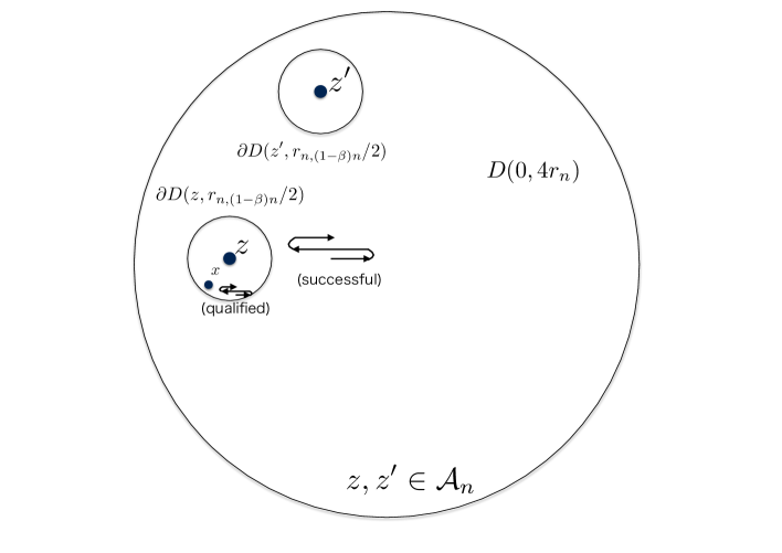
Figure 3.

Remark 6.9.

In [4], a slightly different scaling for the excursion counts was considered. Roughly speaking, they expected $\sqrt{\hat{N}_{n,l}^{z,x}}$ to be an almost linear function in $l$. However, as we later use the same method as in [1, 10, 20], we use almost the same definition of $r_{k}$.

Proposition 6.10.

As $n\to\infty$,

$$P\bigg{(} \bigg{\{}x\in D\bigg{(}z,\frac{r_{n,(1-\beta)n}}{2}\bigg{)}:x\text{ is }(n,\beta)\text{-qualified}\bigg{\}}$$

$$\subset \bigg{\{}x\in D\bigg{(}z,\frac{r_{n,(1-\beta)n}}{2}\bigg{)}:\frac{K(\hat{\mathcal{R}}^{z}_{(1-\beta)n,\tilde{f}((1-\beta)n)-(1-\beta)n},x)}{(\log K_{n})^{2}}\geq\frac{4\alpha}{\pi}-\frac{2}{\log\log n}\bigg{\}}\bigg{)}\to 1.$$

Proposition 6.11.

For $x\in D(z,r_{n,(1-\beta)n}/2)$,

$$P(x\text{ is }(n,\beta)\text{-qualified})=(1+o(1))q_{n},$$

where $q_{n}$ satisfies the following: there exist $c_{1}(\gamma,\alpha,\beta,\eta)$ and $c_{2}(\gamma,\alpha,\beta,\eta)>0$ such that, for all sufficiently large $n\in\mathbb{N}$,

$$e^{-c_{1}n\log\log n}K_{n}^{-2\alpha(1-\gamma(1-\beta))^{2}/\beta}\leq q_{n}\leq e^{-c_{2}n\log\log n}K_{n}^{-2\alpha(1-\gamma(1-\beta))^{2}/\beta}.$$

Proposition 6.12.

$(i)$ There exist $c_{3}(\gamma,\alpha,\beta)$ and $c_{4}(\gamma,\alpha,\beta)>0$ such that, for all sufficiently large $\eta\in\mathbb{N}$, $x,y\in D(z,r_{n,(1-\beta)n}/2)$ with $(1-\beta)n+\eta\leq l(x,y)\leq n$, and sufficiently large $n\in\mathbb{N}$,

$$P(x\text{ and }y\text{ are }(n,\beta)\text{-qualified})$$

$$\leq n^{c_{3}}e^{c_{4}(l-n+\beta n-\eta+1)\log\log n}q_{n}^{2}\exp\bigg{(}\frac{6\alpha}{\beta}(1-\gamma(1-\beta))^{2}(l-n+\beta n-\eta+1)\log n\bigg{)}.$$

$(ii)$ For all $x,y\in D(z,r_{n,(1-\beta)n}/2)$ with $l(x,y)\leq(1-\beta)n+\eta-1$,

$$P(x\text{ and }y\text{ are }(n,\beta)\text{-qualified})=(1+o(1))q_{n}^{2}.$$

Remark 6.13.

Note that the choice of sufficiently large $\eta\in\mathbb{N}$ is used instead of the sufficiently large $\overline{\gamma}>0$ in [1, 10].

Roughly speaking, Proposition 6.10 ensures that the set of qualified points is essentially a restriction of $\tilde{W}^{z}_{\tilde{f}((1-\beta)n)-(1-\beta)n}$. Propositions 6.11 and 6.12 are used to apply the second moment method based on the Paley–Zygmund inequality.

• We refer to the proof of [20, Lemma $3.1$] (see also [1, Proposition $3.3$]). Note that, for any $x\in D(z,r_{n,(1-\beta)n}/2)$,

  $$\bigg{\{}x\text{ is }(n,\beta)\text{-qualified}\bigg{\}}\cap\bigg{\{}\frac{K(\hat{\mathcal{R}}^{z}_{(1-\beta)n,\tilde{f}((1-\beta)n)-(1-\beta)n},x)}{(\log K_{n})^{2}}\geq\frac{4\alpha}{\pi}-\frac{2}{\log\log n}\bigg{\}}^{c}$$

  $$\subset \bigg{\{}K(\hat{\mathcal{R}}^{x}_{n,\hat{f}(n,n)-n},x)\leq\bigg{(}\frac{4\alpha}{\pi}-\frac{1}{\log\log n}\bigg{)}(\log K_{n})^{2}\bigg{\}}.$$

  As there exists some $c>0$ such that $|D(0,K_{n})|\leq e^{cn\log n}$ for all sufficiently large $n\in\mathbb{N}$, it is sufficient to prove that there exists some $c>0$ such that

  $$P\bigg{(}K(\hat{\mathcal{R}}^{x}_{n,\hat{f}(n,n)-n},x)\leq\bigg{(}\frac{4\alpha}{\pi}-\frac{1}{\log\log n}\bigg{)}(\log K_{n})^{2}\bigg{)}\leq\exp(-cn(\log n/\log_{2}n)^{2}).$$

  This proof is the same as that of [20, Lemma $3.1$]. Thus, it is omitted.

• Fix $x\in D(z,r_{n,(1-\beta)n}/2)$. Note that, from (3.7), we have that

  $$P^{x_{0}}(T_{\partial D(x,r_{n,l+1})}<T_{\partial D(x,r_{n,l-1})})=\frac{1}{2}(1+O(n^{-8}))$$

  for $(1-\beta)n+\eta\leq l\leq n-1$, $x_{0}\in\partial D(x,r_{n,l})$, as well as [20, $(4.14)$]. Then, for $x_{0}\in\partial D(x,r_{n,(1-\beta)n+\eta-1})$,

  $$P^{x_{0}}(T_{\partial D(z,r_{n,(1-\beta)n-1})}<T_{\partial D(x,r_{n,(1-\beta)n+\eta})})=(1+O(n^{-8}))\frac{1}{\eta+1}$$

  (see Figure 4).

  

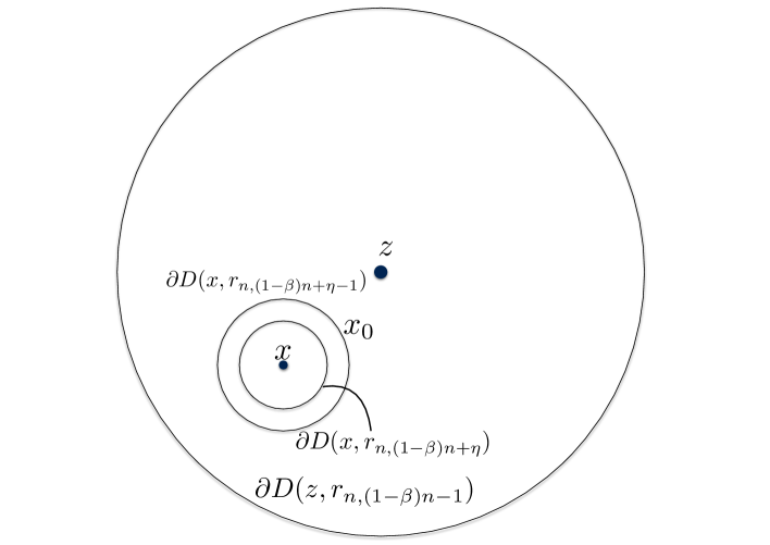
  Figure 4.

  In addition, for $m_{(1-\beta)n+\eta}$ with $|m_{(1-\beta)n+\eta}-\hat{f}(n,(1-\beta)n+\eta)|\leq n$, let

  $$\hat{q}_{n}:=\sum_{1\leq i\leq m_{(1-\beta)n+\eta}\wedge(\tilde{f}((1-\beta)n)-(1-\beta)n-1)} \bigg{(}\frac{\eta}{\eta+1}\bigg{)}^{\tilde{f}((1-\beta)n)-(1-\beta)n-1-i}\bigg{(}\frac{1}{\eta+1}\bigg{)}^{i}$$

  $$\begin{pmatrix}\tilde{f}((1-\beta)n)-(1-\beta)n-1\\ i\end{pmatrix} \bigg{(}\frac{1}{\eta+1}\bigg{)}^{i}\bigg{(}\frac{\eta}{\eta+1}\bigg{)}^{m_{(1-\beta)n+\eta}-i}\begin{pmatrix}m_{(1-\beta)n+\eta}-1\\ i\end{pmatrix}.$$

  Then, (3.5) and the same argument as for [1, Proposition $3.4$], [20, ($4.13$)], or [10, ($5.9$)] imply that

  (6.10) $$P(x\text{ is }(n,\beta)\text{-qualified})=P(|\hat{N}_{n,l}^{z,x}-\hat{f}(n,l)|\leq n\text{ for }(1-\beta)n+\eta\leq l\leq n)=(1+o(1))q_{n},$$

  where

  (6.13) $$q_{n}:=\sum\hat{q}_{n}\times\prod_{l=(1-\beta)n+\eta+1}^{n}\left(\begin{array}[]{cc}m_{l}+m_{l-1}-1\\ m_{l}\end{array}\right)\bigg{(}\frac{1}{2}\bigg{)}^{m_{l}+m_{l-1}-1}.$$

  Here, the summations in (6.10) and (6.13) cover all $m_{(1-\beta)n+\eta},\ldots,m_{n}$ with $|m_{l}-\hat{f}(n,l)|\leq n$ for $(1-\beta)n+\eta\leq l\leq n$. Hence, the Stirling formula implies that, for $m_{(1-\beta)n+\eta}$ with $|m_{(1-\beta)n+\eta}-\hat{f}(n,(1-\beta)n+\eta)|\leq n$,

  $$\hat{q}_{n}\geq \bigg{(}\frac{\eta}{\eta+1}\bigg{)}^{\tilde{f}(\beta n)-\beta n-1-i}\bigg{(}\frac{1}{\eta+1}\bigg{)}^{i}\begin{pmatrix}\tilde{f}(\beta n)-\beta n-1\\ i\end{pmatrix}\bigg{(}\frac{1}{\eta+1}\bigg{)}^{i}\bigg{(}\frac{\eta}{\eta+1}\bigg{)}^{m_{(1-\beta)n+\eta}-i}$$

  $$\begin{pmatrix}m_{(1-\beta)n+\eta}-1\\ i\end{pmatrix}\bigg{|}_{i=(2\eta\sqrt{\tilde{f}(\beta n)m_{(1-\beta)n+\eta}}-(m_{(1-\beta)n+\eta}+\tilde{f}(\beta n)-\beta n))/2(\eta^{2}-1)}$$

  (6.14) $$= n^{o(1)}.$$

  By the same estimate as in the proof of [1, Proposition $3.4$], we have that, for all $m_{i}$ with $|m_{i}-\hat{f}(n,i)|\leq n$ and $(1-\beta)n+\eta+1\leq l\leq n$,

  (6.17) $$\left(\begin{array}[]{cc}m_{l}+m_{l-1}-1\\ m_{l}\end{array}\right)\bigg{(}\frac{1}{2}\bigg{)}^{m_{l}+m_{l-1}-1}$$

  $$\geq c(m_{l})^{-1/2}\exp\bigg{\{}-m_{l-1}\bigg{(}\frac{1}{4}\bigg{(}\frac{m_{l}}{m_{l-1}}-1\bigg{)}^{2}+c^{\prime}\bigg{|}\frac{m_{l}}{m_{l-1}}-1\bigg{|}^{3}\bigg{)}\bigg{\}}$$

  $$\geq c(\log n)^{-cn}\exp\bigg{\{}-\frac{(m_{l}-m_{l-1})^{2}}{4m_{l-1}}\bigg{\}}$$

  $$\geq c(\log n)^{-cn}\exp\bigg{\{}-\frac{(6\alpha g_{l}^{2}\log n-6\alpha(g_{l}-(1/\beta-\gamma(1-\beta)/\beta))^{2}\log n)^{2}}{4m_{l-1}}\bigg{\}}$$

  $$\geq c(\log n)^{-cn}\exp\bigg{\{}-\frac{(12\alpha g_{l}(1/\beta-\gamma(1-\beta)/\beta)\log n)^{2}}{4m_{l-1}}\bigg{\}}$$

  $$\geq c(\log n)^{-cn}\exp\bigg{\{}-\frac{6\alpha g_{l}(1/\beta-\gamma(1-\beta)/\beta)^{2}\log n}{g_{l-1}}\bigg{\}}$$

  (6.18) $$\geq c(\log n)^{-cn}\exp\bigg{\{}-\frac{6\alpha}{\beta^{2}}(1-\gamma(1-\beta))^{2}\log n\bigg{\}},$$

  where $g_{l}:=l-(1-\beta)n/\beta+(n-l-(1-\beta)n/\beta)\gamma(1-\beta)$. Therefore, we obtain

  $$q_{n}\geq c(\log n)^{-cn}K_{n}^{-2\alpha(1-\gamma(1-\beta))^{2}/\beta},$$

  and hence, we have the desired lower bound. Note that (3.3) makes it trivial that $\hat{q}_{n}\leq 1$, and hence,

  $$\sum_{|m_{(1-\beta)n+\eta}-\hat{f}(n,(1-\beta)n+\eta)|\leq n}\hat{q}_{n}\leq n.$$

  If we use this instead of (6.14) and a computation such as (6.18), we have the upper bound.

To prove Proposition 6.12, we set the following sigma field, as in [1, 10]. First, we define a sequence of stopping times. Fix $z\in\mathcal{A}_{n}$ and $x\in D(z,r_{n,(1-\beta)n}/2)$. For $(1-\beta)n+\eta\leq l\leq n$, let $\sigma^{(0)}_{x}[l]:=0$ and

$$\tau_{x}^{(0)}[l] :=\inf\{m\geq 0:S_{m}\in\partial D(x,r_{n,l})\},$$

$$\sigma_{x}^{(i)}[l] :=\inf\{m\geq\tau_{x}^{(i-1)}[l]:S_{m}\in\partial D(x,r_{n,l-1})\}\text{ for }i\geq 1,$$

$$\tau_{x}^{(i)}[l] :=\inf\{m\geq\sigma_{x}^{(i)}[l]:S_{m}\in\partial D(x,r_{n,l})\}\text{ for }i\geq 1.$$

In addition, let $\mathcal{G}_{l}^{x}:=\sigma(\bigcup_{i\geq 0}\{S_{m}:\sigma^{(i)}_{x}[l]\leq m\leq\tau^{(i)}_{x}[l]\})$. Then, we obtain the following lemma.

Lemma 6.14.

There exists some $\epsilon_{n}$ with $\lim_{n\to\infty}\epsilon_{n}=0$ such that, for all $n-\beta n+\eta\leq l\leq n-1$ with $|m_{l}-\hat{f}(n,l)|\leq n$ and $x\in D(z,r_{n,(1-\beta)n}/2)$,

$$P(\hat{N}_{n,i}^{z,x}=m_{i}\text{ for all }i=l,\ldots,n|\mathcal{G}_{l}^{x})$$

$$= (1+\epsilon_{n})P(\hat{N}_{n,i}^{z,x}=m_{i}\text{ for all }i=l+1,\ldots,n|\hat{N}_{n,l}^{z,x}=m_{l})1_{\{\hat{N}_{n,l}^{z,x}=m_{l}\}}.$$

• The proof is the same as that of [10, Corollary $5.1$], because [10, Lemma $2.4$] holds even for a simple random walk in $\mathbb{Z}^{2}$ instead of one in a $2$-dimensional torus (see also [1, Lemma $3.6$]).

• The proof is almost the same as that of [1, Proposition $3.5$], as the argument in [1] holds even for a discrete-time simple random walk in $\mathbb{Z}^{2}$ instead of the continuous-time one with Lemma 6.14 (see also [20, Lemma $3.2$] or [10, Lemma $4.2$]). We now give an overview of the proof. As Proposition 6.12(i) yields Proposition 6.12(ii), we only prove the former. For $x,y\in D(z,r_{n,(1-\beta)n}/2)$ with $(1-\beta)n+\eta\leq l(x,y)\leq n$ and all sufficiently large $n\in\mathbb{N}$, Lemma 6.14 gives

  $$P(x\text{ and }y\text{ are }(n,\beta)\text{-qualified})$$

  $$\leq P(|\hat{N}_{n,i}^{z,x}-\hat{f}(n,i)|\leq n\text{ for all }i=(1-\beta)n+\eta,\ldots,l-3,l,\ldots,n$$

  $$\text{ and }|\hat{N}_{n,i}^{z,y}-\hat{f}(n,i)|\leq n\text{ for all }i=l,\ldots,n)$$

  $$\leq (1+o(1))\sum_{m_{l}:|m_{l}-\hat{f}(n,l)|\leq n}P(|\hat{N}_{n,i}^{z,x}-\hat{f}(n,i)|\leq n\text{ for all }i=(1-\beta)n+\eta,\ldots,l-3,l,\ldots,n$$

  $$\text{ and }|\hat{N}_{n,i}^{z,y}-\hat{f}(n,i)|\leq n\text{ for all }i=l+1,\ldots,n|\hat{N}_{n,l}^{z,y}=m_{l}).$$

  Then, it suffices to show the following:

  $$\sum_{m_{l}:|m_{l}-\hat{f}(n,l)|\leq n}P(|\hat{N}_{n,i}^{z,y}-\hat{f}(n,i)|\leq n\text{ for all }i=l+1,\ldots,n|\hat{N}_{n,l}^{z,y}=m_{l})$$

  (6.19) $$\leq n^{c}e^{c(l-n+\beta n+1)\log\log n}q_{n}\exp\bigg{(}\frac{6\alpha}{\beta}(1-\gamma(1-\beta))^{2}(l-n+\beta n-\eta+1)\log n\bigg{)},$$

  $$P(|\hat{N}_{n,i}^{z,x}-\hat{f}(n,i)|\leq n\text{ for all }i=(1-\beta)n+\eta,\ldots,l-3,l,\ldots,n)$$

  (6.20) $$\leq n^{c}e^{c(l-n+\beta n-\eta+1)\log\log n}q_{n}.$$

  First, we prove (6.19). By Proposition 6.11 and Lemma 6.14,

  $$(1+o(1))q_{n}$$

  $$= P(y\text{ is }(n,\beta)\text{-qualified})$$

  $$\geq (1+o(1))\sum_{m_{l}:|m_{l}-\hat{f}(n,l)|\leq n}P(|\hat{N}_{n,i}^{z,y}-\hat{f}(n,i)|\leq n\text{ for all }i=(1-\beta)n+\eta,\ldots,l-1;\hat{N}_{n,l}^{z,y}=m_{l})$$

  $$\times P(|\hat{N}_{n,i}^{z,y}-\hat{f}(n,i)|\leq n\text{ for all }i=l+1,\ldots,n|\hat{N}_{n,l}^{z,y}=m_{l}).$$

  By the same argument as in the proof of Proposition 6.11,

  $$P(|\hat{N}_{n,i}^{z,y}-\hat{f}(n,i)|\leq n\text{ for all }i=(1-\beta)n+\eta,\ldots,l-1;\hat{N}_{n,l}^{z,y}=m_{l})$$

  $$\geq n^{-c}e^{c(l-n+\beta n+1)\log\log n}q_{n}\exp\bigg{(}\frac{6\alpha}{\beta}(1-\gamma(1-\beta))^{2}(l-n+\beta n-\eta+1)\log n\bigg{)},$$

  and hence, we obtain (6.19). Next, we show (6.20). By Lemma 6.14, (6.19), and the same argument as the proof of Proposition 6.11, we have that, for all sufficiently large $\eta>0$,

  $$P(|\hat{N}_{n,i}^{z,x}-\hat{f}(n,i)|\leq n\text{ for all }i=(1-\beta)n+\eta,\ldots,l-3,l,\ldots,n)$$

  $$\leq (1+o(1))P(|\hat{N}_{n,i}^{z,x}-\hat{f}(n,i)|\leq n\text{ for all }i=(1-\beta)n+\eta,\ldots,l-3)$$

  $$\times \sum_{m_{l}:|m_{l}-\hat{f}(n,l)|\leq n}P(|\hat{N}_{n,i}^{z,x}-\hat{f}(n,i)|\leq n\text{ for all }i=l+1,\ldots,n|\hat{N}_{n,l}^{z,x}=m_{l})$$

  $$\leq n^{c}e^{c(l-n+\beta n-\eta+1)\log\log n}\exp\bigg{(}-\frac{6\alpha}{\beta}(1-\gamma(1-\beta))^{2}(l-n+\beta n-\eta+1)\log n\bigg{)}$$

  $$\times n^{c}e^{c(l-n+\beta n-\eta+1)\log\log n}q_{n}\exp\bigg{(}\frac{6\alpha}{\beta}(1-\gamma(1-\beta))^{2}(l-n+\beta n)\log n\bigg{)}$$

  $$\leq n^{c}e^{c(l-n+\beta n-\eta+1)\log\log n}q_{n}.$$

  Therefore, we obtain the desired result.

• As mentioned in Remark 6.13, we consider the same argument as in the proof of the lower bound in [1, Theorem $1.2$(i)] (or [10]). If we select $\eta$ such that $c_{3}<6\eta-7$ in Proposition 6.12, Propositions 6.11 and 6.12 state that, for all sufficiently large $n\in\mathbb{N}$,

  $$E\bigg{[}\bigg{|}\bigg{\{}x\in D\bigg{(}z,\frac{r_{n,(1-\beta)n}}{2}\bigg{)}:x\text{ is }(n,\beta)\text{-qualified}\bigg{\}}\bigg{|}\bigg{]}\geq(1+o(1))\bigg{|}D\bigg{(}z,\frac{r_{n,(1-\beta)n}}{2}\bigg{)}\bigg{|}q_{n},$$

  $$E\bigg{[}\bigg{|}\bigg{\{}(x,y)\in D\bigg{(}z,\frac{r_{n,(1-\beta)n}}{2}\bigg{)}^{2}:x,y\text{ are }(n,\beta)\text{-qualified, }l(x,y)\geq(1-\beta)n+\eta\bigg{\}}\bigg{|}\bigg{]}$$

  $$\leq \bigg{|}D\bigg{(}z,\frac{r_{n,(1-\beta)n}}{2}\bigg{)}\bigg{|}^{2}(1+o(1))n^{c_{3}}q_{n}^{2}\sum_{l=(1-\beta)n+\eta}^{n}n^{-6\eta+7-6(l-n+\beta n-\eta+1)}e^{c_{4}(l-n+\beta n-\eta+1)\log\log n}$$

  $$\leq o(1)E\bigg{[}\bigg{|}\bigg{\{}x\in D\bigg{(}z,\frac{r_{n,(1-\beta)n}}{2}\bigg{)}:x\text{ is }(n,\beta)\text{-qualified}\bigg{\}}\bigg{|}\bigg{]}^{2},$$

  and

  $$E\bigg{[}\bigg{|}\bigg{\{}(x,y)\in D\bigg{(}z,\frac{r_{n,(1-\beta)n}}{2}\bigg{)}^{2}:x,y\text{ are }(n,\beta)\text{-qualified, }l(x,y)\leq(1-\beta)n+\eta-1\bigg{\}}\bigg{|}\bigg{]}$$

  $$\leq (1+o(1))\bigg{|}D\bigg{(}z,\frac{r_{n,(1-\beta)n}}{2}\bigg{)}\bigg{|}^{2}q_{n}^{2}.$$

  Then,

  $$E\bigg{[}\bigg{|}\bigg{\{}x\in D\bigg{(}z,\frac{r_{n,(1-\beta)n}}{2}\bigg{)}:x\text{ is }(n,\beta)\text{-qualified}\bigg{\}}\bigg{|}^{2}\bigg{]}$$

  $$\leq (1+o(1))E\bigg{[}\bigg{|}\bigg{\{}x\in D\bigg{(}z,\frac{r_{n,(1-\beta)n}}{2}\bigg{)}:x\text{ is }(n,\beta)\text{-qualified}\bigg{\}}\bigg{|}\bigg{]}^{2}$$

  uniformly in $z\in\mathcal{A}_{n}$. In addition, Proposition 6.11 implies that, for all sufficiently large $n\in\mathbb{N}$,

  $$E\bigg{[}\bigg{|}\bigg{\{}x\in D\bigg{(}z,\frac{r_{n,(1-\beta)n}}{2}\bigg{)}:x\text{ is }(n,\beta)\text{-qualified}\bigg{\}}\bigg{|}\bigg{]}\geq K_{n}^{2\beta-2\alpha(1-\gamma(1-\beta))^{2}/\beta-\delta}.$$

  Then, by the Paley–Zygmund inequality, we have that, as $n\to\infty$,

  $$P\bigg{(}\bigg{|}\bigg{\{}x\in D\bigg{(}z,\frac{r_{n,(1-\beta)n}}{2}\bigg{)}:x\text{ is }(n,\beta)\text{-qualified}\bigg{\}}\bigg{|}\geq K_{n}^{2\beta-2\alpha(1-\gamma(1-\beta))^{2}/\beta-2\delta}\bigg{)}\to 1.$$

  Therefore, by Proposition 6.10, as $n\to\infty$,

  $$P\bigg{(} \bigg{|}\bigg{\{}x\in D\bigg{(}z,\frac{r_{n,(1-\beta)n}}{2}\bigg{)}:K(\hat{\mathcal{R}}^{z}_{(1-\beta)n,\tilde{f}((1-\beta)n)-(1-\beta)n},x)\geq\bigg{(}\frac{4\alpha}{\pi}-\frac{1}{\log\log n}\bigg{)}(\log K_{n})^{2}\bigg{\}}\bigg{|}$$

  $$\geq K_{n}^{2\beta-2\alpha(1-\gamma(1-\beta))^{2}/\beta-2\delta}\bigg{)}\to 1,$$

  and hence, the desired result holds for all sufficiently large $n\in\mathbb{N}$ with $1/\log_{2}n<\delta$.

Finally, to complete the proof of Lemma 6.8, we present the following lemma. We say that a point $z\in\mathcal{A}_{n}$ is $(n,\beta)$-pre-successful if $|\hat{N}_{n,k}^{z}-\tilde{f}(k)|\leq k$ for all $3\leq k\leq n-\beta n$.

Lemma 6.15.

There exists $\delta_{n}>0$ with $\lim_{n\to\infty}\delta_{n}=0$ such that

(6.21) $$\overline{q}_{n}:=\inf_{x\in\mathcal{A}_{n}}P(x\text{ is }(n,\beta)\text{-pre-successful})\geq r_{(1-\beta)n}^{-(2\gamma^{2}\alpha+\delta_{n})}.$$

Then, there exists some $c>0$ such that, for all $x\neq y\in\mathcal{A}_{n}$,

(6.22) $$P(x\text{ and }y\text{ are }(n,\beta)\text{-pre-successful})\leq c\overline{q}_{n}^{2}r_{l(x,y)}^{2\gamma^{2}\alpha+\delta_{l(x,y)}}.$$

• As mentioned in [7], (6.21) and (6.22) are essentially established in [20, Lemma $3.2$], although [20] considered the case in which $\beta=0$ and used a different $r_{n,k}$ from ours. We provide an overview of the proof. First, we show (6.21). Note that, from (3.7), for any $1\leq k\leq n-\beta n-1$ and $x\in\partial D(z,r_{n,k})$,

  $$P^{x}(T_{\partial D(z,r_{n,k+1})}<T_{\partial D(z,r_{n,k-1})})=\frac{1}{2}+O(n^{-8}).$$

  Using [20, Lemma $4.1$] and the same argument as in the proof of Proposition 6.11,

  $$\inf_{x\in\mathcal{A}_{n}}P(x\text{ is }(n,\beta)\text{-pre-successful})$$

  $$\geq (1+o(1))\sum_{m_{k}:|m_{k}-\tilde{f}(k)|\leq k}\prod_{k=3}^{n-\beta n-1}\begin{pmatrix}m_{k+1}+m_{k}-1\\ m_{k+1}\end{pmatrix}\bigg{(}\frac{1}{2}\bigg{)}^{m_{k+1}+m_{k}}$$

  (6.23) $$\geq r_{(1-\beta)n}^{-(2\gamma^{2}\alpha+\delta_{n})},$$

  and hence, we obtain (6.21). Next, we prove (6.22). As a result of applying Lemma 6.14,

  $$P(x\text{ and }y\text{ are }(n,\beta)\text{-pre-successful})$$

  $$\leq \sum_{m_{l}:|m_{l}-\tilde{f}(l)|\leq l}P(|\hat{N}_{n,k}^{x}-\tilde{f}(k)|\leq k\text{ for all }k=3,\ldots,l-3,l,\ldots,n;\hat{N}_{n,l}^{y}=m_{l};$$

  $$|\hat{N}_{n,k}^{y}-\tilde{f}(k)|\leq k\text{ for all }k=l+1,\ldots,n-\beta n)$$

  $$\leq CP(|\hat{N}_{n,k}^{x}-\tilde{f}(k)|\leq k\text{ for all }k=3,\ldots,l-3,l,\ldots,n)$$

  $$\sum_{m_{l}:|m_{l}-\tilde{f}(l)|\leq l}P(|\hat{N}_{n,k}^{y}-\tilde{f}(k)|\leq k\text{ for all }k=l+1,\ldots,n-\beta n|\hat{N}_{n,l}^{y}=m_{l}).$$

  By the same argument as (6.23) (see also [20, (4.29)]),

  (6.24) $$\sum_{m_{l}:|m_{l}-\tilde{f}(l)|\leq l}P(|\hat{N}_{n,k}^{y}-\tilde{f}(k)|\leq k\text{ for all }k=l+1,\ldots,n-\beta n|\hat{N}_{n,l}^{y}=m_{l})\leq c\overline{q}_{n}r_{l(x,y)}^{2\gamma^{2}\alpha+\delta_{l(x,y)}}.$$

  In addition, by Lemma 6.14,

  $$P(|\hat{N}_{n,k}^{x}-\tilde{f}(k)|\leq k\text{ for all }k=3,\ldots,l-3,l,\ldots,n)$$

  $$\leq P(|\hat{N}_{n,k}^{x}-\tilde{f}(k)|\leq k\text{ for all }k=3,\ldots,l-3,l,\ldots,n)$$

  $$\times \sum_{m_{l}:|m_{l}-\tilde{f}(l)|\leq l}P(|\hat{N}_{n,k}^{x}-\tilde{f}(k)|\leq k\text{ for all }k=l+1,\ldots,n|\hat{N}_{n,l}^{x}=m_{l}).$$

  By the same argument as for (6.23) and (6.24),

  $$P(|\hat{N}_{n,k}^{x}-\tilde{f}(k)|\leq k\text{ for all }k=3,\ldots,l-3,l,\ldots,n)\leq c\overline{q}_{n}r_{l(x,y)}^{\delta_{l(x,y)}}.$$

  With (6.24), we have (6.22).

• As an $(n,\beta)$-successful point is also an $(n,\beta)$-pre-successful point, (6.22) leads to (6.9). To show (6.9), we refer to the proof of [7, Lemma $2.1$] or [10, Lemma $10.1$]. Substitute $n$, $1-\beta$, $l(x,y)$, and $2\gamma^{2}\alpha$ for $m$, $\beta$, $k(x,y)$, and $a$ in [7, Lemma $2.1$], respectively, and consider our event $H_{(1-\beta)n}^{x}$ and $\sup_{x\in\mathcal{A}_{n}}P(H^{x}_{(1-\beta)n,\tilde{f}((1-\beta)n)-(1-\beta)n})$ in (6.6) instead of $H_{\beta m}^{x}$ and $\xi_{m}$ in [7]. Then, using Lemma 6.7 instead of [7, $(2.13)$], we have that

  (6.25) $$P(x\text{ is }(n,\beta)\text{-successful})\geq(1+o(1))P(x\text{ is }(n,\beta)\text{-pre-successful}).$$

  uniformly in $x\in\mathcal{A}_{n}$. An overview of the proof is as follows. By the same argument as in the proof of Lemma 6.14,

  $$P(|\hat{N}_{n,k}^{x}-\tilde{f}(k)|\leq k\text{ for all }k=3,4,\ldots,n-\beta n)$$

  $$= \sum_{m_{l}:|m_{l}-\tilde{f}(l)|\leq l}P(|\hat{N}_{n,k}^{x}-\tilde{f}(k)|\leq k\text{ for all }k=3,4,\ldots,n-\beta n-1;$$

  $$\quad\quad\quad\quad\quad\hat{N}_{n,n-\beta n}^{x}=m_{l};H^{x}_{(1-\beta)n,\tilde{f}((1-\beta)n)-(1-\beta)n})$$

  $$= (1+o(1))(1-\sup_{x\in\mathcal{A}_{n}}P(H^{x}_{(1-\beta)n,\tilde{f}((1-\beta)n)-(1-\beta)n}))P(|\hat{N}_{n,k}^{x}-\tilde{f}(k)|\leq k\text{ for all }k=3,4,\ldots,n-\beta n)$$

  $$= (1+o(1))P(|\hat{N}_{n,k}^{x}-\tilde{f}(k)|\leq k\text{ for all }k=3,4,\ldots,n-\beta n).$$

  Then, from Lemma 6.7,

  $$P(x\text{ is }(n,\beta)\text{-successful})\geq(1+o(1))P(|\hat{N}_{n,k}^{x}-\tilde{f}(k)|\leq k\text{ for all }k=3,4,\ldots,n-\beta n),$$

  and hence, we obtain (6.25). Therefore, with the aid of (6.21) and (6.25), we have (6.8).

- [1] Abe, Y. (2015). Maximum and minimum of local times for two-dimensional random walk. Electron. Commun. Probab., , no. 22, 1–14.
- [2] Bolthausen, E., Deuschel, J. D. and Giacomin, G. (2001). Entropic repulsion and the maximum of the two-dimensional harmonic crystal. Ann. Probab., , 1670–1692.
- [3] Brummelhuis, M. and Hilhorst, H. (1991). Covering of a finite lattice by a random walk. Phys. A, , 387–408.
- [4] Belius, D. and Kistler, N. (2016). The subleading order of two dimensional cover times. Probab. Theory Relat. Fields, , no. 1-2, 1–92.
- [5] Daviaud, O. (2006). Extremes of the discrete two-dimensional Gaussian free field. Ann. Probab., , 962–986.
- [6] Dembo, A. (2003). Favorite points, cover times and fractals. In Lectures on Probability Theory and Statistics, volume of Lecture Notes in Math., pages 1–101. Springer, Berlin. Lectures from the 33rd Probability Summer School held in Saint-Flour, July, 6–23.
- [7] Dembo, A., Peres, Y. and Rosen, J. (2007). How large a disc is covered by a random walk in n steps? Ann. Probab., , 577–601.
- [8] Dembo, A., Peres, Y., Rosen, J. and Zeitouni, O. (2001). Thick points for planar Brownian motion and the Erdős–Taylor conjecture on random walk. Acta Math., , 239–270.
- [9] Dembo, A., Peres, Y., Rosen, J. and Zeitouni, O. (2004). Cover times for Brownian motion and random walks in two dimensions. Ann. Math., , 433–464.
- [10] Dembo, A., Peres, Y., Rosen, J. and Zeitouni, O. (2006). Late points for random walks in two dimensions. Ann. Probab., , 219–263.
- [11] Ding, J. (2014). Asymptotics of cover times via Gaussian free fields: Bounded-degree graphs and general trees. Ann. Probab., , 464–496.
- [12] Ding, J., Lee, J. R. and Peres, Y. (2012). Cover times, blanket times, and majorizing measures. Ann. of Math., , 1409–1471.
- [13] Eisenbaum, N., Kaspi, H., Marcus, M. B., Rosen, J. and Shi, Z. (2000). A Ray–Knight theorem for symmetric Markov processes. Ann. Probab., , 1781–1796.
- [14] Erdős, P. and Révész, P. (1984). On the favourite points of a random walk. Mathematical Structures–Computational Mathematics–Mathematical Modelling, , 152–157. Sofia.
- [15] Erdős, P. and Révész, P. (1987). Problems and results on random walks. In: Mathematical Statistics and Probability (P. Bauer et al., eds.), Proceedings of the 6th Pannonian Symposium, Volume , 59–65.
- [16] Erdős, P. and Taylor, S. J. (1960). Some problems concerning the structure of random walk paths. Acta Sci. Hung., , 137–162.
- [17] Lawler, G. F. (1991). Intersections of Random Walks. Birkhauser, Boston.
- [18] Lifshits, M. A. and Shi, Z. (2004). The escape rate of favorite sites of simple random walk and Brownian motion, Ann. Probab., , 129–152.
- [19] Okada, I. (2016). Frequently visited sites of the inner boundary of random walk range. Stochastic Process. Appl., , 1412–1432.
- [20] Rosen, J. (2005). A random walk proof of the Erdős–Taylor conjecture. Periodica Mathematica Hungarica, , 223–245.
- [21] Shi, Z. and Tóth, B. (2000). Favourite sites of simple random walk. Periodica Mathematica Hungarica, , 237–249.