The effect of anisotropic exchange interactions and short-range phenomena on superfluidity in a homogeneous dipolar Fermi gas

Abstract

We develop a simple numerical method that allows us to calculate the Bardeen-Cooper-Schriefer (BCS) superfluid transition temperature ($T_{c}$) precisely for any interaction potential. We apply it to a polarised, ultracold Fermi gas with long-range, anisotropic, dipolar interactions and include the effects of anisotropic exchange interactions. We pay particular attention to the short-range behaviour of dipolar gasses and re-examine current renormalisation methods. In particular, we find that dimerisation of both atoms and molecules significantly hampers the formation of a superfluid. The end result is that at high density/interaction strengths, we find $T_{c}$ is orders of magnitude lower than previous calculations.

A great deal of interest in dipolar Fermi gasses has been generated due to their long range interactions, which lead to many novel effects such as p-wave superfluidity (Baranov et al., 2002, 2004; Baranov, 2008; Bruun and Taylor, 2008), topological superfluidity in 2D systems (Cooper and Shlyapnikov, 2009; Levinsen et al., 2011), anisotropic and many body effects on the Fermi liquid properties (Baranov et al., 2012; Krieg et al., 2015), the tailoring of novel interaction potentials (Büchler et al., 2007; Micheli et al., 2007), and superfluidity in bilayers (Pikovski et al., 2010; Baranov et al., 2011).

This rich selection of interesting phenomena has lead to a large effort from many groups to trap and cool a dipolar gas to degeneracy. Many highly successful experiments have resulted from this effort, which have concentrated on both molecular (Ospelkaus et al., 2010a; Ni et al., 2010; Ospelkaus et al., 2010b; de Miranda et al., 2011; Wu et al., 2012; Neyenhuis et al., 2012; Park et al., 2015) and atomic, highly-magnetic dipolar gasses (Lu et al., 2012; Aikawa et al., 2014a; Frisch et al., 2014; Baumann et al., 2014; Aikawa et al., 2014b, c; Naylor et al., 2015; Burdick et al., 2015). These experiments investigated features such as the precise control of ultracold chemical reactions (Ospelkaus et al., 2010b; Ni et al., 2010; de Miranda et al., 2011), quantum chaos in dipolar collisions (Baumann et al., 2014; Frisch et al., 2014), anisotropic interaction effects in the Fermi surface (Aikawa et al., 2014c), and dipolar collisions (Aikawa et al., 2014b). As yet, however, a dipolar Fermi superfluid has not been observed.

Predictions for the superfluid transition temperature of a dipolar Fermi gas ($T_{c}$) have been calculated in a number of works under various conditions (Baranov et al., 2002; Bruun and Taylor, 2008; Cooper and Shlyapnikov, 2009; Zhao et al., 2010; Pikovski et al., 2010; Baranov et al., 2011; Sieberer and Baranov, 2011; Levinsen et al., 2011; Liu et al., 2015). These works consider a dipolar Fermi gas within an idealised condensed matter paradigm, which is usually applicable for thermodynamically stable systems. However, an ultra-cold dilute gas is not stable. We investigate the complications that this introduces and produce our own predictions for Tc that differ significantly from these previous works at high densities or interaction strengths. After deriving our results, we compare our methodology with previous works in Section V.

This paper will be set out as follows. In Section I we review some important theoretical and experimental background involving the stability of p-wave gasses, particularly the collapse into p-wave dimers. We will then investigate how adding long-range interactions affects these p-wave dimers and produces dipolar-interaction-dominated bound states. In Section II we see that these dipolar bound states can have a large effect on the stability of the gas and therefore also on $T_{c}$. A key result of this paper is that we will show that in attempting to renormalise out the short range behavior of a dipolar gas, previous works in this area have ended up calculating a transition to tightly bound molecules, rather than to a BCS superfluid. We will then suggest a remedy to this problem.

Section III describes a simple algorithm that allows one to easily calculate the BCS transition temperature for complicated potentials. Furthermore, it allows us to take into account the effect of an anisotropic Fermi surface (in this case caused by the anisotropic interaction potential of a polarised dipolar gas). This is a general algorithm that can be applied to any system. In Section IV we apply the numerical method from Section III to the theoretical method of Section II to obtain prediction for $T_{c}$ at different experimental parameters. We find that in the region of experimental interest (i.e., high interaction strength or high densities) is where our results differ from previous theoretical works in this area, giving us a $T_{c}$ which is much lower. In Section V we will then compare our results to this previous theoretical work in more detail with the aim of understanding how and why they differ.

I Understanding the role of dipolar bound states and the centrifugal barrier.

Dipolar gas experiments face a number of challenges, which include dipolar spin-flip collisions in atoms (Burdick et al., 2015), chemical reactions in dipolar molecules (Ni et al., 2010; Ospelkaus et al., 2010b; de Miranda et al., 2011), and long-lived scattering chain complexes (Mayle et al., 2013). Because s-wave interactions are not allowed between identical fermions, all these effects can be protected against using the centrifugal barrier in the p-wave (and higher) scattering channels to prevent two scattering dipoles from coming into contact. The great effectiveness of the p-wave barrier in protecting the gas from inelastic processes has been shown in a series of experiments involving $\mathrm{{}^{40}K^{87}Rb}$ molecules at JILA (Ni et al., 2010), which are prone to react chemically (via $\mathrm{KRb+}$$\mathrm{KRb}\rightarrow$$\mathrm{K}_{2}+$$\mathrm{Rb_{2}}$), as well as in Dy atoms, which undergo spin flip collisions (Burdick et al., 2015).

To help understand the properties of the centrifugal barrier in the presence of dipolar interactions, we recall the results of Ref. (Quéméner and Bohn, 2010). In that work, it was shown that the attribute of interest is the height, $V_{b}$, of the barrier with the lowest maximum strength (which is the $l=1$, $m=0$ barrier) and how this compares with the average particle kinetic energy. It was also shown that the location and height of this barrier varies as the interactions strength, $C_{dd}$, changes, with $V_{b}$ decreasing as $C_{dd}$ increases, and finally it was shown that for sufficiently strong $C_{dd}$, $V_{b}$ is completely determined by $C_{dd}$ and is independent of the short range specifics of the potential. The result is that within this regime (Quéméner and Bohn, 2010)

$$r_{b}=\alpha\frac{C_{dd}m}{\hbar^{2}},$$ (1)

where $\alpha=0.6$, and $m$ is the mass of the particles. We will use units such that $r_{b}=1$, $\hbar=1$, $k_{B}=1$, and $m=1$, giving units of energy $E_{D}=\hbar^{2}/mr_{b}^{2}=\hbar^{6}/m^{3}C_{dd}^{2}\alpha^{2}$. In these units, $C_{dd}=1/\alpha$ and $V_{b}=2/3$ are both constants. All our equations will reduce down to just two dimensionless parameters: the dimensionless temperature $\mathfrak{\tau}=T/E\propto T/C_{dd}^{2}$, and the dimensionless average distance between atoms $\lambda=\rho^{-1/3}/r_{b}\propto C_{dd}\,^{-1}$, where $\rho=k_{F}{}^{3}/6\pi^{2}$ is the density, and $k_{F}$ is the Fermi surface (which gives $\lambda\approx 3.9/r_{b}k_{F}$). Ref. (Quéméner and Bohn, 2010) shows, as is verified by experiments (Ni et al., 2010), that as the average particle kinetic energy approaches $V_{b}$, the rate of barrier transmission nears unity, and quenching rates become unacceptably high. We note, as a benchmark for this effect, that the Fermi energy intersects $V_{b}$ at $\lambda\approx 3.38$.

An important conclusion from Eq. (1) is that in a gas with polarised dipolar interactions, the centrifugal barrier is much farther away from $r=0$ than a gas with short range interactions. Because dipole interactions are strongly attractive in the $l=1$, $m=0$ subspace, they can lead to dipolar bonding between dipoles (Wang et al., 2011; Wang and Greene, 2012). These dipole-induced, p-wave dimers will be of the size of the centrifugal barrier and will therefore be much larger than the p-wave bound states found in typical gasses with short-range interactions. The formation of p-wave dimers is significant because they are well known to be unstable from investigations in systems of identical fermions with short-range interactions near a p-wave resonance. These systems were first shown to be experimentally unstable (Regal et al., 2003; Ticknor et al., 2004; Zhang et al., 2004; Schunck et al., 2005; Günter et al., 2005; Gaebler et al., 2007; Fuchs et al., 2008; Inada et al., 2008; Maier et al., 2010; Nakasuji et al., 2013), then it was then shown that the major cause of this instability could be attributed to the fact that p-wave dimers, which are formed rapidly via three-body interactions when near the resonance, are unstable to collisional relaxation and decay much faster than they can thermalise (Levinsen et al., 2007; D’Incao et al., 2008; Levinsen et al., 2008; Jona-Lasinio et al., 2008; Fuchs et al., 2008). It has been shown that this behavior is a general property of identical fermions, and not of any property of the particular species being investigated (Levinsen et al., 2007).

In Fig. 1, we investigate the behavior of a p-wave dimer of two particles with strong dipolar interaction. The exact details of the interaction potential is species dependent; however, for particles with strong dipolar interactions, which are of interest to us, the largest bound states are dominated by the bare dipolar interaction. We have solved the Schrödinger equation using the finite element method (Ram-Mohan, 2002) for a bare dipolar interaction with a cutoff, $R_{cut}$, and plotted the energy and the root-mean-squared widths of the eigenstates. The short-range behavior is unknown, so we have plotted these eigenstates for a continuously varying value of $R_{cut}$ (filled and dashed lines), showing the effect that different short-range behaviour can have on the bound states of a dipolar-long-range-dominated interaction potential. The figure shows the typical behavior of the bound states, which are evenly spaced and increase in size as $R_{cut}$ increases. Just before the energy of a bound state crosses zero, the bound state is at its largest, with a root-mean-square extent of $2.1r_{b}$. Just after the energy goes above zero, the bound state disappears and the next bound state becomes the largest, which is always sitting at around $0.15r_{b}$. We can therefore conclude that no matter the short-range specifics, the root mean squared size of the largest bound state will be within the range $0.15r_{b}$ and $2.1r_{b}$.

Three-body dimerisation rates for identical dipolar fermions have been explicitly calculated in (Wang et al., 2011), but not relaxation rates. In the s-wave case, the increasing size of a dimer leads to stability against inelastic relaxation collisions as the distance between the shallowest dimer and the deeply-bound states increases (Levinsen et al., 2007; Petrov, 2003; Petrov et al., 2004, 2005; Esry et al., 2001; Suno et al., 2003). In the dipolar case, the sizes of the deeply bound states increase along with the size of the shallowest dimer, negating that protection. Fig. 1 shows that once a weakly bound dimer of two dipoles is formed, there is cascade of nearby tighter bound states that the dimer can easily decay into. These dimers can then be expected to be unstable just as for the short-range case.

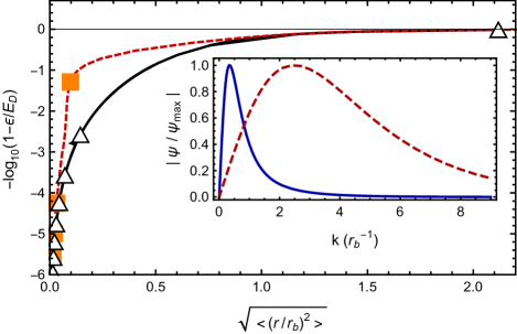
Figure 1: The bound state energies vs the root mean square size of the corresponding wavefunctions for a dipolar potential with a cutoff at $R_{cut}$. The triangles and squares represent bound states at $R_{cut}=0.01093r_{b}$, just before the largest bound state disappears. As $R_{cut}$ varies, all the squares move along the exact same dashed line, and all the triangles move along the same solid line. The triangle states are $l=1$ and 3 dominated. The square states are $l=5$ and 7 dominated. Interestingly, the bound states are all evenly spaced along each line. For example, depicted here the $7^{{\rm th}}$ triangle, sitting at $2.1r_{b}$, is about to disappear and the $6^{{\rm th}}$ triangle sits at $0.15r_{b}$. If we continue to increase $R_{cut}$ until the $6^{{\rm th}}$ triangle is about to disappear, we find that the $6^{{\rm th}}$ triangle will be at $2.1r_{b}$ and the $5^{{\rm th}}$ triangle at $0.15r_{b}$, almost exactly where the $6^{{\rm th}}$ triangle is now. Hence we can infer that the possible sizes of the largest bound state should sit within the range $0.15r_{b}$ to $2.1r_{b}$. Inset: the wavefunction in momentum space of the eigenstate that is on resonance (filled line), and the next shallowest bound state (dashed line). Both are the $l=1$, $m=0$ component. The filled line is therefore the largest possible dimer (occuring when the potential is on resonance). The dashed line is the smallest possible size for the shallowest dimer (occurs when the largest bound state disappears).

II The effect of dipolar bonding on $T_{c}$

Here we will show that the formation of these p-wave dimers is also extremely important for the renormalisation of the BCS equations. The BCS equations find the minimum of the free energy. It is well known from the BCS-BEC crossover problem (Nozières and Schmitt-Rink, 1985) that if the full potential is considered, the BCS equations will simply converge to the tightest bound state and form tightly bound bosons. Ultra-cold gasses are meta-stable, and we are not interested in the absolute ground state. For this reason, the BCS equations are usually renormalised using the method of Randiera et. al (Randeria et al., 1989, 1990). The purpose being to remove the short range behavior, but capture accurately the long range scattering properties of the atoms involved. A similar method must be implemented for the case we are interested in: a meta-stable gas of dipoles that sit outside each others centrifugal barriers and interact only via the universal, long-range dipolar interaction.

Predictions for $T_{c}$ of a dipolar Fermi gas under various conditions have been calculated in a number of works (Baranov et al., 2002; Bruun and Taylor, 2008; Cooper and Shlyapnikov, 2009; Zhao et al., 2010; Pikovski et al., 2010; Baranov et al., 2011; Sieberer and Baranov, 2011; Levinsen et al., 2011; Liu et al., 2015). The most common method used is to introduce the renormalised equations of Randiera et.al., except instead of replacing the T matrix with its long-range behavior via a first order expansion in $k$ (i.e., $4\pi\hbar^{2}a/m$), the Born approximation is used to replace the T-matrix by the bare potential. However, it is not clear that the short-range behavior is removed with this technique. Indeed, the bare dipolar potential contains all powers of $k$, meaning short-range behavior is merely modified, not removed. In fact, if we examine Fig. 2 in Ref. (Baranov et al., 2002) or Fig. 3(b) in Ref. (Liu et al., 2015), we can see that, for sufficiently large $k_{F}$, the gap plotted in those works is the same size and shape as the two-body bound state plotted in the inset in Fig. 1 in this work. For $k_{F}\approx 0.5/r_{b}$ ($\lambda=7.8$) the gap in those works is the same size and shape as the largest possible size for the shallowest dimer (filled line in inset in Fig. 1). For $k_{F}\approx 2.5/r_{b}$ ($\lambda=1.56$) the gap in those works is the same size and shape as the smallest possible size for the shallowest dimer (dashed line in inset in Fig. 1). A true BCS pairing wavefunction should be many times the size of the inter-particle spacing, not the size of a bound state. This suggests that the BCS equations, renormalised in this way, have simply picked up the tightly bound p-wave dimers that we expect to be unstable. In other words, at high densities/interaction strengths, these papers are calculating the transition to a tightly bound BEC state rather than the desired BCS state.

In this paper we produce our own predictions for a 3D, polarized, dipolar Fermi gas in a way that deals with these issues. We first consider just the case of the KRb experiment at JILA, the solution of which will turn out to be relevant to all systems discussed above. We require a methodology which can describe a situation where the gas is in quasi-stable equilibrium with molecules sitting outside each others centrifugal barriers, and as soon as the particles tunnel, they are almost guaranteed to be lost from the trap. We know that the solutions should be independent of the short range details of the molecules and should depend only on the $r^{-3}$ dipolar interaction. However, if we were to simply use the bare dipolar interaction, the BCS equations would only pick up the tightly-bound states that sit well within the centrifugal barrier and do not represent the meta-stable equilibrium that is desired.

The problem is that the dipolar interaction becomes very strong inside the centrifugal barrier, but in the KRb experiments at JILA, the molecules in quasi-stable equilibrium never “feel” that part of the potential, and any particles that do venture within each others centrifugal barrier undergo inelastic collisions with close to unit probability(Quéméner and Bohn, 2010; Ni et al., 2010) and consequently cannot contribute to the superfluid. We therefore use the following effective potential, which represents the anisotropic interaction between meta-stable dipoles that are polarized in the $\hat{\mathbf{z}}$ direction.

$$V_{\mathrm{dd}}^{\mathrm{(eff)}}(\mathbf{r})=\begin{cases}C_{dd}\frac{1}{r^{3}}\left(1-3\cos^{2}(\theta_{r})\right)&r>r_{b}\\ 0&r<r_{b}\end{cases},$$ (2)

where $C_{dd}$ is the interaction coupling constant. $\theta_{r}$ is the angle between $\mathbf{r}$ and the $\hat{\mathbf{z}}$ axis. Eq. (2) is just the usual dipolar potential (Ticknor, 2008), except cutoff at $r=r_{b}$. By using Eq. (2), we can minimise the free energy without picking up the undesired bound states, and the dipoles will feel the full dipolar potential outside the centrifugal barrier, but not inside, exactly as the molecules in the JILA experiments do. Furthermore, Eq. (2) reproduces the desired universal, dipolar-scattering amplitudes (Ticknor, 2008; Bohn et al., 2009), which means that provided the short range contribution to the potential does not put the system on resonance, Eq. (2) contains the key properties desired from a more conventional renormalisation method (see the discussion in Section V).

III Numerical method

We use the following method to find $T_{c}$, which is generally applicable to any potential, and can easily include the effects of the anisotropic exchange interactions. First recall the standard result that the BCS equations are equivalent to minimising the BCS free energy ($F$) (De Gennes, 1999). This free energy can be written in terms of the gap, $\Delta(\mathbf{k})$, the potential in momentum space, $V(\mathbf{k})$, and the non-superfluid part of the quasi-particle energy, $\kappa(\mathbf{k})=\hbar^{2}k^{2}/2m-\mu+\Sigma(\mathbf{k})$, where $\Sigma$ is the self energy and includes the Hartree and Fock energies:

$$F = E_{0}+E_{B}-TS,$$ (3a)

$$E_{0} = {\rm V}\int\frac{\mathrm{d^{3}}\mathbf{k}}{(2\pi)^{3}}\kappa(\mathbf{k})G_{\mathbf{k}},$$ (3b)

$$E_{B} = \frac{{\rm V}}{2}\int\frac{\mathrm{d^{3}}\mathbf{k}}{(2\pi)^{3}}\int\frac{\mathrm{d^{3}}\mathbf{k^{\prime}}}{(2\pi)^{3}}J_{\mathbf{k}}^{*}V(\mathbf{k},\mathbf{k^{\prime}})J_{\mathbf{k^{\prime}}},$$ (3c)

$$S = -{\rm V}\int\frac{\mathrm{d^{3}}\mathbf{k}}{(2\pi)^{3}}f_{\mathbf{k}}\log(f_{\mathbf{k}})+(1\!-\!f_{\mathbf{k}})\log(1\!-\!f_{\mathbf{k}}).\quad$$ (3d)

$$J_{\mathbf{k}} = \frac{-\Delta(\mathbf{k})}{2E(\mathbf{k})}\tanh(\frac{E(\mathbf{k})}{2T}),$$ (3e)

$$G_{\mathbf{k}} = \frac{\kappa(\mathbf{k})}{2E(\mathbf{k})}\tanh(\frac{E(\mathbf{k})}{2T})+\frac{1}{2}.$$ (3f)

$$\Sigma(\mathbf{k}) = \int\frac{\mathrm{d}^{3}\mathbf{q}}{(2\pi)^{3}}\left\{\bar{V}_{dd}(0)G(\mathbf{q})-V(\mathbf{k}-\mathbf{q})\mbox{G($\mathbf{q})$}\right\},$$ (3g)

$E(\mathbf{k})=\sqrt{\kappa(\mathbf{k})^{2}+\Delta(\mathbf{k})^{2}}$ is the full quasi-particle energy, $f_{\mathbf{k}}=(1+e^{E(\mathbf{k})/T})^{-1},$ V is the volume, $V(\mathbf{k})=\int e^{i\mathbf{k}\cdot\mathbf{r}}V_{\mathrm{dd}}^{\mathrm{(eff)}}(\mathbf{r})\mathrm{d}^{3}\mathbf{r}$, $V(\mathbf{k},\mathbf{k^{\prime}})=V(\mathbf{k}-\mathbf{k^{\prime}})$, $\kappa(\mathbf{k})=\xi(k)+\Sigma(\mathbf{k})$, $\xi(k)=\varepsilon_{0}(k)-\mu$, $\varepsilon_{0}(k)=\hbar^{2}k^{2}/2m$, $G_{\mathbf{k}}=\left\langle\hat{a}^{+}_{\mathbf{k}}\hat{a}_{\mathbf{k}}\right\rangle$, $J_{\mathbf{k}}=\left\langle\hat{a}_{\mathbf{-k}}\hat{a}_{\mathbf{k}}\right\rangle$, and $f_{\mathbf{k}}=\left\langle\hat{\gamma}^{+}_{\mathbf{k}}\hat{\gamma}_{\mathbf{k}}\right\rangle$, where $\hat{a}^{+}_{\mathbf{k}}$ and $\hat{a}_{\mathbf{k}}$ are the creation and annihilation operators of particle in momentum eigenstate $\mathbf{k}$, and $\hat{\gamma}$ is the quasiparticle operator satisfying $\left\langle\hat{\gamma}^{+}_{\mathbf{k}}\hat{\gamma}_{\mathbf{k}}\right\rangle=\delta_{\mathbf{k},\mathbf{k}}$, $\left\langle\hat{\gamma}_{\mathbf{k}}\hat{\gamma}_{\mathbf{k}}\right\rangle=0$, and $\hat{\gamma}_{\mathbf{k}}=u_{\mathbf{k}}\hat{a}^{+}_{\mathbf{k}}+v_{\mathbf{k}}\hat{a}_{\mathbf{k}}$ for c-numbers $u_{\mathbf{k}}$ and $v_{\mathbf{k}}$.

Note that the BCS transition is a second order phase transition with order parameter $\Delta$; therefore, it occurs at the point where $\Delta=0$ goes from being a minimum of the free energy with respect to $\Delta$ to a maximum or saddle point. Hence, only the Hessian of $F$ with respect to $\Delta$ needs to be calculated. The transition temperature is then simply the point where a negative eigenvalue occurs.

We will also need $V(\mathbf{k})$ in spherical components:

$$V(\mathbf{k},\mathbf{k^{\prime})}=\sum_{ll^{\prime}m}Y_{l}^{m}(\hat{\mathbf{k}})V_{ll^{\prime}}^{m}(k,k^{\prime})Y_{l^{\prime}}^{*m}(\hat{\mathbf{k^{\prime}}}),$$ (4)

$$V_{ll^{\prime}}^{m}(k,k^{\prime})=-\frac{(4\pi)^{2}}{\alpha}\sqrt{\frac{16\pi}{5}}i^{l^{\prime}-l}(-1)^{m}I_{ll^{\prime}}^{m}J_{ll^{\prime}}(k,k^{\prime}),\!$$ (5)

$$J_{ll^{\prime}}(k,k^{\prime})=\int_{1}^{\infty}\!\frac{\mathrm{d}r}{r}j_{l}(kr)j_{l^{\prime}}(k^{\prime}r),$$ (6)

$$I_{ll^{\prime}}^{m}=\sqrt{\frac{(2l+1)5(2l^{\prime}+1)}{4\pi}}\begin{pmatrix}l&2&l^{\prime}\\ 0&0&0\end{pmatrix}\begin{pmatrix}m&0&-m\\ l&2&l^{\prime}\end{pmatrix}.$$ (7)

Because we are dealing with identical p-wave fermions, we need only consider odd angular momenta, $l$. Also, $V_{ll^{\prime}}^{m}$ is non-zero only when $l^{\prime}=l$, or $l^{\prime}=l\pm 2$ (Bohn et al., 2009). Notice that the dipolar interactions conserve the angular momentum projection $m$. We will also need the self energy, which in a polarised dipolar gas is anisotropic and, because the Hartree term is zero, comes from the exchange interactions only; i.e., $-(2\pi)^{-3}\int\mathrm{d}^{3}\mathbf{q}V(\mathbf{k}-\mathbf{q})\mbox{G($\mathbf{q})$}$. We take $G\approx G_{0}=\theta(k_{F}-k)$, where $\theta$ is the Heaviside theta function, which gives

$$\Sigma(\mathbf{k}) =\frac{-1}{2\pi}\left(1-3\cos^{2}(\theta_{k})\right)\sigma(k),$$ (8)

$$\sigma(k) =\int_{1}^{\infty}\frac{1}{r^{4}}\left(\sin(k_{F}r)-k_{F}r\cos(k_{F}r)\right)j_{2}(kr)\mathrm{d}r.$$ (9)

Notice that $\Sigma$ also conserves the angular momentum projection. In order to solve the problem numerically, we must discretize the radial $k$ direction and choose a maximum angular momentum ($l_{max}$). We define a set of $n+1$ vertices, $x_{i}$, with $i\in[0,n]$, $x_{0}=0$, and $x_{i}>x_{i-1}$, then we consider only the set of $\Delta(\mathbf{k})$ functions that are constant when $k$ lies between vertices. We also discretize $V(\mathbf{k})$ on this grid. That is, we let

$$\Delta(\mathbf{k}) \rightarrow\sum_{l=\mathrm{odd}}^{l_{max}}\sum_{m=0}^{l}\sum_{i=1}^{n}\tilde{\Delta}_{l}^{m}(i)\mathcal{U}_{x_{i-1}}^{x_{i}}(k)Y_{l}^{m}(\hat{\mathbf{k}}),$$ (10a)

$$\bar{V}_{ll^{\prime}}^{m}\left(i,j\right) \equiv V_{ll^{\prime}}^{m}\Bigl{(}\frac{x_{i-1}+x_{i}}{2},\frac{x_{j-1}+x_{j}}{2}\Bigr{)},$$ (10b)

$$V_{ll^{\prime}}^{m}(k,k^{\prime}) \rightarrow\sum_{i,j=1}^{n}\mathcal{U}_{x_{i-1}}^{x_{i}}(k)\bar{V}_{ll^{\prime}}^{m}\left(i,j\right)\mathcal{U}_{x_{j-1}}^{x_{j}}(k^{\prime}),$$ (10c)

$$\mathcal{U}_{x_{i-1}}^{x_{i}}(k) \equiv\begin{cases}1&k\in[x_{i-1},x_{i}]\\ 0&\mathrm{otherwise}\end{cases}.$$ (10d)

We now use these discrete forms and Eq. (9) to calculate the free energy, $F$. Then, we take the double derivative of $F$ with respect to $\tilde{\Delta}$. Much cancellation occurs giving the following surprisingly simple result for the discretized Hessian matrix ($\mathcal{H}$) of $F$ with respect to the spherical components of the gap.

$$\mathcal{\bar{H}}_{lmi}^{l^{\prime}m^{\prime}j}=\left.\frac{\partial^{2}F}{\partial\tilde{\Delta}_{l}^{m*}(i)\partial\tilde{\Delta}_{l^{\prime}}^{m^{\prime}}(j)}\right|_{\Delta=0}=\frac{\mathrm{V}\delta_{mm^{\prime}}}{2(2\pi)^{3}}\mbox{$\times$}\\ \biggl{\{}\!K_{ll^{\prime}}^{m}(i)\delta_{ij}+\!\frac{1}{(2\pi)^{3}}\sum_{\bar{l}\,\bar{\bar{l}}}K_{l\bar{l}}^{m}(i)V_{\bar{l}\,\bar{\bar{l}}}^{m}(i,j)K_{\bar{\bar{l}}l^{\prime}}^{m}(j)\!\biggr{\}},$$ (11)

where the K matrix is given by

$$K_{l,l^{\prime}}^{m}(i) \equiv \int\mathrm{d}\hat{\mathbf{k}}K(i,\hat{\mathbf{k}})Y_{l}^{m*}(\hat{\mathbf{k}})Y_{l^{\prime}}^{m}(\hat{\mathbf{k}}),$$ (12)

$$K(i,\hat{\mathbf{k}}) = \int_{x_{i-1}}^{x_{i}}\mathrm{d}k\frac{k^{2}\tanh\left(\frac{\kappa(\mathbf{k})}{2T}\right)}{2\kappa(\mathbf{k})}.$$ (13)

Calculating whether the gas will be superfluid at a certain temperature and density requires only the calculation of the $K$ and $V$ matrices and then finding the lowest eigenvalue of the term inside the brackets in Eq. (11).

This method is applicable to any Hamiltonian for a homogeneous gas. The only difficult numerics arise from calculating the the $K$ matrix and a $\int_{1}^{\infty}\!\frac{\mathrm{d}r}{r}j_{l}(kr)j_{l^{\prime}}(k^{\prime}r)$ integral that appears in $V_{l\,l^{\prime}}^{m}$. The integral (with perhaps a different power of $r$) is common to any potential, as is the whole $K$ matrix, and it turns out that analytic solutions exist for both these functions that are valid for most points on the grid. This means the Hessian can be calculated easily and efficiently. Details are given in the Appendix.

IV Numerical Results

Results using this methodology for $T_{c}$, including the effect of anisotropic exchange interactions, are shown in Fig. 2. We use $l=1$ and $l=3$ contributions, $l=5$ makes almost no difference to $T_{c}$. Also shown is the previous calculation from Ref. (Baranov et al., 2002). Our inclusion of $l=3$ states as well as exchange interactions gives us a slightly higher $T_{c}$ at low densities. At higher densities, the drop in $T_{c}$ reflects the fact that Ref. (Baranov et al., 2002) is picking up contributions from p-wave dimers as discussed above. The inset shows the effect of just considering $l=1$ and the effect of turning off exchange interactions, which demonstrates that exchange interactions can either increase or decrease $T_{c}$ depending on the circumstances.

But what about the case of dipolar molecules that are chemically stable against two-body collision(Żuchowski and Hutson, 2010), such as $\mathrm{{}^{23}Na^{40}K}$ (Wu et al., 2012; Park et al., 2015), or dipolar atoms? In a typical gas with short-range interactions, three-body losses are proportional to the probability that two particles will approach within a distance equal to the size of their bound state, and that a third particle will venture within interactions range to take away excess kinetic energy. For dipoles, we can see that for inelastic scattering to occur, two dipoles must approach within each others centrifugal barrier, but, due to long range interactions, the third can absorb excess energy from a distance. Worse still, because the gas interaction energy is not extensive, the whole gas can effectively absorb excess energy from a collision pair simultaneously.

Referring back to Fig. 2, and comparing the filled and dashed lines, we see that the cutoff only starts to affect $T_{c}$ around $\lambda\lesssim 5$. At these densities, the average distance between dipoles is only 2 to 30 times larger than the size of the shallowest dimers (see the discussion in Fig. 1). This is much smaller than is normal for typical dilute gasses with short-range interactions. Given that once the molecules have tunneled they can dimerise by expelling energy to multiple external dipoles at once, and given their proximity to these other dipoles, it is not unreasonable to expect dimerisation to occur at very high probability inside the centrifugal barrier (This also agrees with exact numerical calculations that give a three-body recombination rate of dipolar fermions proportional to $C_{dd}^{8}$ (Wang et al., 2011)). If we combine this with the possibility of long lived scattering chain complexes (Mayle et al., 2013), and of inelastic spin-flip interactions in atoms(Lu et al., 2012), then to us it seems reasonable that our effective potential should be valid also for chemically stable molecules and dipolar atoms as well (for dipolar atoms, the bound states in Fig. 1 just represent the shallowest rovibrational states of a molecule).

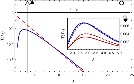
Figure 2: Predictions for $T_{c}$ in a dipolar Fermi gas. $\lambda$ is the dimensionless average distance between dipoles given by $(6\pi^{2})^{1/3}/(k_{F}\alpha C_{dd}m\hbar^{-2})$. The straight line at the top is the position of the Fermi energy, $T=T_{F}$. The solid blue line is our full numeric calculation. The dashed red line is the theoretical prediction given in Ref. (Baranov et al., 2002). The markers are the locations of current experiments: $\mathrm{{}^{40}K^{87}Rb}$(Ni et al., 2010) at the theoretical maximum polarisation (△), $\mathrm{{}^{40}K^{87}Rb}$(Ni et al., 2010) at current experimental polarisations (○) $\mathrm{{}^{23}Na^{40}K}$(Park et al., 2015) at the theoretical maximum polarisation (▲), $\mathrm{{}^{161}Dy}$(Lu et al., 2012) (⬥),$\mathrm{{}^{167}Er}$ (Aikawa et al., 2014a) (⬦), and $\mathrm{{}^{53}Cr}$(Naylor et al., 2015) is not plotted as it sits too far off to the right. Inset: $T_{c}$ vs $\lambda$ zoomed in at the peak in $T_{c}$. The bottom two lines (Red) are with just $l=1$. The top two lines (blue) are with $l=1,3$. The dashed lines are the results with exchange interactions switched off. The upper solid (blue) line in the inset corresponds to the solid (blue) line in the outer plot.

V Discussion

Comparison with other work

It is worthwhile to now compare our results to those of Ref. (Baranov et al., 2002) to understand where and how they differ. In Ref. (Baranov et al., 2002), the same calculation was performed, except using the renormalisation method from Refs. (Randeria et al., 1989, 1990). That is, instead of finding non-zero solutions to the gap equation,

$$\Delta(\mathbf{k})=-\int\frac{\mathrm{d^{3}}\mathbf{q}}{(2\pi)^{3}}V(\mathbf{k},\mathbf{q)}\frac{\Delta(\mathbf{q})}{2E(\mathbf{q})}\mathrm{tanh}\Bigl{(}\frac{E(\mathbf{q})}{2T}\Bigr{)},$$ (14)

one solves the renormalised gap equation,

$$\Delta(\mathbf{k})=\int\frac{\mathrm{d^{3}}\mathbf{q}}{(2\pi)^{3}}T(\mathbf{k},\mathbf{q})\left\{\frac{1}{2\varepsilon_{0}(k)}-\frac{\mathrm{tanh}(\frac{E(\mathbf{q})}{2T})}{2E(\mathbf{q})}\right\}\Delta(\mathbf{q}),$$ (15)

which is the same equation, but in terms of the scattering T-matrix, $T$, rather than the potential, $V$. In order to solve this equation the authors first make the approximation $T=V$ (the born approximation), and then to first order (small $k$) remove the $\frac{1}{2\varepsilon_{0}(k)}$ term. They are therefore solving almost the same equations as we do, but with a $V$ that is not cut off at $r_{b}$. However, they use the approximation that $\Delta$ is concentrated around the Fermi surface, therefore making the region around $k_{F}\sim r_{b}^{-1}$ irrelevant for small densities or small interaction strengths (i.e., large $\lambda$). It is therefore not surprising that in Fig. 2 both solutions agree closely at large values of $\lambda$.

As $\lambda\rightarrow 1$, however, the cutoff becomes very relevant, and the two solutions diverge. Although we have justified our methodology in detail here, one might be tempted to argue that the method presented in Ref. (Baranov et al., 2002) has a physical basis in the fact that it does not depend on any cutoff, whereas our solutions are highly dependent on the choice of $r_{b}$ for high densities. Below we elucidate how the renomalisation method presented in Ref. [1] does implicitly introduce a short range cut-off.

Such an assertion is based on the idea that the term in brackets in Eq. (15) approaches zero for large $k$, which makes the details of $T$ irrelevant at large $k$, and therefore “renormalizes” out the short range behavior the gas. However, for the case of a dipolar potential considered here, things are more complicated. First notice that due to its $r^{-3}$ behavior, a bare dipolar potential does not form a well-defined Hamiltonian. That is, if we use a cutoff, as that cutoff approaches zero, the number of negative energy eigenstates approaches infinity and the energy of the deepest eigenstates approaches negative infinity. The T-matrix for a bare dipolar interaction is therefore also not defined without also choosing a cutoff.

For identical fermions, however, this difficulty is somewhat allayed by the presence of the centrifugal barrier. Because identical fermions with low scattering energy can not approach closely, $T$, for long wavelengths, is mostly independent of the cutoff. This is referred to as quasi-universal dipolar scattering (Bohn et al., 2009). Also, we can easily calculate this universal small $k$ behavior of $T$ by noting that, because of this insensitivity, we can put the cutoff anywhere within the centrifugal barrier and still get the same answer (provided the cutoff doesn’t put the system on resonance). If we choose the cutoff to be at $r_{b}$ and choose $V$ to be zero everywhere within that cutoff, it is easy to see that $V$ is small everywhere, and we can therefore use the born approximation $T\approx V$. This is exactly what is done in Ref. (Baranov et al., 2002). It is important to realise that in choosing the born approximation in this way, a cutoff is implicitly chosen. For example, as we move further inside the centrifugal barrier of a dipolar potential, the strength of the potential is much stronger, and because of this, to correctly describe $T$ in this case, one would have to use the second order born approximation. Such a choice for $T$ would be equivalent to using a different implicit value for the cutoff.

For large values of $\lambda$ our solutions are insensitive to the choice of $r_{b}$ just as the solutions of reference Ref. (Baranov et al., 2002) are insensitive to the approximation used to calculate $T$. As $\lambda$ gets smaller, both our results, and those of Ref. (Baranov et al., 2002) become highly dependent on this choice.

At this point one should note that, although the method used in Ref. (Baranov et al., 2002) is equivalent to choosing a cutoff, it is not equivalent to making the potential zero inside this cutoff. More specifically, they are effectively choosing an effective potential, $V^{\prime}$, such that the T-matrix generated by $V^{\prime}$ is equal to the bare dipolar potential. This $V^{\prime}$ agrees with our $V_{\mathrm{dd}}^{\mathrm{(eff)}}$, Eq. (2), outside $r_{b}$ but not inside. There is no reason a priori why either choice for the effective potential would be more correct. In this work we argued that it is unreasonable to expect the region inside the centrifugal barrier to contribute to the superfluid, and the optimal choice is zero.

The $k_{F}\sim 1/r_{b}$ regime

In order for a superfluid to appear, the thermalisation rate into bound Cooper pairs must be faster than the rate of quenching into tightly bound pairs and trap loss. Although most of this work is dedicated to dealing with the effect of this quenching, we have not explicitly calculated any transition rates. Rather, we have noted that, within certain temperature-density regimes, a transition to a BCS state cannot occur faster than the quenching rate because the BCS state itself is the unstable tightly bound pairs. We have therefore calculated a temperature upper bound for which a BCS is possible provided thermalisation could occur fast enough.

The $k_{F}\sim 1/r_{b}$ region is of interest because it is the quantum degenerate regime where the kinetic energy and dipolar energy are of comparable order. The results here show that a homogeneous dipolar gas should be unstable in this regime and hence $T_{c}$ goes to zero in Fig. 1. However, a number of experimental methods exist which could be used to artificially stabilize the gas. In particular, the method presented in Refs.  (Micheli et al., 2007; Büchler et al., 2007), or a bilayer trap discussed in Ref. (Baranov et al., 2011), could both be used to overcome the problems discussed here.

Resonant scattering

All of the results discussed here assume that the dipolar potential is off resonance. In the case of resonant scattering, experiments have already shown that the transition temperature can be made as high as $0.2T_{c}$. This is much higher than the results given here for BCS superfluidity due to the long-range part of the potential. It is clear then that for the case of resonant scattering, any contribution from the long-range part will be overwhelmed by the resonant scattering, and the system should behave like a system of short-range, p-wave-interacting atoms. As discussed in Section I, these systems have already been shown to be unstable, and there is no reason to believe a dipolar gas would be any different given the insignificance of the long range contribution in the resonant regime.

Conclusion

The first purpose of this work is to show that previous work on dipolar Fermi gasses have calculated a transition to a tightly bound BEC pair and not a BCS superfluid. We pointed out the inherit instability of these pairs and investigated the effect this phenomena has on the transition temperature. The second purpose of this work is to present a general numerical method for calculating $T_{c}$ for systems where the particles have complicated self energy configurations. It is particularly well suited to the dipolar gas problem because of the anisotropy of the Fermi surface, and it is also applicable more generally to systems with complicated self energies.

Appendix: Analytic and numerical techniques

A1) The $K$ matrix integral

The $K$ matrix (Eqs. (12) and (13)) typically has a few hundred elements corresponding to each different basis point. For each basis point, the integral in Eqs. (12) and (13) must be performed. Furthermore, every time $\varrho$ or $\tau$ is changed, every basis point must be recalculated. For the case of an isotropic $V(\mathbf{k})$, the integral is not overly difficult because the angular part disappears. For the anisotropic case however, each grid point requires that a three-dimensional integral be performed (although in the case of dipoles, cylindrical symmetry removes one of the angular dimensions, leaving a two-dimensional integral). Also, the fact the potential is anisotropic means that the cross terms of different $l$ and $l^{\prime}$ become non zero, leading to still more bases to calculate. All this is compounded by the fact that the integrand is very tightly peaked near the Fermi surface, especially at low temperatures. For these reasons, the integral is too challenging to be done by brute force numerical methods. Fortunately, analytic solutions exist for the radial part of the integral, which is the most time consuming because it contains the peak at the Fermi surface.

To calculate $K(i,\hat{\mathbf{k}})\equiv\int_{x_{i-1}}^{x_{i}}\mathrm{d}k\frac{k^{2}\tanh\left(\frac{\kappa(\mathbf{k})}{2T}\right)}{2\kappa(\mathbf{k})}$, we can expand $\Sigma(\hat{\mathbf{k}},k)$ in a power series to order $k^{2}$. This gives $\kappa=\alpha(\hat{\mathbf{k}})k^{2}+\beta(\hat{\mathbf{k}})k+\omega(\hat{\mathbf{k}})$. We then get the following asymptotic formula for the indefinite integral:

$$\int\mathrm{d}k\frac{k^{2}}{2(\alpha k^{2}+\beta k+\omega)}\tanh\left(\frac{\alpha k^{2}+\beta k+\omega}{2T}\right)\\ \sim\frac{\sqrt{2T}}{4\alpha^{3/2}}A-\frac{\beta}{4\alpha^{2}}B+\frac{\beta^{2}}{16\alpha^{5/2}\sqrt{2T}}C,$$ (16)

where,

$$A =\tanh\left(\frac{\nu^{2}-\nu_{F}^{2}}{4T}\right)\frac{1}{\sqrt{T}}\biggl{\{}\nu+\frac{\nu_{F}}{2}\log\left(\frac{\nu_{F}-\nu}{\nu_{F}+\nu}\right)$$

$$-i\pi\frac{\nu_{F}}{4}\biggr{\}}+\theta(\nu^{2}-\nu_{F}^{2})\frac{\nu_{F}}{\sqrt{T}}\biggl{\{}-2+\gamma+\log\left|\frac{4\nu_{F}^{2}}{\pi T}\right|$$

$$+\frac{(\pi T)^{2}}{12\nu_{F}^{4}}+\frac{7(\pi T)^{4}}{96\nu_{F}^{8}}+O\biggl{(}\frac{T{}^{6}}{\nu_{F}^{12}}\biggr{)}\biggr{\}},$$ (17)

$$B =\tanh\left(\frac{\nu^{2}-\nu_{F}^{2}}{4T}\right)\left\{\log\left(\frac{\nu^{2}-\nu_{F}^{2}}{4T}\right)-i\frac{\pi}{2}\right\}$$

$$+\theta(\nu^{2}-\nu_{F}^{2})2\left\{\gamma-\log\left|\frac{\pi}{4}\right|\right\},$$ (18)

$$C =\tanh\left(\frac{\nu^{2}-\nu_{F}^{2}}{4T}\right)\sqrt{T}\biggl{\{}\frac{2}{\nu_{F}}\log\left(\frac{\nu_{F}-\nu}{\nu_{F}+\nu}\right)$$

$$-i\frac{\pi}{\nu_{F}}\biggr{\}}+\theta(\nu^{2}-\nu_{F}^{2})\frac{4\sqrt{T}}{\nu_{F}}\biggl{\{}\gamma-\log\left|\frac{\pi T}{4\nu_{F}^{2}}\right|$$

$$-\frac{(\pi T)^{2}}{4\nu_{F}^{4}}-\frac{49(\pi T)^{4}}{96\nu_{F}^{8}}-O\biggl{(}\frac{T{}^{6}}{\nu_{F}^{12}}\biggr{)}\biggr{\}},$$ (19)

and we use the definitions $\nu=\sqrt{2\alpha}k+\frac{\beta}{\sqrt{2\alpha}}$, $\eta=\frac{\beta^{2}}{4\alpha}-\omega$, and $\nu_{F}=\pm\sqrt{2\eta}$. This formula is an asymptotic solution for the indefinite integral in the limit $\left|\kappa(k)\right|\rightarrow\infty$. It is valid so long as $\kappa$ is either strictly increasing or strictly decreasing on the integration region. It converges very quickly, and for $\left|\kappa(k)/2T\right|\geq 12$ it is exact to 10 decimal places. The correct solution for $\nu_{F}$ depends on $\kappa$ and $\alpha$. If $\kappa$ is strictly increasing and $\alpha>0$, or if $\kappa$ is strictly decreasing and $\alpha<0$ then one must take the positive solution, otherwise one needs the negative solution. If one requires more accuracy, the expansion must be carried out beyond $O(T{}^{6}/\nu_{F}^{12})$. If an end point of one of the grid points lies too close to the Fermi surface, then the grid point can either be moved, or the radial integral can be done numerically for that particular point only.

This formula can be derived by changing the integration variable to $\kappa$ and using integration by parts to get a $\mathrm{sech}^{2}$ in the integral instead of tanh. Because $\mathrm{sech}^{2}$ decays exponentially quickly, we can replace the integration limits from $[\kappa(x_{i}),\kappa(x_{i+1})]$ to $[-\infty,\infty]$ and perform the remaining integral using standard integrals.

With this analytic solution for the radial part of the integral, the angular part can be done numerically in a short amount of time.

A2) The $J=\int_{1}^{\infty}\!\frac{\mathrm{d}r}{r}j_{l}(kr)j_{l^{\prime}}(k^{\prime}r)$ integral

Whenever one expands $V(\mathbf{k})$ into its radial components, they will end up with an integral of the form of $J$ in Eq. (6). Depending on the form of the potential, there may be a different power of $r$ in the integral. This integral needs to be calculated once for each element in the $V$ matrix. $V$ contains a number of elements on the order of the number of basis squared. In our case, to calculate the $V$ matrix, the $J$ integral had to be calculated over 40,000 times. For this reason, the integral must be calculated very quickly as well as accurately. The following method is sufficient for this task.

For $k\approx k^{\prime}$, the integral must be performed as follows. First note that the Bessel functions converge slowly as $r\rightarrow\infty$ and are oscillatory. This makes straight numerical integration very difficult. However, we should recall the asymptotic properties of the Bessel functions

$$j_{l}(kr) \rightarrow j_{l}^{\infty}(kr)\quad\mathrm{as}\quad r\rightarrow\infty,$$ (20)

where

$$j_{l}^{\infty}(kr)=\frac{1}{kr}\cos\left(kr-(l+1)\frac{\pi}{2}\right).$$ (21)

If we define

$$J_{l,l^{\prime}}^{\infty}(k,q) \equiv\int_{1}^{\infty}\frac{1}{r}j_{l}^{\infty}(kr)j_{l^{\prime}}^{\infty}(qr)\mathrm{d}r$$ (22)

$$\widetilde{J}_{l,l^{\prime}}(k,q) \equiv\int_{1}^{\infty}\frac{1}{r}\left(j_{l}(kr)j_{l^{\prime}}(qr)-j_{l}^{\infty}(kr)j_{l^{\prime}}^{\infty}(qr)\right)\mathrm{d}r$$ (23)

then the integrand in $\widetilde{J}$ has the oscillatory asymptotic part removed, making numerical integration much easier, and $J_{l,l^{\prime}}^{\infty}(k,q)$ can be calculated analytically using standard techniques. The full integral is then

$$J_{l,l^{\prime}}(k,q)=\widetilde{J}_{l,l^{\prime}}(k,q)+J_{l,l^{\prime}}^{\infty}(k,q).$$ (24)

The above technique only removes the oscillatory part of $j$ to first order. When we have $k\ll q$ or $q\ll k$, the integrand becomes extremely oscillatory even with the $j^{\infty}$ terms removed. The numerical integration becomes so time consuming that calculating the integral even once is difficult, let alone thousands of times. Fortunately, we can expand $J_{l,l^{\prime}}(k,q)$ in a power series expansion that is valid for $k\ll q$ or $q\ll k$. Here we will assume $k\ll q$.

Let $\rho_{l}^{(n)}(kr)$ be the n’th order series expansion of $j_{l}(kr)$ about $k=0$. Then define the indefinite integral

$$\mathscr{J}_{l,l^{\prime}}^{(n)}(k,q;r)\equiv\int\frac{1}{r}\rho_{l}^{(n)}(kr)j_{l^{\prime}}(qr)\mathrm{d}r.$$ (25)

$\mathscr{J}_{l,l^{\prime}}^{(n)}(k,q;r)$ is a divergent expansion for the function $\int\frac{1}{r}j_{l}(kr)j_{l^{\prime}}(qr)\mathrm{d}r$. For small $r$ the two functions agree, but no matter how many terms in the expansion of $\rho_{l}^{(n)}(kr)$ one uses, the function $\mathscr{J}_{l,l^{\prime}}^{(n)}(k,q;r)$ will always diverge for large $r$, and therefore one has to be careful about attempting erroneous actions such as $J_{l,l^{\prime}}(k,q)=\mathscr{J}_{l,l^{\prime}}^{(n)}(k,q;\infty)-\mathscr{J}_{l,l^{\prime}}^{(n)}(k,q;0).$

However, note the following. The integrand $\frac{1}{r}j_{l}(kr)j_{l^{\prime}}(qr)$ converges to zero as $r$ increases. This means that the approximate integrand $\frac{1}{r}\rho_{l}^{(n)}(kr)j_{l^{\prime}}(qr)$ also converges to zero before it blows up at larger values of $r$. Let $r_{max}^{(n)}$ be the value of $r$ at which $\frac{1}{r}\rho_{l}^{(n)}(kr)j_{l^{\prime}}(qr)$ is closest to zero and still a good approximation for $\frac{1}{r}j_{l}(kr)j_{l^{\prime}}(qr)$. If $\frac{1}{r}j_{l}(kr_{max})j_{l^{\prime}}(qr_{max})$ is sufficiently small then

$$J_{l,l^{\prime}}(k,q) \approx\int_{1}^{r_{max}}\frac{1}{r}j_{l}(kr)j_{l^{\prime}}(qr)\mathrm{d}r$$

$$\approx\mathscr{J}_{l,l^{\prime}}^{(n)}(k,q;r_{max})-\mathscr{J}_{l,l^{\prime}}^{(n)}(k,q;0)$$

$$\approx-\mathscr{J}_{l,l^{\prime}}^{(n)}(k,q;0).$$ (26)

Now it turns out that the smaller $k$ is, the faster the integrand converges, and the less terms (smaller $n$) one needs to consider in $\rho_{l}^{(n)}(kr)$. So, it in fact turns out that $-\mathscr{J}_{l,l^{\prime}}^{(n)}(k,q;0)$ is the series expansion of $J_{l,l^{\prime}}(k,q)$ around small $k$. We can likewise do the same for small $q$.

Finally, it is important to note that $J_{l,l^{\prime}}(k,q)$ is not analytic at $k=q$. This means that the small $k$ and small $q$ expansions can only work up to a point. Once we are in the $k\approx q$ regime we must resort to the first method described above.

References

- Baranov et al. (2002) M. A. Baranov, M. S. Mar’enko, V. S. Rychkov, and G. V. Shlyapnikov, Phys. Rev. A 66, 013606 (2002).
- Baranov et al. (2004) M. A. Baranov, L. Dobrek, and M. Lewenstein, Phys. Rev. Lett. 92, 250403 (2004).
- Baranov (2008) M. Baranov, Physics Reports 464, 71 (2008).
- Bruun and Taylor (2008) G. M. Bruun and E. Taylor, Phys. Rev. Lett. 101, 245301 (2008).
- Cooper and Shlyapnikov (2009) N. R. Cooper and G. V. Shlyapnikov, Phys. Rev. Lett. 103, 155302 (2009).
- Levinsen et al. (2011) J. Levinsen, N. R. Cooper, and G. V. Shlyapnikov, Phys. Rev. A 84, 013603 (2011).
- Baranov et al. (2012) M. A. Baranov, M. Dalmonte, G. Pupillo, and P. Zoller, Chemical Reviews 112, 5012 (2012), pMID: 22877362, http://dx.doi.org/10.1021/cr2003568 .
- Krieg et al. (2015) J. Krieg, P. Lange, L. Bartosch, and P. Kopietz, Phys. Rev. A 91, 023612 (2015).
- Büchler et al. (2007) H. P. Büchler, E. Demler, M. Lukin, A. Micheli, N. Prokof’ev, G. Pupillo, and P. Zoller, Phys. Rev. Lett. 98, 060404 (2007).
- Micheli et al. (2007) A. Micheli, G. Pupillo, H. P. Büchler, and P. Zoller, Phys. Rev. A 76, 043604 (2007).
- Pikovski et al. (2010) A. Pikovski, M. Klawunn, G. V. Shlyapnikov, and L. Santos, Phys. Rev. Lett. 105, 215302 (2010).
- Baranov et al. (2011) M. A. Baranov, A. Micheli, S. Ronen, and P. Zoller, Phys. Rev. A 83, 043602 (2011).
- Ospelkaus et al. (2010a) S. Ospelkaus, K.-K. Ni, G. Quéméner, B. Neyenhuis, D. Wang, M. H. G. de Miranda, J. L. Bohn, J. Ye, and D. S. Jin, Phys. Rev. Lett. 104, 030402 (2010a).
- Ni et al. (2010) K.-K. Ni, S. Ospelkaus, D. Wang, G. Quemener, B. Neyenhuis, M. H. G. de Miranda, J. L. Bohn, J. Ye, and D. S. Jin, Nature 464, 1324 (2010).
- Ospelkaus et al. (2010b) S. Ospelkaus, K.-K. Ni, D. Wang, M. H. G. de Miranda, B. Neyenhuis, G. Quéméner, P. S. Julienne, J. L. Bohn, D. S. Jin, and J. Ye, Science 327, 853 (2010b).
- de Miranda et al. (2011) M. H. G. de Miranda, A. Chotia, B. Neyenhuis, D. Wang, G. Quemener, S. Ospelkaus, J. L. Bohn, J. Ye, and D. S. Jin, Nat Phys 7, 502 (2011).
- Wu et al. (2012) C.-H. Wu, J. W. Park, P. Ahmadi, S. Will, and M. W. Zwierlein, Phys. Rev. Lett. 109, 085301 (2012).
- Neyenhuis et al. (2012) B. Neyenhuis, B. Yan, S. A. Moses, J. P. Covey, A. Chotia, A. Petrov, S. Kotochigova, J. Ye, and D. S. Jin, Phys. Rev. Lett. 109, 230403 (2012).
- Park et al. (2015) J. W. Park, S. A. Will, and M. W. Zwierlein, Phys. Rev. Lett. 114, 205302 (2015).
- Lu et al. (2012) M. Lu, N. Q. Burdick, and B. L. Lev, Phys. Rev. Lett. 108, 215301 (2012).
- Aikawa et al. (2014a) K. Aikawa, A. Frisch, M. Mark, S. Baier, R. Grimm, and F. Ferlaino, Phys. Rev. Lett. 112, 010404 (2014a).
- Frisch et al. (2014) A. Frisch, M. Mark, K. Aikawa, F. Ferlaino, J. L. Bohn, C. Makrides, A. Petrov, and S. Kotochigova, Nature 507, 475 (2014).
- Baumann et al. (2014) K. Baumann, N. Q. Burdick, M. Lu, and B. L. Lev, Phys. Rev. A 89, 020701 (2014).
- Aikawa et al. (2014b) K. Aikawa, A. Frisch, M. Mark, S. Baier, R. Grimm, J. L. Bohn, D. S. Jin, G. M. Bruun, and F. Ferlaino, Phys. Rev. Lett. 113, 263201 (2014b).
- Aikawa et al. (2014c) K. Aikawa, S. Baier, A. Frisch, M. Mark, C. Ravensbergen, and F. Ferlaino, Science 345, 1484 (2014c).
- Naylor et al. (2015) B. Naylor, A. Reigue, E. Maréchal, O. Gorceix, B. Laburthe-Tolra, and L. Vernac, Phys. Rev. A 91, 011603 (2015).
- Burdick et al. (2015) N. Q. Burdick, K. Baumann, Y. Tang, M. Lu, and B. L. Lev, Phys. Rev. Lett. 114, 023201 (2015).
- Zhao et al. (2010) C. Zhao, L. Jiang, X. Liu, W. M. Liu, X. Zou, and H. Pu, Phys. Rev. A 81, 063642 (2010).
- Sieberer and Baranov (2011) L. M. Sieberer and M. A. Baranov, Phys. Rev. A 84, 063633 (2011).
- Liu et al. (2015) B. Liu, X. Li, L. Yin, and W. V. Liu, Phys. Rev. Lett. 114, 045302 (2015).
- Mayle et al. (2013) M. Mayle, G. Quéméner, B. P. Ruzic, and J. L. Bohn, Phys. Rev. A 87, 012709 (2013).
- Quéméner and Bohn (2010) G. Quéméner and J. L. Bohn, Phys. Rev. A 81, 022702 (2010).
- Wang et al. (2011) Y. Wang, J. P. D’Incao, and C. H. Greene, Phys. Rev. Lett. 107, 233201 (2011).
- Wang and Greene (2012) Y. Wang and C. H. Greene, Phys. Rev. A 85, 022704 (2012).
- Regal et al. (2003) C. A. Regal, C. Ticknor, J. L. Bohn, and D. S. Jin, Phys. Rev. Lett. 90, 053201 (2003).
- Ticknor et al. (2004) C. Ticknor, C. A. Regal, D. S. Jin, and J. L. Bohn, Phys. Rev. A 69, 042712 (2004).
- Zhang et al. (2004) J. Zhang, E. G. M. van Kempen, T. Bourdel, L. Khaykovich, J. Cubizolles, F. Chevy, M. Teichmann, L. Tarruell, S. J. J. M. F. Kokkelmans, and C. Salomon, Phys. Rev. A 70, 030702 (2004).
- Schunck et al. (2005) C. H. Schunck, M. W. Zwierlein, C. A. Stan, S. M. F. Raupach, W. Ketterle, A. Simoni, E. Tiesinga, C. J. Williams, and P. S. Julienne, Phys. Rev. A 71, 045601 (2005).
- Günter et al. (2005) K. Günter, T. Stöferle, H. Moritz, M. Köhl, and T. Esslinger, Phys. Rev. Lett. 95, 230401 (2005).
- Gaebler et al. (2007) J. P. Gaebler, J. T. Stewart, J. L. Bohn, and D. S. Jin, Phys. Rev. Lett. 98, 200403 (2007).
- Fuchs et al. (2008) J. Fuchs, C. Ticknor, P. Dyke, G. Veeravalli, E. Kuhnle, W. Rowlands, P. Hannaford, and C. J. Vale, Phys. Rev. A 77, 053616 (2008).
- Inada et al. (2008) Y. Inada, M. Horikoshi, S. Nakajima, M. Kuwata-Gonokami, M. Ueda, and T. Mukaiyama, Phys. Rev. Lett. 101, 100401 (2008).
- Maier et al. (2010) R. A. W. Maier, C. Marzok, C. Zimmermann, and P. W. Courteille, Phys. Rev. A 81, 064701 (2010).
- Nakasuji et al. (2013) T. Nakasuji, J. Yoshida, and T. Mukaiyama, Phys. Rev. A 88, 012710 (2013).
- Levinsen et al. (2007) J. Levinsen, N. R. Cooper, and V. Gurarie, Phys. Rev. Lett. 99, 210402 (2007).
- D’Incao et al. (2008) J. P. D’Incao, B. D. Esry, and C. H. Greene, Phys. Rev. A 77, 052709 (2008).
- Levinsen et al. (2008) J. Levinsen, N. R. Cooper, and V. Gurarie, Phys. Rev. A 78, 063616 (2008).
- Jona-Lasinio et al. (2008) M. Jona-Lasinio, L. Pricoupenko, and Y. Castin, Phys. Rev. A 77, 043611 (2008).
- Ram-Mohan (2002) L. R. Ram-Mohan, Finite element and boundary element applications in quantum mechanics, Vol. 5 (Oxford University Press, 2002).
- Petrov (2003) D. S. Petrov, Phys. Rev. A 67, 010703 (2003).
- Petrov et al. (2004) D. S. Petrov, C. Salomon, and G. V. Shlyapnikov, Phys. Rev. Lett. 93, 090404 (2004).
- Petrov et al. (2005) D. S. Petrov, C. Salomon, and G. V. Shlyapnikov, Phys. Rev. A 71, 012708 (2005).
- Esry et al. (2001) B. D. Esry, C. H. Greene, and H. Suno, Phys. Rev. A 65, 010705 (2001).
- Suno et al. (2003) H. Suno, B. D. Esry, and C. H. Greene, Phys. Rev. Lett. 90, 053202 (2003).
- Nozières and Schmitt-Rink (1985) P. Nozières and S. Schmitt-Rink, Journal of Low Temperature Physics 59, 195 (1985).
- Randeria et al. (1989) M. Randeria, J.-M. Duan, and L.-Y. Shieh, Phys. Rev. Lett. 62, 981 (1989).
- Randeria et al. (1990) M. Randeria, J.-M. Duan, and L.-Y. Shieh, Phys. Rev. B 41, 327 (1990).
- Ticknor (2008) C. Ticknor, Phys. Rev. Lett. 100, 133202 (2008).
- Bohn et al. (2009) J. L. Bohn, M. Cavagnero, and C. Ticknor, New Journal of Physics 11, 055039 (2009).
- De Gennes (1999) P. De Gennes, Superconductivity Of Metals And Alloys, Advanced Books Classics Series (Westview Press, 1999).
- Żuchowski and Hutson (2010) P. S. Żuchowski and J. M. Hutson, Phys. Rev. A 81, 060703 (2010).