Blow-up, steady states and long time behaviour of excitatory-inhibitory nonlinear neuron models

María J. Cáceres    Ricarda Schneider
Abstract

Excitatory and inhibitory nonlinear noisy leaky integrate and fire models are often used to describe neural networks. Recently, new mathematical results have provided a better understanding of them. It has been proved that a fully excitatory network can blow-up in finite time, while a fully inhibitory network has a global in time solution for any initial data. A general description of the steady states of a purely excitatory or inhibitory network has been also given. We extend this study to the system composed of an excitatory population and an inhibitory one. We prove that this system can also blow-up in finite time and analyse its steady states and long time behaviour. Besides, we illustrate our analytical description with some numerical results. The main tools used to reach our aims are: the control of an exponential moment for the blow-up results, a more complicate strategy than that considered in [5] for studying the number of steady states, entropy methods combined with Poincaré inequalities for the long time behaviour and, finally, high order numerical schemes together with parallel computation techniques in order to obtain our numerical results.


2010 Mathematics Subject Classification. 35K60, 35Q92, 82C31, 82C32, 92B20

Key words and phrases. Neural networks, Leaky integrate and fire models, noise, blow-up, steady states,

entropy, long time behaviour.

Departamento de Matemática Aplicada, Universidad de Granada, 18071 Granada, Spain.

Departament de Matemàtiques, Universitat Autònoma de Barcelona, E-08193 - Bellaterra, Spain

and Departamento de Matemática Aplicada, Universidad de Granada, 18071 Granada, Spain.


1 Introduction

One of the simplest self-contained mean field models for neural networks is the Network of Noisy Leaky Integrate and Fire (NNLIF) model. It is a mesoscopic description of the neuronal network, which gives, at time t𝑡t, the probability of finding a neuron with membrane potential v𝑣v. There is a great deal of works about Integrate and Fire neuron models, [4, 27, 31, 2, 29, 3, 4, 30, 14, 16, 32, 19]. However, from a mathematical point of view the properties of the model are not well known yet. In the last years, some works have pointed to this direction; in [9] some existence results have been proven: For a fully inhibitory network there is global in time existence, while for a purely excitatory network there is a global in time solution only if the firing rate is finite for every time. These results are consistent with the fact that in the excitatory case, solutions can blow-up in finite time if the value of the connectivity parameter of the network is large enough or if the initial datum is concentrated close enough to the threshold potential, [5, 7, 14, 13, 12]. Moreover, in [5, 7] the set of steady states for non coupled excitatory or inhibitory networks has been described, and the long time behaviour in the linear case has been studied. Later, in [8], for the nonlinear case with small connectivity parameters it has been proved exponential convergence to the unique steady state.

In the present work we extend these results to the excitatory-inhibitory coupled NNLIF model. This model was also studied in [3], where time delay and refractory period were included. Here we focus on other aspects: We prove that, although in a purely inhibitor network the solutions are global in time (see [9]), in the presence of excitatory neurons the system can blow-up in finite time. We also analyze the set of stationary states, which is more complicate than in the case of purely excitatory or inhibitory networks, and prove exponential convergence to the unique steady state when all the connectivity parameters are small. This exponencial convergence can be demonstrated, in terms of the entropy method, since for this case the system is a ”small” perturbation of the linear one. Finally, the complexity of the coupled excitatory-inhibitory network is numerically described.

The study developed in [3], together with the results in the present paper, show that this simple model (excitatory-inhibitory coupled NNLIF) could describe phenomena well known in neurophysiology: Synchronous and asynchronous states. As in [3] we will call asynchronous the states in which the firing rate tends to be constant in time and synchronous every other state. Experimental and computational results exhibiting such phenomena can be found in [3] and references therein. Thus, on one hand, when there are asymptotically stable steady states there are asyncronous states, since the firing rate tends asymptotically to be constant in time. Moreover, the presence of several steady states could provide a rich behaviour of the network, since multi-stability phenomena could appear. On the other hand, when the model does not have stable steady states, there are syncronous states. In this sense, the blow-up phenomenon could be understood as a synchronization of part of the network, because the firing rate diverges for a finite time. Possibly, this entails that a part of the network synchronizes, and thus fires at the same time.

Other PDE models describing the spiking neurons, which are related to the Fokker-Planck system considered in the present work, are based on Fokker-Planck equations including conductance variables, [26, 6, 25] (and references therein) and on the time elapsed models [22, 23, 24]. In [15] the authors study the connection between the Fokker-Planck and the elapsed models. From the microscopic point of view, the first family of PDE models is obtained assuming that the spike trains follow a Poisson process, while recently the elapsed models have been derived as mean-field limits of Hawkes processes [11, 10].

The structure of the paper is as follows: In Section 2, the mathematical model and the notion of solution considered are introduced. The finite time blow-up phenomenon is studied in Section 3, and the set of steady states as well as the long time behaviour of the system are analyzed in Section 4.1. Finally, in Section 5 the analytical results are illustrated numerically.

2 The model and the definition of solution

We consider a neural network with n𝑛n neurons (nEsubscript𝑛𝐸n_{E} excitatory and nIsubscript𝑛𝐼n_{I} inhibitory) described by the Integrate and Fire model, which depicts the activity of the membrane potential. The time evolution of the membrane potential Vα(t)subscript𝑉𝛼𝑡V_{\alpha}(t) of an inhibitory neuron (α=I𝛼𝐼\alpha=I) or an excitatory one (α=E𝛼𝐸\alpha=E) is given by the following equation (see [3, 4] for details)

CmdVαdt(t)=gL(Vα(t)VL)+Iα(t),subscript𝐶𝑚𝑑superscript𝑉𝛼𝑑𝑡𝑡subscript𝑔𝐿superscript𝑉𝛼𝑡subscript𝑉𝐿superscript𝐼𝛼𝑡\displaystyle C_{m}\frac{dV^{\alpha}}{dt}(t)=-g_{L}(V^{\alpha}(t)-V_{L})+I^{\alpha}(t), (2.1)

where Cmsubscript𝐶𝑚C_{m} is the capacitance of the membrane, gLsubscript𝑔𝐿g_{L} is the leak conductance, VLsubscript𝑉𝐿V_{L} is the leak reversal potential and Iα(t)superscript𝐼𝛼𝑡I^{\alpha}(t) is the incoming synaptic current, which models all the interactions of the neuron with other neurons. In the absence of interactions with other neurons (Iα(t)=0superscript𝐼𝛼𝑡0I^{\alpha}(t)=0), the membrane potential relaxes towards a resting value VLsubscript𝑉𝐿V_{L}. However, the interaction with other neurons provokes the neuron to fire, that is, it emits an action potential (spike) when Vα(t)superscript𝑉𝛼𝑡V^{\alpha}(t) reaches its threshold or firing value VFsubscript𝑉𝐹V_{F}, and the membrane potential relaxes to a reset value VRsubscript𝑉𝑅V_{R}. (Let us remark that VL<VR<VFsubscript𝑉𝐿subscript𝑉𝑅subscript𝑉𝐹V_{L}<V_{R}<V_{F}). Each neuron receives Cextsubscript𝐶𝑒𝑥𝑡C_{ext} connections from excitatory neurons outside the network, and C=CE+CI𝐶subscript𝐶𝐸subscript𝐶𝐼C=C_{E}+C_{I} connections from neurons in the network; CE=ϵnEsubscript𝐶𝐸italic-ϵsubscript𝑛𝐸C_{E}=\epsilon\,n_{E} from excitatory neurons and CI=ϵnIsubscript𝐶𝐼italic-ϵsubscript𝑛𝐼C_{I}=\epsilon\,n_{I} from inhibitory neurons. It is also supposed that Cext=CEsubscript𝐶𝑒𝑥𝑡subscript𝐶𝐸C_{ext}=C_{E}. These connections are assumed to be randomly choosen, and the network to be sparsely connected, namely, ϵ=CEnE=CInI<<1italic-ϵsubscript𝐶𝐸subscript𝑛𝐸subscript𝐶𝐼subscript𝑛𝐼much-less-than1\epsilon=\frac{C_{E}}{n_{E}}=\frac{C_{I}}{n_{I}}<<1, see [3]. The synaptic current Iα(t)superscript𝐼𝛼𝑡I^{\alpha}(t) takes the form of the following stochastic process

Iα(t)=JEαi=1C¯Ejδ(ttEji)JIαi=1CIjδ(ttIji),α=E,I,formulae-sequencesuperscript𝐼𝛼𝑡superscriptsubscript𝐽𝐸𝛼superscriptsubscript𝑖1subscript¯𝐶𝐸subscript𝑗𝛿𝑡superscriptsubscript𝑡𝐸𝑗𝑖superscriptsubscript𝐽𝐼𝛼superscriptsubscript𝑖1subscript𝐶𝐼subscript𝑗𝛿𝑡superscriptsubscript𝑡𝐼𝑗𝑖𝛼𝐸𝐼\displaystyle I^{\alpha}(t)=J_{E}^{\alpha}\sum_{i=1}^{{\bar{C}}_{E}}\sum_{j}\delta(t-t_{Ej}^{i})-J_{I}^{\alpha}\sum_{i=1}^{C_{I}}\sum_{j}\delta(t-t_{Ij}^{i}),\qquad\alpha=E,I,

where tEjisubscriptsuperscript𝑡𝑖𝐸𝑗t^{i}_{Ej} and tIjisubscriptsuperscript𝑡𝑖𝐼𝑗t^{i}_{Ij} are the times of the jthsuperscript𝑗𝑡j^{th}-spike coming from the ithsuperscript𝑖𝑡i^{th}-presynaptic neuron for excitatory and inhibitory neurons, respectively, C¯E=CE+Cextsubscript¯𝐶𝐸subscript𝐶𝐸subscript𝐶𝑒𝑥𝑡{\bar{C}}_{E}=C_{E}+C_{ext}, and Jkαsuperscriptsubscript𝐽𝑘𝛼J_{k}^{\alpha}, for α,k=E,Iformulae-sequence𝛼𝑘𝐸𝐼\alpha,k=E,I are the strengths of the synapses. The stochastic character is enclosed in the distribution of the spike times of the neurons. The spike trains of all neurons in the network are supposed to be described by Poisson processes with a common instantaneous firing rate, να(t)subscript𝜈𝛼𝑡\nu_{\alpha}(t), α=E,I𝛼𝐸𝐼\alpha=E,I. These processes are supposed to be independent [3, 5]. By using these hypotheses, the mean value of the current, μCα(t)superscriptsubscript𝜇𝐶𝛼𝑡\mu_{C}^{\alpha}(t), and its variance, σCα2(t)superscriptsubscript𝜎𝐶𝛼2𝑡\sigma_{C}^{\alpha 2}(t), take the form

μCα(t)subscriptsuperscript𝜇𝛼𝐶𝑡\displaystyle\mu^{\alpha}_{C}(t) =\displaystyle= CEJEανE(t)CIJIανI(t),subscript𝐶𝐸superscriptsubscript𝐽𝐸𝛼subscript𝜈𝐸𝑡subscript𝐶𝐼superscriptsubscript𝐽𝐼𝛼subscript𝜈𝐼𝑡\displaystyle{C}_{E}J_{E}^{\alpha}\nu_{E}(t)-C_{I}J_{I}^{\alpha}\nu_{I}(t), (2.2)
σCα2(t)superscriptsubscript𝜎𝐶𝛼2𝑡\displaystyle\sigma_{C}^{\alpha 2}(t) =\displaystyle= CE(JEα)2νE(t)+CI(JIα)2νI(t).subscript𝐶𝐸superscriptsuperscriptsubscript𝐽𝐸𝛼2subscript𝜈𝐸𝑡subscript𝐶𝐼superscriptsuperscriptsubscript𝐽𝐼𝛼2subscript𝜈𝐼𝑡\displaystyle{C}_{E}(J_{E}^{\alpha})^{2}\nu_{E}(t)+C_{I}(J_{I}^{\alpha})^{2}\nu_{I}(t). (2.3)

Many authors [3, 4, 20, 21] then approximate the incoming synaptic current by a continuous in time stochastic process of Ornstein-Uhlenbeck type which has the same mean and variance as the Poissonian spike-train process. Specifically, Iα(t)superscript𝐼𝛼𝑡I^{\alpha}(t) is approached by

Iα(t)dtμCα(t)dt+σCα(t)dBt,α=E,I,formulae-sequencesuperscript𝐼𝛼𝑡𝑑𝑡subscriptsuperscript𝜇𝛼𝐶𝑡𝑑𝑡superscriptsubscript𝜎𝐶𝛼𝑡𝑑subscript𝐵𝑡𝛼𝐸𝐼\displaystyle I^{\alpha}(t)dt\approx\mu^{\alpha}_{C}(t)\ dt+\sigma_{C}^{\alpha}(t)\ dB_{t},\qquad\alpha=E,I,

where Btsubscript𝐵𝑡B_{t} is the standard Brownian motion.

Summing up, the approximation to the stochastic diferential equation model (2.1), taking the voltage and time units so that Cm=gL=1subscript𝐶𝑚subscript𝑔𝐿1C_{m}=g_{L}=1, finally yields

dVα(t)=(Vα(t)+VL+μCα(t))dt+σCα(t)dBt,VαVF,α=E,Iformulae-sequence𝑑superscript𝑉𝛼𝑡superscript𝑉𝛼𝑡subscript𝑉𝐿superscriptsubscript𝜇𝐶𝛼𝑡𝑑𝑡superscriptsubscript𝜎𝐶𝛼𝑡𝑑subscript𝐵𝑡formulae-sequencesuperscript𝑉𝛼subscript𝑉𝐹𝛼𝐸𝐼dV^{\alpha}(t)=(-V^{\alpha}(t)+V_{L}+\mu_{C}^{\alpha}(t))\ dt+\sigma_{C}^{\alpha}(t)\ dB_{t},\qquad V^{\alpha}\leq V_{F},\qquad\alpha=E,I (2.4)

with the jump process Vα(t0+)=VRsuperscript𝑉𝛼superscriptsubscript𝑡0subscript𝑉𝑅V^{\alpha}(t_{0}^{+})=V_{R}, Vα(t0)=VFsuperscript𝑉𝛼superscriptsubscript𝑡0subscript𝑉𝐹V^{\alpha}(t_{0}^{-})=V_{F}, whenever at t0subscript𝑡0t_{0} the voltage reaches the threshold value VFsubscript𝑉𝐹V_{F}.

The firing rate or probability of firing per unit time of the Poissonian spike train, να(t)subscript𝜈𝛼𝑡\nu_{\alpha}(t), is calculated in [27] as

να(t)=να,ext+Nα(t),α=E,I,formulae-sequencesubscript𝜈𝛼𝑡subscript𝜈𝛼𝑒𝑥𝑡subscript𝑁𝛼𝑡𝛼𝐸𝐼\nu_{\alpha}(t)=\nu_{\alpha,ext}+N_{\alpha}(t),\qquad\alpha=E,I,

where να,extsubscript𝜈𝛼𝑒𝑥𝑡\nu_{\alpha,ext} is the frequency of the external input and Nα(t)subscript𝑁𝛼𝑡N_{\alpha}(t) is the mean firing rate of the population α𝛼\alpha. Also νI,ext=0subscript𝜈𝐼𝑒𝑥𝑡0\nu_{I,ext}=0 since the external connections are with excitatory neurons.

Going back to (2.4), a system of coupled partial differential equations for the evolution of the probability densities ρα(v,t)subscript𝜌𝛼𝑣𝑡\rho_{\alpha}(v,t) can be written, where ρα(v,t)subscript𝜌𝛼𝑣𝑡\rho_{\alpha}(v,t) denotes the probability of finding a neuron in the population α𝛼\alpha, with a voltage v(,VF]𝑣subscript𝑉𝐹v\in(-\infty,V_{F}] at a time t0𝑡0t\geq 0. In [3, 4, 20, 21, 28] a heuristic argument using Itô’s rule gives a system of coupled Fokker-Planck or backward Kolmogorov equations with sources

{ρIt(v,t)+v[hI(v,NE(t),NI(t))ρI(v,t)]aI(NE(t),NI(t))2ρIv2(v,t)=NI(t)δ(vVR),ρEt(v,t)+v[hE(v,NE(t),NI(t))ρE(v,t)]aE(NE(t),NI(t))2ρEv2(v,t)=NE(t)δ(vVR),casessubscript𝜌𝐼𝑡𝑣𝑡𝑣delimited-[]superscript𝐼𝑣subscript𝑁𝐸𝑡subscript𝑁𝐼𝑡subscript𝜌𝐼𝑣𝑡subscript𝑎𝐼subscript𝑁𝐸𝑡subscript𝑁𝐼𝑡superscript2subscript𝜌𝐼superscript𝑣2𝑣𝑡subscript𝑁𝐼𝑡𝛿𝑣subscript𝑉𝑅missing-subexpressionsubscript𝜌𝐸𝑡𝑣𝑡𝑣delimited-[]superscript𝐸𝑣subscript𝑁𝐸𝑡subscript𝑁𝐼𝑡subscript𝜌𝐸𝑣𝑡subscript𝑎𝐸subscript𝑁𝐸𝑡subscript𝑁𝐼𝑡superscript2subscript𝜌𝐸superscript𝑣2𝑣𝑡subscript𝑁𝐸𝑡𝛿𝑣subscript𝑉𝑅\displaystyle\left\{\begin{array}[]{l}\frac{\partial\rho_{I}}{\partial t}(v,t)+\frac{\partial}{\partial v}[h^{I}(v,N_{E}(t),N_{I}(t))\rho_{I}(v,t)]-a_{I}(N_{E}(t),N_{I}(t))\frac{\partial^{2}\rho_{I}}{\partial v^{2}}(v,t)=N_{I}(t)\delta(v-V_{R}),\\ \\ \frac{\partial\rho_{E}}{\partial t}(v,t)+\frac{\partial}{\partial v}[h^{E}(v,N_{E}(t),N_{I}(t))\rho_{E}(v,t)]-a_{E}(N_{E}(t),N_{I}(t))\frac{\partial^{2}\rho_{E}}{\partial v^{2}}(v,t)=N_{E}(t)\delta(v-V_{R}),\end{array}\right. (2.8)

with hα(v,NE(t),NI(t))=v+VL+μCαsuperscript𝛼𝑣subscript𝑁𝐸𝑡subscript𝑁𝐼𝑡𝑣subscript𝑉𝐿superscriptsubscript𝜇𝐶𝛼h^{\alpha}(v,N_{E}(t),N_{I}(t))=-v+V_{L}+\mu_{C}^{\alpha} and aα(NE(t),NI(t))=σCα22subscript𝑎𝛼subscript𝑁𝐸𝑡subscript𝑁𝐼𝑡superscriptsubscript𝜎𝐶𝛼22a_{\alpha}(N_{E}(t),N_{I}(t))=\frac{\sigma_{C}^{\alpha 2}}{2}. The right hand sides in (2.8) represent the fact that when neurons reach the threshold potential VFsubscript𝑉𝐹V_{F}, they emit a spike over the network and reset their membrane potential to the reset value VRsubscript𝑉𝑅V_{R}. The system (2.8) is completed with Dirichlet boundary conditions and an initial datum

ρα(,t)=0,ρα(VF,t)=0,ρα(v,0)=ρα0(v)0,α=E,I.formulae-sequenceformulae-sequencesubscript𝜌𝛼𝑡0formulae-sequencesubscript𝜌𝛼subscript𝑉𝐹𝑡0subscript𝜌𝛼𝑣0superscriptsubscript𝜌𝛼0𝑣0𝛼𝐸𝐼\displaystyle\rho_{\alpha}(-\infty,t)=0,\ \rho_{\alpha}(V_{F},t)=0,\ \rho_{\alpha}(v,0)=\rho_{\alpha}^{0}(v)\geq 0,\quad\alpha=E,I. (2.9)

In order to simplify the notation, we denote dkα=Ck(Jkα)20subscriptsuperscript𝑑𝛼𝑘subscript𝐶𝑘superscriptsuperscriptsubscript𝐽𝑘𝛼20{d}^{\alpha}_{k}=C_{k}(J_{k}^{\alpha})^{2}\geq 0 and bkα=CkJkα0superscriptsubscript𝑏𝑘𝛼subscript𝐶𝑘superscriptsubscript𝐽𝑘𝛼0b_{k}^{\alpha}=C_{k}J_{k}^{\alpha}\geq 0 for k,α=E,Iformulae-sequence𝑘𝛼𝐸𝐼k,\alpha=E,I, and the variable v𝑣v is translated with the factor VL+bEEνE,extsubscript𝑉𝐿superscriptsubscript𝑏𝐸𝐸subscript𝜈𝐸𝑒𝑥𝑡V_{L}+b_{E}^{E}\,\nu_{E,ext}. Let us remark that we keep the same notation for the other involved values (VR,VFsubscript𝑉𝑅subscript𝑉𝐹V_{R},\ V_{F}) and also v𝑣v for the new variable. With the new voltage variable and using expressions (2.2) and (2.3) for μCα(t)superscriptsubscript𝜇𝐶𝛼𝑡\mu_{C}^{\alpha}(t) and σCα(t)superscriptsubscript𝜎𝐶𝛼𝑡\sigma_{C}^{\alpha}(t) , the drift and diffusion coefficients become

hα(v,NE(t),NI(t))superscript𝛼𝑣subscript𝑁𝐸𝑡subscript𝑁𝐼𝑡\displaystyle h^{\alpha}(v,N_{E}(t),N_{I}(t)) =\displaystyle= v+bEαNE(t)bIαNI(t)+(bEαbEE)νE,ext,𝑣superscriptsubscript𝑏𝐸𝛼subscript𝑁𝐸𝑡superscriptsubscript𝑏𝐼𝛼subscript𝑁𝐼𝑡superscriptsubscript𝑏𝐸𝛼superscriptsubscript𝑏𝐸𝐸subscript𝜈𝐸𝑒𝑥𝑡\displaystyle-v+b_{E}^{\alpha}N_{E}(t)-b_{I}^{\alpha}N_{I}(t)+(b_{E}^{\alpha}-b_{E}^{E})\nu_{E,ext}, (2.10)
aα(NE(t),NI(t))subscript𝑎𝛼subscript𝑁𝐸𝑡subscript𝑁𝐼𝑡\displaystyle a_{\alpha}(N_{E}(t),N_{I}(t)) =\displaystyle= dEανE,ext+dEαNE(t)+dIαNI(t),α=E,I.formulae-sequencesuperscriptsubscript𝑑𝐸𝛼subscript𝜈𝐸𝑒𝑥𝑡superscriptsubscript𝑑𝐸𝛼subscript𝑁𝐸𝑡superscriptsubscript𝑑𝐼𝛼subscript𝑁𝐼𝑡𝛼𝐸𝐼\displaystyle{d}_{E}^{\alpha}\nu_{E,ext}+{d}_{E}^{\alpha}N_{E}(t)+{d}_{I}^{\alpha}N_{I}(t),\quad\alpha=E,I. (2.11)

The coupling of the system (2.8) is hidden in these two terms, since the mean firing rates Nαsubscript𝑁𝛼N_{\alpha} obey to

Nα(t)=aα(NE(t),NI(t))ραv(VF,t)0,α=E,I.formulae-sequencesubscript𝑁𝛼𝑡subscript𝑎𝛼subscript𝑁𝐸𝑡subscript𝑁𝐼𝑡subscript𝜌𝛼𝑣subscript𝑉𝐹𝑡0𝛼𝐸𝐼N_{\alpha}(t)=-a_{\alpha}(N_{E}(t),N_{I}(t))\frac{\partial\rho_{\alpha}}{\partial v}(V_{F},t)\geq 0,\quad\alpha=E,I. (2.12)

Moreover, (2.12) gives rise to the nonlinearity of the system (2.8), since firing rates are defined in terms of boundary conditions on distribution functions ραsubscript𝜌𝛼\rho_{\alpha}. On the other hand, since ρEsubscript𝜌𝐸\rho_{E} and ρIsubscript𝜌𝐼\rho_{I} represent probability densities, the total mass should be conserved:

VFρα(v,t)𝑑v=VFρα0(v)𝑑v=1t0,α=E,I.formulae-sequencesuperscriptsubscriptsubscript𝑉𝐹subscript𝜌𝛼𝑣𝑡differential-d𝑣superscriptsubscriptsubscript𝑉𝐹superscriptsubscript𝜌𝛼0𝑣differential-d𝑣1formulae-sequencefor-all𝑡0𝛼𝐸𝐼\displaystyle\int_{-\infty}^{V_{F}}\rho_{\alpha}(v,t)\ dv=\int_{-\infty}^{V_{F}}\rho_{\alpha}^{0}(v)\ dv=1\quad\forall\ t\geq 0,\quad\alpha=E,\,I.

Before introducing the definition of solution considered in this work, let us summarize some notations. For 1p<1𝑝1\leq p<\infty, the space of functions such that fpsuperscript𝑓𝑝f^{p} is integrable in ΩΩ\Omega is denoted by Lp(Ω)superscript𝐿𝑝ΩL^{p}(\Omega), L(Ω)superscript𝐿ΩL^{\infty}(\Omega) is the space of essentially bounded functions in ΩΩ\Omega, C(Ω)superscript𝐶ΩC^{\infty}(\Omega) is the set of infinitely differentiable functions in ΩΩ\Omega and Lloc,+1(Ω)subscriptsuperscript𝐿1𝑙𝑜𝑐ΩL^{1}_{loc,+}(\Omega) denotes the set of non-negative functions that are locally integrable in ΩΩ\Omega.

Definition 2.1

A weak solution of (2.8)-(2.12) is a quadruple of nonnegative functions (ρE,ρI,NE,NI)subscript𝜌𝐸subscript𝜌𝐼subscript𝑁𝐸subscript𝑁𝐼(\rho_{E},\rho_{I},N_{E},N_{I}) with ραL(+;L+1((,VF)))subscript𝜌𝛼superscript𝐿superscriptsubscriptsuperscript𝐿1subscript𝑉𝐹\rho_{\alpha}\in L^{\infty}(\mathbb{R}^{+};L^{1}_{+}((-\infty,V_{F}))) and NαLloc,+1(+)α=E,Iformulae-sequencesubscript𝑁𝛼subscriptsuperscript𝐿1𝑙𝑜𝑐superscriptfor-all𝛼𝐸𝐼N_{\alpha}\in\ L^{1}_{loc,+}(\mathbb{R}^{+})\ \forall\ \alpha=E,I, satisfying

0TVFρα(v,t)[ϕtϕvhα(v,NE(t),NI(t))aα(NE(t),NI(t))2ϕv2]𝑑v𝑑tsuperscriptsubscript0𝑇superscriptsubscriptsubscript𝑉𝐹subscript𝜌𝛼𝑣𝑡delimited-[]italic-ϕ𝑡italic-ϕ𝑣superscript𝛼𝑣subscript𝑁𝐸𝑡subscript𝑁𝐼𝑡subscript𝑎𝛼subscript𝑁𝐸𝑡subscript𝑁𝐼𝑡superscript2italic-ϕsuperscript𝑣2differential-d𝑣differential-d𝑡\displaystyle\int_{0}^{T}\int_{-\infty}^{V_{F}}\rho_{\alpha}(v,t)\left[-\frac{\partial\phi}{\partial t}-\frac{\partial\phi}{\partial v}h^{\alpha}(v,N_{E}(t),N_{I}(t))-a_{\alpha}(N_{E}(t),N_{I}(t))\frac{\partial^{2}\phi}{\partial v^{2}}\right]dv\ dt (2.13)
=0TNα(t)[ϕ(VR,t)ϕ(VF,t)]𝑑t+VFρα0(v)ϕ(v,0)𝑑vVFρα(v,T)ϕ(v,T)𝑑v,absentsuperscriptsubscript0𝑇subscript𝑁𝛼𝑡delimited-[]italic-ϕsubscript𝑉𝑅𝑡italic-ϕsubscript𝑉𝐹𝑡differential-d𝑡superscriptsubscriptsubscript𝑉𝐹superscriptsubscript𝜌𝛼0𝑣italic-ϕ𝑣0differential-d𝑣superscriptsubscriptsubscript𝑉𝐹subscript𝜌𝛼𝑣𝑇italic-ϕ𝑣𝑇differential-d𝑣\displaystyle=\int_{0}^{T}N_{\alpha}(t)[\phi(V_{R},t)-\phi(V_{F},t)]dt+\int_{-\infty}^{V_{F}}\rho_{\alpha}^{0}(v)\phi(v,0)dv-\int_{-\infty}^{V_{F}}\rho_{\alpha}(v,T)\phi(v,T)dv, α=E,I,𝛼𝐸𝐼\displaystyle\alpha=E,I,

for any test function ϕ(v,t)C((,VF]×[0,T])italic-ϕ𝑣𝑡superscript𝐶subscript𝑉𝐹0𝑇\phi(v,t)\in C^{\infty}((-\infty,V_{F}]\times[0,T]) such that 2ϕv2,vϕvL((,VF)×(0,T))superscript2italic-ϕsuperscript𝑣2𝑣italic-ϕ𝑣superscript𝐿subscript𝑉𝐹0𝑇\frac{\partial^{2}\phi}{\partial v^{2}},\ v\frac{\partial\phi}{\partial v}\in L^{\infty}((-\infty,V_{F})\times(0,T)).

Additionally, if test functions of the form ψ(t)ϕ(v)𝜓𝑡italic-ϕ𝑣\psi(t)\phi(v) are considered, the formulation (2.13) is equivalent to say that for all ϕ(v)C((,VF])italic-ϕ𝑣superscript𝐶subscript𝑉𝐹\phi(v)\ \in\ C^{\infty}((-\infty,V_{F}]) such that vϕvL((,VF))𝑣italic-ϕ𝑣superscript𝐿subscript𝑉𝐹v\frac{\partial\phi}{\partial v}\ \in\ L^{\infty}((-\infty,V_{F}))

ddtVFϕ(v)ρα(v,t)𝑑v𝑑𝑑𝑡superscriptsubscriptsubscript𝑉𝐹italic-ϕ𝑣subscript𝜌𝛼𝑣𝑡differential-d𝑣\displaystyle\frac{d}{dt}\int_{-\infty}^{V_{F}}\phi(v)\rho_{\alpha}(v,t)\ dv =\displaystyle= VF[ϕvhα(v,NE(t),NI(t))+aα(NE(t),NI(t))2ϕv2]ρα(v,t)𝑑vsuperscriptsubscriptsubscript𝑉𝐹delimited-[]italic-ϕ𝑣superscript𝛼𝑣subscript𝑁𝐸𝑡subscript𝑁𝐼𝑡subscript𝑎𝛼subscript𝑁𝐸𝑡subscript𝑁𝐼𝑡superscript2italic-ϕsuperscript𝑣2subscript𝜌𝛼𝑣𝑡differential-d𝑣\displaystyle\int_{-\infty}^{V_{F}}\left[\frac{\partial\phi}{\partial v}h^{\alpha}(v,N_{E}(t),N_{I}(t))+a_{\alpha}(N_{E}(t),N_{I}(t))\frac{\partial^{2}\phi}{\partial v^{2}}\right]\rho_{\alpha}(v,t)\ dv
+Nα(t)[ϕ(VR)ϕ(VF)]subscript𝑁𝛼𝑡delimited-[]italic-ϕsubscript𝑉𝑅italic-ϕsubscript𝑉𝐹\displaystyle+N_{\alpha}(t)\left[\phi(V_{R})-\phi(V_{F})\right] (2.14)

holds in the distributional sense for α=E,I𝛼𝐸𝐼\alpha=E,I. Checking that weak solutions conserve the mass of the initial data is a straightforward computation after choosing ϕ=1italic-ϕ1\phi=1 in (2.14),

VFρα(v,t)𝑑v=VFρα0(v)𝑑v=1t0.formulae-sequencesuperscriptsubscriptsubscript𝑉𝐹subscript𝜌𝛼𝑣𝑡differential-d𝑣superscriptsubscriptsubscript𝑉𝐹superscriptsubscript𝜌𝛼0𝑣differential-d𝑣1for-all𝑡0\displaystyle\int_{-\infty}^{V_{F}}\rho_{\alpha}(v,t)\ dv=\int_{-\infty}^{V_{F}}\rho_{\alpha}^{0}(v)\ dv=1\ \ \forall\ t\geq 0.

3 Finite time blow-up

In [5] and [7] it was proved that weak solutions can blow-up in finite time for a purely excitatory network, when neurons are considered or not to remain at a refractory state for a time. However, for a purely inhibitory network it was shown in [17] that weak solutions are global in time. The following theorem claims that a network with excitatory and inhibitory neurons can blow up in finite time.

We remark that the theorem is formulated in a more general setting of drift terms hEsuperscript𝐸h^{E} than that considered in (2.10). The diffusion term (2.11) of the excitatory equation is assumed to not vanish at any time. For the inhibitory firing rate we assume (3.3), which is satisfied, for instance, if NI(t)subscript𝑁𝐼𝑡N_{I}(t) is bounded for every time. This hypothesis should not be a strong constraint, because in [9] it was proved, in the case of only one population (in average excitatory or inhibitory), that if the firing rate is bounded for every time, then there exists a global solution in time. It could be natural to think that an analogous criterion should hold in a coupled network, although its proof seems much more complicated and remains as an open problem.

Theorem 3.1

Assume that

hE(v,NE,NI)+vbEENEbIENI,superscript𝐸𝑣subscript𝑁𝐸subscript𝑁𝐼𝑣superscriptsubscript𝑏𝐸𝐸subscript𝑁𝐸superscriptsubscript𝑏𝐼𝐸subscript𝑁𝐼h^{E}(v,N_{E},N_{I})+v\geq b_{E}^{E}N_{E}-b_{I}^{E}N_{I}, (3.1)
aE(NE,NI)am>0,subscript𝑎𝐸subscript𝑁𝐸subscript𝑁𝐼subscript𝑎𝑚0a_{E}(N_{E},N_{I})\geq a_{m}>0, (3.2)

v(,VF]for-all𝑣subscript𝑉𝐹\forall v\;\in(-\infty,V_{F}] and NI,NE0for-allsubscript𝑁𝐼subscript𝑁𝐸0\forall\ N_{I},N_{E}\geq 0. Assume also that there exists some M>0𝑀0M>0 such that

0tNI(s)𝑑sMt,t0.formulae-sequencesuperscriptsubscript0𝑡subscript𝑁𝐼𝑠differential-d𝑠𝑀𝑡for-all𝑡0\int_{0}^{t}N_{I}(s)\ ds\leq M\,t,\quad\quad\forall\,t\geq 0. (3.3)

Then, a weak solution to the system (2.8)-(2.12) cannot be global in time because one of the following reasons:

  • bEE>0superscriptsubscript𝑏𝐸𝐸0b_{E}^{E}>0 is large enough, for ρE0superscriptsubscript𝜌𝐸0\rho_{E}^{0} fixed.

  • ρE0superscriptsubscript𝜌𝐸0\rho_{E}^{0} is ’concentrated enough’ around VFsubscript𝑉𝐹V_{F}:

    VFeμvρE0(v)𝑑veμVFbEEμ, for a certain μ>0formulae-sequencesuperscriptsubscriptsubscript𝑉𝐹superscript𝑒𝜇𝑣superscriptsubscript𝜌𝐸0𝑣differential-d𝑣superscript𝑒𝜇subscript𝑉𝐹superscriptsubscript𝑏𝐸𝐸𝜇 for a certain 𝜇0\displaystyle\int_{-\infty}^{V_{F}}e^{\mu v}\rho_{E}^{0}(v)\ dv\geq\frac{e^{\mu V_{F}}}{b_{E}^{E}\mu},\qquad\mbox{ for a certain }\mu>0 (3.4)

    and for bEE>0superscriptsubscript𝑏𝐸𝐸0b_{E}^{E}>0 fixed.

Proof. Using (2.14), considering μ=max(bIEM+2VFam,1bEE)𝜇superscriptsubscript𝑏𝐼𝐸𝑀2subscript𝑉𝐹subscript𝑎𝑚1superscriptsubscript𝑏𝐸𝐸\mu=\max\left(\frac{b_{I}^{E}M+2V_{F}}{a_{m}},\frac{1}{b_{E}^{E}}\right) and the multiplier ϕ(v)=eμvitalic-ϕ𝑣superscript𝑒𝜇𝑣\phi(v)=e^{\mu v}, a weak solution (ρE(v,t),ρI(v,t),NE(t),NI(t))subscript𝜌𝐸𝑣𝑡subscript𝜌𝐼𝑣𝑡subscript𝑁𝐸𝑡subscript𝑁𝐼𝑡(\rho_{E}(v,t),\rho_{I}(v,t),N_{E}(t),N_{I}(t)) satisfies the following inequality

ddtVFϕ(v)ρE(v,t)𝑑v𝑑𝑑𝑡superscriptsubscriptsubscript𝑉𝐹italic-ϕ𝑣subscript𝜌𝐸𝑣𝑡differential-d𝑣\displaystyle\frac{d}{dt}\int_{-\infty}^{V_{F}}\phi(v)\rho_{E}(v,t)\,dv \displaystyle\geq μVFϕ(v)[bEENE(t)bIENI(t)v]ρE(v,t)𝑑v𝜇superscriptsubscriptsubscript𝑉𝐹italic-ϕ𝑣delimited-[]superscriptsubscript𝑏𝐸𝐸subscript𝑁𝐸𝑡superscriptsubscript𝑏𝐼𝐸subscript𝑁𝐼𝑡𝑣subscript𝜌𝐸𝑣𝑡differential-d𝑣\displaystyle\mu\int_{-\infty}^{V_{F}}\phi(v)\left[b_{E}^{E}N_{E}(t)-b_{I}^{E}N_{I}(t)-v\right]\rho_{E}(v,t)\,dv
+μ2amVFϕ(v)ρE(v,t)𝑑v+NE(t)[ϕ(VR)ϕ(VF)]superscript𝜇2subscript𝑎𝑚superscriptsubscriptsubscript𝑉𝐹italic-ϕ𝑣subscript𝜌𝐸𝑣𝑡differential-d𝑣subscript𝑁𝐸𝑡delimited-[]italic-ϕsubscript𝑉𝑅italic-ϕsubscript𝑉𝐹\displaystyle+\ \mu^{2}a_{m}\int_{-\infty}^{V_{F}}\phi(v)\rho_{E}(v,t)\,dv+N_{E}(t)\left[\phi(V_{R})-\phi(V_{F})\right]
\displaystyle\geq μ[bEENE(t)bIENI(t)VF+μam]VFϕ(v)ρE(v,t)𝑑v𝜇delimited-[]superscriptsubscript𝑏𝐸𝐸subscript𝑁𝐸𝑡superscriptsubscript𝑏𝐼𝐸subscript𝑁𝐼𝑡subscript𝑉𝐹𝜇subscript𝑎𝑚superscriptsubscriptsubscript𝑉𝐹italic-ϕ𝑣subscript𝜌𝐸𝑣𝑡differential-d𝑣\displaystyle\mu\left[b_{E}^{E}N_{E}(t)-b_{I}^{E}N_{I}(t)-V_{F}+\mu a_{m}\right]\int_{-\infty}^{V_{F}}\phi(v)\rho_{E}(v,t)\,dv
NE(t)ϕ(VF),subscript𝑁𝐸𝑡italic-ϕsubscript𝑉𝐹\displaystyle-N_{E}(t)\phi(V_{F}),

where assumptions (3.1)-(3.2) and the fact that v(,VF)𝑣subscript𝑉𝐹v\in(-\infty,V_{F}) and NE(t)ϕ(VR)>0subscript𝑁𝐸𝑡italic-ϕsubscript𝑉𝑅0N_{E}(t)\phi(V_{R})>0 were used. This inequality, Gronwall’s lemma and the definition of μ𝜇\mu provide the following inequality for the exponential moment Mμ(t):=VFϕ(v)ρE(v,t)𝑑vassignsubscript𝑀𝜇𝑡superscriptsubscriptsubscript𝑉𝐹italic-ϕ𝑣subscript𝜌𝐸𝑣𝑡differential-d𝑣M_{\mu}(t):=\int_{-\infty}^{V_{F}}\phi(v)\rho_{E}(v,t)\,dv:

Mμ(t)subscript𝑀𝜇𝑡\displaystyle M_{\mu}(t) \displaystyle\geq eμ0tf(s)𝑑s[Mμ(0)ϕ(VF)0tNE(s)eμ0sf(z)𝑑z𝑑s],superscript𝑒𝜇superscriptsubscript0𝑡𝑓𝑠differential-d𝑠delimited-[]subscript𝑀𝜇0italic-ϕsubscript𝑉𝐹superscriptsubscript0𝑡subscript𝑁𝐸𝑠superscript𝑒𝜇superscriptsubscript0𝑠𝑓𝑧differential-d𝑧differential-d𝑠\displaystyle e^{\mu\int_{0}^{t}f(s)\ ds}\left[M_{\mu}(0)-\phi(V_{F})\,\int_{0}^{t}N_{E}(s)\,e^{-\mu\int_{0}^{s}f(z)\ dz}\ ds\right],

where f(s)=bEENE(s)bIENI(s)+μamVF𝑓𝑠superscriptsubscript𝑏𝐸𝐸subscript𝑁𝐸𝑠superscriptsubscript𝑏𝐼𝐸subscript𝑁𝐼𝑠𝜇subscript𝑎𝑚subscript𝑉𝐹f(s)=b_{E}^{E}N_{E}(s)-b_{I}^{E}N_{I}(s)+\mu\,a_{m}-V_{F}. Using the definition of μ𝜇\mu and (3.3), we notice that

ϕ(VF)0tNE(s)eμ0sf(z)𝑑z𝑑sϕ(VF)0tNE(s)eμ0s[bEENE(z)+μamVFMbIE]𝑑z𝑑sitalic-ϕsubscript𝑉𝐹superscriptsubscript0𝑡subscript𝑁𝐸𝑠superscript𝑒𝜇superscriptsubscript0𝑠𝑓𝑧differential-d𝑧differential-d𝑠italic-ϕsubscript𝑉𝐹superscriptsubscript0𝑡subscript𝑁𝐸𝑠superscript𝑒𝜇superscriptsubscript0𝑠delimited-[]superscriptsubscript𝑏𝐸𝐸subscript𝑁𝐸𝑧𝜇subscript𝑎𝑚subscript𝑉𝐹𝑀superscriptsubscript𝑏𝐼𝐸differential-d𝑧differential-d𝑠-\phi(V_{F})\,\int_{0}^{t}N_{E}(s)\,e^{-\mu\int_{0}^{s}f(z)\ dz}\ ds\geq-\phi(V_{F})\,\int_{0}^{t}N_{E}(s)\,e^{-\mu\int_{0}^{s}\left[b_{E}^{E}N_{E}(z)+\mu a_{m}-V_{F}-Mb_{I}^{E}\right]\ dz}\ ds

and after some computations the right hand side of the previous inequality can be bounded by ϕ(VF)μbEEitalic-ϕsubscript𝑉𝐹𝜇superscriptsubscript𝑏𝐸𝐸-\frac{\phi(V_{F})}{\mu b_{E}^{E}}. Finally, the following inequality holds

Mμ(t)subscript𝑀𝜇𝑡\displaystyle M_{\mu}(t) \displaystyle\geq eμ0tf(s)𝑑s[Mμ(0)ϕ(VF)μbEE].superscript𝑒𝜇superscriptsubscript0𝑡𝑓𝑠differential-d𝑠delimited-[]subscript𝑀𝜇0italic-ϕsubscript𝑉𝐹𝜇superscriptsubscript𝑏𝐸𝐸\displaystyle e^{\mu\int_{0}^{t}f(s)\ ds}\left[M_{\mu}(0)-\frac{\phi(V_{F})}{\mu b_{E}^{E}}\right].

We observe that if the initial state satisfies

bEEμMμ(0)>ϕ(VF),superscriptsubscript𝑏𝐸𝐸𝜇subscript𝑀𝜇0italic-ϕsubscript𝑉𝐹\displaystyle b_{E}^{E}\,\mu\,M_{\mu}(0)>\phi(V_{F}), (3.5)

then, denoting K=Mμ(0)ϕ(VF)μbEE>0𝐾subscript𝑀𝜇0italic-ϕsubscript𝑉𝐹𝜇superscriptsubscript𝑏𝐸𝐸0K=M_{\mu}(0)-\frac{\phi(V_{F})}{\mu b_{E}^{E}}>0,

VFϕ(v)ρE(v,t)𝑑v=Mμ(t)Keμ0tf(s)𝑑s,t0.formulae-sequencesuperscriptsubscriptsubscript𝑉𝐹italic-ϕ𝑣subscript𝜌𝐸𝑣𝑡differential-d𝑣subscript𝑀𝜇𝑡𝐾superscript𝑒𝜇superscriptsubscript0𝑡𝑓𝑠differential-d𝑠for-all𝑡0\int_{-\infty}^{V_{F}}\phi(v)\rho_{E}(v,t)\,dv=M_{\mu}(t)\geq Ke^{\mu\int_{0}^{t}f(s)\ ds},\quad\forall\,t\geq 0. (3.6)

On the other hand, using the again definition of μ𝜇\mu and (3.3), we observe that

μ0tf(s)𝑑sμ[bEE0tNE(s)𝑑s+(μamVFMbIE)t]μVFt.𝜇superscriptsubscript0𝑡𝑓𝑠differential-d𝑠𝜇delimited-[]superscriptsubscript𝑏𝐸𝐸superscriptsubscript0𝑡subscript𝑁𝐸𝑠differential-d𝑠𝜇subscript𝑎𝑚subscript𝑉𝐹𝑀superscriptsubscript𝑏𝐼𝐸𝑡𝜇subscript𝑉𝐹𝑡\mu\int_{0}^{t}f(s)\ ds\geq\mu\left[b_{E}^{E}\int_{0}^{t}N_{E}(s)\ ds+\left(\mu a_{m}-V_{F}-Mb_{I}^{E}\right)t\right]\geq\mu\,V_{F}t.

Thus, eμ0tf(s)𝑑seμVFtsuperscript𝑒𝜇superscriptsubscript0𝑡𝑓𝑠differential-d𝑠superscript𝑒𝜇subscript𝑉𝐹𝑡e^{\mu\int_{0}^{t}f(s)\ ds}\geq e^{\mu V_{F}t} and consequently, considering (3.6), we obtain

VFϕ(v)ρE(v,t)𝑑v=Mμ(t)superscriptsubscriptsubscript𝑉𝐹italic-ϕ𝑣subscript𝜌𝐸𝑣𝑡differential-d𝑣subscript𝑀𝜇𝑡\displaystyle\int_{-\infty}^{V_{F}}\phi(v)\rho_{E}(v,t)\,dv=M_{\mu}(t) \displaystyle\geq KeμVFt.𝐾superscript𝑒𝜇subscript𝑉𝐹𝑡\displaystyle K\,e^{\mu V_{F}t}.

On the other hand, since ρE(v,t)subscript𝜌𝐸𝑣𝑡\rho_{E}(v,t) is a probability density and μ>0𝜇0\mu>0, for all t0𝑡0t\geq 0: VFϕ(v)ρE(v,t)𝑑veμVFsuperscriptsubscriptsubscript𝑉𝐹italic-ϕ𝑣subscript𝜌𝐸𝑣𝑡differential-d𝑣superscript𝑒𝜇subscript𝑉𝐹\int_{-\infty}^{V_{F}}\phi(v)\rho_{E}(v,t)\,dv\leq e^{\mu V_{F}}, which leads to a contradiction if the weak solution is assumed to be global in time. Therefore, to conclude the proof there only remains to show inequality (3.5) in the two cases of the theorem.

  1. 1.

    For a fixed initial datum and bEEsuperscriptsubscript𝑏𝐸𝐸b_{E}^{E} large enough, μ𝜇\mu, Mμ(0)subscript𝑀𝜇0M_{\mu}(0) and ϕ(VF)italic-ϕsubscript𝑉𝐹\phi(V_{F}) are fixed, thus (3.5) holds.

  2. 2.

    For bEE>0superscriptsubscript𝑏𝐸𝐸0b_{E}^{E}>0 fixed, if the initial data satisfy (3.4) then condition (3.5) holds immediately. Now, there only remains to show that such initial data exist.

    For that purpose we can approximate an initial Dirac mass at VFsubscript𝑉𝐹V_{F} by smooth probability densities, so that ρE0δ(vVF)similar-to-or-equalssuperscriptsubscript𝜌𝐸0𝛿𝑣subscript𝑉𝐹\rho_{E}^{0}\simeq\delta(v-V_{F}). This gives the following condition

    eμVFeμVFbEEμ,superscript𝑒𝜇subscript𝑉𝐹superscript𝑒𝜇subscript𝑉𝐹superscriptsubscript𝑏𝐸𝐸𝜇e^{\mu V_{F}}\geq\frac{e^{\mu V_{F}}}{b_{E}^{E}\mu},

    which is satisfied if μ>1bEE𝜇1superscriptsubscript𝑏𝐸𝐸\mu>\frac{1}{b_{E}^{E}}. So, with our initial choice of μ𝜇\mu we can ensure that the set of initial data we are looking for is not empty.       

Remark 3.2

Hypothesis (3.3) could be relaxed by 0tNI(s)𝑑sMt+C0tNE(s)𝑑ssuperscriptsubscript0𝑡subscript𝑁𝐼𝑠differential-d𝑠𝑀𝑡𝐶superscriptsubscript0𝑡subscript𝑁𝐸𝑠differential-d𝑠\int_{0}^{t}N_{I}(s)\ ds\leq M\,t+C\int_{0}^{t}N_{E}(s)\ ds (where C>0𝐶0C>0). Moreover, using a priori estimates (as done in [5]) it could be proved that 0tNI(s)𝑑sM(1+t)+C0tNE(s)𝑑ssuperscriptsubscript0𝑡subscript𝑁𝐼𝑠differential-d𝑠𝑀1𝑡𝐶superscriptsubscript0𝑡subscript𝑁𝐸𝑠differential-d𝑠\int_{0}^{t}N_{I}(s)\ ds\leq M\,(1+t)+C\int_{0}^{t}N_{E}(s)\ ds, which seems not to be enough to reach the whole result. Precisely, it yields the blow-up for fixed initial data and large bEEsuperscriptsubscript𝑏𝐸𝐸b_{E}^{E}, but not for fixed bEEsuperscriptsubscript𝑏𝐸𝐸b_{E}^{E} and concentrated initial data.

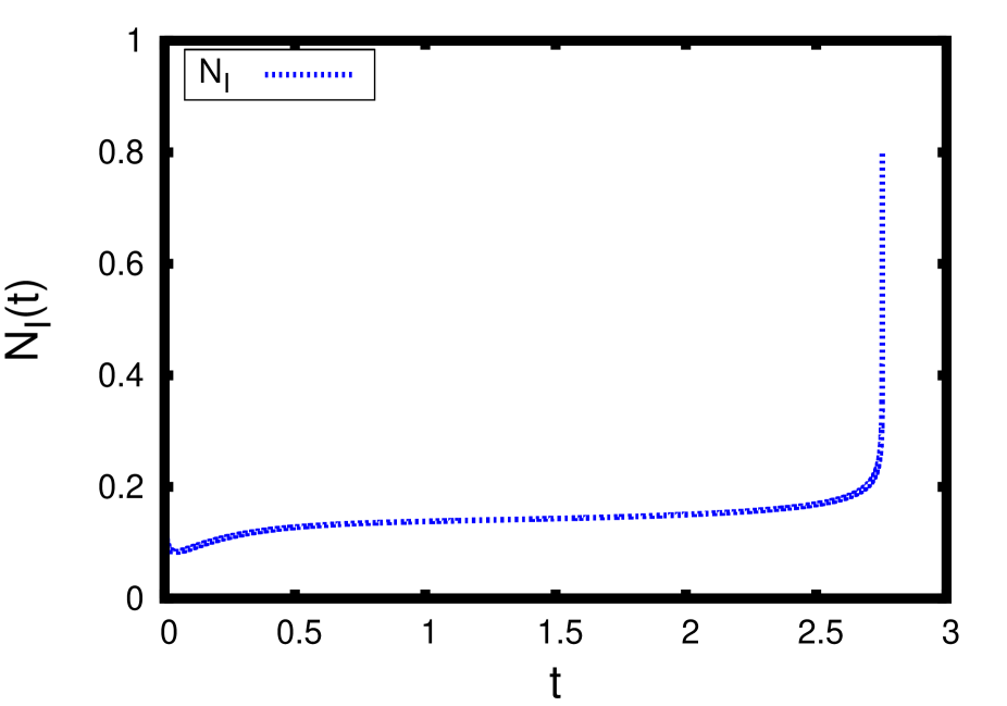
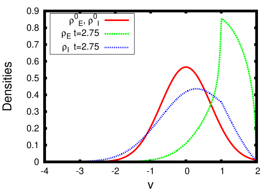
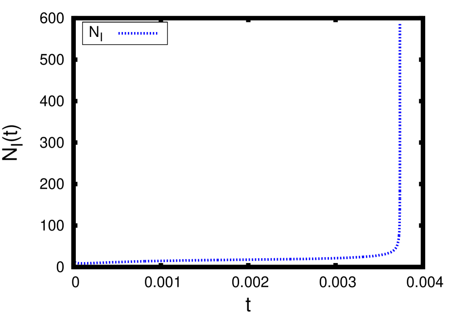
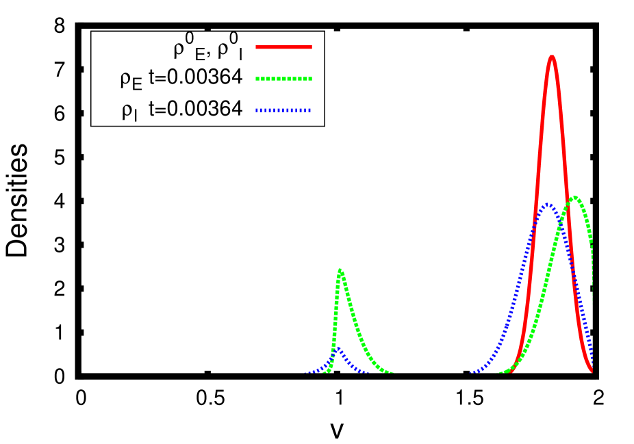
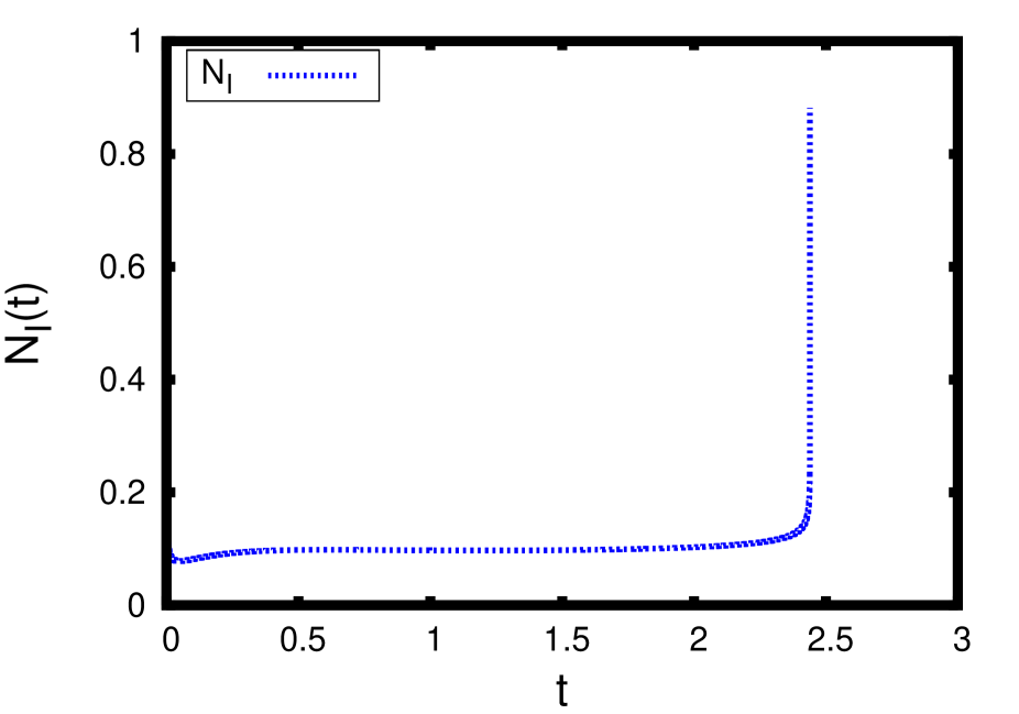
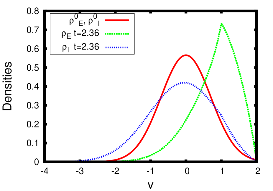
Theorem 3.1 shows that blow-up occurs when the connectivity parameter of the excitatory to excitatory synapses, bEEsuperscriptsubscript𝑏𝐸𝐸b_{E}^{E}, is large enough or if initially there are many excitatory neurons with a voltage value of their membrane potential very close to the threshold value, VFsubscript𝑉𝐹V_{F}. From a biological perspective, and in view of the numerical results in Section 5 (Figs. 3, 4 and 5), in the first case, blow-up appears due to the strong influence of the excitatory population on the behavior of the network, poducing the incontrolled growth of the firing rate at finite time. In the second case, even with small connectivity parameter bEEsuperscriptsubscript𝑏𝐸𝐸b_{E}^{E}, the abundance of excitatory neurons with membrane potential voltage values sufficiently close to VFsubscript𝑉𝐹V_{F} causes the firing rate to diverge in finite time. For a microscopic description, at the level of individual neurons, we refer to [12] and [13] where the blow-up phenomenon is also analysed.

As mentioned above it was proved in [7] that fully excitatory networks can blow-up in finite time, when one includes the refractory state. This result can be extended to the case of excitatory-inhibitory networks by following the same ideas of Theorem 3.1.

4 Steady states and long time behavior

4.1 Steady states

For excitatory and inhibitory networks, the study of their steady states follows a similar strategy to that for the fully excitatory or inhibitory cases. However, for coupled networks the system solved by the stationary solutions is much more complicate, as we will see throughout this section.

As in [5], let us search for continuous stationary solutions (ρE,ρI)subscript𝜌𝐸subscript𝜌𝐼(\rho_{E},\rho_{I}) of (2.8) such that ρE,ρIsubscript𝜌𝐸subscript𝜌𝐼\rho_{E},\ \rho_{I} are C1superscript𝐶1C^{1} regular, except possibly at V=VR𝑉subscript𝑉𝑅V=V_{R} where they are Lipschitz, and satisfy the following identity:

v[hα(v)ρα(v)aα(NE,NI)ραv(v)NαH(vVR)]=0,α=E,I,formulae-sequence𝑣delimited-[]superscript𝛼𝑣subscript𝜌𝛼𝑣subscript𝑎𝛼subscript𝑁𝐸subscript𝑁𝐼subscript𝜌𝛼𝑣𝑣subscript𝑁𝛼𝐻𝑣subscript𝑉𝑅0𝛼𝐸𝐼\frac{\partial}{\partial v}[h^{\alpha}(v)\rho_{\alpha}(v)-a_{\alpha}(N_{E},N_{I})\frac{\partial\rho_{\alpha}}{\partial v}(v)-N_{\alpha}H(v-V_{R})]=0,\quad\alpha=E,I,

in the sense of distributions, where H𝐻H denotes the Heaviside function. Considering hα(v,NE,NI)=V0α(NE,NI)vsuperscript𝛼𝑣subscript𝑁𝐸subscript𝑁𝐼superscriptsubscript𝑉0𝛼subscript𝑁𝐸subscript𝑁𝐼𝑣h^{\alpha}(v,N_{E},N_{I})=V_{0}^{\alpha}(N_{E},N_{I})-v, with V0α(NE,NI)=bEαNEbIαNI+(bEαbEE)νE,extsuperscriptsubscript𝑉0𝛼subscript𝑁𝐸subscript𝑁𝐼superscriptsubscript𝑏𝐸𝛼subscript𝑁𝐸superscriptsubscript𝑏𝐼𝛼subscript𝑁𝐼superscriptsubscript𝑏𝐸𝛼superscriptsubscript𝑏𝐸𝐸subscript𝜈𝐸𝑒𝑥𝑡V_{0}^{\alpha}(N_{E},N_{I})=b_{E}^{\alpha}N_{E}-b_{I}^{\alpha}N_{I}+(b_{E}^{\alpha}-b_{E}^{E})\nu_{E,ext}, the definition of Nαsubscript𝑁𝛼N_{\alpha} in (2.12) and the Dirichlet boundary conditions in (2.9), we find the following initial value problem for every α=E,I𝛼𝐸𝐼\alpha=E,I:

{ραv(v)=V0α(NE,NI)vaα(NE,NI)ρα(v)NαH(vVR)aα(NE,NI),ρα(VF)=0,casessubscript𝜌𝛼𝑣𝑣superscriptsubscript𝑉0𝛼subscript𝑁𝐸subscript𝑁𝐼𝑣subscript𝑎𝛼subscript𝑁𝐸subscript𝑁𝐼subscript𝜌𝛼𝑣subscript𝑁𝛼𝐻𝑣subscript𝑉𝑅subscript𝑎𝛼subscript𝑁𝐸subscript𝑁𝐼subscript𝜌𝛼subscript𝑉𝐹0\left\{\begin{array}[]{l}\frac{\partial\rho_{\alpha}}{\partial v}(v)=\frac{V_{0}^{\alpha}(N_{E},N_{I})-v}{a_{\alpha}(N_{E},N_{I})}\rho_{\alpha}(v)-\frac{N_{\alpha}H(v-V_{R})}{a_{\alpha}(N_{E},N_{I})},\\ \rho_{\alpha}(V_{F})=0,\end{array}\right.

whose solutions are of the form

ρα(v)=Nαaα(NE,NI)e(vV0α(NE,NI))22aα(NE,NI)max(v,VR)VFe(wV0α(NE,NI))22aα(NE,NI)𝑑w,α=E,I.formulae-sequencesubscript𝜌𝛼𝑣subscript𝑁𝛼subscript𝑎𝛼subscript𝑁𝐸subscript𝑁𝐼superscript𝑒superscript𝑣superscriptsubscript𝑉0𝛼subscript𝑁𝐸subscript𝑁𝐼22subscript𝑎𝛼subscript𝑁𝐸subscript𝑁𝐼superscriptsubscript𝑣subscript𝑉𝑅subscript𝑉𝐹superscript𝑒superscript𝑤superscriptsubscript𝑉0𝛼subscript𝑁𝐸subscript𝑁𝐼22subscript𝑎𝛼subscript𝑁𝐸subscript𝑁𝐼differential-d𝑤𝛼𝐸𝐼\rho_{\alpha}(v)=\frac{N_{\alpha}}{a_{\alpha}(N_{E},N_{I})}e^{-\frac{(v-V_{0}^{\alpha}(N_{E},N_{I}))^{2}}{2a_{\alpha}(N_{E},N_{I})}}\int_{\max(v,V_{R})}^{V_{F}}e^{\frac{(w-V_{0}^{\alpha}(N_{E},N_{I}))^{2}}{2a_{\alpha}(N_{E},N_{I})}}dw,\quad\alpha=E,I. (4.1)

The expression (4.1) is not an explicit formula for ραsubscript𝜌𝛼\rho_{\alpha}, since the right hand side depends on Nαsubscript𝑁𝛼N_{\alpha}, but provides a system of implicit equations for Nαsubscript𝑁𝛼N_{\alpha}

aα(NE,NI)Nα=VFe(vV0α(NE,NI))22aα(NE,NI)[max(v,VR)VFe(wV0α(NE,NI))22aα(NE,NI)𝑑w]𝑑v,α=E,I,formulae-sequencesubscript𝑎𝛼subscript𝑁𝐸subscript𝑁𝐼subscript𝑁𝛼superscriptsubscriptsubscript𝑉𝐹superscript𝑒superscript𝑣superscriptsubscript𝑉0𝛼subscript𝑁𝐸subscript𝑁𝐼22subscript𝑎𝛼subscript𝑁𝐸subscript𝑁𝐼delimited-[]superscriptsubscript𝑣subscript𝑉𝑅subscript𝑉𝐹superscript𝑒superscript𝑤superscriptsubscript𝑉0𝛼subscript𝑁𝐸subscript𝑁𝐼22subscript𝑎𝛼subscript𝑁𝐸subscript𝑁𝐼differential-d𝑤differential-d𝑣𝛼𝐸𝐼\frac{a_{\alpha}(N_{E},N_{I})}{N_{\alpha}}=\int_{-\infty}^{V_{F}}e^{-\frac{(v-V_{0}^{\alpha}(N_{E},N_{I}))^{2}}{2a_{\alpha}(N_{E},N_{I})}}\left[\int_{\max{(v,V_{R})}}^{V_{F}}e^{\frac{(w-V_{0}^{\alpha}(N_{E},N_{I}))^{2}}{2a_{\alpha}(N_{E},N_{I})}}dw\right]dv,\qquad\alpha=E,I, (4.2)

for which the conservation of mass (VFρα(v,t)𝑑v=1superscriptsubscriptsubscript𝑉𝐹subscript𝜌𝛼𝑣𝑡differential-d𝑣1\int_{-\infty}^{V_{F}}\rho_{\alpha}(v,t)dv=1) has been used. Therefore, the stationary solutions (ρE,ρI)subscript𝜌𝐸subscript𝜌𝐼(\rho_{E},\rho_{I}) have the profile (4.1), where (NE,NI)subscript𝑁𝐸subscript𝑁𝐼(N_{E},N_{I}) are positive solutions of the implicit system (4.2), and there are as many as solutions of (4.2). Of course, in the particular case of a linear system, that is V0α(NE,NI)=0superscriptsubscript𝑉0𝛼subscript𝑁𝐸subscript𝑁𝐼0V_{0}^{\alpha}(N_{E},N_{I})=0 and aα(NE,NI)subscript𝑎𝛼subscript𝑁𝐸subscript𝑁𝐼a_{\alpha}(N_{E},N_{I}) independent of the firing rates, there is a unique steady state.

Determining the number of solutions of the implicit system (4.2) is a difficult task. In this section we find some conditions on the parameters of the model in order to reach this goal. Firstly, we consider the following change of variables and notation:

z𝑧\displaystyle z =\displaystyle\!\!\!\!\!=\!\!\!\!\! vV0E(NE,NI)aE(NE,NI),u=wV0E(NE,NI)aE(NE,NI),wF:=VFV0E(NE,NI)aE(NE,NI),wR:=VRV0E(NE,NI)aE(NE,NI),formulae-sequence𝑣superscriptsubscript𝑉0𝐸subscript𝑁𝐸subscript𝑁𝐼subscript𝑎𝐸subscript𝑁𝐸subscript𝑁𝐼𝑢𝑤superscriptsubscript𝑉0𝐸subscript𝑁𝐸subscript𝑁𝐼subscript𝑎𝐸subscript𝑁𝐸subscript𝑁𝐼formulae-sequenceassignsubscript𝑤𝐹subscript𝑉𝐹superscriptsubscript𝑉0𝐸subscript𝑁𝐸subscript𝑁𝐼subscript𝑎𝐸subscript𝑁𝐸subscript𝑁𝐼assignsubscript𝑤𝑅subscript𝑉𝑅superscriptsubscript𝑉0𝐸subscript𝑁𝐸subscript𝑁𝐼subscript𝑎𝐸subscript𝑁𝐸subscript𝑁𝐼\displaystyle\frac{v-V_{0}^{E}(N_{E},N_{I})}{\sqrt{a_{E}(N_{E},N_{I})}},\ u=\frac{w-V_{0}^{E}(N_{E},N_{I})}{\sqrt{a_{E}(N_{E},N_{I})}},\ w_{F}:=\frac{V_{F}-V_{0}^{E}(N_{E},N_{I})}{\sqrt{a_{E}(N_{E},N_{I})}},\ w_{R}:=\frac{V_{R}-V_{0}^{E}(N_{E},N_{I})}{\sqrt{a_{E}(N_{E},N_{I})}},
z~~𝑧\displaystyle\tilde{z} =\displaystyle\!\!\!\!\!=\!\!\!\!\! vV0I(NE,NI)aI(NE,NI),u~=wV0I(NE,NI)aI(NE,NI),w~F:=VFV0I(NE,NI)aI(NE,NI),w~R:=VRV0I(NE,NI)aI(NE,NI).formulae-sequence𝑣superscriptsubscript𝑉0𝐼subscript𝑁𝐸subscript𝑁𝐼subscript𝑎𝐼subscript𝑁𝐸subscript𝑁𝐼~𝑢𝑤superscriptsubscript𝑉0𝐼subscript𝑁𝐸subscript𝑁𝐼subscript𝑎𝐼subscript𝑁𝐸subscript𝑁𝐼formulae-sequenceassignsubscript~𝑤𝐹subscript𝑉𝐹superscriptsubscript𝑉0𝐼subscript𝑁𝐸subscript𝑁𝐼subscript𝑎𝐼subscript𝑁𝐸subscript𝑁𝐼assignsubscript~𝑤𝑅subscript𝑉𝑅superscriptsubscript𝑉0𝐼subscript𝑁𝐸subscript𝑁𝐼subscript𝑎𝐼subscript𝑁𝐸subscript𝑁𝐼\displaystyle\frac{v-V_{0}^{I}(N_{E},N_{I})}{\sqrt{a_{I}(N_{E},N_{I})}},\ \tilde{u}=\frac{w-V_{0}^{I}(N_{E},N_{I})}{\sqrt{a_{I}(N_{E},N_{I})}},\ \tilde{w}_{F}:=\frac{V_{F}-V_{0}^{I}(N_{E},N_{I})}{\sqrt{a_{I}(N_{E},N_{I})}},\ \tilde{w}_{R}:=\frac{V_{R}-V_{0}^{I}(N_{E},N_{I})}{\sqrt{a_{I}(N_{E},N_{I})}}.

With these new variables, the system (4.2) is rewritten as

1NE1subscript𝑁𝐸\displaystyle\frac{1}{N_{E}} =\displaystyle= I1(NE,NI),whereI1(NE,NI)=wFez22max(z,wR)wFeu22𝑑u𝑑z,subscript𝐼1subscript𝑁𝐸subscript𝑁𝐼wheresubscript𝐼1subscript𝑁𝐸subscript𝑁𝐼superscriptsubscriptsubscript𝑤𝐹superscript𝑒superscript𝑧22superscriptsubscript𝑧subscript𝑤𝑅subscript𝑤𝐹superscript𝑒superscript𝑢22differential-d𝑢differential-d𝑧\displaystyle I_{1}(N_{E},N_{I}),\ \mbox{where}\ I_{1}(N_{E},N_{I})=\int_{-\infty}^{w_{F}}e^{-\frac{z^{2}}{2}}\int_{\max(z,w_{R})}^{w_{F}}e^{\frac{u^{2}}{2}}du\ dz,
1NI1subscript𝑁𝐼\displaystyle\frac{1}{N_{I}} =\displaystyle= I2(NE,NI),whereI2(NE,NI)=w~Fez22max(z,w~R)w~Feu22𝑑u𝑑z.subscript𝐼2subscript𝑁𝐸subscript𝑁𝐼wheresubscript𝐼2subscript𝑁𝐸subscript𝑁𝐼superscriptsubscriptsubscript~𝑤𝐹superscript𝑒superscript𝑧22superscriptsubscript𝑧subscript~𝑤𝑅subscript~𝑤𝐹superscript𝑒superscript𝑢22differential-d𝑢differential-d𝑧\displaystyle I_{2}(N_{E},N_{I}),\ \mbox{where}\ I_{2}(N_{E},N_{I})=\int_{-\infty}^{\tilde{w}_{F}}e^{-\frac{z^{2}}{2}}\int_{\max(z,\tilde{w}_{R})}^{\tilde{w}_{F}}e^{\frac{u^{2}}{2}}du\ dz. (4.3)

Now, using s=zu2𝑠𝑧𝑢2s=\frac{z-u}{2} and s~=z+u2~𝑠𝑧𝑢2\tilde{s}=\frac{z+u}{2}, the functions I1subscript𝐼1I_{1} and I2subscript𝐼2I_{2} can be formulated as

I1(NE,NI)=0es22s(eswFeswR)𝑑s,subscript𝐼1subscript𝑁𝐸subscript𝑁𝐼superscriptsubscript0superscript𝑒superscript𝑠22𝑠superscript𝑒𝑠subscript𝑤𝐹superscript𝑒𝑠subscript𝑤𝑅differential-d𝑠\displaystyle I_{1}(N_{E},N_{I})=\int_{0}^{\infty}\frac{e^{-\frac{s^{2}}{2}}}{s}(e^{s\,w_{F}}-e^{s\,w_{R}})\ ds,
I2(NE,NI)=0es22s(esw~Fesw~R)𝑑s.subscript𝐼2subscript𝑁𝐸subscript𝑁𝐼superscriptsubscript0superscript𝑒superscript𝑠22𝑠superscript𝑒𝑠subscript~𝑤𝐹superscript𝑒𝑠subscript~𝑤𝑅differential-d𝑠\displaystyle I_{2}(N_{E},N_{I})=\int_{0}^{\infty}\frac{e^{-\frac{s^{2}}{2}}}{s}(e^{s\,\tilde{w}_{F}}-e^{s\,\tilde{w}_{R}})\ ds.

When bIE=bEI=0superscriptsubscript𝑏𝐼𝐸superscriptsubscript𝑏𝐸𝐼0b_{I}^{E}=b_{E}^{I}=0 the equations are uncoupled and the number of steady states can be determined in the same way as in [5], depending on the values of bEEsuperscriptsubscript𝑏𝐸𝐸b_{E}^{E}, since for the inhibitory equation there is always a unique steady state. The following theorem establishes a classification of the number of steady states in terms of the model parameters, in the case that the connectivity parameters bIEsuperscriptsubscript𝑏𝐼𝐸b_{I}^{E} and bEIsuperscriptsubscript𝑏𝐸𝐼b_{E}^{I} do not vanish, and in comparison with the values of the pure connectivity parameters bEEsuperscriptsubscript𝑏𝐸𝐸b_{E}^{E} and bIIsuperscriptsubscript𝑏𝐼𝐼b_{I}^{I}.

Theorem 4.1

Assume that the connectivity parameters bIEsuperscriptsubscript𝑏𝐼𝐸b_{I}^{E} and bEIsuperscriptsubscript𝑏𝐸𝐼b_{E}^{I} do not vanish (bIE,bEI>0superscriptsubscript𝑏𝐼𝐸superscriptsubscript𝑏𝐸𝐼0b_{I}^{E},\,b_{E}^{I}>0), aαsubscript𝑎𝛼a_{\alpha} is independent of NEsubscript𝑁𝐸N_{E} and NIsubscript𝑁𝐼N_{I}, aα(NE,NI)=aαsubscript𝑎𝛼subscript𝑁𝐸subscript𝑁𝐼subscript𝑎𝛼a_{\alpha}(N_{E},N_{I})=a_{\alpha}, and hα(v,NE,NI)=V0α(NE,NI)vsuperscript𝛼𝑣subscript𝑁𝐸subscript𝑁𝐼superscriptsubscript𝑉0𝛼subscript𝑁𝐸subscript𝑁𝐼𝑣h^{\alpha}(v,N_{E},N_{I})=V_{0}^{\alpha}(N_{E},N_{I})-v with V0α(NE,NI)=bEαNEbIαNI+(bEαbEE)νE,extsuperscriptsubscript𝑉0𝛼subscript𝑁𝐸subscript𝑁𝐼superscriptsubscript𝑏𝐸𝛼subscript𝑁𝐸superscriptsubscript𝑏𝐼𝛼subscript𝑁𝐼superscriptsubscript𝑏𝐸𝛼superscriptsubscript𝑏𝐸𝐸subscript𝜈𝐸𝑒𝑥𝑡V_{0}^{\alpha}(N_{E},N_{I})=b_{E}^{\alpha}N_{E}-b_{I}^{\alpha}N_{I}+(b_{E}^{\alpha}-b_{E}^{E})\nu_{E,ext} for all α=E,I𝛼𝐸𝐼\alpha=E,I. Then:

  1. 1.

    There is an even number of steady states or there are no steady states for (2.8)-(2.12) if

    (VFVR)2<(VFVR)(bEEbII)+bEEbIIbIEbEI.superscriptsubscript𝑉𝐹subscript𝑉𝑅2subscript𝑉𝐹subscript𝑉𝑅superscriptsubscript𝑏𝐸𝐸superscriptsubscript𝑏𝐼𝐼superscriptsubscript𝑏𝐸𝐸superscriptsubscript𝑏𝐼𝐼superscriptsubscript𝑏𝐼𝐸superscriptsubscript𝑏𝐸𝐼(V_{F}-V_{R})^{2}<(V_{F}-V_{R})(b_{E}^{E}-b_{I}^{I})+b_{E}^{E}b_{I}^{I}-b_{I}^{E}b_{E}^{I}. (4.4)

    If bEEsuperscriptsubscript𝑏𝐸𝐸b_{E}^{E} is large enough in comparison with the rest of connectivity parameters, there are no steady states. Specifically, there are no steady states if both (4.4) and

    max{I1(0)2(VF+bIENI(N¯E)),bEIbIEbII,2(VFVR)}<bEEsubscript𝐼102subscript𝑉𝐹superscriptsubscript𝑏𝐼𝐸subscript𝑁𝐼subscript¯𝑁𝐸superscriptsubscript𝑏𝐸𝐼superscriptsubscript𝑏𝐼𝐸superscriptsubscript𝑏𝐼𝐼2subscript𝑉𝐹subscript𝑉𝑅superscriptsubscript𝑏𝐸𝐸\max\left\{I_{1}(0)2\left(V_{F}+b_{I}^{E}N_{I}(\bar{N}_{E})\right),\frac{b_{E}^{I}b_{I}^{E}}{b_{I}^{I}},2(V_{F}-V_{R})\right\}<b_{E}^{E} (4.5)

    are fulfilled, where

    N¯E=max{NE0:NE=2(bEINI(NE)+VF)bEE}.subscript¯𝑁𝐸:superscriptsubscript𝑁𝐸0superscriptsubscript𝑁𝐸2superscriptsubscript𝑏𝐸𝐼subscript𝑁𝐼superscriptsubscript𝑁𝐸subscript𝑉𝐹superscriptsubscript𝑏𝐸𝐸\bar{N}_{E}=\max\left\{N_{E}^{*}\geq 0:N_{E}^{*}=\frac{2(b_{E}^{I}N_{I}(N_{E}^{*})+V_{F})}{b_{E}^{E}}\right\}. (4.6)
  2. 2.

    There is an odd number of steady states for (2.8)-(2.12) if

    (VFVR)(bEEbII)+bEEbIIbIEbEI<(VFVR)2.subscript𝑉𝐹subscript𝑉𝑅superscriptsubscript𝑏𝐸𝐸superscriptsubscript𝑏𝐼𝐼superscriptsubscript𝑏𝐸𝐸superscriptsubscript𝑏𝐼𝐼superscriptsubscript𝑏𝐼𝐸superscriptsubscript𝑏𝐸𝐼superscriptsubscript𝑉𝐹subscript𝑉𝑅2(V_{F}-V_{R})(b_{E}^{E}-b_{I}^{I})+b_{E}^{E}b_{I}^{I}-b_{I}^{E}b_{E}^{I}<(V_{F}-V_{R})^{2}. (4.7)

    If bEEsuperscriptsubscript𝑏𝐸𝐸b_{E}^{E} is small enough in comparison with the rest of connectivity parameters, there is a unique steady state.

Proof. The proof reduces to study the existence of solutions to (4.3). It is organized in several steps.

Step 1. To prove that 1NI=I2(NE,NI)1subscript𝑁𝐼subscript𝐼2subscript𝑁𝐸subscript𝑁𝐼\frac{1}{N_{I}}=I_{2}(N_{E},N_{I}) admits a unique solution NI(NE)subscript𝑁𝐼subscript𝑁𝐸N_{I}(N_{E}) for NEsubscript𝑁𝐸N_{E} fixed.

Given NE[0,)subscript𝑁𝐸0N_{E}\in[0,\infty) and following analogous ideas as in [5], it is easy to observe that there is a unique solution NI(NE)subscript𝑁𝐼subscript𝑁𝐸N_{I}(N_{E}) to

1NI=I2(NE,NI).1subscript𝑁𝐼subscript𝐼2subscript𝑁𝐸subscript𝑁𝐼\displaystyle\frac{1}{N_{I}}=I_{2}(N_{E},N_{I}). (4.8)

This fact is a consequence of the following properties of I2subscript𝐼2I_{2}:

  1. 1.

    I2(NE,NI)subscript𝐼2subscript𝑁𝐸subscript𝑁𝐼I_{2}(N_{E},N_{I}) is Csuperscript𝐶C^{\infty} in both variables.

  2. 2.

    For every NEsubscript𝑁𝐸N_{E} fixed, I2(NE,NI)subscript𝐼2subscript𝑁𝐸subscript𝑁𝐼I_{2}(N_{E},N_{I}) is an increasing strictly convex function on NIsubscript𝑁𝐼N_{I}, since for all integers k1𝑘1k\geq 1

    kI2NIk=(bIIaI)k0es22sk1(esw~Fesw~R)𝑑s.superscript𝑘subscript𝐼2superscriptsubscript𝑁𝐼𝑘superscriptsuperscriptsubscript𝑏𝐼𝐼subscript𝑎𝐼𝑘superscriptsubscript0superscript𝑒superscript𝑠22superscript𝑠𝑘1superscript𝑒𝑠subscript~𝑤𝐹superscript𝑒𝑠subscript~𝑤𝑅differential-d𝑠\frac{\partial^{k}I_{2}}{\partial N_{I}^{k}}=\left(\frac{b_{I}^{I}}{\sqrt{a_{I}}}\right)^{k}\int_{0}^{\infty}e^{-\frac{{s}^{2}}{2}}s^{k-1}(e^{s\tilde{w}_{F}}-e^{s\tilde{w}_{R}})\ ds. (4.9)

    Thus, limNII2(NE,NI)=subscriptsubscript𝑁𝐼subscript𝐼2subscript𝑁𝐸subscript𝑁𝐼\displaystyle\lim_{N_{I}\rightarrow\infty}I_{2}(N_{E},N_{I})=\infty for every NEsubscript𝑁𝐸N_{E} fixed.

  3. 3.

    If we consider NI[0,)subscript𝑁𝐼0N_{I}\in[0,\infty), I2(NE,NI)subscript𝐼2subscript𝑁𝐸subscript𝑁𝐼I_{2}(N_{E},N_{I}) is a decreasing convex function on NEsubscript𝑁𝐸N_{E}, since for all integers k1𝑘1k\geq 1

    kI2NEk=(1)k(bEIaI)k0es22sk1(esw~Fesw~R)𝑑s.superscript𝑘subscript𝐼2superscriptsubscript𝑁𝐸𝑘superscript1𝑘superscriptsuperscriptsubscript𝑏𝐸𝐼subscript𝑎𝐼𝑘superscriptsubscript0superscript𝑒superscript𝑠22superscript𝑠𝑘1superscript𝑒𝑠subscript~𝑤𝐹superscript𝑒𝑠subscript~𝑤𝑅differential-d𝑠\frac{\partial^{k}I_{2}}{\partial N_{E}^{k}}=(-1)^{k}\left(\frac{b_{E}^{I}}{\sqrt{a_{I}}}\right)^{k}\int_{0}^{\infty}e^{-\frac{{s}^{2}}{2}}s^{k-1}(e^{s\tilde{w}_{F}}-e^{s\tilde{w}_{R}})\ ds. (4.10)

    Thus, limNEI2(NE,NI)=0subscriptsubscript𝑁𝐸subscript𝐼2subscript𝑁𝐸subscript𝑁𝐼0\displaystyle\lim_{N_{E}\rightarrow\infty}I_{2}(N_{E},N_{I})=0, for every NIsubscript𝑁𝐼N_{I} fixed.

  4. 4.

    Using expression (4.3) for I2subscript𝐼2I_{2}, we have I2(NE,0)<subscript𝐼2subscript𝑁𝐸0I_{2}(N_{E},0)<\infty, for every NEsubscript𝑁𝐸N_{E} fixed, since

    I2(NE,0)=w~F(0)ez22max(z,w~R(0))w~F(0)eu22𝑑u𝑑z2π(VFVRaI)em2aI,subscript𝐼2subscript𝑁𝐸0superscriptsubscriptsubscript~𝑤𝐹0superscript𝑒superscript𝑧22superscriptsubscript𝑧subscript~𝑤𝑅0subscript~𝑤𝐹0superscript𝑒superscript𝑢22differential-d𝑢differential-d𝑧2𝜋subscript𝑉𝐹subscript𝑉𝑅subscript𝑎𝐼superscript𝑒𝑚2subscript𝑎𝐼I_{2}(N_{E},0)=\int_{-\infty}^{\tilde{w}_{F}(0)}e^{-\frac{z^{2}}{2}}\int_{\max(z,\tilde{w}_{R}(0))}^{\tilde{w}_{F}(0)}e^{\frac{u^{2}}{2}}\,du\,dz\leq\sqrt{2\pi}\left(\frac{V_{F}-V_{R}}{\sqrt{a_{I}}}\right)e^{\frac{m}{2a_{I}}},

    where m=max{(VFbEINE(bEIbEE)νE,ext)2,(VRbEINE(bEIbEE)νE,ext)2}𝑚superscriptsubscript𝑉𝐹superscriptsubscript𝑏𝐸𝐼subscript𝑁𝐸superscriptsubscript𝑏𝐸𝐼superscriptsubscript𝑏𝐸𝐸subscript𝜈𝐸𝑒𝑥𝑡2superscriptsubscript𝑉𝑅superscriptsubscript𝑏𝐸𝐼subscript𝑁𝐸superscriptsubscript𝑏𝐸𝐼superscriptsubscript𝑏𝐸𝐸subscript𝜈𝐸𝑒𝑥𝑡2m=\max\{(V_{F}-b_{E}^{I}N_{E}-(b_{E}^{I}-b_{E}^{E})\nu_{E,ext})^{2},(V_{R}-b_{E}^{I}N_{E}-(b_{E}^{I}-b_{E}^{E})\nu_{E,ext})^{2}\}.

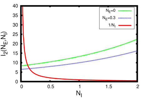
Figure 1 depicts the function I2subscript𝐼2I_{2} in terms of NIsubscript𝑁𝐼N_{I} for different values of NEsubscript𝑁𝐸N_{E} fixed. In this figure, the properties of I2subscript𝐼2I_{2} enumerated above can be observed.

Refer to caption
Figure 1: The function I2subscript𝐼2I_{2} in terms of NIsubscript𝑁𝐼N_{I}, for different values of NEsubscript𝑁𝐸N_{E} fixed. I2subscript𝐼2I_{2} is an increasing function on NIsubscript𝑁𝐼N_{I} and decreasing on NEsubscript𝑁𝐸N_{E}.

Step 2. Properties of NI(NE)subscript𝑁𝐼subscript𝑁𝐸N_{I}(N_{E}).

Obtaining an analytical expression of NI(NE)subscript𝑁𝐼subscript𝑁𝐸N_{I}(N_{E}) is not easy. However, some properties of NI(NE)subscript𝑁𝐼subscript𝑁𝐸N_{I}(N_{E}) are enough to prove the theorem:

  1. 1.

    NI(NE)>0subscript𝑁𝐼subscript𝑁𝐸0N_{I}(N_{E})>0, for-all\forall NE[0,)subscript𝑁𝐸0N_{E}\in[0,\infty).

  2. 2.

    NI(NE)subscript𝑁𝐼subscript𝑁𝐸N_{I}(N_{E}) is an increasing function, NE[0,)for-allsubscript𝑁𝐸0\forall\ N_{E}\in[0,\infty), since

    NI(NE)=NI2(NE)I2NE(NE,NI(NE))1+NI2(NE)I2NI(NE,NI(NE))superscriptsubscript𝑁𝐼subscript𝑁𝐸superscriptsubscript𝑁𝐼2subscript𝑁𝐸subscript𝐼2subscript𝑁𝐸subscript𝑁𝐸subscript𝑁𝐼subscript𝑁𝐸1superscriptsubscript𝑁𝐼2subscript𝑁𝐸subscript𝐼2subscript𝑁𝐼subscript𝑁𝐸subscript𝑁𝐼subscript𝑁𝐸N_{I}^{\prime}(N_{E})=\frac{-N_{I}^{2}(N_{E})\frac{\partial I_{2}}{\partial N_{E}}(N_{E},N_{I}(N_{E}))}{1+N_{I}^{2}(N_{E})\frac{\partial I_{2}}{\partial N_{I}}(N_{E},N_{I}(N_{E}))} (4.11)

    is nonnegative. Expression (4.11) is obtained by differentiating NI(NE)I2(NE,NI(NE))=1subscript𝑁𝐼subscript𝑁𝐸subscript𝐼2subscript𝑁𝐸subscript𝑁𝐼subscript𝑁𝐸1N_{I}(N_{E})I_{2}(N_{E},N_{I}(N_{E}))=1 with respect to NEsubscript𝑁𝐸N_{E}.

  3. 3.

    limNENI(NE)=subscriptsubscript𝑁𝐸subscript𝑁𝐼subscript𝑁𝐸\displaystyle\lim_{N_{E}\rightarrow\infty}N_{I}(N_{E})=\infty, because NI(NE)subscript𝑁𝐼subscript𝑁𝐸N_{I}(N_{E}) is a positive increasing function, thus its limit could be infinite or a constant C>0𝐶0C>0. The finite limit leads to a contradiction since 1NI(NE)=I2(NE,NI(NE))1subscript𝑁𝐼subscript𝑁𝐸subscript𝐼2subscript𝑁𝐸subscript𝑁𝐼subscript𝑁𝐸\frac{1}{N_{I}(N_{E})}=I_{2}(N_{E},N_{I}(N_{E})), and then limNE1NI(NE)=1Csubscriptsubscript𝑁𝐸1subscript𝑁𝐼subscript𝑁𝐸1𝐶\displaystyle\lim_{N_{E}\rightarrow\infty}\frac{1}{N_{I}(N_{E})}=\frac{1}{C}, while limNEI2(NE,NI(NE))=0subscriptsubscript𝑁𝐸subscript𝐼2subscript𝑁𝐸subscript𝑁𝐼subscript𝑁𝐸0\displaystyle\lim_{N_{E}\rightarrow\infty}I_{2}(N_{E},N_{I}(N_{E}))=0 because limNEI2(NE,C)=0subscriptsubscript𝑁𝐸subscript𝐼2subscript𝑁𝐸𝐶0\displaystyle\lim_{N_{E}\to\infty}I_{2}(N_{E},C)=0.

  4. 4.

    0<NI(NE)<bEIbII0subscriptsuperscript𝑁𝐼subscript𝑁𝐸superscriptsubscript𝑏𝐸𝐼superscriptsubscript𝑏𝐼𝐼0<N^{\prime}_{I}(N_{E})<\frac{b_{E}^{I}}{b_{I}^{I}}. It is a consequence of the fact that

    NI(NE)=bEINI2(NE)I(NE)aI+bIINI2(NE)I(NE),superscriptsubscript𝑁𝐼subscript𝑁𝐸superscriptsubscript𝑏𝐸𝐼superscriptsubscript𝑁𝐼2subscript𝑁𝐸𝐼subscript𝑁𝐸subscript𝑎𝐼superscriptsubscript𝑏𝐼𝐼superscriptsubscript𝑁𝐼2subscript𝑁𝐸𝐼subscript𝑁𝐸N_{I}^{\prime}(N_{E})=\frac{b_{E}^{I}N_{I}^{2}(N_{E})I(N_{E})}{\sqrt{a_{I}}+b_{I}^{I}N_{I}^{2}(N_{E})I(N_{E})}, (4.12)

    where I(NE)=0es2/2e(bEINEbIINI(NE)+(bEIbEE)νE,ext)saI(esVF/aIesVR/aI)𝑑s.𝐼subscript𝑁𝐸superscriptsubscript0superscript𝑒superscript𝑠22superscript𝑒superscriptsubscript𝑏𝐸𝐼subscript𝑁𝐸superscriptsubscript𝑏𝐼𝐼subscript𝑁𝐼subscript𝑁𝐸superscriptsubscript𝑏𝐸𝐼superscriptsubscript𝑏𝐸𝐸subscript𝜈𝐸𝑒𝑥𝑡𝑠subscript𝑎𝐼superscript𝑒𝑠subscript𝑉𝐹subscript𝑎𝐼superscript𝑒𝑠subscript𝑉𝑅subscript𝑎𝐼differential-d𝑠I(N_{E})=\int_{0}^{\infty}e^{-s^{2}/2}e^{\frac{-(b_{E}^{I}N_{E}-b_{I}^{I}N_{I}(N_{E})+(b_{E}^{I}-b_{E}^{E})\nu_{E,ext})s}{\sqrt{a_{I}}}}\left(e^{sV_{F}/\sqrt{a_{I}}}-e^{sV_{R}/\sqrt{a_{I}}}\right)\ ds.

    Expression (4.12) is obtained using (4.9), (4.10), (4.11) and the definition of w~Fsubscript~𝑤𝐹\tilde{w}_{F} and w~Rsubscript~𝑤𝑅\tilde{w}_{R}.

  5. 5.

    limNENI(NE)=bEILaI+bIILsubscriptsubscript𝑁𝐸superscriptsubscript𝑁𝐼subscript𝑁𝐸superscriptsubscript𝑏𝐸𝐼𝐿subscript𝑎𝐼superscriptsubscript𝑏𝐼𝐼𝐿\displaystyle\lim_{N_{E}\to\infty}N_{I}^{\prime}(N_{E})=\frac{b_{E}^{I}L}{\sqrt{a_{I}}+b_{I}^{I}\,L}, where limNENI2(NE)I(NE)=Lsubscriptsubscript𝑁𝐸superscriptsubscript𝑁𝐼2subscript𝑁𝐸𝐼subscript𝑁𝐸𝐿\displaystyle\lim_{N_{E}\to\infty}N_{I}^{2}(N_{E})I(N_{E})=L.

  6. 6.

    L=aIVFVR𝐿subscript𝑎𝐼subscript𝑉𝐹subscript𝑉𝑅L=\frac{\sqrt{a_{I}}}{V_{F}-V_{R}}. This limit is obtained after some tedious calculations, using a Taylor expansion of esVF/aIesVR/aIsuperscript𝑒𝑠subscript𝑉𝐹subscript𝑎𝐼superscript𝑒𝑠subscript𝑉𝑅subscript𝑎𝐼e^{sV_{F}/\sqrt{a_{I}}}-e^{sV_{R}/\sqrt{a_{I}}} at s=0𝑠0s=0 and computing the following limit:

    limNN20es2/2e(bNk)sn𝑑s={1b2ifn=10ifn>1,subscript𝑁superscript𝑁2superscriptsubscript0superscript𝑒superscript𝑠22superscript𝑒𝑏𝑁𝑘superscript𝑠𝑛differential-d𝑠cases1superscript𝑏2if𝑛10if𝑛1\lim_{N\to\infty}N^{2}\int_{0}^{\infty}e^{-s^{2}/2}e^{-(b\,N-k)}s^{n}\,ds=\left\{\begin{array}[]{l}\frac{1}{b^{2}}\quad\mbox{if}\quad n=1\\ 0\quad\mbox{if}\quad n>1,\end{array}\right.

    for every k𝑘k\in\mathbb{R}, b>0𝑏0b>0 and n𝑛n\in\mathbb{N}.

  7. 7.

    As a consequence of the two previous properties, limNENI(NE)=bEIVFVR+bIIsubscriptsubscript𝑁𝐸superscriptsubscript𝑁𝐼subscript𝑁𝐸superscriptsubscript𝑏𝐸𝐼subscript𝑉𝐹subscript𝑉𝑅superscriptsubscript𝑏𝐼𝐼\displaystyle\lim_{N_{E}\to\infty}N_{I}^{\prime}(N_{E})=\frac{b_{E}^{I}}{V_{F}-V_{R}+b_{I}^{I}}.

    The limit of NI(NE)superscriptsubscript𝑁𝐼subscript𝑁𝐸N_{I}^{\prime}(N_{E}) ensures that the rate of increase for NI(NE)subscript𝑁𝐼subscript𝑁𝐸N_{I}(N_{E}) (in point 3 of Step 2 it was proved that NI(NE)subscript𝑁𝐼subscript𝑁𝐸N_{I}(N_{E}) tends to infinity) is constant at infinity, and can be controlled in terms of the parameters bEIsuperscriptsubscript𝑏𝐸𝐼b_{E}^{I}, bIIsuperscriptsubscript𝑏𝐼𝐼b_{I}^{I}, VRsubscript𝑉𝑅V_{R} and VFsubscript𝑉𝐹V_{F}.

Step 3. Properties of the function (NE)=NEI1(NE,NI(NE))subscript𝑁𝐸subscript𝑁𝐸subscript𝐼1subscript𝑁𝐸subscript𝑁𝐼subscript𝑁𝐸\mathcal{F}(N_{E})=N_{E}I_{1}(N_{E},N_{I}(N_{E})).

For every fixed NE[0,)subscript𝑁𝐸0N_{E}\in[0,\infty) it is obtained NI(NE)subscript𝑁𝐼subscript𝑁𝐸N_{I}(N_{E}), the unique solution to (4.8) (cf. Step 1). To conclude the proof there remains to determine the number of solutions to

NEI1(NE,NI(NE))=1.subscript𝑁𝐸subscript𝐼1subscript𝑁𝐸subscript𝑁𝐼subscript𝑁𝐸1\displaystyle N_{E}I_{1}(N_{E},N_{I}(N_{E}))=1. (4.13)

With this aim, we define (NE)=NEI1(NE,NI(NE))subscript𝑁𝐸subscript𝑁𝐸subscript𝐼1subscript𝑁𝐸subscript𝑁𝐼subscript𝑁𝐸\mathcal{F}(N_{E})=N_{E}I_{1}(N_{E},N_{I}(N_{E})). Depending on the properties of \mathcal{F} we can find a different number of solutions to (4.13). First, following analogous ideas as in [5], let us show some properties of I1subscript𝐼1I_{1}:

  1. 1.

    I1(NE,NI)subscript𝐼1subscript𝑁𝐸subscript𝑁𝐼I_{1}(N_{E},N_{I}) is Csuperscript𝐶C^{\infty} in both variables.

  2. 2.

    For every NE[0,)subscript𝑁𝐸0N_{E}\in[0,\infty) fixed, I1(NE,NI)subscript𝐼1subscript𝑁𝐸subscript𝑁𝐼I_{1}(N_{E},N_{I}) is an increasing strictly convex function on NIsubscript𝑁𝐼N_{I}, since for all integers k1𝑘1k\geq 1

    kI1NIk=(bEIaE)k0es22sk1(eswFeswR)𝑑s.superscript𝑘subscript𝐼1superscriptsubscript𝑁𝐼𝑘superscriptsuperscriptsubscript𝑏𝐸𝐼subscript𝑎𝐸𝑘superscriptsubscript0superscript𝑒superscript𝑠22superscript𝑠𝑘1superscript𝑒𝑠subscript𝑤𝐹superscript𝑒𝑠subscript𝑤𝑅differential-d𝑠\frac{\partial^{k}I_{1}}{\partial N_{I}^{k}}=\left(\frac{b_{E}^{I}}{\sqrt{a_{E}}}\right)^{k}\int_{0}^{\infty}e^{-\frac{{s}^{2}}{2}}s^{k-1}(e^{sw_{F}}-e^{sw_{R}})\ ds.

    Thus, limNII1(NE,NI)=subscriptsubscript𝑁𝐼subscript𝐼1subscript𝑁𝐸subscript𝑁𝐼\displaystyle\lim_{N_{I}\to\infty}I_{1}(N_{E},N_{I})=\infty, for every NE[0,)subscript𝑁𝐸0N_{E}\in[0,\infty) fixed.

  3. 3.

    For every NI[0,)subscript𝑁𝐼0N_{I}\in[0,\infty) fixed, I1(NE,NI)subscript𝐼1subscript𝑁𝐸subscript𝑁𝐼I_{1}(N_{E},N_{I}) is a decreasing convex function on NEsubscript𝑁𝐸N_{E}, since for all integers k1𝑘1k\geq 1

    kI1NEk=(1)k(bEEaE)k0es22sk1(eswFeswR)𝑑s.superscript𝑘subscript𝐼1superscriptsubscript𝑁𝐸𝑘superscript1𝑘superscriptsuperscriptsubscript𝑏𝐸𝐸subscript𝑎𝐸𝑘superscriptsubscript0superscript𝑒superscript𝑠22superscript𝑠𝑘1superscript𝑒𝑠subscript𝑤𝐹superscript𝑒𝑠subscript𝑤𝑅differential-d𝑠\frac{\partial^{k}I_{1}}{\partial N_{E}^{k}}=(-1)^{k}\left(\frac{b_{E}^{E}}{\sqrt{a_{E}}}\right)^{k}\int_{0}^{\infty}e^{-\frac{{s}^{2}}{2}}s^{k-1}(e^{sw_{F}}-e^{sw_{R}})\ ds.

    Thus, limNEI1(NE,NI)=0subscriptsubscript𝑁𝐸subscript𝐼1subscript𝑁𝐸subscript𝑁𝐼0\displaystyle\lim_{N_{E}\to\infty}I_{1}(N_{E},N_{I})=0, for every NI[0,)subscript𝑁𝐼0N_{I}\in[0,\infty) fixed.

  4. 4.

    I1(NE):=I1(NE,NI(NE))assignsubscript𝐼1subscript𝑁𝐸subscript𝐼1subscript𝑁𝐸subscript𝑁𝐼subscript𝑁𝐸I_{1}(N_{E}):=I_{1}(N_{E},N_{I}(N_{E})) has the following properties of monotonicity:

    1. 4.1.

      If bEIbIE<bEEbIIsuperscriptsubscript𝑏𝐸𝐼superscriptsubscript𝑏𝐼𝐸superscriptsubscript𝑏𝐸𝐸superscriptsubscript𝑏𝐼𝐼b_{E}^{I}\,b_{I}^{E}<b_{E}^{E}\,b_{I}^{I}, then I1(NE)subscript𝐼1subscript𝑁𝐸I_{1}(N_{E}) is a decreasing function with limNEI1(NE)=0subscriptsubscript𝑁𝐸subscript𝐼1subscript𝑁𝐸0\displaystyle\lim_{N_{E}\to\infty}I_{1}(N_{E})=0.

    2. 4.2.

      If bEIbIE>bEEbIIsuperscriptsubscript𝑏𝐸𝐼superscriptsubscript𝑏𝐼𝐸superscriptsubscript𝑏𝐸𝐸superscriptsubscript𝑏𝐼𝐼b_{E}^{I}\,b_{I}^{E}>b_{E}^{E}\,b_{I}^{I}

      1. 4.2.1.

        and bEIVFVR+bII<bEEbIEsuperscriptsubscript𝑏𝐸𝐼subscript𝑉𝐹subscript𝑉𝑅superscriptsubscript𝑏𝐼𝐼superscriptsubscript𝑏𝐸𝐸superscriptsubscript𝑏𝐼𝐸\frac{b_{E}^{I}}{V_{F}-V_{R}+b_{I}^{I}}<\frac{b_{E}^{E}}{b_{I}^{E}}, then I1(NE)subscript𝐼1subscript𝑁𝐸I_{1}(N_{E}) decreases for NEsubscript𝑁𝐸N_{E} large enough and limNEI1(NE)=0subscriptsubscript𝑁𝐸subscript𝐼1subscript𝑁𝐸0\displaystyle\lim_{N_{E}\to\infty}I_{1}(N_{E})=0.

      2. 4.2.2.

        and bEIVFVR+bII>bEEbIEsuperscriptsubscript𝑏𝐸𝐼subscript𝑉𝐹subscript𝑉𝑅superscriptsubscript𝑏𝐼𝐼superscriptsubscript𝑏𝐸𝐸superscriptsubscript𝑏𝐼𝐸\frac{b_{E}^{I}}{V_{F}-V_{R}+b_{I}^{I}}>\frac{b_{E}^{E}}{b_{I}^{E}}, then I1(NE)subscript𝐼1subscript𝑁𝐸I_{1}(N_{E}) increases for NEsubscript𝑁𝐸N_{E} large enough and limNEI1(NE)=subscriptsubscript𝑁𝐸subscript𝐼1subscript𝑁𝐸\displaystyle\lim_{N_{E}\to\infty}I_{1}(N_{E})=\infty.

        If bEEsuperscriptsubscript𝑏𝐸𝐸b_{E}^{E} is small enough, such that bEE<bIENI(NE)superscriptsubscript𝑏𝐸𝐸superscriptsubscript𝑏𝐼𝐸superscriptsubscript𝑁𝐼subscript𝑁𝐸b_{E}^{E}<b_{I}^{E}\,N_{I}^{\prime}(N_{E}) for all NE0subscript𝑁𝐸0N_{E}\geq 0, I1(NE)subscript𝐼1subscript𝑁𝐸I_{1}(N_{E}) is an increasing function and limNEI1(NE)=subscriptsubscript𝑁𝐸subscript𝐼1subscript𝑁𝐸\displaystyle\lim_{N_{E}\to\infty}I_{1}(N_{E})=\infty.

    These properties are proved using

    ddNEI1(NE,NI(NE))=(bEEaE+bIEaENI(NE))0es22(eswFeswR)𝑑s.𝑑𝑑subscript𝑁𝐸subscript𝐼1subscript𝑁𝐸subscript𝑁𝐼subscript𝑁𝐸superscriptsubscript𝑏𝐸𝐸subscript𝑎𝐸superscriptsubscript𝑏𝐼𝐸subscript𝑎𝐸subscriptsuperscript𝑁𝐼subscript𝑁𝐸superscriptsubscript0superscript𝑒superscript𝑠22superscript𝑒𝑠subscript𝑤𝐹superscript𝑒𝑠subscript𝑤𝑅differential-d𝑠\frac{d}{dN_{E}}I_{1}(N_{E},N_{I}(N_{E}))=\left(\frac{-b_{E}^{E}}{\sqrt{a_{E}}}+\frac{b_{I}^{E}}{\sqrt{a_{E}}}N^{\prime}_{I}(N_{E})\right)\int_{0}^{\infty}e^{\frac{-s^{2}}{2}}(e^{sw_{F}}-e^{sw_{R}})ds.

    Therefore, we have that I1(NE)=I1(NE,NI(NE))subscript𝐼1subscript𝑁𝐸subscript𝐼1subscript𝑁𝐸subscript𝑁𝐼subscript𝑁𝐸I_{1}(N_{E})=I_{1}(N_{E},N_{I}(N_{E})) decreases iff NI(NE)<bEEbIEsubscriptsuperscript𝑁𝐼subscript𝑁𝐸superscriptsubscript𝑏𝐸𝐸superscriptsubscript𝑏𝐼𝐸N^{\prime}_{I}(N_{E})<\frac{b_{E}^{E}}{b_{I}^{E}}. Consequently, it increases iff NI(NE)>bEEbIEsubscriptsuperscript𝑁𝐼subscript𝑁𝐸superscriptsubscript𝑏𝐸𝐸superscriptsubscript𝑏𝐼𝐸N^{\prime}_{I}(N_{E})>\frac{b_{E}^{E}}{b_{I}^{E}}. Now, using properties 4. and 7. of NI(NE)subscript𝑁𝐼subscript𝑁𝐸N_{I}(N_{E}) the monotonicity properties of I1(NE)subscript𝐼1subscript𝑁𝐸I_{1}(N_{E}) are immediate.

Taking into account the previous points, the following properties of \mathcal{F} are obtained:

  1. 1.

    (0)=000\mathcal{F}(0)=0.

  2. 2.

    Monotonicity.

    1. 2.1.

      If bEIbIE<bEEbIIsuperscriptsubscript𝑏𝐸𝐼superscriptsubscript𝑏𝐼𝐸superscriptsubscript𝑏𝐸𝐸superscriptsubscript𝑏𝐼𝐼b_{E}^{I}b_{I}^{E}<b_{E}^{E}b_{I}^{I} or if bEIbIE>bEEbIIsuperscriptsubscript𝑏𝐸𝐼superscriptsubscript𝑏𝐼𝐸superscriptsubscript𝑏𝐸𝐸superscriptsubscript𝑏𝐼𝐼b_{E}^{I}b_{I}^{E}>b_{E}^{E}b_{I}^{I} and bEIVFVR+bII<bEEbIEsuperscriptsubscript𝑏𝐸𝐼subscript𝑉𝐹subscript𝑉𝑅superscriptsubscript𝑏𝐼𝐼superscriptsubscript𝑏𝐸𝐸superscriptsubscript𝑏𝐼𝐸\frac{b_{E}^{I}}{V_{F}-V_{R}+b_{I}^{I}}<\frac{b_{E}^{E}}{b_{I}^{E}}, then for NEsubscript𝑁𝐸N_{E} large enough, \mathcal{F} is a decreasing function.

    2. 2.2.

      If bEIbIE>bEEbIIsuperscriptsubscript𝑏𝐸𝐼superscriptsubscript𝑏𝐼𝐸superscriptsubscript𝑏𝐸𝐸superscriptsubscript𝑏𝐼𝐼b_{E}^{I}b_{I}^{E}>b_{E}^{E}b_{I}^{I} and bEIVFVR+bII>bEEbIEsuperscriptsubscript𝑏𝐸𝐼subscript𝑉𝐹subscript𝑉𝑅superscriptsubscript𝑏𝐼𝐼superscriptsubscript𝑏𝐸𝐸superscriptsubscript𝑏𝐼𝐸\frac{b_{E}^{I}}{V_{F}-V_{R}+b_{I}^{I}}>\frac{b_{E}^{E}}{b_{I}^{E}}, then for NEsubscript𝑁𝐸N_{E} large enough, \mathcal{F} is an increasing function. Note that if bEEsuperscriptsubscript𝑏𝐸𝐸b_{E}^{E} is small enough such that bEE<bIENI(NE)superscriptsubscript𝑏𝐸𝐸superscriptsubscript𝑏𝐼𝐸superscriptsubscript𝑁𝐼subscript𝑁𝐸b_{E}^{E}<b_{I}^{E}N_{I}^{\prime}(N_{E}) for all NE0subscript𝑁𝐸0N_{E}\geq 0, then \mathcal{F} is an increasing function for all NE0subscript𝑁𝐸0N_{E}\geq 0.

    3. 2.3.

      Close to NE=0subscript𝑁𝐸0N_{E}=0, \mathcal{F} increases.

    The monotonicity of \mathcal{F} is given by the sign of its derivative

    (NE)=I1(NE)+NE[bEEaE+bIEaENI(NE)]0es22(eswFeswR)𝑑s.superscriptsubscript𝑁𝐸subscript𝐼1subscript𝑁𝐸subscript𝑁𝐸delimited-[]superscriptsubscript𝑏𝐸𝐸subscript𝑎𝐸superscriptsubscript𝑏𝐼𝐸subscript𝑎𝐸superscriptsubscript𝑁𝐼subscript𝑁𝐸superscriptsubscript0superscript𝑒superscript𝑠22superscript𝑒𝑠subscript𝑤𝐹superscript𝑒𝑠subscript𝑤𝑅differential-d𝑠\mathcal{F}^{\prime}(N_{E})=I_{1}(N_{E})+N_{E}\left[-\frac{b_{E}^{E}}{\sqrt{a_{E}}}+\frac{b_{I}^{E}}{\sqrt{a_{E}}}N_{I}^{\prime}(N_{E})\right]\int_{0}^{\infty}e^{\frac{-s^{2}}{2}}(e^{sw_{F}}-e^{sw_{R}})\ ds.

    We observe that limNE(NE)=limNE(I1(NE)+kNE0es22(eswFeswR)𝑑s)subscriptsubscript𝑁𝐸superscriptsubscript𝑁𝐸subscriptsubscript𝑁𝐸subscript𝐼1subscript𝑁𝐸𝑘subscript𝑁𝐸superscriptsubscript0superscript𝑒superscript𝑠22superscript𝑒𝑠subscript𝑤𝐹superscript𝑒𝑠subscript𝑤𝑅differential-d𝑠\lim_{N_{E}\to\infty}\mathcal{F}^{\prime}(N_{E})=\lim_{N_{E}\to\infty}\left(I_{1}(N_{E})+k\,N_{E}\int_{0}^{\infty}e^{\frac{-s^{2}}{2}}(e^{sw_{F}}-e^{sw_{R}})ds\right), where k=(bEIbIEbEEbII)bEE(VFVR)aE(bII+VFVR)𝑘superscriptsubscript𝑏𝐸𝐼superscriptsubscript𝑏𝐼𝐸superscriptsubscript𝑏𝐸𝐸superscriptsubscript𝑏𝐼𝐼superscriptsubscript𝑏𝐸𝐸subscript𝑉𝐹subscript𝑉𝑅subscript𝑎𝐸superscriptsubscript𝑏𝐼𝐼subscript𝑉𝐹subscript𝑉𝑅k=\frac{(b_{E}^{I}b_{I}^{E}-b_{E}^{E}b_{I}^{I})-b_{E}^{E}\,\left(V_{F}-V_{R}\right)}{\sqrt{a_{E}}(b_{I}^{I}+V_{F}-V_{R})}. So, the monotonicity properties of \mathcal{F} can be proven as follows.

    1. 2.1.

      If bEIbIE<bEEbIIsuperscriptsubscript𝑏𝐸𝐼superscriptsubscript𝑏𝐼𝐸superscriptsubscript𝑏𝐸𝐸superscriptsubscript𝑏𝐼𝐼b_{E}^{I}b_{I}^{E}<b_{E}^{E}b_{I}^{I} or if bEIbIE>bEEbIIsuperscriptsubscript𝑏𝐸𝐼superscriptsubscript𝑏𝐼𝐸superscriptsubscript𝑏𝐸𝐸superscriptsubscript𝑏𝐼𝐼b_{E}^{I}b_{I}^{E}>b_{E}^{E}b_{I}^{I} and bEIVFVR+bII<bEEbIEsuperscriptsubscript𝑏𝐸𝐼subscript𝑉𝐹subscript𝑉𝑅superscriptsubscript𝑏𝐼𝐼superscriptsubscript𝑏𝐸𝐸superscriptsubscript𝑏𝐼𝐸\frac{b_{E}^{I}}{V_{F}-V_{R}+b_{I}^{I}}<\frac{b_{E}^{E}}{b_{I}^{E}}, then limNE(NE)=0subscriptsubscript𝑁𝐸superscriptsubscript𝑁𝐸subscript0\displaystyle\lim_{N_{E}\to\infty}\mathcal{F}^{\prime}(N_{E})=0_{-}.

    2. 2.2.

      If bEIbIE>bEEbIIsuperscriptsubscript𝑏𝐸𝐼superscriptsubscript𝑏𝐼𝐸superscriptsubscript𝑏𝐸𝐸superscriptsubscript𝑏𝐼𝐼b_{E}^{I}b_{I}^{E}>b_{E}^{E}b_{I}^{I} and bEIVFVR+bII>bEEbIEsuperscriptsubscript𝑏𝐸𝐼subscript𝑉𝐹subscript𝑉𝑅superscriptsubscript𝑏𝐼𝐼superscriptsubscript𝑏𝐸𝐸superscriptsubscript𝑏𝐼𝐸\frac{b_{E}^{I}}{V_{F}-V_{R}+b_{I}^{I}}>\frac{b_{E}^{E}}{b_{I}^{E}}, then limNE(NE)=subscriptsubscript𝑁𝐸superscriptsubscript𝑁𝐸\displaystyle\lim_{N_{E}\to\infty}\mathcal{F}^{\prime}(N_{E})=\infty.

    3. 2.3.

      Since (0)=000\mathcal{F}(0)=0 and (NE)>0subscript𝑁𝐸0\mathcal{F}(N_{E})>0, \mathcal{F} increases close to 0.

  3. 3.

    Limit of \mathcal{F}.

    1. 3.1.

      If bEIbIE<bEEbIIsuperscriptsubscript𝑏𝐸𝐼superscriptsubscript𝑏𝐼𝐸superscriptsubscript𝑏𝐸𝐸superscriptsubscript𝑏𝐼𝐼b_{E}^{I}b_{I}^{E}<b_{E}^{E}b_{I}^{I} or if bEIbIE>bEEbIIsuperscriptsubscript𝑏𝐸𝐼superscriptsubscript𝑏𝐼𝐸superscriptsubscript𝑏𝐸𝐸superscriptsubscript𝑏𝐼𝐼b_{E}^{I}b_{I}^{E}>b_{E}^{E}b_{I}^{I} and bEIVFVR+bII<bEEbIEsuperscriptsubscript𝑏𝐸𝐼subscript𝑉𝐹subscript𝑉𝑅superscriptsubscript𝑏𝐼𝐼superscriptsubscript𝑏𝐸𝐸superscriptsubscript𝑏𝐼𝐸\frac{b_{E}^{I}}{V_{F}-V_{R}+b_{I}^{I}}<\frac{b_{E}^{E}}{b_{I}^{E}}, then

      limNE(NE)=(VFVR)(VFVR+bII)bEE(VFVR)+bEEbIIbIEbEI.subscriptsubscript𝑁𝐸subscript𝑁𝐸subscript𝑉𝐹subscript𝑉𝑅subscript𝑉𝐹subscript𝑉𝑅superscriptsubscript𝑏𝐼𝐼superscriptsubscript𝑏𝐸𝐸subscript𝑉𝐹subscript𝑉𝑅superscriptsubscript𝑏𝐸𝐸superscriptsubscript𝑏𝐼𝐼superscriptsubscript𝑏𝐼𝐸superscriptsubscript𝑏𝐸𝐼\lim_{N_{E}\to\infty}\mathcal{F}(N_{E})=\frac{(V_{F}-V_{R})(V_{F}-V_{R}+b_{I}^{I})}{b_{E}^{E}(V_{F}-V_{R})+b_{E}^{E}b_{I}^{I}-b_{I}^{E}b_{E}^{I}}.

      This limit is calculated using the limit of NI(NE)superscriptsubscript𝑁𝐼subscript𝑁𝐸N_{I}^{\prime}(N_{E}) and proceeding in a similar way than in [5].

    2. 3.2.

      If bEIbIE>bEEbIIsuperscriptsubscript𝑏𝐸𝐼superscriptsubscript𝑏𝐼𝐸superscriptsubscript𝑏𝐸𝐸superscriptsubscript𝑏𝐼𝐼b_{E}^{I}b_{I}^{E}>b_{E}^{E}b_{I}^{I} and bEIVFVR+bII>bEEbIEsuperscriptsubscript𝑏𝐸𝐼subscript𝑉𝐹subscript𝑉𝑅superscriptsubscript𝑏𝐼𝐼superscriptsubscript𝑏𝐸𝐸superscriptsubscript𝑏𝐼𝐸\frac{b_{E}^{I}}{V_{F}-V_{R}+b_{I}^{I}}>\frac{b_{E}^{E}}{b_{I}^{E}}, then limNE(NE)=subscriptsubscript𝑁𝐸subscript𝑁𝐸\displaystyle\lim_{N_{E}\to\infty}\mathcal{F}(N_{E})=\infty.

      In this case the limit of \mathcal{F} is a product of increasing functions with limit \infty.

Step 4. The proof of the theorem is a consequence of the previous steps.

The monotonicity of \mathcal{F} and its limit, calculated in step 3, provide the number of steady states in terms of (4.4) and (4.7), since these conditions give the range of the parameter values for which the limit of \mathcal{F} can be compared to 1.

Under assumptions (4.4) and (4.5), there are no steady states. The reason is that for these values of bEEsuperscriptsubscript𝑏𝐸𝐸b_{E}^{E} the function I1(NE)subscript𝐼1subscript𝑁𝐸I_{1}(N_{E}) decreases, as bEIbIE<bEEbIIsuperscriptsubscript𝑏𝐸𝐼superscriptsubscript𝑏𝐼𝐸superscriptsubscript𝑏𝐸𝐸superscriptsubscript𝑏𝐼𝐼b_{E}^{I}b_{I}^{E}<b_{E}^{E}b_{I}^{I} (see property 4.1 of I1(NE)subscript𝐼1subscript𝑁𝐸I_{1}(N_{E})). Thus,

I1(NE)<I1(0)<bEE2(VF+bIENI(N¯E))=1N¯E<1NENE<N¯E.formulae-sequencesubscript𝐼1subscript𝑁𝐸subscript𝐼10superscriptsubscript𝑏𝐸𝐸2subscript𝑉𝐹superscriptsubscript𝑏𝐼𝐸subscript𝑁𝐼subscript¯𝑁𝐸1subscript¯𝑁𝐸1subscript𝑁𝐸for-allsubscript𝑁𝐸subscript¯𝑁𝐸I_{1}(N_{E})<I_{1}(0)<\frac{b_{E}^{E}}{2(V_{F}+b_{I}^{E}N_{I}(\bar{N}_{E}))}=\frac{1}{\bar{N}_{E}}<\frac{1}{N_{E}}\quad\forall\ N_{E}<\bar{N}_{E}.

On the other hand, in an analogous way as in [5][Theorem 3.1(iv)], we can prove

I1(NE)<VFVRbEENEVFbIENI(NE)<1NENEN¯E,formulae-sequencesubscript𝐼1subscript𝑁𝐸subscript𝑉𝐹subscript𝑉𝑅superscriptsubscript𝑏𝐸𝐸subscript𝑁𝐸subscript𝑉𝐹superscriptsubscript𝑏𝐼𝐸subscript𝑁𝐼subscript𝑁𝐸1subscript𝑁𝐸for-allsubscript𝑁𝐸subscript¯𝑁𝐸I_{1}(N_{E})<\frac{V_{F}-V_{R}}{b_{E}^{E}N_{E}-V_{F}-b_{I}^{E}N_{I}(N_{E})}<\frac{1}{N_{E}}\qquad\forall\ N_{E}\geq\bar{N}_{E},

if

wF<0andVFVRbEENEVFbIENI(NE)<1NEfor allNEN¯E.formulae-sequencesubscript𝑤𝐹0andformulae-sequencesubscript𝑉𝐹subscript𝑉𝑅superscriptsubscript𝑏𝐸𝐸subscript𝑁𝐸subscript𝑉𝐹superscriptsubscript𝑏𝐼𝐸subscript𝑁𝐼subscript𝑁𝐸1subscript𝑁𝐸for allsubscript𝑁𝐸subscript¯𝑁𝐸w_{F}<0\quad\mbox{and}\quad\frac{V_{F}-V_{R}}{b_{E}^{E}N_{E}-V_{F}-b_{I}^{E}N_{I}(N_{E})}<\frac{1}{N_{E}}\quad\mbox{for all}\quad N_{E}\geq\bar{N}_{E}. (4.14)

Therefore, to conclude this part of the proof we show (4.14). Defining g(NE):=2[VF+bIENI(NE)]NEassign𝑔subscript𝑁𝐸2delimited-[]subscript𝑉𝐹superscriptsubscript𝑏𝐼𝐸subscript𝑁𝐼subscript𝑁𝐸subscript𝑁𝐸g(N_{E}):=\frac{2[V_{F}+b_{I}^{E}N_{I}(N_{E})]}{N_{E}}, since bEE>limNEg(NE)=2bIEbEIVFVR+bIIsuperscriptsubscript𝑏𝐸𝐸subscriptsubscript𝑁𝐸𝑔subscript𝑁𝐸2superscriptsubscript𝑏𝐼𝐸superscriptsubscript𝑏𝐸𝐼subscript𝑉𝐹subscript𝑉𝑅superscriptsubscript𝑏𝐼𝐼b_{E}^{E}>\displaystyle\lim_{N_{E}\to\infty}g(N_{E})=\frac{2b_{I}^{E}b_{E}^{I}}{V_{F}-V_{R}+b_{I}^{I}} and g(0)=𝑔0g(0)=\infty, there is NE0superscriptsubscript𝑁𝐸0N_{E}^{*}\geq 0 so that g(NE)=bEE𝑔superscriptsubscript𝑁𝐸superscriptsubscript𝑏𝐸𝐸g(N_{E}^{*})=b_{E}^{E}. As the monotonicity of g𝑔g is not known, there might be several values of NEsuperscriptsubscript𝑁𝐸N_{E}^{*} that solve the equation g(NE)=bEE𝑔superscriptsubscript𝑁𝐸superscriptsubscript𝑏𝐸𝐸g(N_{E}^{*})=b_{E}^{E}. However, the largest value N¯Esubscript¯𝑁𝐸\bar{N}_{E} (see (4.6)) ensures that g(NE)<bEE𝑔subscript𝑁𝐸superscriptsubscript𝑏𝐸𝐸g(N_{E})<b_{E}^{E} for all NE>N¯Esubscript𝑁𝐸subscript¯𝑁𝐸N_{E}>\bar{N}_{E}. Thus, bEE>g(NE)>VF+bIENI(NE)NEsuperscriptsubscript𝑏𝐸𝐸𝑔subscript𝑁𝐸subscript𝑉𝐹superscriptsubscript𝑏𝐼𝐸subscript𝑁𝐼subscript𝑁𝐸subscript𝑁𝐸b_{E}^{E}>g(N_{E})>\frac{V_{F}+b_{I}^{E}N_{I}(N_{E})}{N_{E}} for NEN¯Esubscript𝑁𝐸subscript¯𝑁𝐸N_{E}\geq\bar{N}_{E} and we obtain that wF<0subscript𝑤𝐹0w_{F}<0 for NEN¯Esubscript𝑁𝐸subscript¯𝑁𝐸N_{E}\geq\bar{N}_{E}. The inequality VFVRbEENEVFbIENI(NE)<1NEsubscript𝑉𝐹subscript𝑉𝑅superscriptsubscript𝑏𝐸𝐸subscript𝑁𝐸subscript𝑉𝐹superscriptsubscript𝑏𝐼𝐸subscript𝑁𝐼subscript𝑁𝐸1subscript𝑁𝐸\frac{V_{F}-V_{R}}{b_{E}^{E}N_{E}-V_{F}-b_{I}^{E}N_{I}(N_{E})}<\frac{1}{N_{E}}, for all NEN¯Esubscript𝑁𝐸subscript¯𝑁𝐸N_{E}\geq\bar{N}_{E}, is proved using that bEE>2(VFVR)superscriptsubscript𝑏𝐸𝐸2subscript𝑉𝐹subscript𝑉𝑅b_{E}^{E}>2(V_{F}-V_{R}) and NE>2[VF+bIE(NI(NE)]bEEN_{E}>\frac{2[V_{F}+b_{I}^{E}(N_{I}(N_{E})]}{b_{E}^{E}} due to (4.5) and (4.6).

To conclude the proof we note that there is a unique steady state for parameters where limNE(NE)=subscriptsubscript𝑁𝐸subscript𝑁𝐸\displaystyle\lim_{N_{E}\to\infty}\mathcal{F}(N_{E})=\infty. Indeed, if bEEsuperscriptsubscript𝑏𝐸𝐸b_{E}^{E} is small enough, \mathcal{F} is an increasing function. And, for bEEsuperscriptsubscript𝑏𝐸𝐸b_{E}^{E} small but such that the limit of \mathcal{F} is finite, we deduce that there is a unique stationary solution in an analogous way as in [5][Theorem 3.1(i)] for a purely excitatory network.       

As proved in [5] we can find conditions for the connectivity parameters in order to have at least two steady states. We explain it in the following remark.

Remark 4.2

If the parameters of the model satisfy (4.4) and

2aEbEE<[VR+bIENI(2aE(VFVR)2)](VFVR)2,2subscript𝑎𝐸superscriptsubscript𝑏𝐸𝐸delimited-[]subscript𝑉𝑅superscriptsubscript𝑏𝐼𝐸subscript𝑁𝐼2subscript𝑎𝐸superscriptsubscript𝑉𝐹subscript𝑉𝑅2superscriptsubscript𝑉𝐹subscript𝑉𝑅2\displaystyle 2a_{E}b_{E}^{E}<\left[V_{R}+b_{I}^{E}N_{I}\left(\frac{2a_{E}}{(V_{F}-V_{R})^{2}}\right)\right](V_{F}-V_{R})^{2}, (4.15)

there are at least two stationary solutions to (2.8)-(2.12).

The proof is as follows. As (0)=000\mathcal{F}(0)=0 and limNE(NE)<1subscriptsubscript𝑁𝐸subscript𝑁𝐸1\displaystyle\lim_{N_{E}\to\infty}\mathcal{F}(N_{E})<1 (due to (4.4)), we have to prove that (NE)>1subscript𝑁𝐸1\mathcal{F}(N_{E})>1 for NED:=(2aE(VFVR)2,VR+bIENI(2aE(VFVR)2)bEE)subscript𝑁𝐸𝐷assign2subscript𝑎𝐸superscriptsubscript𝑉𝐹subscript𝑉𝑅2subscript𝑉𝑅superscriptsubscript𝑏𝐼𝐸subscript𝑁𝐼2subscript𝑎𝐸superscriptsubscript𝑉𝐹subscript𝑉𝑅2superscriptsubscript𝑏𝐸𝐸N_{E}\in D:=\left(\frac{2a_{E}}{(V_{F}-V_{R})^{2}},\frac{V_{R}+b_{I}^{E}N_{I}\left(\frac{2a_{E}}{(V_{F}-V_{R})^{2}}\right)}{b_{E}^{E}}\right). This interval is not empty since (4.15) holds, and for all NEDsubscript𝑁𝐸𝐷N_{E}\in D we have NEVR+bIENI(NE)bEEsubscript𝑁𝐸subscript𝑉𝑅superscriptsubscript𝑏𝐼𝐸subscript𝑁𝐼subscript𝑁𝐸superscriptsubscript𝑏𝐸𝐸N_{E}\leq\frac{V_{R}+b_{I}^{E}N_{I}(N_{E})}{b_{E}^{E}} because NI(NE)subscript𝑁𝐼subscript𝑁𝐸N_{I}(N_{E}) is an increasing function. Thus, wR>0subscript𝑤𝑅0w_{R}>0 for NEDsubscript𝑁𝐸𝐷N_{E}\in D. Finally, in an analogous way as in case (ii) of Theorem 3.1 in [5], using (4.3) we obtain

I1(NE)subscript𝐼1subscript𝑁𝐸\displaystyle I_{1}(N_{E}) \displaystyle\geq wRwF[ez22max(z,wR)wFeu22𝑑u]𝑑zsuperscriptsubscriptsubscript𝑤𝑅subscript𝑤𝐹delimited-[]superscript𝑒superscript𝑧22superscriptsubscriptmax𝑧subscript𝑤𝑅subscript𝑤𝐹superscript𝑒superscript𝑢22differential-d𝑢differential-d𝑧\displaystyle\int_{w_{R}}^{w_{F}}\left[e^{-\frac{z^{2}}{2}}\int_{\textrm{max}(z,w_{R})}^{w_{F}}e^{\frac{u^{2}}{2}}\ du\right]\ dz
=\displaystyle= wRwF[ez22zwFeu22𝑑u]𝑑zwRwF[zwF𝑑u]𝑑z=(VFVR)22aE>1NEsuperscriptsubscriptsubscript𝑤𝑅subscript𝑤𝐹delimited-[]superscript𝑒superscript𝑧22superscriptsubscript𝑧subscript𝑤𝐹superscript𝑒superscript𝑢22differential-d𝑢differential-d𝑧superscriptsubscriptsubscript𝑤𝑅subscript𝑤𝐹delimited-[]superscriptsubscript𝑧subscript𝑤𝐹differential-d𝑢differential-d𝑧superscriptsubscript𝑉𝐹subscript𝑉𝑅22subscript𝑎𝐸1subscript𝑁𝐸\displaystyle\int_{w_{R}}^{w_{F}}\left[e^{-\frac{z^{2}}{2}}\int_{z}^{w_{F}}e^{\frac{u^{2}}{2}}\ du\right]\ dz\geq\int_{w_{R}}^{w_{F}}\left[\int_{z}^{w_{F}}\ du\right]\ dz=\frac{(V_{F}-V_{R})^{2}}{2a_{E}}>\frac{1}{N_{E}}

for NEDsubscript𝑁𝐸𝐷N_{E}\in D.       

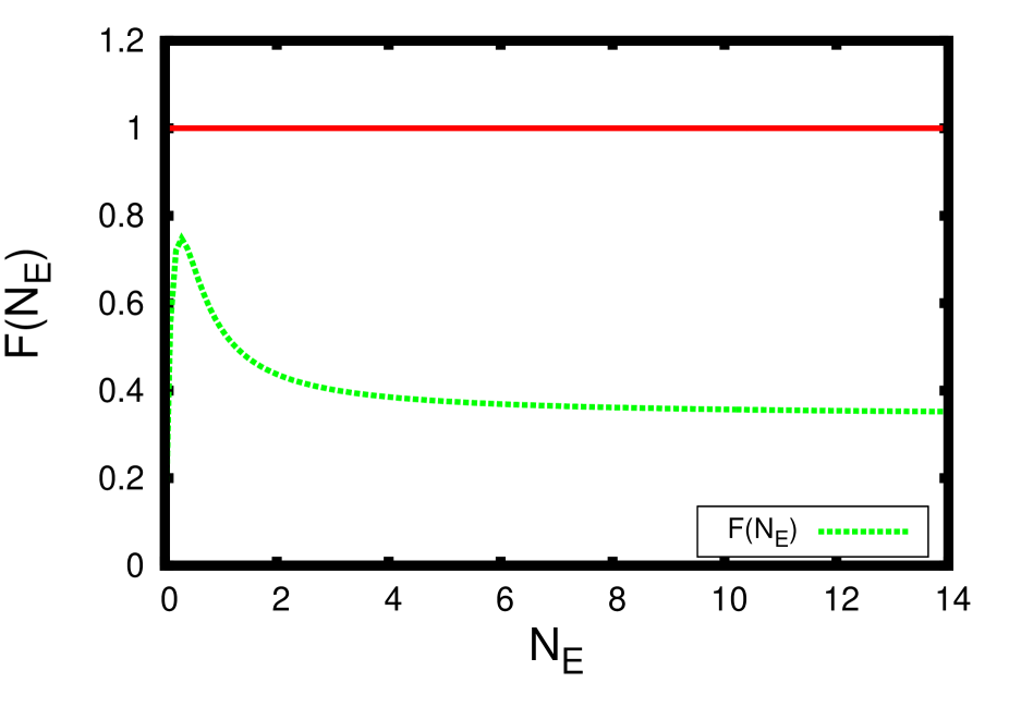
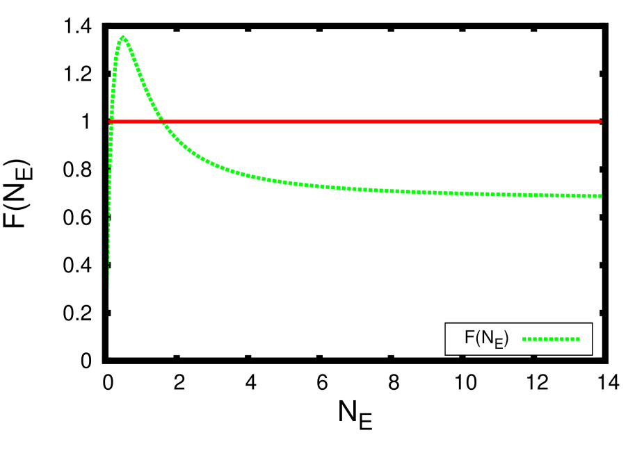
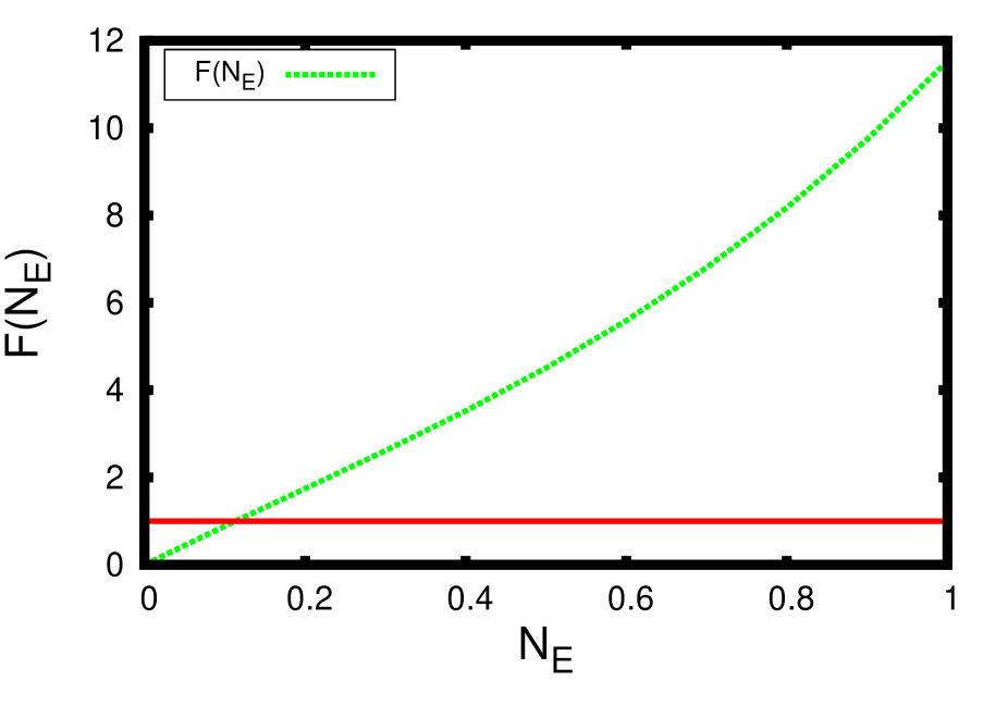
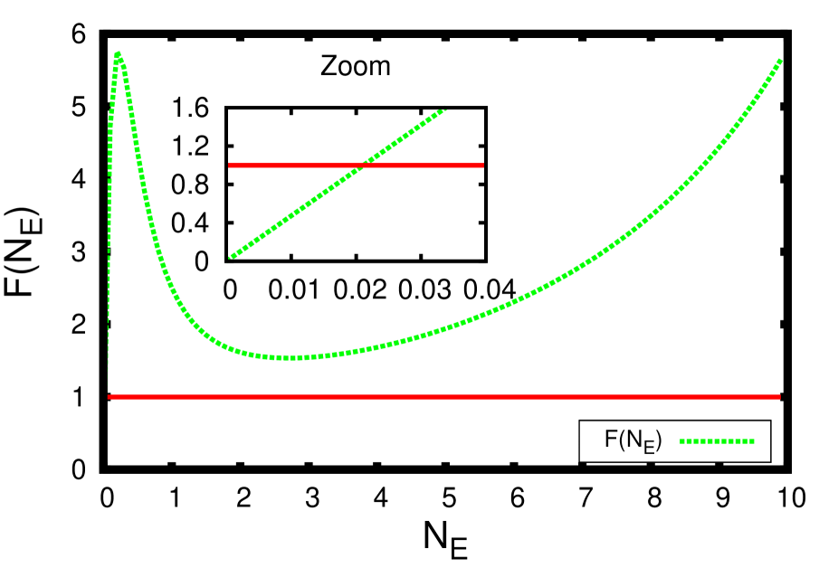
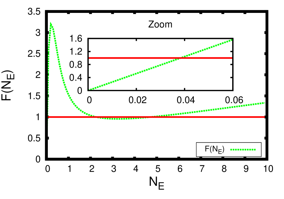
From a biological point of view, the previous analysis of the number of steady states shows the complexity of the set of stationary solutions in terms of the model parameters: the reset and threshold potentials, VRsubscript𝑉𝑅V_{R} and VFsubscript𝑉𝐹V_{F}, and the connectivity parameters, bEEsuperscriptsubscript𝑏𝐸𝐸b_{E}^{E}, bEIsuperscriptsubscript𝑏𝐸𝐼b_{E}^{I}, bIEsuperscriptsubscript𝑏𝐼𝐸b_{I}^{E} and bIIsuperscriptsubscript𝑏𝐼𝐼b_{I}^{I}, which describe the strengths of the synapses between excitatory and inhibitory neurons. For example, in function of the connectivity parameter bEEsuperscriptsubscript𝑏𝐸𝐸b_{E}^{E}, considering the rest of parameters fixed, we observe that if it is small (there are weak connections between excitatory neurons) there is a unique steady state. Whereas, if it is large (strong connections between excitatory neurons) there are no steady states. For intermediate values of bEEsuperscriptsubscript𝑏𝐸𝐸b_{E}^{E} different situations can occur: one, two or three steady states. In Section 5 we illustrate this complexity with numerical experiments (see Figs. 6, 7, 8, 9).

4.2 Long time behaviour

In [5] it was proved exponential convergence to the steady state for the linear case. Later, these results were extended in [8] to the nonlinear case, for a purely excitatory or inhibitory network with small connectivity parameters. In both papers the main tools used were the relative entropy and Poincaré inequalities. These techniques can be adapted for a coupled excitatory-inhibitory network, where the diffusion terms are considered constant, aαsubscript𝑎𝛼a_{\alpha}, where α=E,I𝛼𝐸𝐼\alpha=E,I. This is the goal of this subsection.

In Theorem 4.1 it was proved that for small connectivity parameters and constant diffusion terms there is only one stationary solution of the system (2.8)-(2.12), (ρE,ρI,NE,NI)superscriptsubscript𝜌𝐸superscriptsubscript𝜌𝐼superscriptsubscript𝑁𝐸superscriptsubscript𝑁𝐼\left(\rho_{E}^{\infty},\rho_{I}^{\infty},N_{E}^{\infty},N_{I}^{\infty}\right). Therefore, for any smooth convex function G:+:𝐺superscriptG:\mathbb{R}^{+}\to\mathbb{R}, we can define the relative entropy for α=E,I𝛼𝐸𝐼\alpha=E,I as

VFρα(v)G(ρα(v,t)ρα(v))𝑑v.superscriptsubscriptsubscript𝑉𝐹superscriptsubscript𝜌𝛼𝑣𝐺subscript𝜌𝛼𝑣𝑡superscriptsubscript𝜌𝛼𝑣differential-d𝑣\int_{-\infty}^{V_{F}}\rho_{\alpha}^{\infty}(v)G\left(\frac{\rho_{\alpha}(v,t)}{\rho_{\alpha}^{\infty}(v)}\right)\,dv.

Following similar computations to those developed in [5, 7, 8] for fast-decaying solutions to system (2.8)-(2.12), i.e. weak solutions for which the weak formulation holds for all test functions growing algebraically in v𝑣v, it can be obtained, for α=E,I𝛼𝐸𝐼\alpha=E,I:

ddtVFρα(v)G(ρα(v,t)ρα(v))𝑑v=aαVFρα(v)G′′(ρα(v,t)ρα(v))(vρα(v,t)ρα(v))2𝑑v𝑑𝑑𝑡superscriptsubscriptsubscript𝑉𝐹superscriptsubscript𝜌𝛼𝑣𝐺subscript𝜌𝛼𝑣𝑡superscriptsubscript𝜌𝛼𝑣differential-d𝑣subscript𝑎𝛼superscriptsubscriptsubscript𝑉𝐹superscriptsubscript𝜌𝛼𝑣superscript𝐺′′subscript𝜌𝛼𝑣𝑡superscriptsubscript𝜌𝛼𝑣superscript𝑣subscript𝜌𝛼𝑣𝑡superscriptsubscript𝜌𝛼𝑣2differential-d𝑣\displaystyle\frac{d}{dt}\int_{-\infty}^{V_{F}}\rho_{\alpha}^{\infty}(v)G\left(\frac{\rho_{\alpha}(v,t)}{\rho_{\alpha}^{\infty}(v)}\right)\,dv=-a_{\alpha}\int_{-\infty}^{V_{F}}\rho_{\alpha}^{\infty}(v)G^{\prime\prime}\left(\frac{\rho_{\alpha}(v,t)}{\rho_{\alpha}^{\infty}(v)}\right)\left(\frac{\partial}{\partial v}\frac{\rho_{\alpha}(v,t)}{\rho_{\alpha}^{\infty}(v)}\right)^{2}\ dv
Nα[G(Nα(t)Nα)G(ρα(VR,t)ρα(VR))(Nα(t)Nαρα(VR,t)ρα(VR))G(ρα(VR,t)ρα(VR))]superscriptsubscript𝑁𝛼delimited-[]𝐺subscript𝑁𝛼𝑡superscriptsubscript𝑁𝛼𝐺subscript𝜌𝛼subscript𝑉𝑅𝑡superscriptsubscript𝜌𝛼subscript𝑉𝑅subscript𝑁𝛼𝑡superscriptsubscript𝑁𝛼subscript𝜌𝛼subscript𝑉𝑅𝑡superscriptsubscript𝜌𝛼subscript𝑉𝑅superscript𝐺subscript𝜌𝛼subscript𝑉𝑅𝑡superscriptsubscript𝜌𝛼subscript𝑉𝑅\displaystyle-N_{\alpha}^{\infty}\left[G\left(\frac{N_{\alpha}(t)}{N_{\alpha}^{\infty}}\right)-G\left(\frac{\rho_{\alpha}(V_{R},t)}{\rho_{\alpha}^{\infty}(V_{R})}\right)-\left(\frac{N_{\alpha}(t)}{N_{\alpha}^{\infty}}-\frac{\rho_{\alpha}(V_{R},t)}{\rho_{\alpha}^{\infty}(V_{R})}\right)G^{\prime}\left(\frac{\rho_{\alpha}(V_{R},t)}{\rho_{\alpha}^{\infty}(V_{R})}\right)\right]
+(bEαN¯E(t)bIαN¯I(t))VFρα(t)v[G(ρα(v,t)ρα(v))(ρα(v,t)ρα(v))G(ρα(v,t)ρα(v))],superscriptsubscript𝑏𝐸𝛼subscript¯𝑁𝐸𝑡superscriptsubscript𝑏𝐼𝛼subscript¯𝑁𝐼𝑡superscriptsubscriptsubscript𝑉𝐹superscriptsubscript𝜌𝛼𝑡𝑣delimited-[]𝐺subscript𝜌𝛼𝑣𝑡superscriptsubscript𝜌𝛼𝑣subscript𝜌𝛼𝑣𝑡superscriptsubscript𝜌𝛼𝑣superscript𝐺subscript𝜌𝛼𝑣𝑡superscriptsubscript𝜌𝛼𝑣\displaystyle+\left(b_{E}^{\alpha}\bar{N}_{E}(t)-b_{I}^{\alpha}\bar{N}_{I}(t)\right)\int_{-\infty}^{V_{F}}\frac{\partial\rho_{\alpha}^{\infty}(t)}{\partial v}\left[G\left(\frac{\rho_{\alpha}(v,t)}{\rho_{\alpha}^{\infty}(v)}\right)-\left(\frac{\rho_{\alpha}(v,t)}{\rho_{\alpha}^{\infty}(v)}\right)G^{\prime}\left(\frac{\rho_{\alpha}(v,t)}{\rho_{\alpha}^{\infty}(v)}\right)\right], (4.16)

where N¯α(t)=Nα(t)Nαsubscript¯𝑁𝛼𝑡subscript𝑁𝛼𝑡superscriptsubscript𝑁𝛼\bar{N}_{\alpha}(t)=N_{\alpha}(t)-N_{\alpha}^{\infty}. Therefore, the entropy production of the relative entropy (its time derivative) for the excitatory (resp. inhibitory) population depends on the firing rate of the inhibitory (resp. excitatory) population. In other words, both entropy productions are linked by means of the firing rates. However, for the quadratic entropy, G(x)=(x1)2𝐺𝑥superscript𝑥12G(x)=\left(x-1\right)^{2}, a control on the sum of them,

E[t]:=VF[ρE(v)(ρE(v,t)ρE(v)1)2+ρI(v)(ρI(v,t)ρI(v)1)2]𝑑v,assign𝐸delimited-[]𝑡superscriptsubscriptsubscript𝑉𝐹delimited-[]superscriptsubscript𝜌𝐸𝑣superscriptsubscript𝜌𝐸𝑣𝑡superscriptsubscript𝜌𝐸𝑣12superscriptsubscript𝜌𝐼𝑣superscriptsubscript𝜌𝐼𝑣𝑡superscriptsubscript𝜌𝐼𝑣12differential-d𝑣E[t]:=\int_{-\infty}^{V_{F}}\left[\rho_{E}^{\infty}(v)\left(\frac{\rho_{E}(v,t)}{\rho_{E}^{\infty}(v)}-1\right)^{2}+\rho_{I}^{\infty}(v)\left(\frac{\rho_{I}(v,t)}{\rho_{I}^{\infty}(v)}-1\right)^{2}\right]\,dv, (4.17)

can be obtained for small connectivity parameters, proving an analogous result as in [8][Theorem 2.1].

Theorem 4.3

Assume aαsubscript𝑎𝛼a_{\alpha} constant for α=E,I𝛼𝐸𝐼\alpha=E,I, the connectivity parameters bEEsuperscriptsubscript𝑏𝐸𝐸b_{E}^{E}, bEIsuperscriptsubscript𝑏𝐸𝐼b_{E}^{I}, bIEsuperscriptsubscript𝑏𝐼𝐸b_{I}^{E} and bIIsuperscriptsubscript𝑏𝐼𝐼b_{I}^{I} small enough and initial data (ρE0,ρI0)superscriptsubscript𝜌𝐸0superscriptsubscript𝜌𝐼0(\rho_{E}^{0},\rho_{I}^{0}) such that

E[0]<12max(bEE+bIE,bEI+bII).𝐸delimited-[]012superscriptsubscript𝑏𝐸𝐸superscriptsubscript𝑏𝐼𝐸superscriptsubscript𝑏𝐸𝐼superscriptsubscript𝑏𝐼𝐼E[0]<\frac{1}{2\max\left(b_{E}^{E}+b_{I}^{E},b_{E}^{I}+b_{I}^{I}\right)}. (4.18)

Then, for fast decaying solutions to (2.8)-(2.12) there is a constant μ>0𝜇0\mu>0 such that, for all t0𝑡0t\geq 0,

E[t]eμtE[0].𝐸delimited-[]𝑡superscript𝑒𝜇𝑡𝐸delimited-[]0E[t]\leq e^{-\mu t}\,E[0].

Consequently, for α=E,I𝛼𝐸𝐼\alpha=E,I

VFρα(ρα(v,t)ρα(v)1)2𝑑veμtE[0].superscriptsubscriptsubscript𝑉𝐹superscriptsubscript𝜌𝛼superscriptsubscript𝜌𝛼𝑣𝑡superscriptsubscript𝜌𝛼𝑣12differential-d𝑣superscript𝑒𝜇𝑡𝐸delimited-[]0\int_{-\infty}^{V_{F}}\rho_{\alpha}^{\infty}\left(\frac{\rho_{\alpha}(v,t)}{\rho_{\alpha}^{\infty}(v)}-1\right)^{2}\,dv\leq e^{-\mu t}\,E[0].

Proof. The proof follows analogous steps as in [8][Theorem 2.1], with the main difficulty that, in this case, the entropy productions for excitatory and inhibitory populations are linked. This is the reason why the total relative entropy, given by the functional (4.17), has to be considered. Thus, the entropy production is the sum of the entropy productions of each population. In this way, the terms of N¯αsubscript¯𝑁𝛼\bar{N}_{\alpha} can be gathered and bound properly, as it is shown below.

Using (4.16) with G(x)=(x1)2𝐺𝑥superscript𝑥12G(x)=(x-1)^{2} for each term of the entropy (4.17), its time derivative can be written as

ddtE[t]𝑑𝑑𝑡𝐸delimited-[]𝑡\displaystyle\frac{d}{dt}E[t] =\displaystyle= 2aEVFρE(v)(vρE(v,t)ρE(v))2𝑑v2aIVFρI(v)(vρI(v,t)ρI(v))2𝑑v2subscript𝑎𝐸superscriptsubscriptsubscript𝑉𝐹superscriptsubscript𝜌𝐸𝑣superscript𝑣subscript𝜌𝐸𝑣𝑡superscriptsubscript𝜌𝐸𝑣2differential-d𝑣2subscript𝑎𝐼superscriptsubscriptsubscript𝑉𝐹superscriptsubscript𝜌𝐼𝑣superscript𝑣subscript𝜌𝐼𝑣𝑡superscriptsubscript𝜌𝐼𝑣2differential-d𝑣\displaystyle 2a_{E}\int_{-\infty}^{V_{F}}\rho_{E}^{\infty}(v)\left(\frac{\partial}{\partial v}\frac{\rho_{E}(v,t)}{\rho_{E}^{\infty}(v)}\right)^{2}\ dv-2a_{I}\int_{-\infty}^{V_{F}}\rho_{I}^{\infty}(v)\left(\frac{\partial}{\partial v}\frac{\rho_{I}(v,t)}{\rho_{I}^{\infty}(v)}\right)^{2}\ dv
\displaystyle- NE(NE(t)NEρE(VR,t)ρE(VR))2NI(NI(t)NIρI(VR,t)ρI(VR))2superscriptsubscript𝑁𝐸superscriptsubscript𝑁𝐸𝑡superscriptsubscript𝑁𝐸subscript𝜌𝐸subscript𝑉𝑅𝑡superscriptsubscript𝜌𝐸subscript𝑉𝑅2superscriptsubscript𝑁𝐼superscriptsubscript𝑁𝐼𝑡superscriptsubscript𝑁𝐼subscript𝜌𝐼subscript𝑉𝑅𝑡superscriptsubscript𝜌𝐼subscript𝑉𝑅2\displaystyle N_{E}^{\infty}\left(\frac{N_{E}(t)}{N_{E}^{\infty}}-\frac{\rho_{E}(V_{R},t)}{\rho_{E}^{\infty}(V_{R})}\right)^{2}-N_{I}^{\infty}\left(\frac{N_{I}(t)}{N_{I}^{\infty}}-\frac{\rho_{I}(V_{R},t)}{\rho_{I}^{\infty}(V_{R})}\right)^{2}
+\displaystyle+ 2(bEEN¯E(t)bIEN¯I(t))VFρE(v)[vρE(v,t)ρE(v)(ρE(v,t)ρE(v)1)+vρE(v,t)ρE(v)]𝑑v2superscriptsubscript𝑏𝐸𝐸subscript¯𝑁𝐸𝑡superscriptsubscript𝑏𝐼𝐸subscript¯𝑁𝐼𝑡superscriptsubscriptsubscript𝑉𝐹superscriptsubscript𝜌𝐸𝑣delimited-[]𝑣subscript𝜌𝐸𝑣𝑡superscriptsubscript𝜌𝐸𝑣subscript𝜌𝐸𝑣𝑡superscriptsubscript𝜌𝐸𝑣1𝑣subscript𝜌𝐸𝑣𝑡superscriptsubscript𝜌𝐸𝑣differential-d𝑣\displaystyle 2\left(b_{E}^{E}\bar{N}_{E}(t)-b_{I}^{E}\bar{N}_{I}(t)\right)\int_{-\infty}^{V_{F}}\rho_{E}^{\infty}(v)\left[\frac{\partial}{\partial v}\frac{\rho_{E}(v,t)}{\rho_{E}^{\infty}(v)}\left(\frac{\rho_{E}(v,t)}{\rho_{E}^{\infty}(v)}-1\right)+\frac{\partial}{\partial v}\frac{\rho_{E}(v,t)}{\rho_{E}^{\infty}(v)}\right]\ dv
+\displaystyle+ 2(bEIN¯E(t)bIIN¯I(t))VFρI(v)[vρI(v,t)ρI(v)(ρI(v,t)ρI(v)1)+vρI(v,t)ρI(v)]𝑑v,2superscriptsubscript𝑏𝐸𝐼subscript¯𝑁𝐸𝑡superscriptsubscript𝑏𝐼𝐼subscript¯𝑁𝐼𝑡superscriptsubscriptsubscript𝑉𝐹superscriptsubscript𝜌𝐼𝑣delimited-[]𝑣subscript𝜌𝐼𝑣𝑡superscriptsubscript𝜌𝐼𝑣subscript𝜌𝐼𝑣𝑡superscriptsubscript𝜌𝐼𝑣1𝑣subscript𝜌𝐼𝑣𝑡superscriptsubscript𝜌𝐼𝑣differential-d𝑣\displaystyle 2\left(b_{E}^{I}\bar{N}_{E}(t)-b_{I}^{I}\bar{N}_{I}(t)\right)\int_{-\infty}^{V_{F}}\rho_{I}^{\infty}(v)\left[\frac{\partial}{\partial v}\frac{\rho_{I}(v,t)}{\rho_{I}^{\infty}(v)}\left(\frac{\rho_{I}(v,t)}{\rho_{I}^{\infty}(v)}-1\right)+\frac{\partial}{\partial v}\frac{\rho_{I}(v,t)}{\rho_{I}^{\infty}(v)}\right]\ dv,

where the last two terms were obtained using that G(x)xG(x)=1x2𝐺𝑥𝑥superscript𝐺𝑥1superscript𝑥2G(x)-xG^{\prime}(x)=1-x^{2}, integrating by parts and taking into account the boundary conditions (2.9).

Considering the inequality (a+b)2ϵ(a22b2)superscript𝑎𝑏2italic-ϵsuperscript𝑎22superscript𝑏2(a+b)^{2}\geq\epsilon\left(a^{2}-2b^{2}\right), for a,b𝑎𝑏a,\,b\in\mathbb{R} and 0<ϵ<1/20italic-ϵ120<\epsilon<1/2, the Sobolev injection of L(I)superscript𝐿𝐼L^{\infty}(I) in H1(I)superscript𝐻1𝐼H^{1}(I) for a small neighborhood I𝐼I of VRsubscript𝑉𝑅V_{R}, where ραsuperscriptsubscript𝜌𝛼\rho_{\alpha}^{\infty} is bounded from below and the Poincaré inequality (see [5][Appendix] and [8] for details), the third and fourth terms in (4.2) satisfy:

Nα(Nα(t)Nαρα(VR,t)ρα(VR))2C0α(Nα(t)Nα1)2+aα2VFρα(v)(vρα(v,t)ρα(v,t))2𝑑v,superscriptsubscript𝑁𝛼superscriptsubscript𝑁𝛼𝑡superscriptsubscript𝑁𝛼subscript𝜌𝛼subscript𝑉𝑅𝑡superscriptsubscript𝜌𝛼subscript𝑉𝑅2superscriptsubscript𝐶0𝛼superscriptsubscript𝑁𝛼𝑡superscriptsubscript𝑁𝛼12subscript𝑎𝛼2superscriptsubscriptsubscript𝑉𝐹superscriptsubscript𝜌𝛼𝑣superscript𝑣subscript𝜌𝛼𝑣𝑡superscriptsubscript𝜌𝛼𝑣𝑡2differential-d𝑣\displaystyle-N_{\alpha}^{\infty}\left(\frac{N_{\alpha}(t)}{N_{\alpha}^{\infty}}-\frac{\rho_{\alpha}(V_{R},t)}{\rho_{\alpha}^{\infty}(V_{R})}\right)^{2}\leq-C_{0}^{\alpha}\left(\frac{N_{\alpha}(t)}{N_{\alpha}^{\infty}}-1\right)^{2}+\frac{a_{\alpha}}{2}\int_{-\infty}^{V_{F}}\rho_{\alpha}^{\infty}(v)\left(\frac{\partial}{\partial v}\frac{\rho_{\alpha}(v,t)}{\rho_{\alpha}^{\infty}}(v,t)\right)^{2}dv,

for some positive constant C0αsuperscriptsubscript𝐶0𝛼C_{0}^{\alpha}.

The estimate of the last two terms of (4.2) is quite more involved. First, each term is split into four addends, so that

2(bEαN¯E(t)bIαN¯I(t))VFρα(v)2superscriptsubscript𝑏𝐸𝛼subscript¯𝑁𝐸𝑡superscriptsubscript𝑏𝐼𝛼subscript¯𝑁𝐼𝑡superscriptsubscriptsubscript𝑉𝐹superscriptsubscript𝜌𝛼𝑣\displaystyle 2\left(b_{E}^{\alpha}\bar{N}_{E}(t)-b_{I}^{\alpha}\bar{N}_{I}(t)\right)\int_{-\infty}^{V_{F}}\rho_{\alpha}^{\infty}(v) [vρα(v,t)ρα(v)(ρα(v,t)ρα(v)1)+vρα(v,t)ρα(v)]dvdelimited-[]𝑣subscript𝜌𝛼𝑣𝑡superscriptsubscript𝜌𝛼𝑣subscript𝜌𝛼𝑣𝑡superscriptsubscript𝜌𝛼𝑣1𝑣subscript𝜌𝛼𝑣𝑡superscriptsubscript𝜌𝛼𝑣𝑑𝑣\displaystyle\!\!\!\!\!\!\!\!\!\!\!\!\!\!\left[\frac{\partial}{\partial v}\frac{\rho_{\alpha}(v,t)}{\rho_{\alpha}^{\infty}(v)}\left(\frac{\rho_{\alpha}(v,t)}{\rho_{\alpha}^{\infty}(v)}-1\right)+\frac{\partial}{\partial v}\frac{\rho_{\alpha}(v,t)}{\rho_{\alpha}^{\infty}(v)}\right]\ dv
=\displaystyle= 2bEαN¯E(t)VFρα(v)vρα(v,t)ρα(v)(ρα(v,t)ρα(v)1)𝑑v2superscriptsubscript𝑏𝐸𝛼subscript¯𝑁𝐸𝑡superscriptsubscriptsubscript𝑉𝐹superscriptsubscript𝜌𝛼𝑣𝑣subscript𝜌𝛼𝑣𝑡superscriptsubscript𝜌𝛼𝑣subscript𝜌𝛼𝑣𝑡superscriptsubscript𝜌𝛼𝑣1differential-d𝑣\displaystyle 2b_{E}^{\alpha}\bar{N}_{E}(t)\int_{-\infty}^{V_{F}}\rho_{\alpha}^{\infty}(v)\frac{\partial}{\partial v}\frac{\rho_{\alpha}(v,t)}{\rho_{\alpha}^{\infty}(v)}\left(\frac{\rho_{\alpha}(v,t)}{\rho_{\alpha}^{\infty}(v)}-1\right)\ dv
+2bEαN¯E(t)VFρα(v)vρα(v,t)ρα(v)𝑑v2superscriptsubscript𝑏𝐸𝛼subscript¯𝑁𝐸𝑡superscriptsubscriptsubscript𝑉𝐹superscriptsubscript𝜌𝛼𝑣𝑣subscript𝜌𝛼𝑣𝑡superscriptsubscript𝜌𝛼𝑣differential-d𝑣\displaystyle+2b_{E}^{\alpha}\bar{N}_{E}(t)\int_{-\infty}^{V_{F}}\rho_{\alpha}^{\infty}(v)\frac{\partial}{\partial v}\frac{\rho_{\alpha}(v,t)}{\rho_{\alpha}^{\infty}(v)}\ dv
2bIαN¯I(t)VFρα(v)vρα(v,t)ρα(v)(ρα(v,t)ρα(v)1)𝑑v2superscriptsubscript𝑏𝐼𝛼subscript¯𝑁𝐼𝑡superscriptsubscriptsubscript𝑉𝐹superscriptsubscript𝜌𝛼𝑣𝑣subscript𝜌𝛼𝑣𝑡superscriptsubscript𝜌𝛼𝑣subscript𝜌𝛼𝑣𝑡superscriptsubscript𝜌𝛼𝑣1differential-d𝑣\displaystyle-2b_{I}^{\alpha}\bar{N}_{I}(t)\int_{-\infty}^{V_{F}}\rho_{\alpha}^{\infty}(v)\frac{\partial}{\partial v}\frac{\rho_{\alpha}(v,t)}{\rho_{\alpha}^{\infty}(v)}\left(\frac{\rho_{\alpha}(v,t)}{\rho_{\alpha}^{\infty}(v)}-1\right)\ dv
2bIαN¯I(t)VFρα(v)vρα(v,t)ρα(v)𝑑v.2superscriptsubscript𝑏𝐼𝛼subscript¯𝑁𝐼𝑡superscriptsubscriptsubscript𝑉𝐹superscriptsubscript𝜌𝛼𝑣𝑣subscript𝜌𝛼𝑣𝑡superscriptsubscript𝜌𝛼𝑣differential-d𝑣\displaystyle-2b_{I}^{\alpha}\bar{N}_{I}(t)\int_{-\infty}^{V_{F}}\rho_{\alpha}^{\infty}(v)\frac{\partial}{\partial v}\frac{\rho_{\alpha}(v,t)}{\rho_{\alpha}^{\infty}(v)}\ dv.

Then, Cauchy-Schwarz’s and Young’s inequalities provide

2bEα2superscriptsubscript𝑏𝐸𝛼\displaystyle 2b_{E}^{\alpha} |N¯E(t)|VFρα(v)|vρα(v,t)ρα(v)(ρα(v,t)ρα(v)1)|𝑑vsubscript¯𝑁𝐸𝑡superscriptsubscriptsubscript𝑉𝐹superscriptsubscript𝜌𝛼𝑣𝑣subscript𝜌𝛼𝑣𝑡superscriptsubscript𝜌𝛼𝑣subscript𝜌𝛼𝑣𝑡superscriptsubscript𝜌𝛼𝑣1differential-d𝑣\displaystyle\!\!\!\!\!\!\!\!\!\!\!\!\!\!|\bar{N}_{E}(t)|\int_{-\infty}^{V_{F}}\rho_{\alpha}^{\infty}(v)\left|\frac{\partial}{\partial v}\frac{\rho_{\alpha}(v,t)}{\rho_{\alpha}^{\infty}(v)}\left(\frac{\rho_{\alpha}(v,t)}{\rho_{\alpha}^{\infty}(v)}-1\right)\right|\,dv
\displaystyle\leq bEαaE(NE)2(NE(t)NE1)2+aEbEαVFρα(v)(vρα(v,t)ρα(v))2𝑑vVFρα(v)(ρα(v,t)ρα(v)1)2𝑑vsuperscriptsubscript𝑏𝐸𝛼subscript𝑎𝐸superscriptsuperscriptsubscript𝑁𝐸2superscriptsubscript𝑁𝐸𝑡superscriptsubscript𝑁𝐸12subscript𝑎𝐸superscriptsubscript𝑏𝐸𝛼superscriptsubscriptsubscript𝑉𝐹superscriptsubscript𝜌𝛼𝑣superscript𝑣subscript𝜌𝛼𝑣𝑡superscriptsubscript𝜌𝛼𝑣2differential-d𝑣superscriptsubscriptsubscript𝑉𝐹superscriptsubscript𝜌𝛼𝑣superscriptsubscript𝜌𝛼𝑣𝑡superscriptsubscript𝜌𝛼𝑣12differential-d𝑣\displaystyle\frac{b_{E}^{\alpha}}{a_{E}}{(N_{E}^{\infty})}^{2}\left(\frac{N_{E}(t)}{N_{E}^{\infty}}-1\right)^{2}+a_{E}b_{E}^{\alpha}\int_{-\infty}^{V_{F}}\rho_{\alpha}^{\infty}(v)\left(\frac{\partial}{\partial v}\frac{\rho_{\alpha}(v,t)}{\rho_{\alpha}^{\infty}(v)}\right)^{2}\,dv\int_{-\infty}^{V_{F}}\rho_{\alpha}^{\infty}(v)\left(\frac{\rho_{\alpha}(v,t)}{\rho_{\alpha}^{\infty}(v)}-1\right)^{2}\,dv

and

2bEα|N¯E(t)|VFρα(v)|vρα(v,t)ρα(v)|𝑑v4(bEα)2aENE2(NE(t)NE1)2+aE4VFρα(v)(vρα(v,t)ρα(v))2𝑑v.2superscriptsubscript𝑏𝐸𝛼subscript¯𝑁𝐸𝑡superscriptsubscriptsubscript𝑉𝐹superscriptsubscript𝜌𝛼𝑣𝑣subscript𝜌𝛼𝑣𝑡superscriptsubscript𝜌𝛼𝑣differential-d𝑣4superscriptsuperscriptsubscript𝑏𝐸𝛼2subscript𝑎𝐸superscriptsuperscriptsubscript𝑁𝐸2superscriptsubscript𝑁𝐸𝑡superscriptsubscript𝑁𝐸12subscript𝑎𝐸4superscriptsubscriptsubscript𝑉𝐹superscriptsubscript𝜌𝛼𝑣superscript𝑣subscript𝜌𝛼𝑣𝑡superscriptsubscript𝜌𝛼𝑣2differential-d𝑣\displaystyle 2b_{E}^{\alpha}|\bar{N}_{E}(t)|\int_{-\infty}^{V_{F}}\rho_{\alpha}^{\infty}(v)\left|\frac{\partial}{\partial v}\frac{\rho_{\alpha}(v,t)}{\rho_{\alpha}^{\infty}(v)}\right|\,dv\leq 4\frac{{(b_{E}^{\alpha})}^{2}}{a_{E}}{N_{E}^{\infty}}^{2}\left(\frac{N_{E}(t)}{N_{E}^{\infty}}-1\right)^{2}+\frac{a_{E}}{4}\int_{-\infty}^{V_{F}}\rho_{\alpha}^{\infty}(v)\left(\frac{\partial}{\partial v}\frac{\rho_{\alpha}(v,t)}{\rho_{\alpha}^{\infty}(v)}\right)^{2}\,dv.

Getting these bounds together

ddtE[t]𝑑𝑑𝑡𝐸delimited-[]𝑡\displaystyle\frac{d}{dt}E[t] \displaystyle\leq (bEEaE+bEIaI+4(bEE)2aE+4(bEI)2aIC0ENE2)(NE)2(NE(t)NE1)2superscriptsubscript𝑏𝐸𝐸subscript𝑎𝐸superscriptsubscript𝑏𝐸𝐼subscript𝑎𝐼4superscriptsuperscriptsubscript𝑏𝐸𝐸2subscript𝑎𝐸4superscriptsuperscriptsubscript𝑏𝐸𝐼2subscript𝑎𝐼superscriptsubscript𝐶0𝐸superscriptsuperscriptsubscript𝑁𝐸2superscriptsuperscriptsubscript𝑁𝐸2superscriptsubscript𝑁𝐸𝑡superscriptsubscript𝑁𝐸12\displaystyle\left(\frac{b_{E}^{E}}{a_{E}}+\frac{b_{E}^{I}}{a_{I}}+4\frac{{(b_{E}^{E})}^{2}}{a_{E}}+4\frac{{(b_{E}^{I})}^{2}}{a_{I}}-\frac{C_{0}^{E}}{{N_{E}^{\infty}}^{2}}\right){(N_{E}^{\infty})}^{2}\left(\frac{N_{E}(t)}{N_{E}^{\infty}}-1\right)^{2}
+(bIEaE+bIIaI+4(bIE)2aE+4(bII)2aIC0INI2)(NI)2(NI(t)NI1)2superscriptsubscript𝑏𝐼𝐸subscript𝑎𝐸superscriptsubscript𝑏𝐼𝐼subscript𝑎𝐼4superscriptsuperscriptsubscript𝑏𝐼𝐸2subscript𝑎𝐸4superscriptsuperscriptsubscript𝑏𝐼𝐼2subscript𝑎𝐼superscriptsubscript𝐶0𝐼superscriptsuperscriptsubscript𝑁𝐼2superscriptsuperscriptsubscript𝑁𝐼2superscriptsubscript𝑁𝐼𝑡superscriptsubscript𝑁𝐼12\displaystyle+\left(\frac{b_{I}^{E}}{a_{E}}+\frac{b_{I}^{I}}{a_{I}}+4\frac{{(b_{I}^{E})}^{2}}{a_{E}}+4\frac{{(b_{I}^{I})}^{2}}{a_{I}}-\frac{C_{0}^{I}}{{N_{I}^{\infty}}^{2}}\right){(N_{I}^{\infty})}^{2}\left(\frac{N_{I}(t)}{N_{I}^{\infty}}-1\right)^{2}
aEVFρE(v)(vρE(v,t)ρE(v,t))2𝑑v[1(bEE+bEI)VFρE(v)(ρE(v,t)ρE(v,t)1)2𝑑v]subscript𝑎𝐸superscriptsubscriptsubscript𝑉𝐹superscriptsubscript𝜌𝐸𝑣superscript𝑣subscript𝜌𝐸𝑣𝑡superscriptsubscript𝜌𝐸𝑣𝑡2differential-d𝑣delimited-[]1superscriptsubscript𝑏𝐸𝐸superscriptsubscript𝑏𝐸𝐼superscriptsubscriptsubscript𝑉𝐹superscriptsubscript𝜌𝐸𝑣superscriptsubscript𝜌𝐸𝑣𝑡superscriptsubscript𝜌𝐸𝑣𝑡12differential-d𝑣\displaystyle-a_{E}\int_{-\infty}^{V_{F}}\rho_{E}^{\infty}(v)\left(\frac{\partial}{\partial v}\frac{\rho_{E}(v,t)}{\rho_{E}^{\infty}}(v,t)\right)^{2}dv\left[1-(b_{E}^{E}+b_{E}^{I})\int_{-\infty}^{V_{F}}\rho_{E}^{\infty}(v)\left(\frac{\rho_{E}(v,t)}{\rho_{E}^{\infty}}(v,t)-1\right)^{2}dv\right]
aIVFρI(v)(vρI(v,t)ρI(v,t))2𝑑v[1(bIE+bII)VFρI(v)(ρI(v,t)ρI(v,t)1)2𝑑v].subscript𝑎𝐼superscriptsubscriptsubscript𝑉𝐹superscriptsubscript𝜌𝐼𝑣superscript𝑣subscript𝜌𝐼𝑣𝑡superscriptsubscript𝜌𝐼𝑣𝑡2differential-d𝑣delimited-[]1superscriptsubscript𝑏𝐼𝐸superscriptsubscript𝑏𝐼𝐼superscriptsubscriptsubscript𝑉𝐹superscriptsubscript𝜌𝐼𝑣superscriptsubscript𝜌𝐼𝑣𝑡superscriptsubscript𝜌𝐼𝑣𝑡12differential-d𝑣\displaystyle-a_{I}\int_{-\infty}^{V_{F}}\rho_{I}^{\infty}(v)\left(\frac{\partial}{\partial v}\frac{\rho_{I}(v,t)}{\rho_{I}^{\infty}}(v,t)\right)^{2}dv\left[1-(b_{I}^{E}+b_{I}^{I})\int_{-\infty}^{V_{F}}\rho_{I}^{\infty}(v)\left(\frac{\rho_{I}(v,t)}{\rho_{I}^{\infty}}(v,t)-1\right)^{2}dv\right].

In this way, for bkαsuperscriptsubscript𝑏𝑘𝛼b_{k}^{\alpha} small enough such that (bαEaE+bαIaI+4(bαE)2aE+(bαI)2aIC0α(Nα)2)<0,superscriptsubscript𝑏𝛼𝐸subscript𝑎𝐸superscriptsubscript𝑏𝛼𝐼subscript𝑎𝐼4superscriptsuperscriptsubscript𝑏𝛼𝐸2subscript𝑎𝐸superscriptsuperscriptsubscript𝑏𝛼𝐼2subscript𝑎𝐼superscriptsubscript𝐶0𝛼superscriptsuperscriptsubscript𝑁𝛼20\left(\frac{b_{\alpha}^{E}}{a_{E}}+\frac{b_{\alpha}^{I}}{a_{I}}+4\frac{{(b_{\alpha}^{E})}^{2}}{a_{E}}+\frac{{(b_{\alpha}^{I})}^{2}}{a_{I}}-\frac{C_{0}^{\alpha}}{{(N_{\alpha}^{\infty})}^{2}}\right)<0, the first and second terms of the right hand side of (4.2) are negative, thus

ddtE[t]𝑑𝑑𝑡𝐸delimited-[]𝑡\displaystyle\frac{d}{dt}E[t] \displaystyle\!\!\leq aEVFρE(v)(vρE(v,t)ρE(v,t))2𝑑v[1(bEE+bEI)VFρE(v)(ρE(v,t)ρE(v,t)1)2𝑑v]subscript𝑎𝐸superscriptsubscriptsubscript𝑉𝐹superscriptsubscript𝜌𝐸𝑣superscript𝑣subscript𝜌𝐸𝑣𝑡superscriptsubscript𝜌𝐸𝑣𝑡2differential-d𝑣delimited-[]1superscriptsubscript𝑏𝐸𝐸superscriptsubscript𝑏𝐸𝐼superscriptsubscriptsubscript𝑉𝐹superscriptsubscript𝜌𝐸𝑣superscriptsubscript𝜌𝐸𝑣𝑡superscriptsubscript𝜌𝐸𝑣𝑡12differential-d𝑣\displaystyle\!\!-a_{E}\int_{-\infty}^{V_{F}}\rho_{E}^{\infty}(v)\left(\frac{\partial}{\partial v}\frac{\rho_{E}(v,t)}{\rho_{E}^{\infty}}(v,t)\right)^{2}\!\!\!\!dv\left[1-(b_{E}^{E}+b_{E}^{I})\int_{-\infty}^{V_{F}}\rho_{E}^{\infty}(v)\left(\frac{\rho_{E}(v,t)}{\rho_{E}^{\infty}}(v,t)-1\right)^{2}\!\!\!\!dv\right] (4.21)
\displaystyle\!\!\!\!\!\!- aIVFρI(v)(vρI(v,t)ρI(v,t))2𝑑v[1(bIE+bII)VFρI(v)(ρI(v,t)ρI(v,t)1)2𝑑v].subscript𝑎𝐼superscriptsubscriptsubscript𝑉𝐹superscriptsubscript𝜌𝐼𝑣superscript𝑣subscript𝜌𝐼𝑣𝑡superscriptsubscript𝜌𝐼𝑣𝑡2differential-d𝑣delimited-[]1superscriptsubscript𝑏𝐼𝐸superscriptsubscript𝑏𝐼𝐼superscriptsubscriptsubscript𝑉𝐹superscriptsubscript𝜌𝐼𝑣superscriptsubscript𝜌𝐼𝑣𝑡superscriptsubscript𝜌𝐼𝑣𝑡12differential-d𝑣\displaystyle\!\!\!\!\!\!a_{I}\int_{-\infty}^{V_{F}}\rho_{I}^{\infty}(v)\left(\frac{\partial}{\partial v}\frac{\rho_{I}(v,t)}{\rho_{I}^{\infty}}(v,t)\right)^{2}\!\!\!\!dv\left[1-(b_{I}^{E}+b_{I}^{I})\int_{-\infty}^{V_{F}}\rho_{I}^{\infty}(v)\left(\frac{\rho_{I}(v,t)}{\rho_{I}^{\infty}}(v,t)-1\right)^{2}\!\!\!\!dv\right]\!\!.

Denoting C=max(bEE+bIE,bEI+bII)𝐶superscriptsubscript𝑏𝐸𝐸superscriptsubscript𝑏𝐼𝐸superscriptsubscript𝑏𝐸𝐼superscriptsubscript𝑏𝐼𝐼C=\max\left(b_{E}^{E}+b_{I}^{E},b_{E}^{I}+b_{I}^{I}\right), the entropy production can be bounded as follows

ddtE[t]VF[aEρE(v)(vρE(v,t)ρE(v,t))2+aIρI(v)(vρI(v,t)ρI(v,t))2]𝑑v(1CE[t]).𝑑𝑑𝑡𝐸delimited-[]𝑡superscriptsubscriptsubscript𝑉𝐹delimited-[]subscript𝑎𝐸superscriptsubscript𝜌𝐸𝑣superscript𝑣subscript𝜌𝐸𝑣𝑡superscriptsubscript𝜌𝐸𝑣𝑡2subscript𝑎𝐼superscriptsubscript𝜌𝐼𝑣superscript𝑣subscript𝜌𝐼𝑣𝑡superscriptsubscript𝜌𝐼𝑣𝑡2differential-d𝑣1𝐶𝐸delimited-[]𝑡\frac{d}{dt}E[t]\leq-\int_{-\infty}^{V_{F}}\left[a_{E}\rho_{E}^{\infty}(v)\left(\frac{\partial}{\partial v}\frac{\rho_{E}(v,t)}{\rho_{E}^{\infty}}(v,t)\right)^{2}+a_{I}\rho_{I}^{\infty}(v)\left(\frac{\partial}{\partial v}\frac{\rho_{I}(v,t)}{\rho_{I}^{\infty}}(v,t)\right)^{2}\right]dv\left(1-CE[t]\right). (4.22)

Now, using (4.18) and Gronwall’s inequality it can be proved that E[t]𝐸delimited-[]𝑡E[t] decreases for all times and E[t]<12C𝐸delimited-[]𝑡12𝐶E[t]<\frac{1}{2C}, for all t>0𝑡0t>0. Thus,

ddtE[t]aE2VFρE(v)(vρE(v,t)ρE(v,t))2𝑑vaI2VFρI(v)(vρI(v,t)ρI(v,t))2𝑑v.𝑑𝑑𝑡𝐸delimited-[]𝑡subscript𝑎𝐸2superscriptsubscriptsubscript𝑉𝐹superscriptsubscript𝜌𝐸𝑣superscript𝑣subscript𝜌𝐸𝑣𝑡superscriptsubscript𝜌𝐸𝑣𝑡2differential-d𝑣subscript𝑎𝐼2superscriptsubscriptsubscript𝑉𝐹superscriptsubscript𝜌𝐼𝑣superscript𝑣subscript𝜌𝐼𝑣𝑡superscriptsubscript𝜌𝐼𝑣𝑡2differential-d𝑣\frac{d}{dt}E[t]\leq-\frac{a_{E}}{2}\int_{-\infty}^{V_{F}}\rho_{E}^{\infty}(v)\left(\frac{\partial}{\partial v}\frac{\rho_{E}(v,t)}{\rho_{E}^{\infty}}(v,t)\right)^{2}dv-\frac{a_{I}}{2}\int_{-\infty}^{V_{F}}\rho_{I}^{\infty}(v)\left(\frac{\partial}{\partial v}\frac{\rho_{I}(v,t)}{\rho_{I}^{\infty}}(v,t)\right)^{2}dv.

Applying the Poincaré inequality on each term, there exist γ,γ>0𝛾superscript𝛾0\gamma,\,\gamma^{\prime}>0 such that

ddtE[t]aEγ2VFρE(v)(ρα(v,t)ρE(v)1)2𝑑vaIγ2VFρI(v)(ρα(v,t)ρI(v)1)2𝑑v.𝑑𝑑𝑡𝐸delimited-[]𝑡subscript𝑎𝐸𝛾2superscriptsubscriptsubscript𝑉𝐹superscriptsubscript𝜌𝐸𝑣superscriptsubscript𝜌𝛼𝑣𝑡superscriptsubscript𝜌𝐸𝑣12differential-d𝑣subscript𝑎𝐼superscript𝛾2superscriptsubscriptsubscript𝑉𝐹superscriptsubscript𝜌𝐼𝑣superscriptsubscript𝜌𝛼𝑣𝑡superscriptsubscript𝜌𝐼𝑣12differential-d𝑣\frac{d}{dt}E[t]\leq-\frac{a_{E}\gamma}{2}\int_{-\infty}^{V_{F}}\rho_{E}^{\infty}(v)\left(\frac{\rho_{\alpha}(v,t)}{\rho_{E}^{\infty}(v)}-1\right)^{2}\,dv-\frac{a_{I}\gamma^{\prime}}{2}\int_{-\infty}^{V_{F}}\rho_{I}^{\infty}(v)\left(\frac{\rho_{\alpha}(v,t)}{\rho_{I}^{\infty}(v)}-1\right)^{2}\,dv.

Considering now μ=min(aEγ2,aIγ2)𝜇subscript𝑎𝐸𝛾2subscript𝑎𝐼superscript𝛾2\mu=\min\left(\frac{a_{E}\gamma}{2},\frac{a_{I}\gamma^{\prime}}{2}\right) we obtain ddtE[t]μE[t]𝑑𝑑𝑡𝐸delimited-[]𝑡𝜇𝐸delimited-[]𝑡\frac{d}{dt}E[t]\leq-\mu E[t]. Finally, Gronwall’s inequality concludes the proof.       

5 Numerical results

The analytical results proved in previous sections are shown numerically in the present section. The numerical scheme considered for this purpose is based on a fifth order conservative finite difference WENO (Weighted Essentially Non-Oscillatory) scheme for the advection term, standard second order centered finite differences for the diffusion term and an explicit third order TVD (Total Variation Diminishing) Runge-Kutta scheme for the time evolution. To reduce the computation time, parallel computation techniques for a two cores code is developed. Thus, the time evolution for both equations of the system is calculated simultaneously. Each core handles one of the equations. MPI (Message Passing Interface) communication between the cores has been included in the code, since the system is coupled by the firing rates. Therefore, at the end of each Runge-Kutta step, each core needs to know the value of the firing rate of the other core.

For the simulations, an uniform mesh for v[Vleft,VF]𝑣subscript𝑉𝑙𝑒𝑓𝑡subscript𝑉𝐹v\in[-V_{left},V_{F}] is considered. The value of Vleftsubscript𝑉𝑙𝑒𝑓𝑡-V_{left} is chosen such that ρα(Vleft,t)0similar-tosubscript𝜌𝛼subscript𝑉𝑙𝑒𝑓𝑡𝑡0\rho_{\alpha}(-V_{left},t)\sim 0 (since ρα(,t)=0subscript𝜌𝛼𝑡0\rho_{\alpha}(-\infty,t)=0). The time step size is adapted dynamically during the simulations via a CFL (Courant-Friedrich-Levy) time step condition. Some parameter values are common to most simulations, VF=2subscript𝑉𝐹2V_{F}=2, VR=1subscript𝑉𝑅1V_{R}=1 and νE,ext=0subscript𝜈𝐸𝑒𝑥𝑡0\nu_{E,ext}=0 and the diffusion terms aα(NE,NI)subscript𝑎𝛼subscript𝑁𝐸subscript𝑁𝐼a_{\alpha}(N_{E},N_{I}) have been taken constant as aα=1subscript𝑎𝛼1a_{\alpha}=1. In the simulations where these values are different, the considered values are indicated in their figures and explanations. In most cases, the initial condition is

ρα0(v)=k2πe(vv0α)22σ0α2,subscriptsuperscript𝜌0𝛼𝑣𝑘2𝜋superscript𝑒superscript𝑣superscriptsubscript𝑣0𝛼22superscriptsuperscriptsubscript𝜎0𝛼2\rho^{0}_{\alpha}(v)=\frac{k}{\sqrt{2\pi}}e^{-\frac{(v-v_{0}^{\alpha})^{2}}{2{\sigma_{0}^{\alpha}}^{2}}}, (5.1)

where k𝑘k is a constant such that VleftVFρα0(v)𝑑v1superscriptsubscriptsubscript𝑉𝑙𝑒𝑓𝑡subscript𝑉𝐹subscriptsuperscript𝜌0𝛼𝑣differential-d𝑣1\displaystyle\int_{-V_{left}}^{V_{F}}\rho^{0}_{\alpha}(v)\ dv\approx 1 numerically. However, in order to analyze the stability of steady states, stationary profiles are taken as initial conditions

ρα0(v)=Nαaα(NE,NI)e(vV0α(NE,NI))22aα(NE,NI)max(v,VR)VFe(wV0α(NE,NI))22aα(NE,NI)𝑑w,α=E,I,formulae-sequencesuperscriptsubscript𝜌𝛼0𝑣subscript𝑁𝛼subscript𝑎𝛼subscript𝑁𝐸subscript𝑁𝐼superscript𝑒superscript𝑣superscriptsubscript𝑉0𝛼subscript𝑁𝐸subscript𝑁𝐼22subscript𝑎𝛼subscript𝑁𝐸subscript𝑁𝐼superscriptsubscript𝑣subscript𝑉𝑅subscript𝑉𝐹superscript𝑒superscript𝑤superscriptsubscript𝑉0𝛼subscript𝑁𝐸subscript𝑁𝐼22subscript𝑎𝛼subscript𝑁𝐸subscript𝑁𝐼differential-d𝑤𝛼𝐸𝐼\rho_{\alpha}^{0}(v)=\frac{N_{\alpha}}{a_{\alpha}(N_{E},N_{I})}e^{-\frac{(v-V_{0}^{\alpha}(N_{E},N_{I}))^{2}}{2a_{\alpha}(N_{E},N_{I})}}\int_{\max(v,V_{R})}^{V_{F}}e^{\frac{(w-V_{0}^{\alpha}(N_{E},N_{I}))^{2}}{2a_{\alpha}(N_{E},N_{I})}}\ dw,\quad\alpha=E,I, (5.2)

with V0α(NE,NI)=bEαNEbIαNI+(bEαbEE)νE,extsuperscriptsubscript𝑉0𝛼subscript𝑁𝐸subscript𝑁𝐼superscriptsubscript𝑏𝐸𝛼subscript𝑁𝐸superscriptsubscript𝑏𝐼𝛼subscript𝑁𝐼superscriptsubscript𝑏𝐸𝛼superscriptsubscript𝑏𝐸𝐸subscript𝜈𝐸𝑒𝑥𝑡V_{0}^{\alpha}(N_{E},N_{I})=b_{E}^{\alpha}N_{E}-b_{I}^{\alpha}N_{I}+(b_{E}^{\alpha}-b_{E}^{E})\nu_{E,ext} and where Nαsubscript𝑁𝛼N_{\alpha} is an approximated value of the stationary firing rate.

To get an idea about the number of steady states, the system (4.3) is solved numerically. For every NEsubscript𝑁𝐸N_{E} fixed, NI(NE)subscript𝑁𝐼subscript𝑁𝐸N_{I}(N_{E}) is calculated as the root of NI(NE)I2(NE,NI(NE))1=0subscript𝑁𝐼subscript𝑁𝐸subscript𝐼2subscript𝑁𝐸subscript𝑁𝐼subscript𝑁𝐸10N_{I}(N_{E})I_{2}(N_{E},N_{I}(N_{E}))-1=0 using the bisection method with tolerance 108superscript10810^{-8}, and then a numerical approximation of (NE)subscript𝑁𝐸\mathcal{F}(N_{E}) is developed by quadrature formulas to find the number of intersections with the function 1. Fig. 2 shows the graphics of NI2(NE)I(NE)superscriptsubscript𝑁𝐼2subscript𝑁𝐸𝐼subscript𝑁𝐸N_{I}^{2}(N_{E})I(N_{E}) (see (4.12)) and (NE)subscript𝑁𝐸\mathcal{F}(N_{E}) for parameter values for which the limit of (NE)subscript𝑁𝐸\mathcal{F}(N_{E}) is finite. The numerical approximation of the limits is in agreement with their analytical limits.

Blow-up. Numerical results for three situations in which the solutions are not global-in-time are described. In Fig. 3 we depict a blow-up situation produced by a big value of bEEsuperscriptsubscript𝑏𝐸𝐸b_{E}^{E}, where the initial datum is far from VFsubscript𝑉𝐹V_{F}. However, for a value of the connectivity parameter bEEsuperscriptsubscript𝑏𝐸𝐸b_{E}^{E} small, we show a blow-up situation originated by an initial condition quite concentrated around VFsubscript𝑉𝐹V_{F} in Fig. 4. In both cases we observe that an extremely fast increase of the firing rate of the excitatory population causes the blow-up of the system. Furthermore, we notice that the firing rate of the inhibitory population also starts to grow sharply. Nevertheless, the values it takes are quite small in comparison with those from the excitatory population.

For a purely inhibitory network the global existence of its solutions was proved in [9]. Therefore, one could think that high values of bIIsuperscriptsubscript𝑏𝐼𝐼b_{I}^{I} could prevent the blow-up of the excitatory-inhibitory system. However, Theorem 3.1 shows that this is not the case and Fig. 5 describes this situation; although the value of bIIsuperscriptsubscript𝑏𝐼𝐼b_{I}^{I} is big, a high value of bEEsuperscriptsubscript𝑏𝐸𝐸b_{E}^{E} causes the divergence of NE(t)subscript𝑁𝐸𝑡N_{E}(t) and the blow-up of the system.

Steady states. The proof of Theorem 4.1 provides a strategy to find numerically the stationary firing rates, which consists of finding the intersection points between the functions (NE)subscript𝑁𝐸\mathcal{F}(N_{E}) and constant 1 (see (4.13)). With this idea, we have plotted both functions for different parameter values.

The first case of Theorem 4.1 (there is an even number of steady states or there are no steady states) is shown in Fig. 6. In this situation, the relation between the parameters implies limNE(NE)<1subscriptsubscript𝑁𝐸subscript𝑁𝐸1\displaystyle\lim_{N_{E}\to\infty}\mathcal{F}(N_{E})<1. In the left plot, the pure connectivity parameters (bEEsuperscriptsubscript𝑏𝐸𝐸b_{E}^{E} and bIIsuperscriptsubscript𝑏𝐼𝐼b_{I}^{I}) are high in comparison with the connectivity parameters bEIsuperscriptsubscript𝑏𝐸𝐼b_{E}^{I} and bIEsuperscriptsubscript𝑏𝐼𝐸b_{I}^{E}, in such a way that there are no steady states. In the right plot, there are two steady states because the pure connectivity parameters are small, since in this case the maximum value of \mathcal{F} is bigger than one.

The second case of Theorem 4.1 (there is an odd number of steady states), which implies limNE(NE)>1subscriptsubscript𝑁𝐸subscript𝑁𝐸1\displaystyle\lim_{N_{E}\to\infty}\mathcal{F}(N_{E})>1, is depicted in Fig. 7. In the left plot, bEEsuperscriptsubscript𝑏𝐸𝐸b_{E}^{E} is small enough such that \mathcal{F} is an increasing function, and therefore there is a unique steady state. Also, in the center plot there is only one stationary solution, but in this case the values of connectivity parameters do not guarantee the monotonicity of \mathcal{F}. Finally, the right plot shows values of connectivity parameters for which there are three steady states.

To conclude the analysis of the number of steady states, in Fig. 8 it is depicted a comparison between an uncoupled excitatory-inhibitory network (bEI=bIE=0superscriptsubscript𝑏𝐸𝐼superscriptsubscript𝑏𝐼𝐸0b_{E}^{I}=b_{I}^{E}=0) and a coupled network with small bEIsuperscriptsubscript𝑏𝐸𝐼b_{E}^{I} and bIEsuperscriptsubscript𝑏𝐼𝐸b_{I}^{E}. In Fig. 8 (left) the number of steady states for the uncoupled system (bEI=bIE=0superscriptsubscript𝑏𝐸𝐼superscriptsubscript𝑏𝐼𝐸0b_{E}^{I}=b_{I}^{E}=0) is analyzed, while Fig. 8 (right) investigates the number of steady states when the parameters bEIsuperscriptsubscript𝑏𝐸𝐼b_{E}^{I} and bIEsuperscriptsubscript𝑏𝐼𝐸b_{I}^{E} are small (bEI=bIE=0.1superscriptsubscript𝑏𝐸𝐼superscriptsubscript𝑏𝐼𝐸0.1b_{E}^{I}=b_{I}^{E}=0.1). As expected, it can be observed that the number of steady states does not change if we choose small values for bEIsuperscriptsubscript𝑏𝐸𝐼b_{E}^{I} and bIEsuperscriptsubscript𝑏𝐼𝐸b_{I}^{E}. It depends only on the value of bEEsuperscriptsubscript𝑏𝐸𝐸b_{E}^{E} in the same way as described in [5]. For small values of bEEsuperscriptsubscript𝑏𝐸𝐸b_{E}^{E} there is a unique steady state. As bEEsuperscriptsubscript𝑏𝐸𝐸b_{E}^{E} increases, it appears another steady state, that merges with the first one and then disappears, apparently yielding a saddle node bifurcation. In Fig. 10 we show the time evolution of the firing rates, for the case described in Fig. 6 (right), with two steady states. We use as initial condition profiles like the one presented in (5.2). The numerical results show that the larger steady state is unstable, while the lower one seems to be stable. Therefore, numerical stability analysis indicates that the unique steady state is stable, while, when there are two steady states the highest seems to be unstable.

In this direction, another interesting bifurcation analysis that can be obtained in terms of the parameter bIEsuperscriptsubscript𝑏𝐼𝐸b_{I}^{E} is depicted in Fig. 9. For large values of bEIsuperscriptsubscript𝑏𝐸𝐼b_{E}^{I} there is a unique stable steady. Then, as it decreases it appears another steady state that bifurcates and gives rise to two equilibria. The largest disappears, and the lower one approaches the smallest steady state. Afterwards, both disappear, probably through a saddle node bifurcation. Numerical stability analysis determines that the lowest steady state is always stable, while the other ones are all unstable. The Fig. 7 (right) depicts three steady states. The stability analysis of this situation is more complicated than the previous one (the case of two stationary solutions). Fig. 11 shows the time evolution of the solutions for different initial data; the steady state with less firing rate seems to be stable, while the other two steady states are unstable.

In conclusion, in the present work we have extended the known results for purely excitatory or inhibitory networks [5] to excitatory-inhibitory coupled networks. We have proved that the presence of an inhibitory population in a coupled network does not avoid the blow-up phenomenon, as happens in a purely inhibitory network. Besides, we have analysed the number of steady states of the system, which is a more complicate issue than in the case of uncoupled systems. For small connectivity parameter values, we have shown that solutions converge exponentially fast to the unique steady state. Our analytical and numerical results contribute to support the NNLIF system as an appropriate model to describe well known neurophysiological phenomena, as for example synchronization/asynchronization of the network, since the blow-up in finite time might depict a synchronization of a part of the network, while the presence of a unique asymptotically stable stationary solution represents an asynchronization of the network. In addition, the abundance in the number of steady states, in terms of the connectivity parameter values, that can be observed for this simplified model, probably will help us to characterize situations of multi-stability for more complete NNLIF models and also other models including conductance variables as in [6]. In [7] it was shown that if a refractory period is included in the model, there are situations of multi-stability, with two stable and one unstable steady state. In [6] bi-stability phenomena were numerically described. Multi-stable networks are related, for instance, to the visual perception and the decision making [18, 1]. In these directions, some tasks which remain open for the NNLIF model are: The analytical study of the stability of the network when there is more than one steady state, the possible presence of periodic solutions and the existence of solutions for coupled networks, maybe following a similiar strategy as in [17]. A more extensive bifurcation analysis could probably contribute to find answers to these questions.

Acknowledgments. The authors acknowledge support from the project MTM2014-52056-P of Spanish Ministerio de Economía y Competitividad and the European Regional Development Fund (ERDF/FEDER).
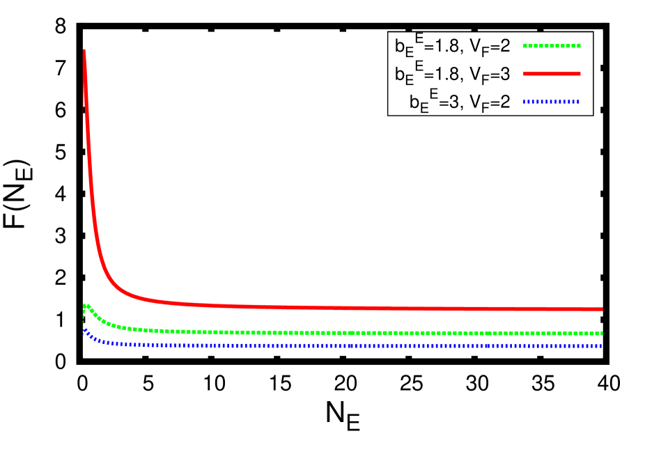
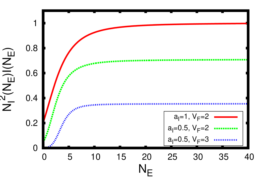
Refer to caption
Refer to caption
Figure 2: Study of the limits of (NE)subscript𝑁𝐸\mathcal{F}(N_{E}) and NI2(NE)I(NE)superscriptsubscript𝑁𝐼2subscript𝑁𝐸𝐼subscript𝑁𝐸N_{I}^{2}(N_{E})I(N_{E}) (see (4.12)) when it is finite.
Left figure: bIE=0.75superscriptsubscript𝑏𝐼𝐸0.75b_{I}^{E}=0.75, bEI=0.5superscriptsubscript𝑏𝐸𝐼0.5b_{E}^{I}=0.5, bII=0.25superscriptsubscript𝑏𝐼𝐼0.25b_{I}^{I}=0.25, aE=1subscript𝑎𝐸1a_{E}=1, aI=1subscript𝑎𝐼1a_{I}=1 for different values of bEEsuperscriptsubscript𝑏𝐸𝐸b_{E}^{E} and VFsubscript𝑉𝐹V_{F}.
Right figure: bEE=1.8superscriptsubscript𝑏𝐸𝐸1.8b_{E}^{E}=1.8, bIE=0.75superscriptsubscript𝑏𝐼𝐸0.75b_{I}^{E}=0.75, bEI=0.5superscriptsubscript𝑏𝐸𝐼0.5b_{E}^{I}=0.5, bII=0.25superscriptsubscript𝑏𝐼𝐼0.25b_{I}^{I}=0.25 aE=1subscript𝑎𝐸1a_{E}=1 for different values of aIsubscript𝑎𝐼a_{I} and VFsubscript𝑉𝐹V_{F}.
Refer to caption
Refer to caption
Refer to caption
Figure 3: Firing rates and probability densities for bEE=3superscriptsubscript𝑏𝐸𝐸3b_{E}^{E}=3, bIE=0.75superscriptsubscript𝑏𝐼𝐸0.75b_{I}^{E}=0.75, bEI=0.5superscriptsubscript𝑏𝐸𝐼0.5b_{E}^{I}=0.5, bII=0.25superscriptsubscript𝑏𝐼𝐼0.25b_{I}^{I}=0.25, in case of a normalized Maxwellian initial condition with mean 0 and variance 0.5 (see (5.1)). NEsubscript𝑁𝐸N_{E} blows-up because of the large value of bEEsuperscriptsubscript𝑏𝐸𝐸b_{E}^{E}.
Refer to caption
Refer to caption
Refer to caption
Figure 4: Firing rates and probability densities for bEE=0.5superscriptsubscript𝑏𝐸𝐸0.5b_{E}^{E}=0.5, bIE=0.25superscriptsubscript𝑏𝐼𝐸0.25b_{I}^{E}=0.25, bEI=0.25superscriptsubscript𝑏𝐸𝐼0.25b_{E}^{I}=0.25, bII=1superscriptsubscript𝑏𝐼𝐼1b_{I}^{I}=1, in case of a normalized concentrated Maxwellian initial condition with mean 1.83 and variance 0.003 (see (5.1)).The initial condition concentrated close to VFsubscript𝑉𝐹V_{F} provokes the blow-up of NEsubscript𝑁𝐸N_{E}.
Refer to caption
Refer to caption
Refer to caption
Figure 5: Firing rates and probability densities for bEE=3superscriptsubscript𝑏𝐸𝐸3b_{E}^{E}=3, bIE=0.75superscriptsubscript𝑏𝐼𝐸0.75b_{I}^{E}=0.75, bEI=0.5superscriptsubscript𝑏𝐸𝐼0.5b_{E}^{I}=0.5, bII=3superscriptsubscript𝑏𝐼𝐼3b_{I}^{I}=3, in case of a normalized Maxwellian initial condition with mean 0 and variance 0.5 (see (5.1)).The blow-up of NEsubscript𝑁𝐸N_{E} cannot be avoided by a large value of bIIsuperscriptsubscript𝑏𝐼𝐼b_{I}^{I}.
Refer to caption
Refer to caption
Figure 6: (NE)subscript𝑁𝐸\mathcal{F}(N_{E}) for different parameter values corresponding to the first case of Theorem 4.1: there are no steady states (left) or there is an even number of steady states (right).
Left figure: bEE=3superscriptsubscript𝑏𝐸𝐸3b_{E}^{E}=3, bIE=0.75superscriptsubscript𝑏𝐼𝐸0.75b_{I}^{E}=0.75, bEI=0.5superscriptsubscript𝑏𝐸𝐼0.5b_{E}^{I}=0.5 and bII=5superscriptsubscript𝑏𝐼𝐼5b_{I}^{I}=5. Right figure: bEE=1.8superscriptsubscript𝑏𝐸𝐸1.8b_{E}^{E}=1.8, bIE=0.75superscriptsubscript𝑏𝐼𝐸0.75b_{I}^{E}=0.75, bEI=0.5superscriptsubscript𝑏𝐸𝐼0.5b_{E}^{I}=0.5 and bII=0.25superscriptsubscript𝑏𝐼𝐼0.25b_{I}^{I}=0.25.
Refer to caption
Refer to caption
Refer to caption
Figure 7: (NE)subscript𝑁𝐸\mathcal{F}(N_{E}) for different parameter values corresponding to the second case of Theorem 4.1: there is an odd number of steady states.
Left figure: bEE=0.5superscriptsubscript𝑏𝐸𝐸0.5b_{E}^{E}=0.5, bIE=0.5superscriptsubscript𝑏𝐼𝐸0.5b_{I}^{E}=0.5, bEI=3superscriptsubscript𝑏𝐸𝐼3b_{E}^{I}=3 and bII=0.5superscriptsubscript𝑏𝐼𝐼0.5b_{I}^{I}=0.5 (one steady state). Center figure: bEE=3superscriptsubscript𝑏𝐸𝐸3b_{E}^{E}=3, bIE=9superscriptsubscript𝑏𝐼𝐸9b_{I}^{E}=9, bEI=0.5superscriptsubscript𝑏𝐸𝐼0.5b_{E}^{I}=0.5, bII=0.25superscriptsubscript𝑏𝐼𝐼0.25b_{I}^{I}=0.25 (one steady state). Right figure: bEE=3superscriptsubscript𝑏𝐸𝐸3b_{E}^{E}=3, bIE=7superscriptsubscript𝑏𝐼𝐸7b_{I}^{E}=7, bEI=0.5superscriptsubscript𝑏𝐸𝐼0.5b_{E}^{I}=0.5 and bII=0.25superscriptsubscript𝑏𝐼𝐼0.25b_{I}^{I}=0.25 (three steady states).
Refer to caption
Refer to caption
Figure 8: Comparison between an uncoupled excitatory-inhibitory network (bEI=bIE=0superscriptsubscript𝑏𝐸𝐼superscriptsubscript𝑏𝐼𝐸0b_{E}^{I}=b_{I}^{E}=0) and a coupled network with small bEIsuperscriptsubscript𝑏𝐸𝐼b_{E}^{I} and bIEsuperscriptsubscript𝑏𝐼𝐸b_{I}^{E}. The qualitative behavior is the same in both cases.
Left figure: bIE=bEI=0superscriptsubscript𝑏𝐼𝐸superscriptsubscript𝑏𝐸𝐼0b_{I}^{E}=b_{E}^{I}=0, bII=0.25superscriptsubscript𝑏𝐼𝐼0.25b_{I}^{I}=0.25, and different values for bEEsuperscriptsubscript𝑏𝐸𝐸b_{E}^{E}. Right figure: bIE=bEI=0.1superscriptsubscript𝑏𝐼𝐸superscriptsubscript𝑏𝐸𝐼0.1b_{I}^{E}=b_{E}^{I}=0.1, bII=0.25superscriptsubscript𝑏𝐼𝐼0.25b_{I}^{I}=0.25 and different values for bEEsuperscriptsubscript𝑏𝐸𝐸b_{E}^{E}.
Refer to caption
Figure 9: Analysis of the number of steady states for bEE=3superscriptsubscript𝑏𝐸𝐸3b_{E}^{E}=3, bEI=0.5superscriptsubscript𝑏𝐸𝐼0.5b_{E}^{I}=0.5, bII=0.25superscriptsubscript𝑏𝐼𝐼0.25b_{I}^{I}=0.25 and different values for bIEsuperscriptsubscript𝑏𝐼𝐸b_{I}^{E}.
Refer to caption
Refer to caption
Figure 10: Firing rates for the case of two steady states (right in Fig. 6), for different initial conditions: ρα01,2superscriptsubscript𝜌𝛼012\rho_{\alpha}^{0}-1,2 are given by the profile (5.2) with (NE,NI)subscript𝑁𝐸subscript𝑁𝐼(N_{E},N_{I}) stationary values and ρα03superscriptsubscript𝜌𝛼03\rho_{\alpha}^{0}-3 is a normalized Maxwellian with mean 0 and variance 0.25 (see (5.1)). For both firing rates, the lower steady state seems to be asymptotically stable whereas the higher one seems to be unstable.
Refer to caption
Refer to caption
Refer to caption
Figure 11: Stability analysis for the case of three steady states (right in Fig. 7).
Left figure: firing rates for different initial conditions: ρα01,2,3superscriptsubscript𝜌𝛼0123\rho_{\alpha}^{0}-1,2,3 which are given by the profile (5.2) with (NE,NI)subscript𝑁𝐸subscript𝑁𝐼(N_{E},N_{I}) stationary values.Only the lowest steady state seems to be asymptotically stable. Center and right figure: evolution of the probability densities.
(Simulations were developed considering v[6,2]𝑣62v\in[-6,2]).

References

  • [1] L. Albantakis and G. Deco, The encoding of alternatives in multiple-choice decision making, Proc Natl Acad Sci U S A, 106 (2009), pp. 10308–10313.
  • [2] R. Brette and W. Gerstner, Adaptive exponential integrate-and-fire model as an effective description of neural activity, Journal of neurophysiology, 94 (2005), pp. 3637–3642.
  • [3] N. Brunel, Dynamics of sparsely connected networks of excitatory and inhibitory spiking networks, J. Comp. Neurosci., 8 (2000), pp. 183–208.
  • [4] N. Brunel and V. Hakim, Fast global oscillations in networks of integrate-and-fire neurons with long firing rates, Neural Computation, 11 (1999), pp. 1621–1671.
  • [5] M. J. Cáceres, J. A. Carrillo, and B. Perthame, Analysis of nonlinear noisy integrate &\& fire neuron models: blow-up and steady states, Journal of Mathematical Neuroscience, 1-7 (2011).
  • [6] M. J. Cáceres, J. A. Carrillo, and L. Tao, A numerical solver for a nonlinear fokker-planck equation representation of neuronal network dynamics, J. Comp. Phys., 230 (2011), pp. 1084–1099.
  • [7] M. J. Cáceres and B. Perthame, Beyond blow-up in excitatory integrate and fire neuronal networks: refractory period and spontaneous activity, Journal of theoretical Biology, 350 (2014), pp. 81–89.
  • [8] J. Carrillo, B. Perthame, D. Salort, and D. Smets, Qualitative properties of solutions for the noisy integrate & fire model in computational neuroscience, Nonlinearity, 25 (2015), pp. 3365–3388.
  • [9] J. A. Carrillo, M. d. M. González, M. P. Gualdani, and M. E. Schonbek, Classical solutions for a nonlinear fokker-planck equation arising in computational neuroscience, Comm. in Partial Differential Equations, 38 (2013), pp. 385–409.
  • [10] J. Chevallier, Mean-field limit of generalized hawkes processes, arXiv preprint arXiv:1510.05620, (2015).
  • [11] J. Chevallier, M. J. Cáceres, M. Doumic, and P. Reynaud-Bouret, Microscopic approach of a time elapsed neural model, Mathematical Models and Methods in Applied Sciences, 25 (2015), pp. 2669–2719.
  • [12] F. Delarue, J. Inglis, S. Rubenthaler, and E. Tanré, Particle systems with a singular mean-field self-excitation. application to neuronal networks, Stochastic Processes and their Applications, 125 (2015), pp. 2451–2492.
  • [13] F. Delarue, J. Inglis, S. Rubenthaler, E. Tanré, et al., Global solvability of a networked integrate-and-fire model of mckean–vlasov type, The Annals of Applied Probability, 25 (2015), pp. 2096–2133.
  • [14] G. Dumont and J. Henry, Synchronization of an excitatory integrate-and-fire neural network, Bull. Math. Biol., 75 (2013), pp. 629–648.
  • [15] G. Dumont, J. Henry, and C. O. Tarniceriu, Noisy threshold in neuronal models: connections with the noisy leaky integrate-and-fire model, arXiv preprint arXiv:1512.03785, (2015).
  • [16] W. Gerstner and W. Kistler, Spiking neuron models, Cambridge Univ. Press, Cambridge, 2002.
  • [17] M. d. M. González and M. P. Gualdani, Asymptotics for a symmetric equation in price formation, App. Math. Optim., 59 (2009), pp. 233–246.
  • [18] C. M. Gray and W. Singer, Stimulus-specific neuronal oscillations in orientation columns of cat visual cortex, Proc Natl Acad Sci U S A, 86 (1989), pp. 1698–1702.
  • [19] T. Guillamon, An introduction to the mathematics of neural activity, Butl. Soc. Catalana Mat., 19 (2004), pp. 25–45.
  • [20] M. Mattia and P. Del Giudice, Population dynamics of interacting spiking neurons, Phys. Rev. E, 66 (2002), p. 051917.
  • [21] A. Omurtag, K. B. W., and L. Sirovich, On the simulation of large populations of neurons, J. Comp. Neurosci., 8 (2000), pp. 51–63.
  • [22] K. Pakdaman, B. Perthame, and D. Salort, Dynamics of a structured neuron population, Nonlinearity, 23 (2010), pp. 55–75.
  • [23] K. Pakdaman, B. Perthame, and D. Salort, Relaxation and self-sustained oscillations in the time elapsed neuron network model, SIAM Journal on Applied Mathematics, 73 (2013), pp. 1260–1279.
  • [24] K. Pakdaman, B. Perthame, and D. Salort, Adaptation and fatigue model for neuron networks and large time asymptotics in a nonlinear fragmentation equation, The Journal of Mathematical Neuroscience (JMN), 4 (2014), pp. 1–26.
  • [25] B. Perthame and D. Salort, On a voltage-conductance kinetic system for integrate and fire neural networks, Kinetic and related models, AIMS, 6 (2013), pp. 841–864.
  • [26] A. V. Rangan, G. Kovac̆ic̆, and D. Cai, Kinetic theory for neuronal networks with fast and slow excitatory conductances driven by the same spike train, Physical Review E, 77 (2008), pp. 1–13.
  • [27] A. Renart, N. Brunel, and X.-J. Wang, Mean-field theory of irregularly spiking neuronal populations and working memory in recurrent cortical networks, in Computational Neuroscience: A comprehensive approach, J. Feng, ed., Chapman & Hall/CRC Mathematical Biology and Medicine Series, 2004.
  • [28] H. Risken, The Fokker-Planck Equation: Methods of solution and approximations, 2nd. edn. Springer Series in Synergetics, vol 18. Springer-Verlag, Berlin, 1989.
  • [29] C. Rossant, D. F. M. Goodman, B. Fontaine, J. Platkiewicz, A. K. Magnusson, and R. Brette, Fitting neuron models to spike trains, Frontiers in Neuroscience, 5 (2011), pp. 1–8.
  • [30] J. Touboul, Bifurcation analysis of a general class of nonlinear integrate-and-fire neurons, SIAM J. Appl. Math., 68 (2008), pp. 1045–1079.
  • [31] J. Touboul, Importance of the cutoff value in the quadratic adaptive integrate-and-fire model, Neural Computation, 21 (2009), pp. 2114–2122.
  • [32] H. Tuckwell, Introduction to Theoretical Neurobiology, Cambridge Univ. Press, Cambridge, 1988.

E-mail address: caceresg@ugr.es

E-mail address: ricardaschneider@ugr.es