Pixel Color Magnitude Diagrams for Semi-Resolved Stellar Populations: The Star Formation History of Regions within the Disk and Bulge of M31

Abstract

The analysis of stellar populations has, by and large, been developed for two limiting cases: spatially-resolved stellar populations in the color-magnitude diagram, and integrated light observations of distant systems. In between these two extremes lies the semi-resolved regime, which encompasses a rich and relatively unexplored realm of observational phenomena. Here we develop the concept of pixel color magnitude diagrams (pCMDs) as a powerful technique for analyzing stellar populations in the semi-resolved regime. pCMDs show the distribution of imaging data in the plane of pixel luminosity vs. pixel color. A key feature of pCMDs is that they are sensitive to all stars, including both the evolved giants and the unevolved main sequence stars. An important variable in this regime is the mean number of stars per pixel, $N_{\rm pix}$. Simulated pCMDs demonstrate a strong sensitivity to the star formation history (SFH) and allow one to break degeneracies between age, metallicity and dust based on two filter data for values of $N_{\rm pix}$ up to at least $10^{4}$. We extract pCMDs from Hubble Space Telescope (HST) optical imaging of M31 and derive non-parametric SFHs from $10^{6}$ yr to $10^{10}$ yr for both the crowded disk and bulge regions (where $N_{\rm pix}\approx 30-10^{3}$). From analyzing a small region of the disk we find a non-parametric SFH that is smooth and consistent with an exponential decay timescale of 4 Gyr. The bulge SFH is also smooth and consistent with a 2 Gyr decay timescale. pCMDs will likely play an important role in maximizing the science returns from next generation ground and space-based facilities.

1. Introduction

Analysis of the stellar populations of both star clusters and galaxies has provided the foundation for much of our understanding of the formation and evolution of galaxies. Interpreting observations of complex stellar populations relies on two key ingredients - stellar evolution models and stellar spectral libraries. The task of comparing observations to models reduces fundamentally to the task of searching for linear combinations of these two key ingredients (usually cast as the star formation history, SFH, and metallicity, Z), often with the inclusion of additional ingredients such as dust attenuation and emission.

Despite these underlying common ingredients, the analysis of stellar populations in practice is almost universally treated in one of two limiting cases. In the first case, fully resolved stellar populations are available, where one is able to robustly measure fluxes of each star in the system (down to some limit). One then models these observations in the color magnitude diagram (CMD) by fitting stellar evolution models to the data (e.g., Dolphin, 2002; Tolstoy et al., 2009). In the second case, fully unresolved stellar populations are assumed, e.g., when observing distant galaxies. In this case all of the stars add together to contribute to an integrated spectrum which is then modeled with stellar population synthesis techniques (e.g., Walcher et al., 2011; Conroy, 2013). Poisson fluctuations are generally negligible and one can assume a fully populated initial mass function (IMF).

A useful way to describe these two extremes within a common framework is by considering the mean number of stars per pixel, $N_{\rm pix}$. In the case of fully resolved stellar populations this number is very small, e.g., $\lesssim 10^{-2}$. In contrast, distant galaxies are typically in the regime where $10^{6}\lesssim N_{\rm pix}\lesssim 10^{12}$. The intermediate, ‘semi-resolved’ regime where $1\lesssim N_{\rm pix}\lesssim 10^{6}$, is relatively unexplored territory. Examples at the upper end of this regime includes surface brightness fluctuations (SBF; Tonry & Schneider, 1988), fluctuation spectroscopy (van Dokkum & Conroy, 2014), pixel-level time variability due to the finite number of long period variables per pixel (Conroy et al., 2015), and ‘dis-integrated’ light analysis of stellar halos (Mould, 2012). At the lower end of this regime, Beerman et al. (2012) demonstrated that strong constraints on the ages of low mass star clusters could be obtained by analyzing the integrated light of the unevolved main sequence stars after isolating and removing the rare luminous evolved stars.

Even with the exquisite angular resolution and PSF stability delivered by Hubble Space Telescope (HST) imaging, the main body of every galaxy beyond the nearest dwarfs and out to at least the Virgo cluster are in the semi-resolved regime. For example, HST imaging of M31, obtained by the Panchromatic Hubble Andromeda Treasury (PHAT) Survey is crowding-limited well above the oldest main sequence turnoff point across the entire disk of M31 (Dalcanton et al., 2012). Producing a complete photometric catalog down to the oldest main sequence turnoff point is considered the gold standard in resolved star analysis because the turnoff point is the most reliable age indicator, and hence resolving the oldest main sequence turnoff point enables the most precise and accurate SFHs for the entire age range. In spite of this crowding, strong constraints on the detailed SFH can still be obtained in such regions by modeling the upper main sequence and evolved giants that are above the crowding limit (e.g., Lewis et al., 2015; Williams et al., 2015). The situation in the bulge of M31 is much worse - the data are so crowded in the optical and NIR that point source photometry of even the brightest giants is difficult to interpret without extensive simulations to map the completeness and bias resulting from crowding (Dalcanton et al., 2012; Williams et al., 2014). This is not surprising - the mean number of stars per pixel in the bulge is $\sim 10^{2}-10^{3}$ at HST resolution.

The goal of this paper is to develop a new analysis framework that enables seamless transition from the fully resolved to fully unresolved regimes. The basic idea is to forego point source photometry and instead construct pixel CMDs (pCMDs) directly from the imaging data. This approach requires generating models in the image plane, which entails creating complex stellar populations pixel-by-pixel and then convolving the model image with the PSF. In many other respects the analysis procedure is similar to modeling resolved stellar populations, in which one converts the photometric catalog into a Hess diagram in CMD space.

We expect that pCMDs will be an important tool for analyzing future data. On the near horizon are an array of new facilities, instruments, and observatories, including the James Webb Space Telescope (JWST), WFIRST, Euclid, the Large Synoptic Survey Telescope (LSST), and three 30m class ground-based telescopes (ELTs). While these facilities will revolutionize many aspects of extragalactic astrophysics, it is important to underline the fact that almost none of these facilities will deliver significantly better spatial resolution than HST. The only possibility for real gain is with the ELTs, provided that they can deliver diffraction-limited imaging over wide fields with a highly stable PSF (see e.g., Olsen et al., 2003; Greggio et al., 2012; Schreiber et al., 2014, for the expected gains in the limit of a perfectly known and stable PSF). Even in this case the regime of semi-resolved populations will simply be pushed to somewhat larger distances, such as the Virgo and Coma clusters. In order to maximize returns from these new facilities, we must therefore develop new tools specifically for the semi-resolved universe.

This paper is organized as follows. In Section 2 we provide a brief review of the crowding limit. Section 3 describes the modeling of pCMDs and in Section 4 we describe our approach to fitting models to data in pCMD space. Section 5 contains a comparison between models and observations of M31. A discussion and summary are provided in Sections 6 and 7. Where necessary we adopt the AB magnitude zeropoint system (Oke & Gunn, 1983).

2. The Crowding Limit

Crowding of sources will limit the flux at which one can reliably estimate photometry. This crowding, or confusion limit, has been studied extensively in both the radio and optical astronomy communities (e.g., Scheuer, 1957; Condon, 1974; Renzini, 1998; Hogg, 2001; Olsen et al., 2003). Olsen et al. (2003) provided detailed simulations of the crowding limit for realistic stellar populations as a function of many of the controlling parameters (age, metallicity, IMF, wavelength). Careful analysis of real data requires measuring the crowding limit across the field by injecting artificial stars into the image (e.g., Dalcanton et al., 2012; Williams et al., 2014). In this paper we are only interested in an approximate crowding limit in order to provide perspective on the delineation between the resolved and semi-resolved regime. For this purpose we adopt the rule of thumb which states that photometry becomes confusion-limited when the background flux level is equal to that which would be produced if light from the source were spread out over 30 resolution elements (Hogg, 2001). In our case we assume that one resolution element is equal to 10 HST ACS pixels, as 10 pixels contain $\approx 60$% of the total flux. We have compared this simple estimate of the crowding limit to the models presented in Olsen et al. (2003) and find that the simple rule of thumb reproduces the predictions from the detailed models generally to within 0.5 mag, which, for the purposes of guiding the eye, is sufficient.

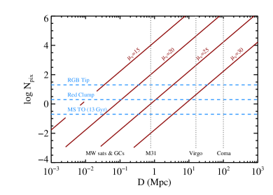
The $N_{\rm pix}$ parameter depends on the distance, surface brightness (which is proportional to the stellar surface density), mass-to-light ratio, and the IMF. Figure 1 shows the relation between $N_{\rm pix}$, distance, and surface brightness. We have assumed a mass-to-light ratio of 4.0 and a mass-to-number ratio of 2.0 in order to convert luminosities into numbers, and a pixel resolution element of $0.05\arcsec$ (i.e., the pixel scale of ACS). Also shown in this figure is the approximate crowding limit for three important stellar phases: the main sequence turn-off at 13 Gyr, the red clump, and the tip of the red giant branch (RGB). Above these limits in $N_{\rm pix}$ the phases are crowding limited, which means that stars in this phase, and fainter, cannot be reliably separated from the background. Distances to a variety of stellar systems including Milky Way satellite galaxies and globular clusters (GCs), M31, and the Virgo and Coma clusters are included at the bottom of the figure. As mentioned in the Introduction, most of the next-generation facilities, including WFIRST and JWST, will not deliver significant improvements in spatial resolution compared to HST, and so we can expect the landscape depicted in Figure 1 to remain largely unchanged for the next $10-20$ years.

Figure 1.— Relation between the mean number of stars per pixel, $N_{\rm pix}$, distance, and surface brightness for a pixel scale of 0.05″and a resolution element of 10 pixels. Also shown are the approximate crowding limits for three key stellar phases: the oldest main sequence turnoff (MS TO), the red clump, and the tip of the RGB. Approximate locations of a variety of objects are included at the bottom of the figure. The intersection between the dashed and solid lines marks the region above which that particular stellar phase is crowding limited. For example, at the distance of M31, regions with a surface brightness of 25 mag arcsec^-2 fully resolve the RGB tip, barely resolve the red clump, and do not resolve the MS TO.

3. Pixel Color Magnitude Diagrams

Figure 2.— Model images and pCMDs as a function of the number of stars per pixel, $N_{\rm pix}$. All models adopt a solar metallicity, 10 Gyr stellar population (shown as a grey line in each pCMD to guide the eye). Simulated pCMDs contain $1024^{2}$ pixels; $400^{2}$ pixel subregions are shown in the PSF-convolved images in the left panels. Middle and right panels show the resulting pCMDs without and with convolution with the HST ACS F814W PSF. The pCMDS are displayed as Hess diagrams with a logarithmic color mapping. Horizontal dashed lines in the right panels mark the approximate crowding limit, above which PSF photometry is possible. In the upper right panel, blue symbols denote what would be recoverable from PSF photometry; there are 1062 stars above the crowding limit for $N_{\rm pix}=1$ but none for $N_{\rm pix}\geq 10^{2}$.

3.1. Methods

pCMDs are constructed by simply measuring magnitudes within a pixel and plotting those pixel magnitudes in a color magnitude diagram. Obviously this requires the pixels from different images, bands, etc. to be registered to the exact same reference frame and to have the same pixel scale. The modeling of stellar populations in pCMD space is in principle very straightforward. Our goal is to model the image plane, and from that image construct pCMDs. In order to model the image plane we must create stellar populations at each pixel and then convolve the model image with the PSF. At each pixel we draw stars according to weights specified by the product of the IMF, the star formation history (SFH), and the mean number of stars per pixel. The flux of each star can be reddened according to a reddening law. The stars within a pixel are summed together to produce the final spectral energy distribution of the pixel.

In practice we adopt a Salpeter IMF (Salpeter, 1955) with a lower-mass cutoff of $0.08M_{\odot}$ and isochrones from the MIST project (Choi et al., 2016). The SFH is set by weights supplied in 7 age bins and can either be specified non-parametrically or via parametric relations (a constant model or an exponential model with a decay timescale denoted by $\tau_{\rm SF}$). Note that the SFH extends from $10^{6}$ yr to $10^{10}$ yr. We allow for a single reddening parameter, $E(B-V)$, that is applied to all stars equally, with an $R_{V}=3.1$ reddening law from Schlafly & Finkbeiner (2011). Bandpass filters are adopted from the HST ACS camera and for brevity we refer to the HST filters with the following abbreviations: $g_{475}=$F475W and $I_{814}=$F814W. We adopt a single PSF derived from ACS F814W imaging when convolving images (the F475W and F814W PSFs are very similar and so this simplification is unlikely to impact our comparison to observations in later sections).

In most respects the modeling process is similar to modeling resolved stellar populations. However, there are key differences: first, since we are modeling the image plane, we must take into account the PSF in the modeling procedure. Second, computational considerations require us to model a finite image plane, which implies that the model contains a non-trivial stochastic noise component (we return to this point in Section 4). Third, the key variable $N_{\rm pix}$ must be modeled. In reality one might need to consider a distribution function for $N_{\rm pix}$ rather than a single value. A simplifying feature of modeling in pCMD space is that one need not explicitly consider stellar binarity since we are not attempting to resolve individual stars. For these reasons the number of free parameters is not necessarily much larger, although the modeling of populations in pCMD space is substantially more computationally intensive.

Figure 3.— Sensitivity of pCMDs to the star formation history. Solar metallicity models with $N_{\rm pix}=10^{2}$ are shown for four SFHs: a 10 Gyr single-age model, $\tau$-model SFHs with $\tau_{\rm SF}=2$ and 5 Gyr, and a constant SFH. The pCMDS are displayed as Hess diagrams with a logarithmic color mapping. Isochrones at 0.01 and 10 Gyr are shown in grey to guide the eye. There is clear sensitivity to the different age components in these SFHs in the mean color of the faint pixels, the relative numbers of RGB and upper main sequence stars, and the distribution of stars along the upper main sequence.

3.2. Information Content of pCMDs

In this section we illustrate the information content of pCMDs as a function of $N_{\rm pix}$, SFH, and metallicity.

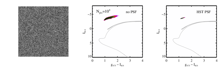
We begin with Figure 2, which shows the image plane and pCMDs as a function of $N_{\rm pix}$ in the $g_{475}$ and $I_{814}$ filters. We show pCMDs both with and without convolution with the PSF in order to illustrate the critical role played by the PSF. Models were generated for solar metallicity 10 Gyr single-age stellar populations with zero reddening. The distribution of points in the pCMD is represented by a Hess diagram with a logarithmic color mapping. Some of the discrete features evident in the top right panel are the result of the finitely-sampled isochrone, PSF and image-plane (by $N_{\rm pix}\gtrsim 10^{2}$ these numerical issues become negligibly small).

One sees clearly from this figure that the morphology in the pCMD varies smoothly from $N_{\rm pix}=1$ to $N_{\rm pix}=10^{4}$, indicating that the information content in these diagrams also varies smoothly. The approximate crowding limit is shown in the PSF-convolved pCMDs in order to underline the rich morphology that lies in the regime that is not included in resolved stellar population analysis. We also show in the top right panel the stars that are recoverable as resolved sources above the crowding limit. By $N_{\rm pix}\geq 10^{2}$ there are no stars in the entire image above the (approximate) crowding limit.

Figure 4.— Same as Figure 3, now for $N_{\rm pix}=10^{4}$.

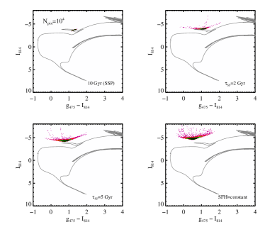
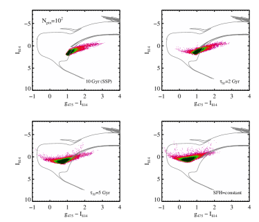
Figures 3 and 4 show the effect of different SFHs in pCMD space for two values of $N_{\rm pix}$. In each figure we compare a single age population at 10 Gyr to two exponentially-declining ($\tau$-model) SFHs with timescales of $\tau_{\rm SF}=2$ and 5 Gyr, and a constant SFH. All models are reddening-free and at solar metallicity. Several important trends are evident. First, there is clearly a varying balance between luminous red and blue pixels, due to the varying influence of upper main sequence and RGB stars. Second, the distribution of stars along the upper main sequence is clearly changing with the SFH. Third, the mean color of the faintest pixels and the faint limit of the faintest pixels also varies with SFH. Also notice that some of the finger-like features extending vertically toward brighter fluxes are the result of one or a few rare bright stars. In pixel space a single bright star will occupy many pixels owing to the effect of the PSF. These pixels will vary in brightness at approximately constant color (depending in detail on the level of similarity of the PSFs of the two filters). In many cases those finger-like structures would be recoverable as resolved sources above the crowding limit.

Figure 5 shows pCMDs as a function of metallicity. Models were generated for a 10 Gyr single-age solar metallicity population with zero reddening. Also shown is a reddening vector assuming the reddening law of Schlafly & Finkbeiner (2011) for a reddening of $E(B-V)=0.3$ and $R_{V}=3.1$. As is well-known, an increase in dust or metallicity will result in redder colors. In unresolved data it is generally impossible to separate the effects of dust, metallicity, and age with a single color. However, with semi-resolved data there is clearly much more information. Notice that while the pCMDs become redder overall with increasing metallicity, the morphology of the data in pCMD space also changes, becoming more horizontally-aligned with increasing metallicity. We therefore expect that pCMDs will enable the disentangling of metallicity and dust effects even when only two imaging bands are available. Though not shown, we have made similar diagrams for $I_{814}-H_{160}$ colors and find an even stronger sensitivity to metallicity, suggesting that optical-NIR colors may be better suited for jointly estimating metallicities and reddening.

Figure 5.— pCMDs as a function of metallicity. Each panel shows a solar metallicity 10 Gyr single-age model displayed as a Hess diagram (color mapping is logarithmic). Also shown is a reddening vector for a standard $R_{V}=3.1$ reddening law and $E(B-V)=0.3$. While both metallicity and reddening result in overall redder colors, the morphology of the pCMD contains a significant amount of metallicity information. For example the pCMDs transition from being more vertically-aligned to more horizontally-aligned with increasing metallicity. It should therefore be possible to separately constrain metallicity and reddening with only two band imaging.

4. Fitting Data in PCMD Space

In this section we describe our approach to fitting data in pCMD space and demonstrate its effectiveness by testing against mock observations.

Figure 6.— SFH recovery tests with mock data. In each panel the recovered SFH (solid line) is compared to the input SFH (dashed line). Upper panels show the recovered SFH and $1\sigma$ errors for mock data with a constant SFH and solar metallicity. The upper left panel shows results for $N_{\rm pix}=10^{2}$ and the upper right panel shows results for $N_{\rm pix}=10^{4}$. In both cases the total mass of the population is fixed, so the total number of pixels in the upper right panel is $100\times$ fewer than in the left. The bottom left panel shows the recovered SFH for an input model with a $\tau-$model SFH with $\tau_{\rm SF}=1$ Gyr. The bottom right panel shows results for a constant SFH with a burst in the second youngest age bin resulting in $5\times$ more mass. Also shown in this panel is a constant SFH (dotted line) for comparison.

4.1. Fitting Technique

The basic framework for fitting observations in pCMD space is as follows. One must simulate an image plane (actually two, one for each band) of some dimension for a given input SFH, reddening, and $N_{\rm pix}$, convolve with the appropriate PSF, add observational errors, bin into a Hess diagram in pCMD space, compute the likelihood of this model given the data, and iterate. We implement this in practice in the following manner. The image plane is simulated at a resolution of $256^{2}$ pixels. The SFH has a free, non-parametric form discretized into 7 age bins with the following boundaries: $(6.0,7.0,8.0,8.5,9.0,9.5,10.0,10.2)$ in units of log age (yr). We assume that the SFR is constant within each bin. The mass in each bin, $M_{i}$, constitutes 7 free parameters ($N_{\rm pix}$ is derived from the integral of the SFH). The reddening is taken to be a single parameter: log $E(B-V)$. The final free parameter is the metallicity, [Z/H]. We fit for a single metallicity by interpolating within the isochrone tables (which include the bolometric corrections). There are thus 9 free parameters in total. The priors on the parameters are flat in log space over the boundaries: [Z/H]$=(-1.1,0.5)$, log $E(B-V)=(-6.0,0.0)$, log $M_{i}/M_{\rm tot}=(-10.0,0.0)$. The lower limit on the metallicity was simply a practical consideration given that we are interested in this paper in metal-rich regions within M31.

The PSF is implemented by dividing the image into 16 subregions. Within each subregion the image is convolved with a PSF that has been shifted by 1/4 of a pixel. We do this because we have assumed in the model that the stellar populations reside at the center of each pixel, whereas in reality the stars can of course fall anywhere in the image plane, not only at pixel centers.

Observational (photon counting) errors are applied to the model by converting the pixel fluxes into counts by specifying a distance to the object of interest and an exposure time. At each pixel we then draw from a Poisson distribution with a mean given by the mean number of counts in each pixel.

The default MIST isochrones are very densely sampled in mass at each age (see Dotter, 2016, for details). In order to ease the computational burden in the fitting we have made use of isochrones that are sampled with $5\times$ fewer equivalent evolutionary points, resulting in $\sim 100-200$ points per isochrone. In testing we have found that this reduction in isochrone points has a very minor effect on the resulting pCMD, mostly affecting the very rare and luminous stars, which in any event do not receive significant weight in the fit.

Errors on both the data and the model Hess diagrams are computed directly from the number of pixels at each point (assuming Poisson statistics). Both the model and data Hess diagrams are normalized to unity.

We begin the fitting procedure by fitting only for $N_{\rm pix}$ and a smooth exponentially-declining SFH specified by $\tau_{\rm SF}$. We fix the reddening to zero and the metallicity to solar. This two parameter fit provides a good starting position for the main fitting routine, which employs the Markov chain Monte Carlo (MCMC) technique emcee (Foreman-Mackey et al., 2013). We use 256 walkers and find that the solution is typically well-converged after $10^{3}$ iterations.

Fitting pCMD data presents several unique challenges not encountered when fitting resolved CMD data. Chief among them is the Poisson nature of drawing stars and populating them in a finite image. For $256^{2}$ image pixels and $N_{\rm iso}\approx 3000$ isochrone points this requires $\sim 10^{8}$ Poisson draws per likelihood call. This is computationally very expensive. Moreover, the stochastic nature of the model implies that the exact same set of parameters will result in a somewhat different model, and hence a different $\chi^{2}$ value. Such a model would require more sophisticated search techniques than standard MCMC. This latter issue could be mitigated by simulating an image of sufficiently large number of pixels, but in our testing even $1024^{2}$ pixels was not sufficient to overcome the Poisson noise. In order to circumvent these two issues (the expense of drawing many Poisson numbers and the stochastic nature of the model), we decided to make the following approximation. Rather than drawing random numbers for the computation of each Poisson draw, we created a fixed set of $256^{2}\times N_{\rm iso}$ random numbers at the beginning of the program. This ensures that each isochrone point has a unique random number at each image pixel, and it also guarantees that the model is deterministic and is computationally faster by about a factor of 3. We then fit each dataset 10 times with a different random number seed and combine the 10 posteriors in an attempt to account for the uncertainties in the model induced by stochastic effects (note that when we generate mock data, we use a random number seed different the 10 used in the fitting).

We make two additional simplifications. We assume that isochrone points with a mass $<0.7M_{\odot}$ or a mean number (which is the product of the IMF and SFH weights) $\langle N\rangle>10^{3}$ contain no pixel-to-pixel variation and hence are not discretely drawn. For the rest, we draw from a Poisson distribution if $\langle N\rangle<100$ and a Gaussian distribution otherwise. With these simplifications each likelihood call takes $\approx 1$ s.

As this is the first attempt to fit observations in pCMD space, we have taken a somewhat simplified approach to fitting the data. Areas for future improvement include the following: 1) exploring techniques for rapidly generating models that do not suffer from stochastic effects, e.g., by simulating images of much larger numbers of pixels; 2) allowing for more metallicity components, either in the form of a metallicity distribution function at a fixed age or the freedom for each age component to have its own metallicity; 3) a dust model characterized by more than a single $E(B-V)$ value, e.g., allowing for a distribution function of reddening values as in Dalcanton et al. (2015); 4) fitting not just $N_{\rm pix}$ but $P(N_{\rm pix})$, i.e., allowing for the fact that a given physical region will in nearly all cases have a distribution of $N_{\rm pix}$ values; 5) a more detailed modeling of the PSF, including e.g., its spatial variation across the image. All of these improvements are straightforward to implement although most will significantly increase the computational expense of each likelihood evaluation.

Figure 7.— Left panels: Comparison between pCMDs of two regions within the bulge of M31 (upper panels) and the corresponding best-fit models (lower panels). The pCMDS are displayed as Hess diagrams with a logarithmic color mapping. The best-fit $N_{\rm pix}$ values are also shown in the legends of the bottom panels. A 10 Gyr solar metallicity isochrone is shown in grey to guide the eye. Right panel: Cumulative SFH derived by fitting the observed pCMD to models. The solid line is offset by 0.05 dex along the x-axis for clarity. Error bars are $1\sigma$ uncertainties. Also shown are several smooth SFHs to guide the eye (dotted lines). The red point with error bars represents the mass fraction and age of the young stellar component reported by Dong et al. (2015) from fitting integrated photometry for a region 0.2 kpc from the center.

4.2. Tests With Mock Data

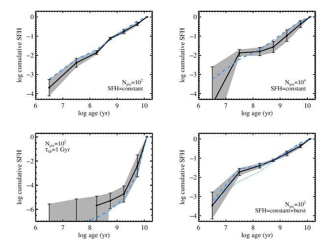
Figure 6 shows the results of several tests of SFH recovery with mock data. The mock data were constructed assuming a solar metallicity population with zero reddening. In each panel the resulting best-fit cumulative SFH is shown as a solid line with the grey bands marking the $1\sigma$ uncertainties. The input SFH is also shown as a dashed line. While we focus here on the SFH recovery, we are simultaneously also fitting for metallicity and dust content. The metallicities are recovered to within 0.05 dex, the reddening is constrained to be $<0.01$, and the overall normalization, $N_{\rm pix}$ is recovered to within 0.1 dex.

In the top panels we fit mock pCMDs generated with a constant SFH for two values of $N_{\rm pix}$. The upper left panel shows a model with $N_{\rm pix}=10^{2}$. The recovered SFH agrees very well with the input value, with statistical uncertainties of less than a factor of two for all age bins except the youngest where the uncertainties are a factor of three. In the upper right panel we show a model with $N_{\rm pix}=10^{4}$ and $100\times$ fewer pixels. In other words, the total mass of the two populations in the top panels are the same. One can think of the top panels as being of the same underlying system with the right panel observed at a distance $10\times$ greater than the left panel. As a consequence, the information content is lower in the right panel compared to the left and the uncertainties are therefore larger. Nonetheless, even at $N_{\rm pix}=10^{4}$ one can reliably recover the full SFH to remarkably high precision.

The bottom left panel shows the result for an old stellar population with an exponential decay time of $\tau_{\rm SF}=1$ Gyr and $N_{\rm pix}=10^{2}$. Here again the best-fit SFH agrees very well with the input model.

The final test is shown in the bottom right panel of Figure 6. Here we take a constant SFH and increase the mass in the second youngest bin by a factor of 5. In other words, the system has an underlying constant SFH with a recent, large burst of star formation. Here again the recovery is excellent, indicating that we can recovery fairly detailed structure in the SFH of crowding-limited systems by analyzing their pCMDs.

Overall we find these tests very encouraging as they imply that we can reliably infer SFHs in a variety of astrophysically interesting regimes including old and young stellar populations and populations with bursty SFHs. It is also encouraging that the best-fit solutions and $1\sigma$ uncertainties encompass the input model in essentially all age bins for all of our tests.

5. Comparison to Observations

Having laid out the basic idea behind pCMDs and demonstrated that one can quantitatively recover SFHs by fitting models to data in pCMD space, we now turn to a comparison with observations. For this purpose we utilize HST observations of M31 obtained through the PHAT survey (Dalcanton et al., 2012). Specifically, we use the brick-level drizzled mosaics available in the MAST archive. We adopt a distance modulus to M31 of 24.47 (McConnachie et al., 2005). In order to simulate the effect of photon noise we adopt an exposure time in the $g_{475}$ and $I_{814}$ bands of 3620s and 3235s, respectively (Dalcanton et al., 2012).

5.1. The Bulge of M31

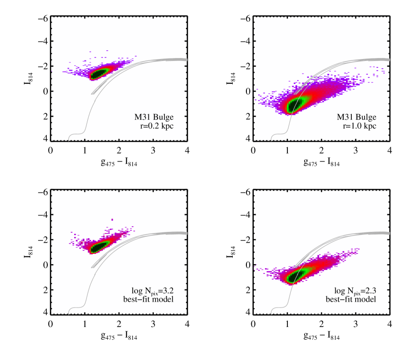
We first consider the old stellar population in the bulge of M31. We selected two regions from Brick 1 spanning a factor of $\approx 10$ in $N_{\rm pix}$. The first region lies $\approx 200$ pc from the center of M31 and has $N_{\rm pix}\sim 10^{3}$ (note that this is well beyond the inner $\sim 10$ pc where a young cluster of blue stars resides; Lauer et al., 2012). The second region lies 1 kpc from the center and has $N_{\rm pix}\sim 10^{2}$. Regions were selected over a relatively narrow range in radius from the center in order to identify groups of pixels that would have a relatively narrow distribution of $N_{\rm pix}$. The first and second regions include 253,000 and 79,000 pixels, respectively. No attempt was made to remove artifacts, clearly resolved bright stars, or other features. Note that the crowding limit is so severe in the bulge of M31 that it is only possible to reliably photometer the most luminous giants based on optical-NIR HST data (Dalcanton et al., 2012; Williams et al., 2014).

Figure 8.— Left panels: Comparison between pCMDs of a small region of the star-forming disk of M31 (upper left) and models with $N_{\rm pix}=10^{1.5}$. This particular region was chosen to coincide with one of the regions used in resolved star CMD fitting (see Figure 9). The models include the best-fit (upper right) and simple, solar metallicity models with a constant SFH and a $\tau$-model SFH (bottom panels). The pCMDs are displayed as Hess diagrams with a logarithmic color mapping. A 10 Gyr solar metallicity isochrone is shown in grey to guide the eye. Right panel: Cumulative SFH derived by fitting the observed pCMD to models. Shaded region represents the $1\sigma$ uncertainties. Also shown are several smooth SFHs to guide the eye (dotted lines).

The left panels of Figure 7 show a comparison of pCMDs between these two regions of the bulge of M31 and the best-fit models. The effect of the PSF and observational (photon counting) uncertainties are included in the models. Overall the best-fit models do a good job of reproducing the features in the observed pCMDs. In detail the observations appear to span a slightly wider range in colors at a fixed luminosity. This may be pointing to the fact that our models are too simplistic. For example, allowing for a metallicity distribution function would result in a broader range of colors at fixed luminosity. We defer these complications to future work.

The right panel of Figure 7 shows the derived cumulative SFHs for these two regions after fitting the observed pCMDs to models. Also shown are simple SFHs to guide the eye. The derived SFHs are steeply declining with time and are broadly consistent with a $\tau-$model SFH with $\tau_{\rm SF}\approx 2$ Gyr. It is also interesting to note that the recovered SFHs are not declining as fast as possible, i.e., a $\tau_{\rm SF}=1$ Gyr model appears to be ruled out by the data. This is noteworthy in light of the integrated light analysis presented in Dong et al. (2015). These authors modelled FUV-NIR photometry in the bulge of M31 and presented evidence for a young stellar population with an age of $\sim 600-800$ Myr and a mass fraction of $\sim 1-2$% in the inner 700 pc. We show their derived age and mass fraction for the young component in the right panel of Figure 7 for their $50-55$″bin, which corresponds closely to our 0.2 kpc region. Their result agrees very well with our derived SFH for this region.

The existence of hot stars associated with old stellar populations (including blue stragglers hot horizontal branch stars, and post-AGB stars) has long complicated the measurement of low levels of SF in such systems, as these hot evolved stars can, in certain circumstances, masquerade as young main sequence stars. Such stars, if present in significant numbers in the bulge of M31, could also bias our derived SFHs high at young and intermediate ages. The most conservative interpretation of our results is that they represent upper limits, as some of the bluest pixels could be due to the hot evolved stars not currently included in our models. We will explore the effect of hot evolved stars on the derived SFHs from pCMDs if future work.

The best-fit metallicities are close to solar and the reddening values are $E(B-V)\lesssim 0.01$. There is some age-dust degeneracy. In light of Figure 5 it would be preferable to use an optical-NIR color in order to more strongly separate these two variables. Nonetheless, the modest degeneracy between age and metallicity does not have a significant impact on the recovery of the SFH.

5.2. The Star-Forming Disk of M31

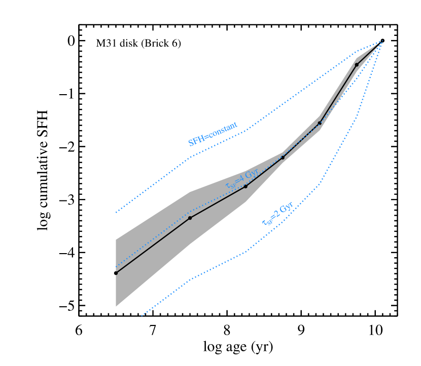
We now consider the stellar population in the star forming disk of M31. For this comparison we selected a single $\approx 100$ pc $\times$ 100 pc region from Brick 6 data. The region corresponds to one of the 9000 regions analyzed by Lewis et al. (2015), who used the resolved stars in this region to constrain the SFH over the past $500$ Myr. The resulting pCMD is shown in the upper left panel of Figure 8. We compare these observed pCMD to three models: the best-fit model, and two simple models. The latter two models are solar metallicity, reddening-free, and have a constant SFH and a $\tau-$model SFH with $\tau_{\rm SF}=2$ Gyr. These simple models were generated with $N_{\rm pix}=10^{1.5}$, which is very close to the best-fit $N_{\rm pix}$ value.

The right panel of Figure 8 shows the derived cumulative SFH for this region. We also show several simple SFHs in order to guide the eye. The derived SFH agrees remarkably well with a smooth exponential model with $\tau_{\rm SF}=4$ Gyr. The best-fit metallicity is close to solar and the reddening is low, $E(B-V)\sim 0.01$.

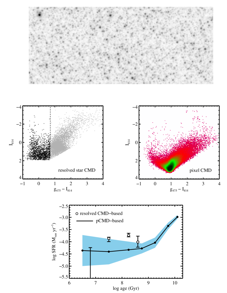
The region that we have analyzed was chosen so that a direct comparison could be made with the resolved star analysis in Lewis et al. (2015). The results are shown in Figure 9. The top panel shows an $I_{814}-$band image of a $40\times 90$ pc subregion of the full $100\times 100$ pc region used in the analysis. The middle panels show the resolved star CMD and the pixel CMD for the full $100\times 100$ pc region. Lewis et al. (2015) fit the region of the resolved CMD blueward of the dotted line in order to focus on the main sequence, which is easier to model than the evolved giants. There are 1800 stars in the fitted region of the diagram. The sharp cutoff at $I_{814}\approx 2$ corresponds to the 50% completeness limit of the resolved star catalog (Lewis et al., 2015).

The derived SFHs from these two approaches are compared in the bottom panel of Figure 9. The resolved star SFH from Lewis et al. is based on modeling the main sequence and hence is limited to the most recent $\approx 500$ Myr; the main sequence turnoff is below the crowding limit for older stellar populations (see Williams et al., 2015, for SFHs derived to older ages in M31 based on modeling the evolved giants). The $1\sigma$ uncertainties on the resolved star SFHs are statistical only; at the youngest age they are dominated by Poisson uncertainties in the number of stars above the crowding limit. The resolved star SFH was re-computed specifically for this comparison for the exact same age bins as the pixel CMDs (courtesy of A. Lewis), and the results were multiplied by 1.5 to convert from a Kroupa (2001) IMF to our adopted Salpeter IMF.

The overall agreement is encouraging. Three of the four age bins agree very well within the errors. The third age bin differs more significantly. In addition to the overall differences in techniques, there are a variety of issues that could drive these differences. First and foremost, we adopt a different set of stellar evolution models than those in Lewis et al. (2015), who adopt the Padova models. It would be interesting to repeat both analysis with a common set of stellar evolution models, as different isochrone tables can induce non-trivial systematics (e.g., Dolphin, 2012; Weisz et al., 2014). Second, Lewis et al. (2015) adopt a more sophisticated dust model than employed herein. They consider a model that allows for a distribution of dust that includes foreground extinction and differential extinction; the extinction PDF is a step function between the foreground and differential extinction values. For this particular region they find a foreground extinction of $E(B-V)=0.1$ (assuming $R_{V}=3.1$) and a differential extinction of $E(B-V)=0.23$. Our best-fit reddening is very low by comparison: $E(B-V)\sim 0.01$. We do not yet know what is responsible for driving our reddening values so low, but it could be related to our simplified treatment of reddening (one value applied to all stars equally). In future work we will explore the more sophisticated dust model employed in Lewis et al. (2015). However, we have tested the impact of our low derived reddening values on the inferred SFH. We re-ran the fitting with a lower limit on the $E(B-V)$ prior of 0.08. The resulting SFRs agree with those shown for our default model in 9 within $1\sigma$ even though the best-fit $E(B-V)$ is closer to 0.1. This test suggests that the derived SFHs are not overly sensitive to the best-fit reddening. Another potential systematic uncertainty is our use of a PSF that does not take into account the effects of the drizzling process that was used to create the final mosaic images.

As a further test of the pCMD-based results, we have used our best-fit parameters to predict the integrated fluxes within this region from the FUV through NIR. For the F475W, F814W, F110W, and F160W filters our predicted fluxes agree to within 3%, 8%, 13%, and 15%, respectively. We have also synthesized FUV and NUV fluxes from GALEX images and find that our predicted fluxes are about a factor of 3 too bright. If we adopt a reddening of $E(B-V)=0.13$ then the model and observed fluxes are in much better agreement, providing additional support to the conclusion that our best-fit reddening values are too low.

Finally, we note that the metallicities derived in the two techniques agree well and both return metallicities within $\approx 0.05$ dex of solar.

We summarize this comparison by concluding that the broad agreement between the resolved star and pCMD-based fitting for the SFH and metallicity is encouraging, but that our model for dust is likely too simplistic. Preliminary tests suggest that this shortcoming does not unduly bias our derived SFH but further tests are needed.

Figure 9.— Direct comparison between resolved and pixel CMDs, and SFHs derived therefrom. Top panel: $I_{814}-$band image of a $40\times 90$ pc subregion of the full $100\times 100$ pc region used in the analysis. Middle left panel: CMD of resolved sources. The resolved sources are truncated at $I_{814}\approx 2$ which corresponds to the 50% completeness limit of the catalog (fainter stars are crowding-limited). Stars redder than the dotted line were excluded from the resolved star CMD analysis in Lewis et al. (2015). Middle right panel: Pixel CMD, represented as a Hess diagram with a logarithmic color map. Bottom panel: SFHs derived from the resolved star CMD (points) and from the pCMD (solid line). The shaded region and error bars represent $1\sigma$ uncertainties. The resolved star SFH was modeled with the exact same age binning used for the pCMD-based SFHs. The overall agreement is encouraging given the different systematic uncertainties between the two techniques. The resolved CMD-based SFH was derived from fitting the main sequence and so is limited to younger ages because the main sequence turnoff point for older ages is below the crowding limit.

6. Discussion

We envision pCMDs being employed in at least two related but distinct regimes. First, in the regime where resolved photometry is not possible even for the brightest stars, pCMDs offers a unique opportunity to extract stellar population information. We presented one example here for the bulge of M31. Other examples include more distant systems (e.g., massive galaxies in the Virgo cluster). As we have remarked earlier, the pCMD concept is in some sense a generalization of the SBF technique, which has been used both as a distance indicator and as a probe of stellar populations (e.g., Tonry et al., 2001; Cantiello et al., 2005; Blakeslee et al., 2010). By analogy with the SBF technique, one could imagine including distance as an additional free parameter when fitting pCMDs. Distance results in an overall vertical shift in the pCMD, and no other parameter induces a similar vertical shift in the pCMD. For this reason we anticipate that pCMDs will deliver strong constraints on the distance.

Second, in the regime in which bright stars are resolvable but the oldest main sequence turnoff point remains below the crowding limit, as is the case in the optical-NIR throughout the disk of M31, pCMDs offer a valuable complementary tool that can be used in combination with classic resolved star techniques. In this regime the key point is that for a given age, if the crowding limit is above the turnoff point then there is additional age information in between the crowding limit and the turnoff point that is not used in traditional resolved star analysis but is contained in pCMDs. For example, Williams et al. (2007) used the surface brightness below the magnitude limit of their resolved star data to place additional constraints on the SFH of intracluster stars in the Virgo cluster. As an example of the possible synergy between resolved star and pCMD analyses, the dust model from the resolved star analysis as a prior on the dust model in the pCMD analysis. Ultimately, one could imagine jointly fitting the resolved CMD and pCMD data within the same model, thereby providing the strongest possible constraints on physical parameters of the system.

We emphasize that pCMDs provide a much less obstructed view of the main sequence than is available from standard integrated light observations. For example, for an old stellar population viewed in integrated light, the main sequence comprises $50-60$% of the light at $0.5-0.6\mu m$, and $\approx 30$% at $0.8\mu m$ (e.g., Conroy, 2013). We computed similar numbers for our pCMDs as a function of pixel luminosity, for the case of a $\tau_{\rm SF}=1$ Gyr SFH and $N_{\rm pix}=10^{2}$. At the faintest pixels ($I_{814}\approx 2$), the main sequence contributes 80% of the flux at $0.8\mu m$. The key point is that the pCMDs are sensitive both to the evolved giants and to the sea of main sequence stars, and with pCMDs we can separately extract the age and metallicity-sensitive information from these components. Moreover, by combining pCMDs with spectroscopy at the pixel level one can hope to extract even more information (e.g., Mould, 2012; van Dokkum et al., 2014).

The majority of ground and space-based facilities coming online in the next two decades will not deliver substantially increased angular resolution compared to current facilities, and as a consequence they will not improve upon the crowding limit offered by HST. The ELTs do offer the hopes of dramatically increased angular resolution. In this case many more galaxies will be in the semi-resolved regime (e.g., the central regions of galaxies in the Virgo cluster). In light of this, we believe that one must embrace crowding-limited data and develop tools for extracting information in that regime. pCMDs offer one such example in this direction.

This is the first attempt to fit observations in pCMD space, and, as a consequence, a number of simplifying assumptions have been made. Due to computational limitations we have made several shortcuts; we are optimistic that solutions to these limitations can be found in the near future. Our underlying model is relatively simple, containing only 9 parameters (7 for the SFH, and one each for metallicity and reddening). Clearly the reddening model is too simplistic and it should be straightforward to expand this component into something that rivals the resolved star analysis in sophistication (see e.g., Dalcanton et al., 2015, for the current state of the art). Likewise for the metallicity, in principle it is straightforward to add more components, but in this case the computational burden increases linearly with each added component. Greater care needs to be taken in handling the (spatially variable) PSF. The relative simplicity of the model also suggests that our quoted uncertainties are likely lower limits. Nonetheless, there are no obvious “show stoppers” in the modeling of pCMDs, and so we encourage their use for interpreting crowding-limited data.

7. Summary

We have presented the concept of pixel color magnitude diagrams (pCMDs) as a powerful tool for analyzing stellar populations in the crowding-limited regime. We constructed stellar population models and highlighted the main dependencies on the key parameters. We also compared the model pCMDs to HST imaging of M31 obtained through the PHAT survey. We now summarize our main results.

• A key parameter governing the behavior of pCDMs is the mean number of stars per pixel, $N_{\rm pix}$. This parameter governs how mottled or smooth the image appears, and when combined with the measured flux, can provide a strong constraint on the distance to the system. This is not surprising as the “magnitude” part of pCMDs is essentially equivalent to the information contained in SBFs.

• pCMDs show strong sensitivity to the underlying SFH with the ability to resolve bursts of star formation and place strong constraints on old stellar populations even when the data are strongly crowding-limited. Our simulations have demonstrated that one can recover at least 7 age components non-parametrically with only two filter data.

• In addition to the SFH, the metallicity and dust content can also be reliably separated with pCMDs, especially with optical-NIR colors. While both metallicity and dust result in redder colors, the detailed structure of the data in pCMD space offers strong, separable constraints on both the metallicity and the overall reddening. Again, all of this can be measured with only two filter data.

• We have developed machinery to fit model pCMDs to observations. We then constructed pCMDs from HST imaging of M31 in several small regions in the bulge and disk. We derived non-parametric SFHs in these regions extending from $10^{6}$ yr to $10^{10}$ yr. These are the strongest constraints to-date on the full SFH in the bulge of M31.

• We also compared our SFHs to those derived from fitting the resolved star CMD in one disk field and found overall good agreement for ages $10^{6.5}-10^{8.7}$ yr, where the resolved star results were available. The comparison revealed notable disagreement in the derived reddening, suggesting that there are important systematic uncertainties in our current approach to fitting pCMDs. Going forward, the combination of resolved star and pCMD data should provide the strongest possible constraints on the full SFH.

References

- Beerman et al. (2012) Beerman, L. C. et al. 2012, ApJ, 760, 104
- Blakeslee et al. (2010) Blakeslee, J. P., Cantiello, M., Mei, S., Côté, P., Barber DeGraaff, R., Ferrarese, L., Jordán, A., Peng, E. W., Tonry, J. L., & Worthey, G. 2010, ApJ, 724, 657
- Cantiello et al. (2005) Cantiello, M., Blakeslee, J. P., Raimondo, G., Mei, S., Brocato, E., & Capaccioli, M. 2005, ApJ, 634, 239
- Choi et al. (2016) Choi, J. et al. 2016, ApJ submitted
- Condon (1974) Condon, J. J. 1974, ApJ, 188, 279
- Conroy (2013) Conroy, C. 2013, ARA&A, 51, 393
- Conroy et al. (2015) Conroy, C., van Dokkum, P. G., & Choi, J. 2015, Nature, 527, 488
- Dalcanton et al. (2012) Dalcanton, J. J. et al. 2012, ApJS, 200, 18
- Dalcanton et al. (2015) —. 2015, ApJ, 814, 3
- Dolphin (2002) Dolphin, A. E. 2002, MNRAS, 332, 91
- Dolphin (2012) —. 2012, ApJ, 751, 60
- Dong et al. (2015) Dong, H., Li, Z., Wang, Q. D., Lauer, T. R., Olsen, K. A. G., Saha, A., Dalcanton, J. J., & Williams, B. F. 2015, MNRAS, 451, 4126
- Dotter (2016) Dotter, A. 2016, ApJS, 222, 8
- Foreman-Mackey et al. (2013) Foreman-Mackey, D., Hogg, D. W., Lang, D., & Goodman, J. 2013, PASP, 125, 306
- Greggio et al. (2012) Greggio, L., Falomo, R., Zaggia, S., Fantinel, D., & Uslenghi, M. 2012, PASP, 124, 653
- Hogg (2001) Hogg, D. W. 2001, AJ, 121, 1207
- Kroupa (2001) Kroupa, P. 2001, MNRAS, 322, 231
- Lauer et al. (2012) Lauer, T. R., Bender, R., Kormendy, J., Rosenfield, P., & Green, R. F. 2012, ApJ, 745, 121
- Lewis et al. (2015) Lewis, A. R. et al. 2015, ApJ, 805, 183
- McConnachie et al. (2005) McConnachie, A. W., Irwin, M. J., Ferguson, A. M. N., Ibata, R. A., Lewis, G. F., & Tanvir, N. 2005, MNRAS, 356, 979
- Mould (2012) Mould, J. 2012, ApJ, 755, L14
- Oke & Gunn (1983) Oke, J. B. & Gunn, J. E. 1983, ApJ, 266, 713
- Olsen et al. (2003) Olsen, K. A. G., Blum, R. D., & Rigaut, F. 2003, AJ, 126, 452
- Renzini (1998) Renzini, A. 1998, AJ, 115, 2459
- Salpeter (1955) Salpeter, E. E. 1955, ApJ, 121, 161
- Scheuer (1957) Scheuer, P. A. G. 1957, Proceedings of the Cambridge Philosophical Society, 53, 764
- Schlafly & Finkbeiner (2011) Schlafly, E. F. & Finkbeiner, D. P. 2011, ApJ, 737, 103
- Schreiber et al. (2014) Schreiber, L., Greggio, L., Falomo, R., Fantinel, D., & Uslenghi, M. 2014, MNRAS, 437, 2966
- Tolstoy et al. (2009) Tolstoy, E., Hill, V., & Tosi, M. 2009, ARA&A, 47, 371
- Tonry & Schneider (1988) Tonry, J. & Schneider, D. P. 1988, AJ, 96, 807
- Tonry et al. (2001) Tonry, J. L. et al. 2001, ApJ, 546, 681
- van Dokkum et al. (2014) van Dokkum, P. et al. 2014, ArXiv:1404.4874
- van Dokkum & Conroy (2014) van Dokkum, P. G. & Conroy, C. 2014, ApJ, 797, 56
- Walcher et al. (2011) Walcher, J., Groves, B., Budavári, T., & Dale, D. 2011, Ap&SS, 331, 1
- Weisz et al. (2014) Weisz, D. R. et al. 2014, ApJ, 789, 147
- Williams et al. (2007) Williams, B. F. et al. 2007, ApJ, 656, 756
- Williams et al. (2014) —. 2014, ApJS, 215, 9
- Williams et al. (2015) —. 2015, ApJ, 806, 48