Multihead Multitrack Detection with Reduced-State Sequence Estimation

Bing Fan,  Hemant K. Thapar,  and Paul H. Siegel B. Fan and P. H. Siegel are with the Department of Electrical & Computer Engineering, University of California, San Diego, CA 92093 USA (e-mail: bifan@ucsd.edu; psiegel@ucsd.edu)H. Thapar is with OmniTier Storage (e-mail: hemantkthapar@gmail.com)
Abstract

To achieve ultra-high storage capacity, the data tracks are squeezed more and more on the magnetic recording disks, causing severe intertrack interference (ITI). The multihead multitrack (MHMT) detector is proposed to better combat ITI. Such a detector, however, has prohibitive implementation complexity. In this paper we propose to use the reduced-state sequence estimation (RSSE) algorithm to significantly reduce the complexity, and render MHMT practical. We first consider a commonly used symmetric two-head two-track (2H2T) channel model. The effective distance between two input symbols is redefined. It provides a better distance measure and naturally leads to an unbalanced set partition tree. Different trellis configurations are obtained based on the desired performance/complexity tradeoff. Simulation results show that the reduced MHMT detector can achieve near maximum-likelihood (ML) performance with a small fraction of the original number of trellis states. Error event analysis is given to explain the behavior of RSSE algorithm on 2H2T channel. Search results of dominant RSSE error events for different channel targets are presented. We also study an asymmetric 2H2T system. The simulation results and error event analysis show that RSSE is applicable to the asymmetric channel.

Index Terms:
Shingled Magnetic Recording, Multitrack Multihead Detection, Intertrack Interference, Reduced-State Sequence Estimation

I Introduction

Intertrack interference (ITI), caused by aggressively shrinking the track pitch, is one of the more severe impairments in next generation hard disk drives (HDDs) [1][2]. The use of an array reader to simultaneously read and process multiple tracks has recently drawn intensive interest because of its capability to handle ITI as well as electronic noise [3][4]. The associated maximum likelihood (ML) detector complexity is, however, drastically increased.

Consider a symmetric two-head two-track (2H2T) system described by

[ra(D)rb(D)]=[1ϵϵ1][xa(D)h(D)xb(D)h(D)]+[na(D)nb(D)],delimited-[]superscript𝑟𝑎𝐷superscript𝑟𝑏𝐷delimited-[]1italic-ϵitalic-ϵ1delimited-[]superscript𝑥𝑎𝐷𝐷superscript𝑥𝑏𝐷𝐷delimited-[]superscript𝑛𝑎𝐷superscript𝑛𝑏𝐷\displaystyle\left[\!\begin{array}[]{c}r^{a}(D)\\ r^{b}(D)\end{array}\!\right]=\left[\!\begin{array}[]{c c}1&\epsilon\\ \epsilon&1\end{array}\!\right]\left[\!\begin{array}[]{c}x^{a}(D)h(D)\\ x^{b}(D)h(D)\end{array}\!\right]+\left[\!\begin{array}[]{c}n^{a}(D)\\ n^{b}(D)\end{array}\!\right], (9)

where xa(D)superscript𝑥𝑎𝐷x^{a}(D), xb(D)superscript𝑥𝑏𝐷x^{b}(D) are the data sequences independently recorded on two adjacent tracks a𝑎a and b𝑏b, with xi(D)=Σk=0NxkiDksuperscript𝑥𝑖𝐷superscriptsubscriptΣ𝑘0𝑁superscriptsubscript𝑥𝑘𝑖superscript𝐷𝑘x^{i}(D)=\Sigma_{k=0}^{N}\,x_{k}^{i}D^{k} and xki{1,+1}superscriptsubscript𝑥𝑘𝑖11x_{k}^{i}\in\{-1,+1\} for i{a,b}𝑖𝑎𝑏i\in\{a,b\}. Each single track is equalized to the same target h(D)=h0+h1D++hνDν𝐷subscript0subscript1𝐷subscript𝜈superscript𝐷𝜈h(D)=h_{0}+h_{1}D+\dots+h_{\nu}D^{\nu}, and the ITI effect is characterized by a parameter ϵitalic-ϵ\epsilon. The received sequences from two heads, ra(D)superscript𝑟𝑎𝐷r^{a}(D) and rb(D)superscript𝑟𝑏𝐷r^{b}(D), include additive electronic noise, na(D)superscript𝑛𝑎𝐷n^{a}(D) and nb(D)superscript𝑛𝑏𝐷n^{b}(D). We assume na(D)superscript𝑛𝑎𝐷n^{a}(D) and nb(D)superscript𝑛𝑏𝐷n^{b}(D) are uncorrelated and i.i.d, with nka,nkb𝒩(0,σ2)similar-tosuperscriptsubscript𝑛𝑘𝑎superscriptsubscript𝑛𝑘𝑏𝒩0superscript𝜎2n_{k}^{a},n_{k}^{b}\sim{\cal N}(0,\sigma^{2}).

The corresponding ML detector simultaneously decodes two tracks by searching a joint trellis [5][6][7]. Let 𝒙k=(xka,xkb)subscript𝒙𝑘superscriptsubscript𝑥𝑘𝑎superscriptsubscript𝑥𝑘𝑏{\boldsymbol{x}}_{k}=(x_{k}^{a},x_{k}^{b}) denote the k𝑘kth input symbol of the 2H2T system. The possible input symbols form a two dimensional 4-symbol constellation. This extended input set causes exponential increase in the computation complexity. For a channel with memory ν𝜈\nu, the ML trellis has 4νsuperscript4𝜈4^{\nu} states, each with 444 incoming and outgoing edges. Compared to the traditional single-head single-track (SHST) detector with complexity O(2v)𝑂superscript2𝑣O(2^{v}), the ML 2H2T detector operates at O(4ν)𝑂superscript4𝜈O(4^{\nu}). For ν>3𝜈3\nu>3, which is typical in practical recording channels, the ML 2H2T detector becomes impractical.

In this work we consider the design of reduced-complexity detectors while retaining good performance. The underlying idea is to drop less possible paths at early stages. This low complexity algorithm, called reduced-state sequence estimation (RSSE) [8], was first designed for transmitting signals from a large quadrature amplitude modulation (QAM) constellation through a partial response channel with long memory. The RSSE trellis, which was originally constructed based on the Ungerboeck set partition tree, has fewer states, but retains a well-defined structure. Efforts were made to develop similar algorithms for the 2H2T system. The authors of [9] showed a way to design low complexity trellis, but their construction generally suffers from high performance loss. We propose a different approach in this paper. We find that by a simple eigen decomposition, the 2H2T system can be transformed to a QAM-type system, and the reduced-state trellis can be constructed by redefining the distance measure on the transformed input constellation. This new construction rule provides greater flexibility in performance/complexity tradeoffs. Our simulation results show that, with fewer than half the number of the states of the full ML trellis, RSSE can achieve near-ML performance on many channels. This work was partially presented in [10].

Moreover, the evaluation of RSSE performance is tractable through error events analysis. In contrast to the ML detector, some error events in RSSE are merged early due to the reduced-state. An early-merging condition is introduced to identify these error events, and a modified error state diagram is used to search for the dominant early-merged error events. The search results on several reduced-state trellis configurations at different ITI levels are presented. When the minimum distance parameter of the early-merged error events is larger than that of the ML detector, the performance loss of RSSE trellis is almost negligible.

An asymmetric 2H2T system, where the ITI levels sensed by two heads are different, is also considered because of its practical interest. We provide a distance analysis for both the ML detector and the RSSE detector. It is shown that the proposed reduced-state trellis construction rule is also applicable in the asymmetric case.

The paper is organized as follows. In Section II we first briefly review the traditional RSSE algorithm for the QAM system. Next we show how to construct a reduced-state trellis for the 2H2T channel by redefining the distance measure in the input constellation and designing proper set partitioning trees. In Section III we construct different trellis configurations based on the performance/complexity tradeoff, and simulate the RSSE detector on several channels with different channel polynomials. The early-merging condition and error event analysis are presented in Section IV. The dominant error events for several reduced-state trellises on different channels are also tabulated. In Section V we consider to apply the RSSE algorithm to the asymmetric 2H2T model. We present the simulation results as well as error event analysis. The paper is concluded in Section VI.

II 2H2T Detector with RSSE

II-A Review of RSSE

The traditional RSSE is designed for transmitting QAM symbols through an ISI channel with channel memory ν𝜈\nu [8]. Recall that in the ML detector, the trellis state is represented as a length ν𝜈\nu vector,

𝒑n=[𝒙n1,𝒙n2,,𝒙nν],subscript𝒑𝑛subscript𝒙𝑛1subscript𝒙𝑛2subscript𝒙𝑛𝜈\displaystyle{\boldsymbol{p}}_{n}=[\,{\boldsymbol{x}}_{n-1},{\boldsymbol{x}}_{n-2},\dots,{\boldsymbol{x}}_{n-\nu}\,], (10)

where each symbol 𝒙nksubscript𝒙𝑛𝑘{\boldsymbol{x}}_{n-k} is complex-valued, and selected from a two-dimensional signal set 𝒞𝒞{\cal C} whose size is M𝑀M. In RSSE, to reduce the number of trellis states, several ML states are grouped into a subset state. To do this, for the k𝑘kth element 𝒙nksubscript𝒙𝑛𝑘{\boldsymbol{x}}_{n-k} in 𝒑nsubscript𝒑𝑛{\boldsymbol{p}}_{n}, a set partition Ω(k)Ω𝑘\Omega(k) of 𝒞𝒞{\cal C} is defined, and 𝒙nksubscript𝒙𝑛𝑘{\boldsymbol{x}}_{n-k} is represented by its subset index ank(k)subscript𝑎𝑛𝑘𝑘a_{n-k}(k) in Ω(k)Ω𝑘\Omega(k). Notice that Ω(k)Ω𝑘\Omega(k) can be different for k=1,,ν𝑘1𝜈k=1,\cdots,\nu. Let Jk=|Ω(k)|subscript𝐽𝑘Ω𝑘J_{k}=|\Omega(k)| be the number of subsets in partition Ω(k)Ω𝑘\Omega(k), 1JkM1subscript𝐽𝑘𝑀1\leqslant J_{k}\leqslant M. Then the subset index ank(k)subscript𝑎𝑛𝑘𝑘a_{n-k}(k) can take its value from 0,1,,Jk101subscript𝐽𝑘10,1,\cdots,J_{k}-1. The corresponding subset state of 𝒑nsubscript𝒑𝑛{\boldsymbol{p}}_{n} is denoted by

𝒔n=[an1(1),an2(2),,anν(ν)].subscript𝒔𝑛subscript𝑎𝑛11subscript𝑎𝑛22subscript𝑎𝑛𝜈𝜈\displaystyle{\boldsymbol{s}}_{n}=[\,a_{n-1}(1),a_{n-2}(2),\dots,a_{n-\nu}(\nu)\,]. (11)

The trellis constructed from all possible 𝒔nsubscript𝒔𝑛{\boldsymbol{s}}_{n} is called the subset trellis. To obtain a well-defined trellis structure, the partition Ω(k)Ω𝑘\Omega(k) is restricted to be a further partition of the subsets in Ω(k+1)Ω𝑘1\Omega(k+1), for 1kν11𝑘𝜈11\leqslant k\leqslant\nu-1. This condition guarantees that for a given state 𝒔nsubscript𝒔𝑛{\boldsymbol{s}}_{n} and current input 𝒙nsubscript𝒙𝑛{\boldsymbol{x}}_{n}, the next subset state is uniquely determined and represented as

𝒔n+1=[an(1),an1(2),,anν+1(ν)],subscript𝒔𝑛1subscript𝑎𝑛1subscript𝑎𝑛12subscript𝑎𝑛𝜈1𝜈\displaystyle{\boldsymbol{s}}_{n+1}=[\,a_{n}(1),a_{n-1}(2),\dots,a_{n-\nu+1}(\nu)\,], (12)

where an(1)subscript𝑎𝑛1a_{n}(1) is the subset index of 𝒙nsubscript𝒙𝑛{\boldsymbol{x}}_{n} in Ω(1)Ω1\Omega(1), an1(2)subscript𝑎𝑛12a_{n-1}(2) is the index of 𝒙n1subscript𝒙𝑛1{\boldsymbol{x}}_{n-1} in Ω(2)Ω2\Omega(2), and so on. The number of states in the subset trellis is k=1νJksuperscriptsubscriptproduct𝑘1𝜈subscript𝐽𝑘\prod_{k=1}^{\nu}J_{k}. The complexity of a RSSE trellis can be controlled by specifying ν𝜈\nu parameters, Jksubscript𝐽𝑘J_{k} for 1kν1𝑘𝜈1\leqslant k\leqslant\nu. We define the configuration of a subset trellis to be a vector 𝐉=[J1,J2,,Jν]𝐉subscript𝐽1subscript𝐽2subscript𝐽𝜈{\mathbf{J}}=[J_{1},J_{2},\dots,J_{\nu}]. A valid configuration satisfies J1J2Jνsubscript𝐽1subscript𝐽2subscript𝐽𝜈J_{1}\geqslant J_{2}\geqslant\dots\geqslant J_{\nu}.

To apply the Viterbi algorithm (VA) on a subset trellis, a decision feedback scheme is introduced to calculate the branch metric, since the subset state 𝒔nsubscript𝒔𝑛{\boldsymbol{s}}_{n} does not uniquely specify the most recent ν𝜈\nu symbols. During the detection process, a modified path history is used to store the survivor symbol 𝒙^n1subscript^𝒙𝑛1\hat{{\boldsymbol{x}}}_{n-1} that leads to state 𝒔nsubscript𝒔𝑛{\boldsymbol{s}}_{n}. The actual survivor ML state 𝒑^nsubscript^𝒑𝑛\hat{{\boldsymbol{p}}}_{n} is obtained by tracing back ν𝜈\nu steps in the path history. We say that 𝒑^nsubscript^𝒑𝑛\hat{{\boldsymbol{p}}}_{n} is the only one survivor ML state at time n𝑛n among all possible 𝒑nsubscript𝒑𝑛{\boldsymbol{p}}_{n}’s whose corresponding subset state is 𝒔nsubscript𝒔𝑛{\boldsymbol{s}}_{n}. An example will be given in the following section to illustrate this process. Error propagation may occur, but its effect is negligible [8][11].

\dots\dots𝒑n=[𝒙n1,,𝒙nν]subscript𝒑𝑛subscript𝒙𝑛1subscript𝒙𝑛𝜈{\boldsymbol{p}}_{n}=[{\boldsymbol{x}}_{n-1},\dots,{\boldsymbol{x}}_{n-\nu}]𝒑n=[𝒙n1,,𝒙nν]subscriptsuperscript𝒑𝑛subscriptsuperscript𝒙𝑛1subscriptsuperscript𝒙𝑛𝜈{\boldsymbol{p}}^{\prime}_{n}=[{\boldsymbol{x}}^{\prime}_{n-1},\dots,{\boldsymbol{x}}^{\prime}_{n-\nu}]n𝑛nn+1𝑛1n+1n1𝑛1n-1n2𝑛2n-2
(a) ML trellis
\dots\dots𝒔n=[an1(1),,anν(ν)]subscript𝒔𝑛subscript𝑎𝑛11subscript𝑎𝑛𝜈𝜈{\boldsymbol{s}}_{n}=[a_{n-1}(1),\dots,a_{n-\nu}(\nu)]n𝑛nn+1𝑛1n+1n1𝑛1n-1n2𝑛2n-2
(b) Subset trellis
Figure 1: Comparison between the decoding paths on (a) ML trellis and (b) subset trellis. If at time n𝑛n two paths ending at ML states 𝒑nsubscript𝒑𝑛{\boldsymbol{p}}_{n} and 𝒑nsuperscriptsubscript𝒑𝑛{\boldsymbol{p}}_{n}^{\prime} satisfy 𝒙nkank(k)subscript𝒙𝑛𝑘subscript𝑎𝑛𝑘𝑘{\boldsymbol{x}}_{n-k}\in a_{n-k}(k) and 𝒙nkank(k)subscriptsuperscript𝒙𝑛𝑘subscript𝑎𝑛𝑘𝑘{\boldsymbol{x}}^{\prime}_{n-k}\in a_{n-k}(k) for all k=1,,ν𝑘1𝜈k=1,\dots,\nu, then they will merge early at subset state 𝒔nsubscript𝒔𝑛{\boldsymbol{s}}_{n} in the subset trellis. If by time n𝑛n the merged paths are separated by large Euclidean distance, the early merge can be considered to be reliable since the dropped path has a high metric that makes it much less likely to be chosen as the final survivor path.

The underlying idea of RSSE is to drop less likely paths early in the detection process. Since each subset state contains multiple ML states, certain paths will merge earlier in the subset trellis than in the ML trellis, as shown in Fig. 1. If Jk=Msubscript𝐽𝑘𝑀J_{k}=M for 1kν1𝑘𝜈1\leqslant k\leqslant\nu, RSSE becomes MLSE. Otherwise it is suboptimal. To minimize the performance loss, proper set partitions Ω(k)Ω𝑘\Omega(k) should be selected carefully to guarantee that enough distance differences have been accumulated to reliably distinguish between merging paths. For the M𝑀M-QAM system, it is suggested that good performance can generally be obtained by maximizing the minimum intrasubset Euclidean distance for each partition Ω(k)Ω𝑘\Omega(k), k=1,,ν𝑘1𝜈k=1,\cdots,\nu [8]. The Ungerboeck set partition tree [12] is shown to have this property and is adopted to make the selection of Ω(k)Ω𝑘\Omega(k). For more details about the subset trellis construction for the M𝑀M-QAM system, the reader is referred to [8].

The use of the Ungerboeck set partition tree is key to obtaining good performance of the RSSE algorithm on the QAM system. However, such a set partition tree cannot be directly applied to the 2H2T system because of the ITI. In the next subsection we will show that a simple transformation can decompose the original 2H2T system into two independent channels, resulting in a QAM-like structure. Then, instead of using the Euclidean distance, we define a new distance measure between the input symbols, based on which we construct a more suitable set partition tree for the 2H2T system.

II-B Set Partition Tree for 2H2T System

In [13] we show that the 2H2T channel described by equation (9) is equivalent to

[r+(D)r(D)]=[z+(D)h(D)z(D)h(D)]+[n+(D)n(D)],delimited-[]superscript𝑟𝐷superscript𝑟𝐷delimited-[]superscript𝑧𝐷𝐷superscript𝑧𝐷𝐷delimited-[]superscript𝑛𝐷superscript𝑛𝐷\displaystyle\left[\!\begin{array}[]{c}r^{+}(D)\\ r^{-}(D)\end{array}\!\right]=\left[\!\begin{array}[]{c}z^{+}(D)h(D)\\ z^{-}(D)h(D)\end{array}\!\right]+\left[\!\begin{array}[]{c}n^{+}(D)\\ n^{-}(D)\end{array}\!\right], (19)

where

[zk+zk]matrixsubscriptsuperscript𝑧𝑘subscriptsuperscript𝑧𝑘\displaystyle\begin{bmatrix}z^{+}_{k}\\ z^{-}_{k}\end{bmatrix} =[1111][xkaxkb]absentmatrix1111matrixsubscriptsuperscript𝑥𝑎𝑘subscriptsuperscript𝑥𝑏𝑘\displaystyle=\begin{bmatrix}1&1\\ 1&-1\end{bmatrix}\begin{bmatrix}x^{a}_{k}\\ x^{b}_{k}\end{bmatrix} (20)
[rk+rk]matrixsubscriptsuperscript𝑟𝑘subscriptsuperscript𝑟𝑘\displaystyle\begin{bmatrix}r^{+}_{k}\\ r^{-}_{k}\end{bmatrix} =[11+ϵ0011ϵ][1111][rkarkb]absentmatrix11italic-ϵ0011italic-ϵmatrix1111matrixsubscriptsuperscript𝑟𝑎𝑘subscriptsuperscript𝑟𝑏𝑘\displaystyle=\begin{bmatrix}\frac{1}{1+\epsilon}&0\\ 0&\frac{1}{1-\epsilon}\end{bmatrix}\begin{bmatrix}1&1\\ 1&-1\end{bmatrix}\begin{bmatrix}r^{a}_{k}\\ r^{b}_{k}\end{bmatrix} (21)
[nk+nk]matrixsubscriptsuperscript𝑛𝑘subscriptsuperscript𝑛𝑘\displaystyle\begin{bmatrix}n^{+}_{k}\\ n^{-}_{k}\end{bmatrix} =[11+ϵ0011ϵ][1111][nkankb].absentmatrix11italic-ϵ0011italic-ϵmatrix1111matrixsubscriptsuperscript𝑛𝑎𝑘subscriptsuperscript𝑛𝑏𝑘\displaystyle=\begin{bmatrix}\frac{1}{1+\epsilon}&0\\ 0&\frac{1}{1-\epsilon}\end{bmatrix}\begin{bmatrix}1&1\\ 1&-1\end{bmatrix}\begin{bmatrix}n^{a}_{k}\\ n^{b}_{k}\end{bmatrix}. (22)
𝒓^ksubscript^𝒓𝑘\hat{{\boldsymbol{r}}}_{k}rk+subscriptsuperscript𝑟𝑘r^{+}_{k}rksubscriptsuperscript𝑟𝑘r^{-}_{k}𝒓ksubscript𝒓𝑘{\boldsymbol{r}}_{k}𝒓^kT=ΛU𝒓kTsuperscriptsubscript^𝒓𝑘𝑇Λ𝑈superscriptsubscript𝒓𝑘𝑇\hat{{\boldsymbol{r}}}_{k}^{T}=\Lambda U{\boldsymbol{r}}_{k}^{T}Λ=Λabsent\Lambda= [11+ϵ0011ϵ]matrix11italic-ϵ0011italic-ϵ\begin{bmatrix}\begin{smallmatrix}\frac{1}{1+\epsilon}&0\\ 0&\frac{1}{1-\epsilon}\end{smallmatrix}\end{bmatrix} 𝒙ksubscript𝒙𝑘{\boldsymbol{x}}_{k}𝒛ksubscript𝒛𝑘{\boldsymbol{z}}_{k}zk+subscriptsuperscript𝑧𝑘z^{+}_{k}zksubscriptsuperscript𝑧𝑘z^{-}_{k}h(D)𝐷h(D)h(D)𝐷h(D)𝒛kT=U𝒙kTsuperscriptsubscript𝒛𝑘𝑇𝑈superscriptsubscript𝒙𝑘𝑇{\boldsymbol{z}}_{k}^{T}=U{\boldsymbol{x}}_{k}^{T}U=[1111]𝑈matrix1111U=\begin{bmatrix}\begin{smallmatrix}1&1\\ 1&-1\end{smallmatrix}\end{bmatrix} nk+subscriptsuperscript𝑛𝑘n^{+}_{k}1/(1+ϵ)11italic-ϵ1/(1+\epsilon)1/(1ϵ)11italic-ϵ1/(1-\epsilon)nksubscriptsuperscript𝑛𝑘n^{-}_{k}nka+nkbsubscriptsuperscript𝑛𝑎𝑘subscriptsuperscript𝑛𝑏𝑘n^{a}_{k}+n^{b}_{k}nkankbsubscriptsuperscript𝑛𝑎𝑘subscriptsuperscript𝑛𝑏𝑘n^{a}_{k}-n^{b}_{k}
Figure 2: A schematic of the WSSJD model. Coordinate transformations are applied in the input space (𝒛kT=U𝒙kTsuperscriptsubscript𝒛𝑘𝑇𝑈superscriptsubscript𝒙𝑘𝑇{\boldsymbol{z}}_{k}^{T}=U{\boldsymbol{x}}_{k}^{T}) and the output space (𝒓^kT=ΛU𝒓kTsuperscriptsubscript^𝒓𝑘𝑇Λ𝑈superscriptsubscript𝒓𝑘𝑇\hat{{\boldsymbol{r}}}_{k}^{T}=\Lambda U{\boldsymbol{r}}_{k}^{T}). They decompose the original 2H2T system into the sum channel (upper branch) and the subtract channel (lower branch).

Let 𝒙k=(xka,xkb)subscript𝒙𝑘subscriptsuperscript𝑥𝑎𝑘subscriptsuperscript𝑥𝑏𝑘{\boldsymbol{x}}_{k}=(x^{a}_{k},x^{b}_{k}) and 𝒓k=(rka,rkb)subscript𝒓𝑘subscriptsuperscript𝑟𝑎𝑘subscriptsuperscript𝑟𝑏𝑘{\boldsymbol{r}}_{k}=(r^{a}_{k},r^{b}_{k}) be the input and received symbols of the original system (9) and let 𝒛k=(zk+,zk)subscript𝒛𝑘subscriptsuperscript𝑧𝑘subscriptsuperscript𝑧𝑘{\boldsymbol{z}}_{k}=(z^{+}_{k},z^{-}_{k}) and 𝒓^k=(rk+,rk)subscript^𝒓𝑘subscriptsuperscript𝑟𝑘subscriptsuperscript𝑟𝑘\hat{{\boldsymbol{r}}}_{k}=(r^{+}_{k},r^{-}_{k}) denote the input and received symbols of the transformed system (19). Their equivalence is visually indicated in Fig. 2. By applying the coordinate transformations both in the input space and the output space, we decompose the original 2H2T system into two separate channels, both of which are modeled by channel polynomial h(D)𝐷h(D). The noise components of the transformed system, nk+superscriptsubscript𝑛𝑘n_{k}^{+} and nksuperscriptsubscript𝑛𝑘n_{k}^{-}, are independent, but with different noise power, nk+𝒩(0,2σ2(1+ϵ)2)similar-tosubscriptsuperscript𝑛𝑘𝒩02superscript𝜎2superscript1italic-ϵ2n^{+}_{k}\sim{\cal N}(0,\frac{2\sigma^{2}}{(1+\epsilon)^{2}}), nk𝒩(0,2σ2(1ϵ)2)similar-tosubscriptsuperscript𝑛𝑘𝒩02superscript𝜎2superscript1italic-ϵ2n^{-}_{k}\sim{\cal N}(0,\frac{2\sigma^{2}}{(1-\epsilon)^{2}}).

The ML trellis of the transformed system is formed by all possible 𝒑n=[𝒛n1,,𝒛nν]subscript𝒑𝑛subscript𝒛𝑛1subscript𝒛𝑛𝜈{\boldsymbol{p}}_{n}=[{\boldsymbol{z}}_{n-1},\dots,{\boldsymbol{z}}_{n-\nu}]. Notice that in this new trellis the branch labels are independent of ϵitalic-ϵ\epsilon since it only affects the noise power of the sum/subtract channel. The ML detection on this new channel is called weighted sum subtract joint detection (WSSJD), summarized as follows:

  1. 1.

    Calculate r+(D)superscript𝑟𝐷r^{+}(D) and r(D)superscript𝑟𝐷r^{-}(D) using equation (21).

  2. 2.

    To apply VA on the WSSJD trellis, weight the branch metrics

    m(𝒑n,𝒑n+1)𝑚subscript𝒑𝑛subscript𝒑𝑛1\displaystyle m({\boldsymbol{p}}_{n},{\boldsymbol{p}}_{n+1})
    =(1+ϵ)2(rn+yn+)2+(1ϵ)2(rnyn)2,absentsuperscript1italic-ϵ2superscriptsuperscriptsubscript𝑟𝑛superscriptsubscript𝑦𝑛2superscript1italic-ϵ2superscriptsuperscriptsubscript𝑟𝑛superscriptsubscript𝑦𝑛2\displaystyle\quad=(1+\epsilon)^{2}(r_{n}^{+}-y_{n}^{+})^{2}+(1-\epsilon)^{2}(r_{n}^{-}-y_{n}^{-})^{2}, (23)

    where yn+=i=0νhizni+subscriptsuperscript𝑦𝑛superscriptsubscript𝑖0𝜈subscript𝑖subscriptsuperscript𝑧𝑛𝑖y^{+}_{n}=\sum_{i=0}^{\nu}h_{i}z^{+}_{n-i} and yn=i=0νhiznisubscriptsuperscript𝑦𝑛superscriptsubscript𝑖0𝜈subscript𝑖subscriptsuperscript𝑧𝑛𝑖y^{-}_{n}=\sum_{i=0}^{\nu}h_{i}z^{-}_{n-i} are the noiseless ISI channel outputs. Choose the path with the smallest metric and decode to the estimates z^+(D)superscript^𝑧𝐷\hat{z}^{+}(D) and z^(D)superscript^𝑧𝐷\hat{z}^{-}(D).

  3. 3.

    Calculate x^a(D)superscript^𝑥𝑎𝐷\hat{x}^{a}(D) and x^b(D)superscript^𝑥𝑏𝐷\hat{x}^{b}(D) using equation (20).

WSSJD has the same performance as the ML detector [13]. Therefore, in the simulation we use WSSJD as a MLSE substitute for the 2H2T system, and the subset trellis is also constructed by considering the WSSJD inputs/outputs. As we will see, the coordinate transformations in WSSJD make it easier to measure the distances between symbols, which plays an important role in designing the set partition tree. Moreover, the structure of parallel channels can provide additional complexity reduction in selecting survivor paths. However, the applicability of RSSE to the standard 2H2T ML detector holds. With a little abuse of notation, when we mention the “ML trellis”, we refer to the full “WSSJD trellis”. For more information about WSSJD, the reader is referred to [13].

(+2,0)20(+2,0)(2,0)20(-2,0)(0,+2)02(0,+2)(0,2)02(0,-2)z+superscript𝑧z^{+}zsuperscript𝑧z^{-}
(𝒛k,𝒛~k)subscript𝒛𝑘subscript~𝒛𝑘({\boldsymbol{z}}_{k},\tilde{{\boldsymbol{z}}}_{k}) d(𝒛k,𝒛~k)𝑑subscript𝒛𝑘subscript~𝒛𝑘d({\boldsymbol{z}}_{k},\tilde{{\boldsymbol{z}}}_{k})
((+2,0),(2,0))2020((+2,0),(-2,0)) Δ12=8(1+ϵ)2superscriptsubscriptΔ128superscript1italic-ϵ2\Delta_{1}^{2}=8(1+\epsilon)^{2}
((0,+2),(0,2))0202((0,+2),(0,-2)) Δ22=8(1ϵ)2superscriptsubscriptΔ228superscript1italic-ϵ2\Delta_{2}^{2}=8(1-\epsilon)^{2}
((+2,0),(0,+2))2002((+2,0),(0,+2))
((+2,0),(0,2))2002((+2,0),(0,-2)) Δ32=4(1+ϵ2)superscriptsubscriptΔ3241superscriptitalic-ϵ2\Delta_{3}^{2}=4(1+\epsilon^{2})
((2,0),(0,+2))2002((-2,0),(0,+2))
((2,0),(0,2))2002((-2,0),(0,-2))
Figure 3: The input constellation (left) and the ESPDs (right).
Refer to caption
Figure 4: ESPDs as functions of ϵitalic-ϵ\epsilon

The transformations in WSSJD decompose the original 2H2T system into two parallel channels. The sum channel and the subtract channel correspond to transmitting z+(D)superscript𝑧𝐷z^{+}(D) and z(D)superscript𝑧𝐷z^{-}(D) through h(D)𝐷h(D), respectively. Recall that in the QAM system, the real and imaginary components of a complex symbol are also transmitted through the channel independently. Therefore, zk+subscriptsuperscript𝑧𝑘z^{+}_{k} and zksubscriptsuperscript𝑧𝑘z^{-}_{k} can be treated as the real and imaginary components of a complex symbol 𝒛ksubscript𝒛𝑘{\boldsymbol{z}}_{k}. The only difference from the QAM system is that the sum and the subtract channels have different signal-to-noise ratios (SNRs). The sum channel is less noisy, which results in more reliable early merge than the subtract channel. Considering this dimensional asymmetry, instead of using a Euclidean distance we define the effective symbol pair distance (ESPD)

d2(𝒛k,𝒛~k)superscript𝑑2subscript𝒛𝑘subscript~𝒛𝑘\displaystyle d^{2}({\boldsymbol{z}}_{k},\tilde{{\boldsymbol{z}}}_{k})
=(1+ϵ)22(zk+z~k+)2+(1ϵ)22(zkz~k)2.absentsuperscript1italic-ϵ22superscriptsubscriptsuperscript𝑧𝑘subscriptsuperscript~𝑧𝑘2superscript1italic-ϵ22superscriptsubscriptsuperscript𝑧𝑘subscriptsuperscript~𝑧𝑘2\displaystyle\quad=\frac{(1+\epsilon)^{2}}{2}(z^{+}_{k}-\tilde{z}^{+}_{k})^{2}+\frac{(1-\epsilon)^{2}}{2}(z^{-}_{k}-\tilde{z}^{-}_{k})^{2}. (24)
010120312L1subscript𝐿1L_{1},min{Δ22,Δ32}superscriptsubscriptΔ22superscriptsubscriptΔ32\min\{\Delta_{2}^{2},\Delta_{3}^{2}\}L2subscript𝐿2L_{2}, Δ22superscriptsubscriptΔ22\Delta_{2}^{2}L3subscript𝐿3L_{3}, Δ12superscriptsubscriptΔ12\Delta_{1}^{2}L4subscript𝐿4L_{4}
Figure 5: The modified set partition tree. This tree contains 444 levels, {L1,L2,L3,L4}subscript𝐿1subscript𝐿2subscript𝐿3subscript𝐿4\{L_{1},L_{2},L_{3},L_{4}\}, each of which is a set partition of the WSSJD input constellation. The minimum ESPD on each level is specified on the right side. The number associated with each branch is the index of the subset in the corresponding set partition.

The input constellation and the ESPDs between different pairs of symbols are shown in Fig. 3. Notice that ESPDs can change with respect to ϵitalic-ϵ\epsilon, as shown in Fig. 4. Therefore even with the same subset trellis configuration, the RSSE performs differently at different ITI levels.

The set partition tree designed for 2H2T is constructed by maximizing the minimum intrasubset ESPD on each level, which results in an unbalanced tree shown in Fig. 5. Compared to the Ungerboeck set partition tree, the additional level L3subscript𝐿3L_{3} comes from the asymmetric distance measure in the z+superscript𝑧z^{+} and zsuperscript𝑧z^{-} dimensions, and it provides more flexibility in choosing set partitions, which leads to a better performance/complexity tradeoff.

[3,1]31[3,1]\ [3,0]30[3,0]\ [2,1]21[2,1]\ [2,0]20[2,0]\ [1,1]11[1,1]\ [1,0]10[1,0]\ [0,1]01[0,1]\ [0,0]00[0,0]\ 𝒔nsubscript𝒔𝑛{\boldsymbol{s}}_{n}an(1)subscript𝑎𝑛1a_{n}(1){0,1,2,3}0123\{0,1,2,3\}{0,1,2,3}0123\{0,1,2,3\}{0,1,2,3}0123\{0,1,2,3\}{0,1,2,3}0123\{0,1,2,3\}{0,1,2,3}0123\{0,1,2,3\}{0,1,2,3}0123\{0,1,2,3\}{0,1,2,3}0123\{0,1,2,3\}{0,1,2,3}0123\{0,1,2,3\}[3,1]31\ [3,1][3,0]30\ [3,0][2,1]21\ [2,1][2,0]20\ [2,0][1,1]11\ [1,1][1,0]10\ [1,0][0,1]01\ [0,1][0,0]00\ [0,0]𝒔n+1subscript𝒔𝑛1{\boldsymbol{s}}_{n+1}
Figure 6: Subset trellis with configuration [4,2] on memory-2 channel.

When constructing the subset trellis, we choose Ω(k)Ω𝑘\Omega(k) from the levels of the set partition tree for each k=1,,ν𝑘1𝜈k=1,\cdots,\nu, and to guarantee a well-defined trellis structure, Ω(k)Ω𝑘\Omega(k) should always be at the same as or higher level than Ω(k1)Ω𝑘1\Omega(k-1). As an example, Fig. 6 shows an eight-state subset trellis for a memory-2 channel with configuration [4,2]42[4,2], i.e., Ω(1)Ω1\Omega(1) is chosen to be L4subscript𝐿4L_{4}, and Ω(2)Ω2\Omega(2) is chosen to be L2subscript𝐿2L_{2}. In this case, the incoming symbols start to merge at the second stage.

Although one subset state is a group of several ML trellis states, only one ML state can survive inside each subset state at one time slot. Consider the example shown in Fig. 7 and assume ϵ=0.1italic-ϵ0.1\epsilon=0.1. The labels next to the states list the subset states and their current survivor ML states. The labels on the branches are the channel input/output. Notice that the outputs are calculated based on the current 𝒑nsubscript𝒑𝑛{\boldsymbol{p}}_{n}. A look-up table can be stored to facilitate the process of finding the corresponding output labels once the system decides the survivor ML states. Assume the received signals are 𝒓^=(r+,r)=(5,3)^𝒓superscript𝑟superscript𝑟53\hat{{\boldsymbol{r}}}=(r^{+},r^{-})=(5,3). The metric comparison shows that the subset state [0,1]01[0,1] with survivor ML state [(+20),(0+2)]2002\left[\left(\begin{smallmatrix}+2\\ 0\end{smallmatrix}\right),\left(\begin{smallmatrix}0\\ +2\end{smallmatrix}\right)\right] gives the smallest path metric, so the survivor ML state of 𝒔n+1=[0,0]subscript𝒔𝑛100{\boldsymbol{s}}_{n+1}=[0,0] can be decided and updated to be [(+20),(+20)]2020\left[\left(\begin{smallmatrix}+2\\ 0\end{smallmatrix}\right),\left(\begin{smallmatrix}+2\\ 0\end{smallmatrix}\right)\right], which will be used in the next time slot.

[(+20),(20)]2020\left[\left(\begin{smallmatrix}+2\\ 0\end{smallmatrix}\right),\left(\begin{smallmatrix}-2\\ 0\end{smallmatrix}\right)\right][(+20),(0+2)]2002\left[\left(\begin{smallmatrix}+2\\ 0\end{smallmatrix}\right),\left(\begin{smallmatrix}0\\ +2\end{smallmatrix}\right)\right][(20),(+20)]2020\left[\left(\begin{smallmatrix}-2\\ 0\end{smallmatrix}\right),\left(\begin{smallmatrix}+2\\ 0\end{smallmatrix}\right)\right][(20),(0+2)]2002\left[\left(\begin{smallmatrix}-2\\ 0\end{smallmatrix}\right),\left(\begin{smallmatrix}0\\ +2\end{smallmatrix}\right)\right][0,0]00[0,0][0,1]01[0,1][3,0]30[3,0][3,1]31[3,1]𝒔nsubscript𝒔𝑛{\boldsymbol{s}}_{n}𝒑nsubscript𝒑𝑛{\boldsymbol{p}}_{n}(+20)|(00)conditional2000\left(\begin{smallmatrix}+2\\ 0\end{smallmatrix}\right)|\left(\begin{smallmatrix}0\\ 0\end{smallmatrix}\right)(+20)|(44)conditional2044\left(\begin{smallmatrix}+2\\ 0\end{smallmatrix}\right)|\left(\begin{smallmatrix}4\\ 4\end{smallmatrix}\right)(+20)|(40)conditional2040\left(\begin{smallmatrix}+2\\ 0\end{smallmatrix}\right)|\left(\begin{smallmatrix}4\\ 0\end{smallmatrix}\right)(+20)|(04)conditional2004\left(\begin{smallmatrix}+2\\ 0\end{smallmatrix}\right)|\left(\begin{smallmatrix}0\\ 4\end{smallmatrix}\right)[0,0]00[0,0]𝒔nsubscript𝒔𝑛{\boldsymbol{s}}_{n}
Figure 7: An illustration of detection on subset trellis. Consider a subset trellis [4,2]42[4,2] constructed for PR2 channel 1+2D+D212𝐷superscript𝐷21+2D+D^{2}. The leftmost column lists the subset state 𝒔nsubscript𝒔𝑛{\boldsymbol{s}}_{n}, while the column next to it lists the corresponding survivor ML states 𝒑nsubscript𝒑𝑛{\boldsymbol{p}}_{n}. The labels on the branches are formed as in|outconditionalsubscriptinsubscriptout\mathcal{L}_{\text{in}}|\mathcal{L}_{\text{out}}. The branches terminate at subset state 𝒔n+1=[0,0]subscript𝒔𝑛100{\boldsymbol{s}}_{n+1}=[0,0].
0000𝒑^n1=(+20)subscript^𝒑𝑛1matrix20\hat{{\boldsymbol{p}}}_{n-1}=\begin{pmatrix}\begin{smallmatrix}+2\\ 0\end{smallmatrix}\end{pmatrix}(+20)/(+40)matrix20matrix40\begin{pmatrix}\begin{smallmatrix}+2\\ 0\end{smallmatrix}\end{pmatrix}\!/\!\begin{pmatrix}\begin{smallmatrix}+4\\ 0\end{smallmatrix}\end{pmatrix} (20)/(00)matrix20matrix00\begin{pmatrix}\begin{smallmatrix}-2\\ 0\end{smallmatrix}\end{pmatrix}\!/\!\begin{pmatrix}\begin{smallmatrix}0\\ 0\end{smallmatrix}\end{pmatrix}
(a) parallel branches from subset state 0 to 0
11100𝒑^n1=(+20)subscript^𝒑𝑛1matrix20\hat{{\boldsymbol{p}}}_{n-1}=\begin{pmatrix}\begin{smallmatrix}+2\\ 0\end{smallmatrix}\end{pmatrix}(0+2)/(+2+2)matrix02matrix22\begin{pmatrix}\begin{smallmatrix}0\\ +2\end{smallmatrix}\end{pmatrix}\!/\!\begin{pmatrix}\begin{smallmatrix}+2\\ +2\end{smallmatrix}\end{pmatrix} (02)/(+22)matrix02matrix22\begin{pmatrix}\begin{smallmatrix}0\\ -2\end{smallmatrix}\end{pmatrix}\!/\!\begin{pmatrix}\begin{smallmatrix}+2\\ -2\end{smallmatrix}\end{pmatrix}
(b) parallel branches from subset state 0 to 1
Figure 8: Sample parallel branches for subset trellis with 2 states constructed for channel 1+D1𝐷1+D

For a configuration with J1<4subscript𝐽14J_{1}<4, an(1)subscript𝑎𝑛1a_{n}(1) may contain more than one input symbol. For instance, consider the 1+D1𝐷1+D channel. Choosing Ω(1)Ω1\Omega(1) to be L2subscript𝐿2L_{2} or L3subscript𝐿3L_{3} results in a subset trellis with 2 states or 3 states, respectively. For the subset trellis with parallel branches, a pre-selection between the parallel branches is needed during the detection. Due to the symmetric property of WSSJD trellis labels, this pre-selection can be done without explicitly calculating the branch metric, if J1>1subscript𝐽11J_{1}>1. For instance, consider the two scenarios illustrated in Figs. 8. In both cases, the survivor ML state at the starting stage is assumed to be 𝒑^n1=(+2,0)subscript^𝒑𝑛120\hat{{\boldsymbol{p}}}_{n-1}=(+2,0). The input and output labels are marked on the branches. In Fig. 88(a), both the input symbols (+2,0)20(+2,0) and (2,0)20(-2,0) lead the paths to subset state 00. Notice that the input symbols (+2,0)20(+2,0) and (2,0)20(-2,0) have the same value in the zsuperscript𝑧z^{-} dimension, producing the same output on the subtract channel. Instead of calculating metrics from equation (23), the pre-selection performs a thresholding on the sum channel output and make the decision. In this example, the threshold is +22+2, obtained by averaging +44+4 and 00. If rn+>+2superscriptsubscript𝑟𝑛2r_{n}^{+}>+2, the strategy is to pick (+2,0)20(+2,0) as the survived symbol, while for the case rn+<+2superscriptsubscript𝑟𝑛2r_{n}^{+}<+2, (2,0)20(-2,0) should be the survivor Similarly for another case shown in Fig. 88(b), the thresholding is conducted on the subtract channel output, since the two input symbols produce the same output in the sum channel. By comparing rnsuperscriptsubscript𝑟𝑛r_{n}^{-} with the threshold 00, the detector picks (0,+2)02(0,+2) if rn>0superscriptsubscript𝑟𝑛0r_{n}^{-}>0, or (0,2)02(0,-2) if rn<0superscriptsubscript𝑟𝑛0r_{n}^{-}<0. This symmetry property renders the WSSJD formulation preferable over the traditional ML detector.

III Simulation Results

We examine the RSSE performance on various types of channels at different ITI levels. The SNR is defined as

SNR(dB)=10logh(D)22σ2SNR(dB)10superscriptnorm𝐷22superscript𝜎2\displaystyle\text{SNR(dB)}=10\log\frac{\|h(D)\|^{2}}{2\sigma^{2}} (25)
Refer to caption
(a) ϵ=0.1italic-ϵ0.1\epsilon=0.1
Refer to caption
(b) ϵ=0.3italic-ϵ0.3\epsilon=0.3
Figure 9: Performance comparison between RSSE and ML detector on dicide channel at different ITI levels.
Refer to caption
(a) ϵ=0.1italic-ϵ0.1\epsilon=0.1
Refer to caption
(b) ϵ=0.3italic-ϵ0.3\epsilon=0.3
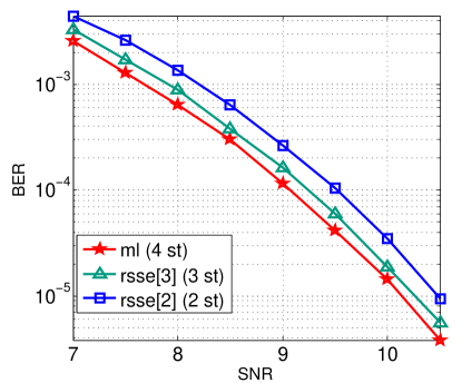
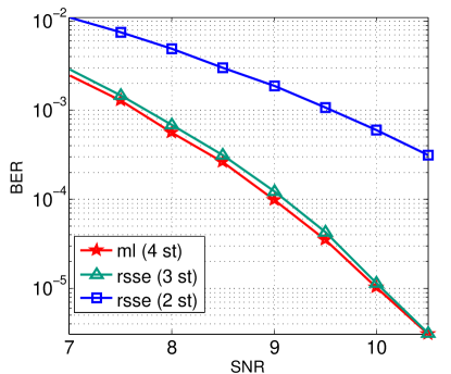
Figure 10: Performance comparison between RSSE and ML detector on PR2 channel at different ITI levels. The legend shows the RSSE subset trellis configuration and the corresponding number of trellis states.
Refer to caption
(a) ϵ=0.1italic-ϵ0.1\epsilon=0.1
Refer to caption
(b) ϵ=0.3italic-ϵ0.3\epsilon=0.3
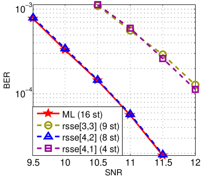
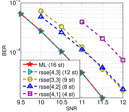
Figure 11: Performance comparison between RSSE and ML detector on EPR4 channel at different ITI levels. The legend shows the RSSE subset trellis configuration and the corresponding number of trellis states.

III-A Dicode Channel

This simple example helps us understand how the pre-selection between parallel branches affects the system. Although early-merging happens at every time step, its doesn’t degrade the performance heavily. From Figs. 9 we see that the performance loss of the 3-state subset trellis is within 0.1dB. The 2 state RSSE performs better under the lower ITI level.

III-B Channel with Higher Memory

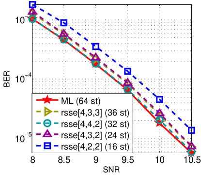
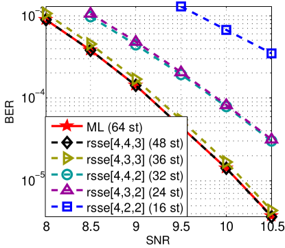
Higher channel memory provides more flexibility to construct the subset trellis, based on different requirements of performance/complexity tradeoff. For the EPR4 channel h(D)=1+DD2D3𝐷1𝐷superscript𝐷2superscript𝐷3h(D)=1+D-D^{2}-D^{3}, we apply RSSE to several subset trellises with different complexities. The resulting bit error rate (BER) vs. SNR performance at different ITI levels is plotted in Fig. 11. The comparison between Figs. 11(a) and Figs. 11(b) shows that even using the same subset trellis, RSSE performs differently under different ITI levels, and its performance correlates with the minimum intrasubset ESPDs of the set partitions configured in the subset trellis. At a low ITI level (ϵ=0.1italic-ϵ0.1\epsilon=0.1), the performance of RSSE on subset trellis [4,4,2]442[4,4,2] coincides with that of the ML detector. The BER curves of [4,3,3]433[4,3,3] and [4,3,2]432[4,3,2] overlap, and are both within 0.1dB from the ML curve. Subset trellis [4,2,2]422[4,2,2] further reduces the number of states to 16, but incurs a 0.3dB loss. When the ITI level becomes higher (ϵ=0.3italic-ϵ0.3\epsilon=0.3), the subset trellis [4,4,2]442[4,4,2] cannot provide reliable early path merging because the minimum intrasubset ESPD Δ22superscriptsubscriptΔ22\Delta_{2}^{2} in Ω(3)=L2Ω3subscript𝐿2\Omega(3)=L_{2} is substantially reduced. However, a less aggressive construction using configuration [4,4,3]443[4,4,3] achieves near-ML performance. The decrease in Δ22superscriptsubscriptΔ22\Delta_{2}^{2} at this ITI level also degrades the performance of RSSE[4,2,2]422[4,2,2] and [4,3,2]432[4,3,2]. Their BER curves overlap in Fig. 11(b). In contrast, the increase of Δ12superscriptsubscriptΔ12\Delta_{1}^{2} brings [4,3,3]433[4,3,3] closer to the ML performance, compared to the case ϵ=0.1italic-ϵ0.1\epsilon=0.1.

Similarly, for the PR2 channel h(D)=1+2D+D2𝐷12𝐷superscript𝐷2h(D)=1+2D+D^{2}, the simulation results in Figs. 10 show that the BER curve of RSSE[4,2]42[4,2] essentially overlaps with that of the ML detector at ϵ=0.1italic-ϵ0.1\epsilon=0.1. For ϵ=0.3italic-ϵ0.3\epsilon=0.3, RSSE[4,3]43[4,3] essentially achieves ML performance.

Trellises ϵitalic-ϵ\epsilon
0.10.10.1 0.20.20.2 0.30.30.3 0.40.40.4
rsse [4,1]41[4,1] 1.25dB 1.3dB 1.35dB 1.2dB
rsse [4,2]42[4,2] 0.1much-less-thanabsent0.1\ll 0.1dB 0.150.150.15dB 0.60.60.6dB 1.11.11.1dB
rsse [3,3]33[3,3] 1.41.41.4dB 0.90.90.9dB 0.60.60.6dB 0.20.20.2dB
rsse [4,3]43[4,3] 0.1much-less-thanabsent0.1\ll 0.1dB
TABLE I: The SNR loss of different subset trellis configurations to achieve BER=104absentsuperscript104=10^{-4} on PR2 channel
Trellises ϵitalic-ϵ\epsilon
0.10.10.1 0.20.20.2 0.30.30.3 0.40.40.4
rsse [4,3,3]433[4,3,3] 0.10.10.1dB 0.1dB 0.05dB 0.1much-less-thanabsent0.1\ll 0.1dB
rsse [4,4,2]442[4,4,2] 0.1much-less-thanabsent0.1\ll 0.1dB 0.150.150.15dB 0.70.70.7dB >1absent1>1dB
rsse [4,3,2]432[4,3,2] 0.10.10.1dB 0.250.250.25dB 0.70.70.7dB >1absent1>1dB
rsse [4,2,2]422[4,2,2] 0.30.30.3dB >1absent1>1dB
rsse [3,3,3]333[3,3,3] >1absent1>1dB 0.70.70.7dB 0.4dB 0.050.050.05dB
rsse [4,3,1]431[4,3,1] >1absent1>1dB
TABLE II: The SNR loss of different subset trellis configurations to achieve BER=104absentsuperscript104=10^{-4} on EPR4 channel

Table I and Table II summarize the performance loss in dB for several subset trellis configurations compared to a ML detector at BER=104absentsuperscript104=10^{-4} on channel PR2 and EPR4, respectively. Several conclusions can be drawn from these tables. First, a trellis with fewer states does not necessarily have a worse performance than the one with more states. For example, in Table II for EPR4 channel, when ϵ=0.1italic-ϵ0.1\epsilon=0.1, the configuration [4,4,2]442[4,4,2] with 32 states outperforms the configuration [4,3,3]433[4,3,3] with 36 states. Second, the performance of one configuration changes drastically at different ITI levels. One example is the RSSE [4,4,2]442[4,4,2], which essentially achieves the ML performance at ϵ=0.1italic-ϵ0.1\epsilon=0.1, but loses over 1dB for ϵ=0.4italic-ϵ0.4\epsilon=0.4. Finally, not all configurations lose more performance at higher ITI. It is interesting to observe that RSSE[3,3,3]333[3,3,3] with parallel branches can have near optimal performance at ϵ=0.4italic-ϵ0.4\epsilon=0.4. Therefore, the pre-selection between parallel branches at every stage is quite realiable. In Section IV we give an explanation of these observations from the view of error events.

III-C Minimum phase channels

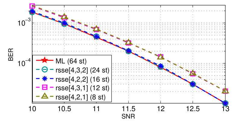
Minimum phase channels can better model the real channel on a disk drive. Assume the transition response of a perpendicular magnetic recording (PMR) disk is s(t)=Vmaxtanh(2t0.579πδ)𝑠𝑡subscript𝑉max2𝑡0.579𝜋𝛿s(t)=V_{\text{max}}\tanh(\frac{2t}{0.579\pi\delta}), where Vmaxsubscript𝑉maxV_{\text{max}} is the writing voltage and δ𝛿\delta indicates the linear density on one data track. By using the whitened matched filter structure in [14], we derive two minimum phase channel polynomials: type 1, h(D)=1+1.6D+1.1D2+0.4D3𝐷11.6𝐷1.1superscript𝐷20.4superscript𝐷3h(D)=1+1.6D+1.1D^{2}+0.4D^{3} for δ=1.3𝛿1.3\delta=1.3, and type 2, h(D)=1+1.9D+1.6D2+0.8D3+0.3D4𝐷11.9𝐷1.6superscript𝐷20.8superscript𝐷30.3superscript𝐷4h(D)=1+1.9D+1.6D^{2}+0.8D^{3}+0.3D^{4} for δ=1.5𝛿1.5\delta=1.5. These are two commonly used densities in current commercial HDDs. Since the minimum phase condition implies that most of the channel energy is distributed over the most recent samples, the early merge in RSSE can be more reliable compared to the linear phase channel (such as PR2 and EPR4 channel). It is interesting to compare type 1 channel with EPR4, both of which have memory ν=3𝜈3\nu=3. As shown in Fig. 12(a), ML, RSSE[4,3,2]432[4,3,2], and RSSE[4,2,2]422[4,2,2] have essentially identical performance. In particular, RSSE[4,2,2]422[4,2,2] performs much better on the minimum phase channel than on the EPR4 channel (Fig. 11(a)), allowing RSSE to achieve near-ML performance with only 16 states. That’s only 25% of the original trellis states. Other more aggressive configurations are also plotted. As can be seen, RSSE with only 8 states can achieve performance that is within 0.3dB of ML detection.

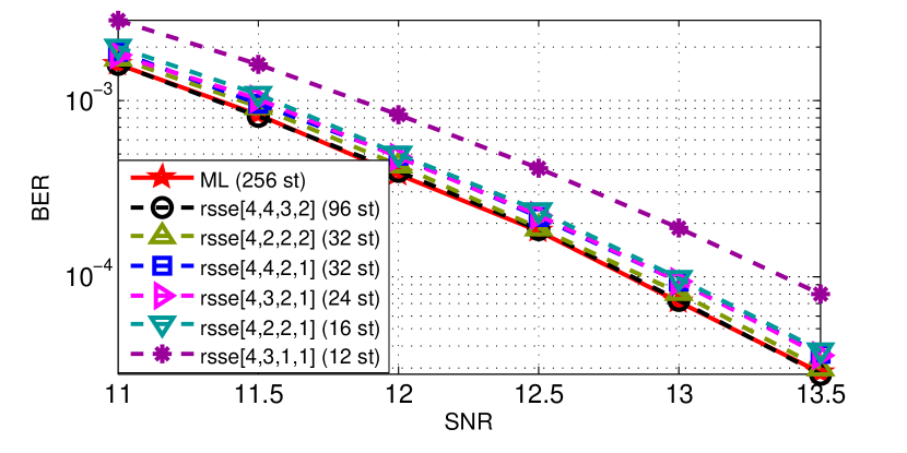
For the type 2 channel which has higher memory, the RSSE algorithm performs even better as in Fig. 12(b). It shows that RSSE[4,2,2,2]4222[4,2,2,2] with 32 states can achieve near-ML performance. That’s 12.5% of the ML trellis states. If 0.1dB loss is permissible, RSSE[4,2,2,1]4221[4,2,2,1] can be used. So the complexity further drops to 6.25% of the original ML algorithm.
Refer to caption
(a) δ=1.3𝛿1.3\delta=1.3
Refer to caption
(b) δ=1.5𝛿1.5\delta=1.5
Figure 12: Performance comparison between RSSE and ML detector on minimum phase channels at ϵ=0.1italic-ϵ0.1\epsilon=0.1. The polynomials are (a) h(D)=1+1.6D+1.1D2+0.4D3𝐷11.6𝐷1.1superscript𝐷20.4superscript𝐷3h(D)=1+1.6D+1.1D^{2}+0.4D^{3}, (b) h(D)=1+1.9D+1.6D2+0.8D3+0.3D4𝐷11.9𝐷1.6superscript𝐷20.8superscript𝐷30.3superscript𝐷4h(D)=1+1.9D+1.6D^{2}+0.8D^{3}+0.3D^{4}.

IV Error Event Analysis

We will use error event analysis to study the performance-complexity tradeoff among different subset trellis configurations.

An error event, 𝒆(D)=𝒛(D)𝒛^(D)𝒆𝐷𝒛𝐷^𝒛𝐷{\boldsymbol{e}}(D)={\boldsymbol{z}}(D)-\hat{{\boldsymbol{z}}}(D), happens if the estimated sequence 𝒛^(D)^𝒛𝐷\hat{{\boldsymbol{z}}}(D) is different from the transmisted sequence 𝒛(D)𝒛𝐷{\boldsymbol{z}}(D). It is well-known [14] that at high SNR, the error event probability of a trellis-based detector can be approximated by PecQ(dmin2σ)subscript𝑃𝑒𝑐𝑄subscript𝑑min2𝜎P_{e}\approx c\cdot Q(\frac{d_{\text{min}}}{2\sigma}), where Q()𝑄Q(\cdot) is the area under the tail of the standard Gaussian distribution.

dmin2=min𝒆(D)d2(𝒆(D))subscriptsuperscript𝑑2minsubscript𝒆𝐷superscript𝑑2𝒆𝐷\displaystyle d^{2}_{\text{min}}=\min_{{\boldsymbol{e}}(D)}d^{2}({\boldsymbol{e}}(D)) (26)

is the minimum distance parameter, and c𝑐c is a coefficient indicating the average number of error events at distance dmin2subscriptsuperscript𝑑2mind^{2}_{\text{min}}. Due to the exponential nature of the Q𝑄Q function, the performance comparison between two detectors can be easily conducted by considering their minimum distance parameter. The error events that lead to dmin2subscriptsuperscript𝑑2mind^{2}_{\text{min}} are called dominant error events.

For the WSSJD detector, due to the unequally scaled noise power, an effective distance measure of a given error event 𝒆(D)=[e+(D),e(D)]𝒆𝐷superscript𝑒𝐷superscript𝑒𝐷{\boldsymbol{e}}(D)=[e^{+}(D),e^{-}(D)] is defined by

dML2(𝒆(D))subscriptsuperscript𝑑2ML𝒆𝐷\displaystyle d^{2}_{\text{ML}}({\boldsymbol{e}}(D))
=(1+ϵ)22e+(D)h(D)2+(1ϵ)22e(D)h(D)2.absentsuperscript1italic-ϵ22superscriptnormsuperscript𝑒𝐷𝐷2superscript1italic-ϵ22superscriptnormsuperscript𝑒𝐷𝐷2\displaystyle=\frac{(1+\epsilon)^{2}}{2}\|e^{+}(D)h(D)\|^{2}+\frac{(1-\epsilon)^{2}}{2}\|e^{-}(D)h(D)\|^{2}. (27)

Comparing equation (24) to equation (27), we can see that ESPD is proportional to the distance parameter of a single error symbol with ek+=zk+z~k+subscriptsuperscript𝑒𝑘subscriptsuperscript𝑧𝑘subscriptsuperscript~𝑧𝑘e^{+}_{k}=z^{+}_{k}-\tilde{z}^{+}_{k} and ek=zkz~ksubscriptsuperscript𝑒𝑘subscriptsuperscript𝑧𝑘subscriptsuperscript~𝑧𝑘e^{-}_{k}=z^{-}_{k}-\tilde{z}^{-}_{k}. Recall that the set partition tree is constructed such that Δ12,Δ22superscriptsubscriptΔ12superscriptsubscriptΔ22\Delta_{1}^{2},\Delta_{2}^{2} and Δ32superscriptsubscriptΔ32\Delta_{3}^{2} are the minimum ESPD on each level from the bottom to the top, and Δ12,Δ22superscriptsubscriptΔ12superscriptsubscriptΔ22\Delta_{1}^{2},\Delta_{2}^{2}, Δ32superscriptsubscriptΔ32\Delta_{3}^{2} are varying with respect to ϵitalic-ϵ\epsilon. Therefore, the minimum distance parameter of the reduced-state trellis configuration also changes with ϵitalic-ϵ\epsilon, and its trend can be roughly predicted by analyzing the change of minimum ESPD in each Ω(k)Ω𝑘\Omega(k). We will give a more detail insights in the following subsections. The minimum value of dML2(𝒆(D))subscriptsuperscript𝑑2ML𝒆𝐷d^{2}_{\text{ML}}({\boldsymbol{e}}(D)) is abbreviated to dmin2superscriptsubscript𝑑min2d_{\text{min}}^{2}, which is the minimum distance parameter of the 2H2T ML detector. It serves as a benchmark for evaluating the performance loss of RSSE algorithm.

IV-A Parallel Branches

If J1<4subscript𝐽14J_{1}<4, the subset trellis contains parallel branches. So early merge happens at every time instant. Ignoring the error propagation effect, we assume that at time k𝑘k, both the correct and the estimated sequences are at state 𝒔ksubscript𝒔𝑘{\boldsymbol{s}}_{k}, and 𝒛ki=𝒛^kisubscript𝒛𝑘𝑖subscript^𝒛𝑘𝑖{\boldsymbol{z}}_{k-i}=\hat{{\boldsymbol{z}}}_{k-i} for all i=1,,ν𝑖1𝜈i=1,...,\nu. At time k+1𝑘1k+1, if 𝒙k,𝒙^kak(1)subscript𝒙𝑘subscript^𝒙𝑘subscript𝑎𝑘1{\boldsymbol{x}}_{k},\hat{{\boldsymbol{x}}}_{k}\in a_{k}(1), the detector needs to decide a survivor symbol, and discard the other one. If the correct symbol is discarded, this wrong decision can not be reversed in the remaining detection steps. The probability of making a wrong decision in the parallel branch selection is Q(h0d(𝒛k,𝒛^k)2σ)𝑄subscript0𝑑subscript𝒛𝑘subscript^𝒛𝑘2𝜎Q(\frac{h_{0}d({\boldsymbol{z}}_{k},\hat{{\boldsymbol{z}}}_{k})}{2\sigma}), where d(𝒛k,𝒛^k)𝑑subscript𝒛𝑘subscript^𝒛𝑘d({\boldsymbol{z}}_{k},\hat{{\boldsymbol{z}}}_{k}) is the square-root of ESPD between 𝒛ksubscript𝒛𝑘{\boldsymbol{z}}_{k} and 𝒛^ksubscript^𝒛𝑘\hat{{\boldsymbol{z}}}_{k}. Let E1subscript𝐸1E_{1} be the set of all such length-1 error events due to the parallel branches. Then, 𝒆kE1subscript𝒆𝑘subscript𝐸1{\boldsymbol{e}}_{k}\in E_{1} if and only if there exist two input symbols 𝒛k,𝒛^kak(1)subscript𝒛𝑘subscript^𝒛𝑘subscript𝑎𝑘1{\boldsymbol{z}}_{k},\hat{{\boldsymbol{z}}}_{k}\in a_{k}(1) such that 𝒆k=𝒛k𝒛^ksubscript𝒆𝑘subscript𝒛𝑘subscript^𝒛𝑘{\boldsymbol{e}}_{k}={\boldsymbol{z}}_{k}-\hat{{\boldsymbol{z}}}_{k}. It can be shown that

dmin2(E1)=min𝒆kE1(1+ϵ)22(h0ek+)2+(1ϵ)22(h0ek)2superscriptsubscript𝑑min2subscript𝐸1subscriptsubscript𝒆𝑘subscript𝐸1superscript1italic-ϵ22superscriptsubscript0subscriptsuperscript𝑒𝑘2superscript1italic-ϵ22superscriptsubscript0subscriptsuperscript𝑒𝑘2\displaystyle d_{\text{min}}^{2}(E_{1})=\min_{{\boldsymbol{e}}_{k}\in E_{1}}\frac{(1+\epsilon)^{2}}{2}(h_{0}e^{+}_{k})^{2}+\frac{(1-\epsilon)^{2}}{2}(h_{0}e^{-}_{k})^{2}
={8h02(1+ϵ)2=h02Δ12J1=38h02(1ϵ)2=h02Δ22J1=2.absentcases8superscriptsubscript02superscript1italic-ϵ2superscriptsubscript02superscriptsubscriptΔ12subscript𝐽138superscriptsubscript02superscript1italic-ϵ2superscriptsubscript02superscriptsubscriptΔ22subscript𝐽12\displaystyle\quad=\left\{\begin{array}[]{l l}8h_{0}^{2}(1+\epsilon)^{2}=h_{0}^{2}\Delta_{1}^{2}&\quad J_{1}=3\\ 8h_{0}^{2}(1-\epsilon)^{2}=h_{0}^{2}\Delta_{2}^{2}&\quad J_{1}=2.\end{array}\right. (30)

The existence of parallel branches will not significantly degrade the performance if it can achieve the same minimum distance as MLSE, i.e., dmin2(E1)dmin2superscriptsubscript𝑑min2subscript𝐸1subscriptsuperscript𝑑2mind_{\text{min}}^{2}(E_{1})\geqslant d^{2}_{\text{min}}. For the dicode channel,

dmin2={8(1+ϵ2)if 0ϵ2316(1ϵ)2if 23ϵ1/2.superscriptsubscript𝑑min2cases81superscriptitalic-ϵ2if 0ϵ2316superscript1italic-ϵ2if 23ϵ1/2\displaystyle d_{\text{min}}^{2}=\left\{\begin{array}[]{l l}8(1+\epsilon^{2})&\quad\text{if $0\leqslant\epsilon\leqslant 2-\sqrt{3}$}\\ 16(1-\epsilon)^{2}&\quad\text{if $2-\sqrt{3}\leqslant\epsilon\leqslant 1/2$}.\end{array}\right. (33)

Therefore, for the 3-state subset trellis, dmin2(E1)dminsuperscriptsubscript𝑑min2subscript𝐸1subscript𝑑mind_{\text{min}}^{2}(E_{1})\geqslant d_{\text{min}} for all ϵitalic-ϵ\epsilon, leading to a performance close to the MLSE as shown in Figs. 9. Moreover, as ϵitalic-ϵ\epsilon increases, dmin2(E1)superscriptsubscript𝑑min2subscript𝐸1d_{\text{min}}^{2}(E_{1}) becomes much larger than dminsubscript𝑑mind_{\text{min}}, making the effect of these length-1 error events negligible. So we observe that the BER curve of the 3-state RSSE almost overlaps with that of MLSE at ϵ=0.3italic-ϵ0.3\epsilon=0.3. In contrast to the 3-state trellis, in the 2-state trellis dmin2(E1)<dminsuperscriptsubscript𝑑min2subscript𝐸1subscript𝑑mind_{\text{min}}^{2}(E_{1})<d_{\text{min}} for all ϵitalic-ϵ\epsilon, resulting in worse performance.

As for channel PR2 and EPR4, their dmin2subscriptsuperscript𝑑2mind^{2}_{\text{min}} is given by

dmin2={16(1+ϵ2)if 0ϵ2332(1ϵ)2if 23ϵ1/2.superscriptsubscript𝑑min2cases161superscriptitalic-ϵ2if 0ϵ2332superscript1italic-ϵ2if 23ϵ1/2\displaystyle d_{\text{min}}^{2}=\left\{\begin{array}[]{l l}16(1+\epsilon^{2})&\quad\text{if $0\leqslant\epsilon\leqslant 2-\sqrt{3}$}\\ 32(1-\epsilon)^{2}&\quad\text{if $2-\sqrt{3}\leqslant\epsilon\leqslant 1/2$}.\end{array}\right. (36)

Consider a subset trellis with J1=3subscript𝐽13J_{1}=3. For ϵ>13italic-ϵ13\epsilon>\frac{1}{3}, dmin2(E1)superscriptsubscript𝑑min2subscript𝐸1d_{\text{min}}^{2}(E_{1}) is strictly larger than dmin2subscriptsuperscript𝑑2mind^{2}_{\text{min}}. Therefore the error events in E1subscript𝐸1E_{1} are not the dominant ones. As shown in Tables I and II, RSSE[3,3]33[3,3] and RSSE[3,3,3]333[3,3,3] perform very close to their relevant MLSE, respectively.

IV-B Early Merging Condition

We next try to identify longer RSSE error events. Assume 𝒛(D)𝒛𝐷{\boldsymbol{z}}(D) and 𝒛^(D)^𝒛𝐷\hat{{\boldsymbol{z}}}(D) are the correct input sequence and the estimated sequence, respectively, and their decoding paths are merged at times k1subscript𝑘1k_{1} and k2subscript𝑘2k_{2} and unmerged in between. Let E𝐸E denote the set of all error events ending at time k2subscript𝑘2k_{2}, where the starting position k1subscript𝑘1k_{1} is arbitrary. According to [8], an error event 𝒆(D)E𝒆𝐷𝐸{\boldsymbol{e}}(D)\in E if and only if the following hold.

  1. 1.

    𝒆k1subscript𝒆subscript𝑘1{\boldsymbol{e}}_{k_{1}} is non-zero.

  2. 2.

    The last ν𝜈\nu elements, [𝒆k2ν,,𝒆k21]subscript𝒆subscript𝑘2𝜈subscript𝒆subscript𝑘21[{\boldsymbol{e}}_{k_{2}-\nu},\cdots,{\boldsymbol{e}}_{k_{2}-1}], should satisfy the “merging condition", i.e., 𝒆k2k=𝒛k2k𝒛^k2ksubscript𝒆subscript𝑘2𝑘subscript𝒛subscript𝑘2𝑘subscript^𝒛subscript𝑘2𝑘{\boldsymbol{e}}_{k_{2}-k}={\boldsymbol{z}}_{k_{2}-k}-\hat{{\boldsymbol{z}}}_{k_{2}-k} where 𝒛k2ksubscript𝒛subscript𝑘2𝑘{\boldsymbol{z}}_{k_{2}-k} and 𝒛^k2ksubscript^𝒛subscript𝑘2𝑘\hat{{\boldsymbol{z}}}_{k_{2}-k} belong to the same subset in the partition Ω(k)Ω𝑘\Omega(k) for all k=1,,ν𝑘1𝜈k=1,...,\nu.

  3. 3.

    No earlier ν𝜈\nu elements satisfy the merging condition.

In MLSE, the merging condition requires 𝒆k2k=0subscript𝒆subscript𝑘2𝑘0{\boldsymbol{e}}_{k_{2}-k}=0 for k=1,,ν𝑘1𝜈k=1,...,\nu. However, this is not the case in RSSE. We call the error events 𝒆(D)E𝒆𝐷𝐸{\boldsymbol{e}}(D)\in E whose last ν𝜈\nu elements are not all zero the “early merged error events”, denoted Ersuperscript𝐸𝑟E^{r}. Clearly E1Ersubscript𝐸1superscript𝐸𝑟E_{1}\subseteq E^{r}. The set of remaining error events, Em=E\Ersuperscript𝐸𝑚\𝐸superscript𝐸𝑟E^{m}=E\backslash E^{r}, contains the ones that are not affected by the RSSE algorithm. They have the same distance parameters as in MLSE.

How to decide if a given error event belongs to Ersuperscript𝐸𝑟E^{r}? In the following, we give a necessary and sufficient condition for 𝒆(D)Er𝒆𝐷superscript𝐸𝑟{\boldsymbol{e}}(D)\in E^{r}, which is called the “early merging condition". To save space, the error symbols are indexed by digits shown in Table III. Several terminologies are introduced first.

index (ek+,ek)subscriptsuperscript𝑒𝑘subscriptsuperscript𝑒𝑘(e^{+}_{k},e^{-}_{k}) (eka,ekb)subscriptsuperscript𝑒𝑎𝑘subscriptsuperscript𝑒𝑏𝑘(e^{a}_{k},e^{b}_{k})
00 (0,0)00(0,0) (0,0)00(0,0)
111 (4,0)40(4,0) (2,2)22(2,2)
222 (4,0)40(-4,0) (2,2)22(-2,-2)
333 (0,4)04(0,4) (2,2)22(2,-2)
444 (0,4)04(0,-4) (2,2)22(-2,2)
555 (2,2)22(2,2) (2,0)20(2,0)
666 (2,2)22(-2,-2) (2,0)20(-2,0)
777 (2,2)22(2,-2) (0,2)02(0,2)
888 (2,2)22(-2,2) (0,2)02(0,-2)
TABLE III: Error symbols by index

For a partition ΩΩ\Omega of the input constellation, the set of intrasubset errors, denoted by a(Ω)subscript𝑎Ω\mathcal{E}_{a}(\Omega), is a collection of error symbols such that if there exist two inputs 𝒛,𝒛^𝒛^𝒛{\boldsymbol{z}},\hat{{\boldsymbol{z}}} satisfying the condition that 𝒆=𝒛𝒛^𝒆𝒛^𝒛{\boldsymbol{e}}={\boldsymbol{z}}-\hat{{\boldsymbol{z}}} and 𝒛,𝒛^𝒛^𝒛{\boldsymbol{z}},\hat{{\boldsymbol{z}}} belong to the same subset in ΩΩ\Omega, then 𝒆a(Ω)𝒆subscript𝑎Ω{\boldsymbol{e}}\in\mathcal{E}_{a}(\Omega). Similarly, the set of intersubset errors, denoted by b(Ω)subscript𝑏Ω\mathcal{E}_{b}(\Omega), is a collection of error symbols such that if there exist two inputs 𝒛,𝒛^𝒛^𝒛{\boldsymbol{z}},\hat{{\boldsymbol{z}}} satisfying the condition that 𝒆=𝒛𝒛^𝒆𝒛^𝒛{\boldsymbol{e}}={\boldsymbol{z}}-\hat{{\boldsymbol{z}}} and 𝒛,𝒛^𝒛^𝒛{\boldsymbol{z}},\hat{{\boldsymbol{z}}} belong to two different subsets in ΩΩ\Omega, then 𝒆b(Ω)𝒆subscript𝑏Ω{\boldsymbol{e}}\in\mathcal{E}_{b}(\Omega).

Proposition 1

. For the proposed set partition tree in Fig. 5, a(Li)b(Li)=subscript𝑎subscript𝐿𝑖subscript𝑏subscript𝐿𝑖\mathcal{E}_{a}(L_{i})\cap\mathcal{E}_{b}(L_{i})=\emptyset for i=1,2,3,4𝑖1234i=1,2,3,4.

Proof. We prove the claim by enumeration.

  1. 1.

    For Ω=L1Ωsubscript𝐿1\Omega=L_{1}, all error symbols are intrasubset errors since there is only one subset.

  2. 2.

    For Ω=L2Ωsubscript𝐿2\Omega=L_{2}, a(L2)={0,1,2,3,4}subscript𝑎subscript𝐿201234\mathcal{E}_{a}(L_{2})=\{0,1,2,3,4\}, b(L2)={5,6,7,8}subscript𝑏subscript𝐿25678\mathcal{E}_{b}(L_{2})=\{5,6,7,8\}.

  3. 3.

    For Ω=L3Ωsubscript𝐿3\Omega=L_{3}, a(L3)={0,1,2}subscript𝑎subscript𝐿3012\mathcal{E}_{a}(L_{3})=\{0,1,2\}, b(L3)={3,4,5,6,7,8}subscript𝑏subscript𝐿3345678\mathcal{E}_{b}(L_{3})=\{3,4,5,6,7,8\}.

  4. 4.

    For Ω=L4Ωsubscript𝐿4\Omega=L_{4}, all non-zero error symbols are intersubset errors, so a(L4)={0}subscript𝑎subscript𝐿40\mathcal{E}_{a}(L_{4})=\{0\}. \Box

Proposition 2

. (Early merging condition)
An error event 𝒆(D)Er𝒆𝐷superscript𝐸𝑟{\boldsymbol{e}}(D)\in E^{r} if and only if the last ν𝜈\nu elements are not all zero symbols, and satisfy 𝒆k2ka(Ω(k))subscript𝒆subscript𝑘2𝑘subscript𝑎Ω𝑘{\boldsymbol{e}}_{k_{2}-k}\in\mathcal{E}_{a}(\Omega(k)) for all k=1,,ν𝑘1𝜈k=1,...,\nu, and no previous ν𝜈\nu-tuple satisfies the condition.

Proof. Given 𝒆(D)Er𝒆𝐷superscript𝐸𝑟{\boldsymbol{e}}(D)\in E^{r}, it is straightforward from the definition of “merging condition" that the last ν𝜈\nu elements must be intrasubset error symbols in the corresponding patition Ω(k)Ω𝑘\Omega(k). On the other hand, if 𝒆k2ka(Ω(k))subscript𝒆subscript𝑘2𝑘subscript𝑎Ω𝑘{\boldsymbol{e}}_{k_{2}-k}\in\mathcal{E}_{a}(\Omega(k)) for all k=1,,ν𝑘1𝜈k=1,...,\nu, by Proposition 1, the sequences 𝒛(D)𝒛𝐷{\boldsymbol{z}}(D) and 𝒛^(D)^𝒛𝐷\hat{{\boldsymbol{z}}}(D) that produce 𝒆(D)𝒆𝐷{\boldsymbol{e}}(D) must satisfy that 𝒛k2ksubscript𝒛subscript𝑘2𝑘{\boldsymbol{z}}_{k_{2}-k} and 𝒛^k2ksubscript^𝒛subscript𝑘2𝑘\hat{{\boldsymbol{z}}}_{k_{2}-k} belong to the same subset in Ω(k)Ω𝑘\Omega(k). Therefore 𝒛(D)𝒛𝐷{\boldsymbol{z}}(D) and 𝒛^(D)^𝒛𝐷\hat{{\boldsymbol{z}}}(D) are merged at k2subscript𝑘2k_{2}, and 𝒆(D)Er𝒆𝐷superscript𝐸𝑟{\boldsymbol{e}}(D)\in E^{r}. \Box

Remark 1

. Notice that Proposition 1 is also true for the QAM Ungerboeck set partition tree. So Proposition 2 also applies to the original RSSE setup.

Remark 2

. The single track error events are not affected by RSSE algorithm if Ji>1subscript𝐽𝑖1J_{i}>1 for all i=1,,ν𝑖1𝜈i=1,...,\nu.

Assume 𝒆(D)Er𝒆𝐷superscript𝐸𝑟{\boldsymbol{e}}(D)\in E^{r} and starts from k1subscript𝑘1k_{1}. The distance parameter of 𝒆(D)𝒆𝐷{\boldsymbol{e}}(D) is given by

dr2(𝒆(D))superscriptsubscript𝑑𝑟2𝒆𝐷\displaystyle d_{r}^{2}({\boldsymbol{e}}(D))
=(1+ϵ)22k=k1k2(i=0νeki+hi)2+(1ϵ)22k=k1k2(i=0νekihi)2absentsuperscript1italic-ϵ22superscriptsubscript𝑘subscript𝑘1subscript𝑘2superscriptsuperscriptsubscript𝑖0𝜈subscriptsuperscript𝑒𝑘𝑖subscript𝑖2superscript1italic-ϵ22superscriptsubscript𝑘subscript𝑘1subscript𝑘2superscriptsuperscriptsubscript𝑖0𝜈subscriptsuperscript𝑒𝑘𝑖subscript𝑖2\displaystyle=\frac{(1+\epsilon)^{2}}{2}\sum\limits_{k=k_{1}}^{k_{2}}(\sum\limits_{i=0}^{\nu}e^{+}_{k-i}h_{i})^{2}+\frac{(1-\epsilon)^{2}}{2}\sum\limits_{k=k_{1}}^{k_{2}}(\sum\limits_{i=0}^{\nu}e^{-}_{k-i}h_{i})^{2} (37)

The distance parameter measured by equation (37) is always smaller than or equal to that measured by equation (27) [8]. The decrement is the price we paid for using the reduced-state trellis. An example is given to illustrate the difference.

Example 1

. Consider the PR2 channel, and assume ϵ=0.1italic-ϵ0.1\epsilon=0.1. Assume a single error 𝒆k1=(4,0)subscript𝒆subscript𝑘140{\boldsymbol{e}}_{k_{1}}=(4,0) happens at time k1subscript𝑘1k_{1}. In MLSE, the distance parameter contributed by 𝒆k1subscript𝒆subscript𝑘1{\boldsymbol{e}}_{k_{1}} is (1+0.1)22(42+82+42)=58.08superscript10.122superscript42superscript82superscript4258.08\frac{(1+0.1)^{2}}{2}\cdot(4^{2}+8^{2}+4^{2})=58.08. However, if RSSE[4,3]43[4,3] is used, this error event will be early merged at time k1+1subscript𝑘11k_{1}+1, since (4,0)a(Ω(2))40subscript𝑎Ω2(4,0)\in\mathcal{E}_{a}(\Omega(2)). Therefore the distance parameter of (4,0)40(4,0) in RSSE[4,3]43[4,3] is reduced to (1+0.1)22(42+82)=48.4superscript10.122superscript42superscript8248.4\frac{(1+0.1)^{2}}{2}\cdot(4^{2}+8^{2})=48.4.

IV-C Error state diagram

TABLE IV: The dominant RSSE error events for channel [1,1.6,1.1,0.4]11.61.10.4[1,1.6,1.1,0.4]
ϵ=0.1italic-ϵ0.1\epsilon=0.1 ϵ=0.2italic-ϵ0.2\epsilon=0.2 ϵ=0.3italic-ϵ0.3\epsilon=0.3 ϵ=0.4italic-ϵ0.4\epsilon=0.4
dmin2=9.1304superscriptsubscript𝑑min29.1304d_{\text{min}}^{2}=9.1304 dmin2=9.4016superscriptsubscript𝑑min29.4016d_{\text{min}}^{2}=9.4016 dmin2=8.8592superscriptsubscript𝑑min28.8592d_{\text{min}}^{2}=8.8592 dmin2=6.5088superscriptsubscript𝑑min26.5088d_{\text{min}}^{2}=6.5088
RSSE[3,3,3]333[3,3,3] (27 st) [1]/9.6800delimited-[]19.6800[1]/9.6800 [5 2 1 2]/10.7168delimited-[]521210.7168[5\ 2\ 1\ 2]/10.7168 [5 2 1 2]/10.0028delimited-[]521210.0028[5\ 2\ 1\ 2]/10.0028 [5 2 1 2]/9.5472delimited-[]52129.5472[5\ 2\ 1\ 2]/9.5472
RSSE[3,3,2]332[3,3,2] (18 st) [1]/9.6800delimited-[]19.6800[1]/9.6800 [5 2 1 2]/10.7168delimited-[]521210.7168[5\ 2\ 1\ 2]/10.7168 [3 4 0 0]/8.2320delimited-[]34008.2320[3\ 4\ 0\ 0]/8.2320 [3 4 0 0]/6.0480delimited-[]34006.0480[3\ 4\ 0\ 0]/6.0480
RSSE[4,3,2]432[4,3,2] (24 st) [3 4 0 0]/13.6080delimited-[]340013.6080[3\ 4\ 0\ 0]/13.6080 [3 4 0 0]/10.7520delimited-[]340010.7520[3\ 4\ 0\ 0]/10.7520 [3 4 0 0]/8.2320delimited-[]34008.2320[3\ 4\ 0\ 0]/8.2320 [3 4 0 0]/6.0480delimited-[]34006.0480[3\ 4\ 0\ 0]/6.0480
RSSE[4,2,2]422[4,2,2] (16 st) [3 4 0]/10.4328delimited-[]34010.4328[3\ 4\ 0]/10.4328 [3 4 0]/8.2432delimited-[]3408.2432[3\ 4\ 0]/8.2432 [3 4 0]/6.3112delimited-[]3406.3112[3\ 4\ 0]/6.3112 [3 4 0]/4.6368delimited-[]3404.6368[3\ 4\ 0]/4.6368
RSSE[3,2,2]322[3,2,2] (12 st) [1]/9.6800delimited-[]19.6800[1]/9.6800 [3 4 0]/8.2432delimited-[]3408.2432[3\ 4\ 0]/8.2432 [3 4 0]/6.3112delimited-[]3406.3112[3\ 4\ 0]/6.3112 [3 4 0]/4.6368delimited-[]3404.6368[3\ 4\ 0]/4.6368
RSSE[4,2,1]421[4,2,1] (8 st) [3 4 0]/8.2432delimited-[]3408.2432[3\ 4\ 0]/8.2432 [3 4 0]/6.3112delimited-[]3406.3112[3\ 4\ 0]/6.3112 [3 4 0]/4.6368delimited-[]3404.6368[3\ 4\ 0]/4.6368
[5 6 0 0]/8.4840delimited-[]56008.4840[5\ 6\ 0\ 0]/8.4840 [5 6 0 0]/8.7360delimited-[]56008.7360[5\ 6\ 0\ 0]/8.7360
TABLE V: The dominant RSSE error events for PR2 channel
ϵ=0.1italic-ϵ0.1\epsilon=0.1 ϵ=0.2italic-ϵ0.2\epsilon=0.2 ϵ=0.3italic-ϵ0.3\epsilon=0.3 ϵ=0.4italic-ϵ0.4\epsilon=0.4
dmin2=16.16superscriptsubscript𝑑min216.16d_{\text{min}}^{2}=16.16 dmin2=16.64superscriptsubscript𝑑min216.64d_{\text{min}}^{2}=16.64 dmin2=15.68superscriptsubscript𝑑min215.68d_{\text{min}}^{2}=15.68 dmin2=11.52superscriptsubscript𝑑min211.52d_{\text{min}}^{2}=11.52
RSSE[4,3]43[4,3] (12 st) [5(2 1) 0]/24.24delimited-[]5superscript21 024.24[5\ (2\ 1)^{\infty}\ 0]/24.24 [5(2 1) 0]/24.96delimited-[]5superscript21 024.96[5\ (2\ 1)^{\infty}\ 0]/24.96 [5(2 1) 0]/26.16delimited-[]5superscript21 026.16[5\ (2\ 1)^{\infty}\ 0]/26.16 [5(2 1) 0]/27.84delimited-[]5superscript21 027.84[5\ (2\ 1)^{\infty}\ 0]/27.84
[5(2 1) 2 0]/24.24delimited-[]5superscript212024.24[5\ (2\ 1)^{\infty}\ 2\ 0]/24.24 [5(2 1) 2 0]/24.96delimited-[]5superscript212024.96[5\ (2\ 1)^{\infty}\ 2\ 0]/24.96 [5(2 1) 2 0]/26.16delimited-[]5superscript212026.16[5\ (2\ 1)^{\infty}\ 2\ 0]/26.16 [5(2 1) 2 0]/27.84delimited-[]5superscript212027.84[5\ (2\ 1)^{\infty}\ 2\ 0]/27.84
RSSE[4,2]42[4,2] (8 st) [(3 4) 0]/19.44delimited-[]superscript34 019.44[(3\ 4)^{\infty}\ 0]/19.44 [(3 4) 0]/15.36delimited-[]superscript34 015.36[(3\ 4)^{\infty}\ 0]/15.36 [(3 4) 0]/11.76delimited-[]superscript34 011.76[(3\ 4)^{\infty}\ 0]/11.76 [(3 4) 0]/8.64delimited-[]superscript34 08.64[(3\ 4)^{\infty}\ 0]/8.64
[(3 4) 3 0]/19.44delimited-[]superscript343019.44[(3\ 4)^{\infty}\ 3\ 0]/19.44 [(3 4) 3 0]/15.36delimited-[]superscript343015.36[(3\ 4)^{\infty}\ 3\ 0]/15.36 [(3 4) 3 0]/11.76delimited-[]superscript343011.76[(3\ 4)^{\infty}\ 3\ 0]/11.76 [(3 4) 3 0]/8.64delimited-[]superscript34308.64[(3\ 4)^{\infty}\ 3\ 0]/8.64
RSSE[3,3]33[3,3] (9 st) [1]/9.68delimited-[]19.68[1]/9.68 [1]/11.52delimited-[]111.52[1]/11.52 [1]/13.52delimited-[]113.52[1]/13.52
[5 2 1]/14.56delimited-[]52114.56[5\ 2\ 1]/14.56 [5 2 1]/13.44delimited-[]52113.44[5\ 2\ 1]/13.44 [5 2 1]/12.64delimited-[]52112.64[5\ 2\ 1]/12.64 [5 2 1]/12.16delimited-[]52112.16[5\ 2\ 1]/12.16
[(5 6) 0 2]/16.16delimited-[]superscript560216.16[(5\ 6)^{\infty}\ 0\ 2]/16.16 [(5 6) 0 2]/16.64delimited-[]superscript560216.64[(5\ 6)^{\infty}\ 0\ 2]/16.64
[(5 6) 5 0 1]/16.16delimited-[]superscript5650116.16[(5\ 6)^{\infty}\ 5\ 0\ 1]/16.16 [(5 6) 5 0 1]/16.64delimited-[]superscript5650116.64[(5\ 6)^{\infty}\ 5\ 0\ 1]/16.64
[(5 6) 2 1]/16.16delimited-[]superscript562116.16[(5\ 6)^{\infty}\ 2\ 1]/16.16 [(5 6) 2 1]/16.64delimited-[]superscript562116.64[(5\ 6)^{\infty}\ 2\ 1]/16.64
[(5 6) 5 1 2]/16.16delimited-[]superscript5651216.16[(5\ 6)^{\infty}\ 5\ 1\ 2]/16.16 [(5 6) 5 1 2]/16.64delimited-[]superscript5651216.64[(5\ 6)^{\infty}\ 5\ 1\ 2]/16.64
TABLE VI: The dominant RSSE error events for EPR4 channel
ϵ=0.1italic-ϵ0.1\epsilon=0.1 ϵ=0.2italic-ϵ0.2\epsilon=0.2 ϵ=0.3italic-ϵ0.3\epsilon=0.3 ϵ=0.4italic-ϵ0.4\epsilon=0.4
dmin2=16.16superscriptsubscript𝑑min216.16d_{\text{min}}^{2}=16.16 dmin2=16.64superscriptsubscript𝑑min216.64d_{\text{min}}^{2}=16.64 dmin2=15.68superscriptsubscript𝑑min215.68d_{\text{min}}^{2}=15.68 dmin2=11.52superscriptsubscript𝑑min211.52d_{\text{min}}^{2}=11.52
RSSE[4,3,3]433[4,3,3] (36 st) [(5 0) 1 0]/16.16delimited-[]superscript501016.16[(5\ 0)^{\infty}\ 1\ 0]/16.16 [(5 0) 1 0]/16.64delimited-[]superscript501016.64[(5\ 0)^{\infty}\ 1\ 0]/16.64 [(5 0) 1 0]/17.44delimited-[]superscript501017.44[(5\ 0)^{\infty}\ 1\ 0]/17.44 [(5 0) 1 0]/18.56delimited-[]superscript501018.56[(5\ 0)^{\infty}\ 1\ 0]/18.56
RSSE[4,3,2]432[4,3,2] (24 st) [(3 0) 0]/15.36delimited-[]superscript30 015.36[(3\ 0)^{\infty}\ 0]/15.36 [(3 0) 0]/11.76delimited-[]superscript30 011.76[(3\ 0)^{\infty}\ 0]/11.76 [(3 0) 0]/8.64delimited-[]superscript30 08.64[(3\ 0)^{\infty}\ 0]/8.64
[(3 4) 3 0 0]/15.36delimited-[]superscript3430015.36[(3\ 4)^{\infty}\ 3\ 0\ 0]/15.36 [(3 4) 3 0 0]/11.76delimited-[]superscript3430011.76[(3\ 4)^{\infty}\ 3\ 0\ 0]/11.76 [(3 4) 3 0 0]/8.64delimited-[]superscript343008.64[(3\ 4)^{\infty}\ 3\ 0\ 0]/8.64
[3 4(3 4) 0 0]/15.36delimited-[]34superscript340015.36[3\ 4\ (3\ 4)^{\infty}\ 0\ 0]/15.36 [3 4(3 4) 0 0]/11.76delimited-[]34superscript340011.76[3\ 4\ (3\ 4)^{\infty}\ 0\ 0]/11.76 [3 4(3 4) 0 0]/8.64delimited-[]34superscript34008.64[3\ 4\ (3\ 4)^{\infty}\ 0\ 0]/8.64
[(5 0) 1 0]/16.16delimited-[]superscript501016.16[(5\ 0)^{\infty}\ 1\ 0]/16.16 [(5 0) 1 0]/16.64delimited-[]superscript501016.64[(5\ 0)^{\infty}\ 1\ 0]/16.64
RSSE[3,3,3]333[3,3,3] (27 st) [1]/9.68delimited-[]19.68[1]/9.68 [1]/11.52delimited-[]111.52[1]/11.52 [1]/13.52delimited-[]113.52[1]/13.52
[5 6 1 2 1]/14.56delimited-[]5612114.56[5\ 6\ 1\ 2\ 1]/14.56 [5 6 1 2 1]/13.44delimited-[]5612113.44[5\ 6\ 1\ 2\ 1]/13.44 [5 6 1 2 1]/12.64delimited-[]5612112.64[5\ 6\ 1\ 2\ 1]/12.64 [5 6 1 2 1]/12.16delimited-[]5612112.16[5\ 6\ 1\ 2\ 1]/12.16
[5 2 1 2]/16.16delimited-[]521216.16[5\ 2\ 1\ 2]/16.16 [5 2 1 2]/16.64delimited-[]521216.64[5\ 2\ 1\ 2]/16.64
[(5 0) 0 1]/16.16delimited-[]superscript500116.16[(5\ 0)^{\infty}\ 0\ 1]/16.16 [(5 0) 0 1]/16.64delimited-[]superscript500116.64[(5\ 0)^{\infty}\ 0\ 1]/16.64
[(5 0) 1 0]/16.16delimited-[]superscript501016.16[(5\ 0)^{\infty}\ 1\ 0]/16.16 [(5 0) 1 0]/16.64delimited-[]superscript501016.64[(5\ 0)^{\infty}\ 1\ 0]/16.64
[(5 0) 1 2]/16.16delimited-[]superscript501216.16[(5\ 0)^{\infty}\ 1\ 2]/16.16 [(5 0) 1 2]/16.64delimited-[]superscript501216.64[(5\ 0)^{\infty}\ 1\ 2]/16.64
[5 6(5 6) 0 0 2]/16.16delimited-[]56superscript5600216.16[5\ 6\ (5\ 6)^{\infty}\ 0\ 0\ 2]/16.16 [5 6(5 6) 0 0 2]/16.64delimited-[]56superscript5600216.64[5\ 6\ (5\ 6)^{\infty}\ 0\ 0\ 2]/16.64
[5(6 5) 0 0 1]/16.16delimited-[]5superscript6500116.16[5\ (6\ 5)^{\infty}\ 0\ 0\ 1]/16.16 [5(6 5) 0 0 1]/16.64delimited-[]5superscript6500116.64[5\ (6\ 5)^{\infty}\ 0\ 0\ 1]/16.64
[5 6(5 6) 1 2 1]/16.16delimited-[]56superscript5612116.16[5\ 6\ (5\ 6)^{\infty}\ 1\ 2\ 1]/16.16 [5 6(5 6) 1 2 1]/16.64delimited-[]56superscript5612116.64[5\ 6\ (5\ 6)^{\infty}\ 1\ 2\ 1]/16.64
[5(6 5) 2 1 2]/16.16delimited-[]5superscript6521216.16[5\ (6\ 5)^{\infty}\ 2\ 1\ 2]/16.16 [5(6 5) 2 1 2]/16.64delimited-[]5superscript6521216.64[5\ (6\ 5)^{\infty}\ 2\ 1\ 2]/16.64

An error state diagram can be employed to search for the minimum distance and enumerate the dominant error events. Consider a labeled directed graph G=[V,E]𝐺𝑉𝐸G=[V,E]. The vertex set V𝑉V is the collection of all possible error states [𝒆k1,,𝒆kν]subscript𝒆𝑘1subscript𝒆𝑘𝜈[{\boldsymbol{e}}_{k-1},\cdots,{\boldsymbol{e}}_{k-\nu}], so |V|=9ν𝑉superscript9𝜈|V|=9^{\nu}. A state that satisfies the merging condition is called a merging state. For MLSE, the all-zero state is the only merging state. For RSSE, the additional merging states are those which satisfy the early merging condition, called “early merging states". If 𝒯𝒯\mathcal{T} denote the set of merging states, then |𝒯|=k=1ν|a(Ω(k))|𝒯superscriptsubscriptproduct𝑘1𝜈subscript𝑎Ω𝑘|\mathcal{T}|=\prod_{k=1}^{\nu}|\mathcal{E}_{a}(\Omega(k))|, which depends on the trellis configuration. An edge eE𝑒𝐸e\in E starts from initial state i(e)=[𝒆k1,,𝒆kν]𝑖𝑒subscript𝒆𝑘1subscript𝒆𝑘𝜈i(e)=[{\boldsymbol{e}}_{k-1},\cdots,{\boldsymbol{e}}_{k-\nu}] and ends in terminal state t(e)=[𝒆k,,𝒆kν+1]𝑡𝑒subscript𝒆𝑘subscript𝒆𝑘𝜈1t(e)=[{\boldsymbol{e}}_{k},\cdots,{\boldsymbol{e}}_{k-\nu+1}], with input/output label 𝒆k/outsubscript𝒆𝑘subscriptout{\boldsymbol{e}}_{k}/\cal{L}_{\text{out}}. Here

out=(1+ϵ)22(i=0νeki+hi)2+(1ϵ)22(i=0νekihi)2.subscriptoutsuperscript1italic-ϵ22superscriptsuperscriptsubscript𝑖0𝜈subscriptsuperscript𝑒𝑘𝑖subscript𝑖2superscript1italic-ϵ22superscriptsuperscriptsubscript𝑖0𝜈subscriptsuperscript𝑒𝑘𝑖subscript𝑖2\displaystyle{\cal{L}}_{\text{out}}=\frac{(1+\epsilon)^{2}}{2}(\sum\limits_{i=0}^{\nu}e^{+}_{k-i}h_{i})^{2}+\frac{(1-\epsilon)^{2}}{2}(\sum\limits_{i=0}^{\nu}e^{-}_{k-i}h_{i})^{2}.

Notice that all the merging states except the all-zero state are sink nodes, which have no outgoing edges. A path starting from the all-zero state and terminating at the merging state defines an closed error event, and the sum of the output labels of all edges in the path gives the distance parameter of this error event. A closed error event that ends at a non-zero merging state is an early merged error event. The depth first algorithm (Algorithm 1) can be used to find all the error events that lead to a distance parameter smaller than a given threshold.

In Table IV we summarize the dominant error events for several RSSE configurations for the type-1 minimum phase channel. We simplify the presentation as follows: if dmin2(Er)dmin2subscriptsuperscript𝑑2minsuperscript𝐸𝑟subscriptsuperscript𝑑2mind^{2}_{\text{min}}(E^{r})\geqslant d^{2}_{\text{min}}, we only list the early merged error events that lead to dmin2(Er)subscriptsuperscript𝑑2minsuperscript𝐸𝑟d^{2}_{\text{min}}(E^{r}); if dmin2(Er)<dmin2subscriptsuperscript𝑑2minsuperscript𝐸𝑟subscriptsuperscript𝑑2mind^{2}_{\text{min}}(E^{r})<d^{2}_{\text{min}}, we list all the early merged error events whose distance parameters are smaller than or equal to dmin2subscriptsuperscript𝑑2mind^{2}_{\text{min}}. The table is also simplified by considering the symmetry of the error events, i.e., ±(ea(D),eb(D))plus-or-minussuperscript𝑒𝑎𝐷superscript𝑒𝑏𝐷\pm(e^{a}(D),e^{b}(D)) and ±(eb(D),ea(D))plus-or-minussuperscript𝑒𝑏𝐷superscript𝑒𝑎𝐷\pm(e^{b}(D),e^{a}(D)) will produce the same distance parameter, so we group them together and only list the one whose first error symbol has a positive easuperscript𝑒𝑎e^{a} component. As shown in Table IV, the early merged error events in RSSE[3,3,3]333[3,3,3] always have greater distance parameter than dmin2superscriptsubscript𝑑min2d_{\text{min}}^{2}, under all ITI levels. Particularly, when ϵ=0.1italic-ϵ0.1\epsilon=0.1, E1subscript𝐸1E_{1} produced by parallel branches are the dominant error events. As ϵitalic-ϵ\epsilon increases, dmin2(E1)subscriptsuperscript𝑑2minsubscript𝐸1d^{2}_{\text{min}}(E_{1}), which is proportional to Δ12superscriptsubscriptΔ12\Delta_{1}^{2}, also increases, and [5,2,1,2]5212[5,2,1,2] becomes the dominant one. For RSSE[4,3,2]432[4,3,2], the error event [3,4,0,0]3400[3,4,0,0] is the dominant, and its distance parameter decreases as ϵitalic-ϵ\epsilon increases. In particular, for ϵ=0.3italic-ϵ0.3\epsilon=0.3 and 0.40.40.4, its distance parameter is strictly less than dmin2superscriptsubscript𝑑min2d_{\text{min}}^{2}, so it can be predicted that RSSE[4,3,2]432[4,3,2] loses performance compared to MLSE under high ITI level. One way to avoid this performance loss is to use RSSE[4,3,3]433[4,3,3] which prevents the error event [3,4,0,0]3400[3,4,0,0] from being early merged. RSSE[4,2,2]422[4,2,2] has near-optimal performance at ϵ=0.1italic-ϵ0.1\epsilon=0.1 and starts to have significant performance loss when ϵ0.2italic-ϵ0.2\epsilon\geqslant 0.2. A more aggressive configuration, RSSE[4,2,1]421[4,2,1], cannot guarantee near-optimal performance since dmin2(Er)superscriptsubscript𝑑min2superscript𝐸𝑟d_{\text{min}}^{2}(E^{r}) is always smaller than dmin2superscriptsubscript𝑑min2d_{\text{min}}^{2}. Therefore, to retain near optimal performance as well as reduce complexity, we may use RSSE[3,2,2]322[3,2,2] at ϵ=0.1italic-ϵ0.1\epsilon=0.1, RSSE[3,3,2]332[3,3,2] at ϵ=0.2italic-ϵ0.2\epsilon=0.2, RSSE[3,3,3]333[3,3,3] at ϵ=0.3italic-ϵ0.3\epsilon=0.3 and 0.40.40.4.

For the PR2 and EPR4 channel, the error state diagrams contain zero cycles, which lead to infinite recursive loops in the error event search. Recall that a zero cycle is a path that starts and ends at the same state, and accumulates zero path metric. By definition, zero cycles do not contain merging states, therefore, the number of zero cycles depends on which reduced-state trellis configuration is used. In Examples 2 and 3, we summarize the zero cycles for PR2 and EPR4 channels. We follow the notation in [15] and let (𝒆1,,𝒆k)superscriptsubscript𝒆1subscript𝒆𝑘({\boldsymbol{e}}_{1},\cdots,{\boldsymbol{e}}_{k})^{\infty} represent an infinite periodic sequence with repeated pattern 𝒆1,,𝒆ksubscript𝒆1subscript𝒆𝑘{\boldsymbol{e}}_{1},\cdots,{\boldsymbol{e}}_{k}. Notice that a periodic sequence of the shifted pattern (𝒆i,,𝒆k,𝒆1,,𝒆i1)superscriptsubscript𝒆𝑖subscript𝒆𝑘subscript𝒆1subscript𝒆𝑖1({\boldsymbol{e}}_{i},\cdots,{\boldsymbol{e}}_{k},{\boldsymbol{e}}_{1},\cdots,{\boldsymbol{e}}_{i-1})^{\infty} is equivalent to (𝒆1,,𝒆k)superscriptsubscript𝒆1subscript𝒆𝑘({\boldsymbol{e}}_{1},\cdots,{\boldsymbol{e}}_{k})^{\infty}.

Example 2

. The zero cycles of MLSE on PR2 channel are 0superscript00^{\infty}, (1,2)superscript12(1,2)^{\infty}, (3,4)superscript34(3,4)^{\infty}, (5,6)superscript56(5,6)^{\infty}, (7,8)superscript78(7,8)^{\infty}. For RSSE[3,3]33[3,3], since [2,1]21[2,1] and [1,2]12[1,2] are both early merging states, (1,2)superscript12(1,2)^{\infty} is not a zero cycle, while other zero cycles still exist.

Example 3

. The zero cycles of MLSE on EPR4 are (0)superscript0(0)^{\infty},±(0,1)plus-or-minussuperscript01\pm(0,1)^{\infty}, ±(0,3)plus-or-minus03\pm(0,3), ±(0,5)plus-or-minus05\pm(0,5), ±(0,7)plus-or-minus07\pm(0,7), ±(1)plus-or-minussuperscript1\pm(1)^{\infty}, ±(1,2)plus-or-minussuperscript12\pm(1,2)^{\infty}, ±(1,3)plus-or-minussuperscript13\pm(1,3)^{\infty}, ±(1,4)plus-or-minussuperscript14\pm(1,4)^{\infty}, ±(1,5)plus-or-minussuperscript15\pm(1,5)^{\infty}, ±(1,6)plus-or-minussuperscript16\pm(1,6)^{\infty}, ±(1,7)plus-or-minussuperscript17\pm(1,7)^{\infty}, ±(1,8)plus-or-minussuperscript18\pm(1,8)^{\infty}, ±(3)plus-or-minussuperscript3\pm(3)^{\infty}, ±(3,4)plus-or-minussuperscript34\pm(3,4)^{\infty}, ±(3,5)plus-or-minussuperscript35\pm(3,5)^{\infty}, ±(3,6)plus-or-minussuperscript36\pm(3,6)^{\infty}, ±(3,7)plus-or-minussuperscript37\pm(3,7)^{\infty}, ±(3,8)plus-or-minussuperscript38\pm(3,8)^{\infty}, ±(5)plus-or-minussuperscript5\pm(5)^{\infty}, ±(5,6)plus-or-minussuperscript56\pm(5,6)^{\infty}, ±(5,7)plus-or-minussuperscript57\pm(5,7)^{\infty}, ±(5,8)plus-or-minussuperscript58\pm(5,8)^{\infty}, ±(7)plus-or-minussuperscript7\pm(7)^{\infty}, ±(7,8)plus-or-minussuperscript78\pm(7,8)^{\infty}. Here ()superscript-(\cdot)^{\infty} represents taking the additive inverse of all symbols inside ()(\cdot).

Remark 3

. The zero cycles do not intersect, which means, each state can only be visited by at most one zero cycle. We use γ(s)𝛾𝑠\gamma(s) to denote the zero cycle which stars and ends at state s𝑠s, and γ(s,j)𝛾𝑠𝑗\gamma(s,j) to be the fragment of the zero cycle from state s𝑠s to j𝑗j. With an abuse of notation, we also use γ(s,j)𝛾𝑠𝑗\gamma(s,j) to represent the sequence of input labels on the fragment. The meaning will be clear according to the context.

Let 𝒵𝒵\mathcal{Z} denote the set of all states that are visited by some zero-cycles, and let 𝒯𝒯\mathcal{T} be the set of all merging states. A 2-step algorithm introduced in [15] could be used to search for the dominant error events, with a few modification by considering the additional early merging states in RSSE. The procedure is summarized below.

  1. 1.

    Given a threshold dmin2subscriptsuperscript𝑑2mind^{2}_{\text{min}}, apply a depth-first search algorithm to search for all the error fragments 𝒆¯¯𝒆\underline{{\boldsymbol{e}}} with d2(𝒆¯)dmax2superscript𝑑2¯𝒆subscriptsuperscript𝑑2maxd^{2}(\underline{{\boldsymbol{e}}})\leqslant d^{2}_{\text{max}} that start from a state in 𝒵𝒵\cal{Z} and end up at a state in 𝒵𝒯𝒵𝒯\mathcal{Z}\cup\mathcal{T} without having visited 𝒵𝒵\cal{Z} in between. The distance parameter of an error fragment d2(𝒆¯)superscript𝑑2¯𝒆d^{2}(\underline{{\boldsymbol{e}}}) is the sum of the output labels.

  2. 2.

    Construct a new graph F𝐹F whose vertices are the states in 𝒵𝒯𝒵𝒯\mathcal{Z}\cup\mathcal{T}. The edges in F𝐹F are found as follows. If there is an error fragment 𝒆¯¯𝒆\underline{{\boldsymbol{e}}} starting from state i𝑖i and ending up at state j𝑗j, then for each state jγ(j)superscript𝑗𝛾𝑗j^{\prime}\in\gamma(j), there is an edge from state i𝑖i to jsuperscript𝑗j^{\prime}. The input label of the edge is 𝒆¯+γ(j,j)¯𝒆𝛾𝑗superscript𝑗\underline{{\boldsymbol{e}}}+\gamma(j,j^{\prime}), and the output label is d2(𝒆¯)superscript𝑑2¯𝒆d^{2}(\underline{{\boldsymbol{e}}}), since the path metric from j𝑗j to jsuperscript𝑗j^{\prime} is zero. Parallel edges are allowed.

  3. 3.

    A depth-first search on F𝐹F, which is similar to algorithm 1, can be used to search and list all the closed error events whose distance parameters are less than dmax2superscriptsubscript𝑑max2d_{\text{max}}^{2}.

Tables V and VI list the dominant RSSE error events for some different trellis configurations on PR2 and EPR4 channels, respectively. They are constructed in the same manner as Table IV. The tables show a good match with the simulation results in Table I and II.

Algorithm 1 search for closed error events
1:function search(state s,path p¯,d2(p¯))state 𝑠path ¯𝑝superscript𝑑2¯𝑝(\text{state }s,\text{path }\underline{p},d^{2}(\underline{p}))
2:if d2(p¯)<dmax2superscript𝑑2¯𝑝subscriptsuperscript𝑑2maxd^{2}(\underline{p})<d^{2}_{\text{max}} then
3:     if s𝒯𝑠𝒯s\in\mathcal{T}  then
4:         if d2(p¯)>0superscript𝑑2¯𝑝0d^{2}(\underline{p})>0 then
5:              print p¯¯𝑝\underline{p}
6:         end if
7:     else
8:         for each edge e𝑒e leaving s𝑠s do
9:              p¯=p¯+in(e)superscript¯𝑝¯𝑝subscriptin𝑒\underline{p}^{\prime}=\underline{p}+\mathcal{L}_{\text{in}}(e)
10:              search(t(e),p¯,d2(p¯)+out(e))𝑡𝑒superscript¯𝑝superscript𝑑2¯𝑝subscriptout𝑒(t(e),\underline{p}^{\prime},d^{2}(\underline{p})+\mathcal{L}_{\text{out}}(e))
11:         end for
12:     end if
13:end if

V Asymmetric 2H2T System

In an asymmetric 2H2T system, the ITI levels sensed by two heads are different, i.e.,

[ra(D)rb(D)]=delimited-[]superscript𝑟𝑎𝐷superscript𝑟𝑏𝐷absent\displaystyle\left[\begin{array}[]{c}r^{a}(D)\\ r^{b}(D)\end{array}\right]= [1ϵΔϵϵ+Δϵ1][xa(D)h(D)xb(D)h(D)]delimited-[]1italic-ϵΔitalic-ϵitalic-ϵΔitalic-ϵ1delimited-[]superscript𝑥𝑎𝐷𝐷superscript𝑥𝑏𝐷𝐷\displaystyle\left[\begin{array}[]{c c}1&\epsilon-\Delta\epsilon\\ \epsilon+\Delta\epsilon&1\end{array}\right]\left[\begin{array}[]{c}x^{a}(D)h(D)\\ x^{b}(D)h(D)\end{array}\right] (44)
+[na(D)nb(D)].delimited-[]superscript𝑛𝑎𝐷superscript𝑛𝑏𝐷\displaystyle+\left[\begin{array}[]{c}n^{a}(D)\\ n^{b}(D)\end{array}\right]. (47)

Without loss of generality, we assume 0<Δϵ<ϵ0Δitalic-ϵitalic-ϵ0<\Delta\epsilon<\epsilon.

Proposition 3

. The minimum distance parameter of the ML detector on the asymmetric 2H2T channel is

dmin2={(1+(ϵΔϵ)2)d02if (ϵ+Δϵ)24ϵ+102[(1ϵ)2+Δϵ2]d02otherwisesuperscriptsubscript𝑑min2cases1superscriptitalic-ϵΔitalic-ϵ2superscriptsubscript𝑑02if (ϵ+Δϵ)24ϵ+102delimited-[]superscript1italic-ϵ2Δsuperscriptitalic-ϵ2superscriptsubscript𝑑02otherwise\displaystyle d_{\text{min}}^{2}=\left\{\begin{array}[]{l l}(1+(\epsilon-\Delta\epsilon)^{2})d_{0}^{2}&\quad\text{if $(\epsilon+\Delta\epsilon)^{2}-4\epsilon+1\geqslant 0$}\\ 2[(1-\epsilon)^{2}+\Delta\epsilon^{2}]d_{0}^{2}&\quad\text{otherwise}\end{array}\right. (50)

Proof. Assume ea(D)superscript𝑒𝑎𝐷e^{a}(D) and eb(D)superscript𝑒𝑏𝐷e^{b}(D) are the error events on track a𝑎a and b𝑏b, respectively. Let

[eya(D)eyb(D)]=[1ϵΔϵϵ+Δϵ1][ea(D)h(D)eb(D)h(D)].delimited-[]superscriptsubscript𝑒𝑦𝑎𝐷superscriptsubscript𝑒𝑦𝑏𝐷delimited-[]1italic-ϵΔitalic-ϵitalic-ϵΔitalic-ϵ1delimited-[]superscript𝑒𝑎𝐷𝐷superscript𝑒𝑏𝐷𝐷\displaystyle\left[\begin{array}[]{c}e_{y}^{a}(D)\\ e_{y}^{b}(D)\end{array}\right]=\left[\begin{array}[]{c c}1&\epsilon-\Delta\epsilon\\ \epsilon+\Delta\epsilon&1\end{array}\right]\left[\begin{array}[]{c}e^{a}(D)h(D)\\ e^{b}(D)h(D)\end{array}\right]. (57)

For the asymmetric channel model, the distance parameter of error event (ea(D),eb(D))superscript𝑒𝑎𝐷superscript𝑒𝑏𝐷(e^{a}(D),e^{b}(D)) is calculated by

d2(ea(D),eb(D))superscript𝑑2superscript𝑒𝑎𝐷superscript𝑒𝑏𝐷\displaystyle d^{2}(e^{a}(D),e^{b}(D)) =eya(D)2+eyb(D)2absentsuperscriptnormsuperscriptsubscript𝑒𝑦𝑎𝐷2superscriptnormsuperscriptsubscript𝑒𝑦𝑏𝐷2\displaystyle=\|e_{y}^{a}(D)\|^{2}+\|e_{y}^{b}(D)\|^{2}
=[1+(ϵ+Δϵ)2]ea(D)h(D)2absentdelimited-[]1superscriptitalic-ϵΔitalic-ϵ2superscriptnormsuperscript𝑒𝑎𝐷𝐷2\displaystyle=[1+(\epsilon+\Delta\epsilon)^{2}]\|e^{a}(D)h(D)\|^{2}
+[1+(ϵΔϵ)2]eb(D)h(D)2delimited-[]1superscriptitalic-ϵΔitalic-ϵ2superscriptnormsuperscript𝑒𝑏𝐷𝐷2\displaystyle\quad+[1+(\epsilon-\Delta\epsilon)^{2}]\|e^{b}(D)h(D)\|^{2}
+4ϵea(D)h(D),eb(D)h(D).4italic-ϵsuperscript𝑒𝑎𝐷𝐷superscript𝑒𝑏𝐷𝐷\displaystyle\quad+4\epsilon\left<e^{a}(D)h(D),e^{b}(D)h(D)\right>. (58)

We find the minimum value of equation (58) by discussing single track error events and double track error events separately.
Single track error event. Assume eb(D)=0superscript𝑒𝑏𝐷0e^{b}(D)=0,

d2(ea(D),0)superscript𝑑2superscript𝑒𝑎𝐷0\displaystyle d^{2}(e^{a}(D),0) =[1+(ϵ+Δϵ)2]ea(D)h(D)2absentdelimited-[]1superscriptitalic-ϵΔitalic-ϵ2superscriptnormsuperscript𝑒𝑎𝐷𝐷2\displaystyle=[1+(\epsilon+\Delta\epsilon)^{2}]\|e^{a}(D)h(D)\|^{2} (59)
[1+(ϵ+Δϵ)2]d02absentdelimited-[]1superscriptitalic-ϵΔitalic-ϵ2superscriptsubscript𝑑02\displaystyle\geqslant[1+(\epsilon+\Delta\epsilon)^{2}]d_{0}^{2} (60)

Similarly, in the case that ea(D)=0superscript𝑒𝑎𝐷0e^{a}(D)=0,

d2(0,eb(D))[1+(ϵΔϵ)2]d02superscript𝑑20superscript𝑒𝑏𝐷delimited-[]1superscriptitalic-ϵΔitalic-ϵ2superscriptsubscript𝑑02\displaystyle d^{2}(0,e^{b}(D))\geqslant[1+(\epsilon-\Delta\epsilon)^{2}]d_{0}^{2} (61)

Therefore, the minimum distance parameter associated with single track error events is [1+(ϵΔϵ)2]d02delimited-[]1superscriptitalic-ϵΔitalic-ϵ2superscriptsubscript𝑑02[1+(\epsilon-\Delta\epsilon)^{2}]d_{0}^{2}, obtained when ea(D)=0superscript𝑒𝑎𝐷0e^{a}(D)=0 and eb(D)superscript𝑒𝑏𝐷e^{b}(D) achieves d02subscriptsuperscript𝑑20d^{2}_{0} on h(D)𝐷h(D).
Double track error event. Consider equation (58). By the Cauchy-Schwartz inequality,

ea(D)h(D),eb(D)h(D)superscript𝑒𝑎𝐷𝐷superscript𝑒𝑏𝐷𝐷\displaystyle\left<e^{a}(D)h(D),e^{b}(D)h(D)\right>
ea(D)h(D)eb(D)h(D)absentnormsuperscript𝑒𝑎𝐷𝐷normsuperscript𝑒𝑏𝐷𝐷\displaystyle\quad\geqslant-\|e^{a}(D)h(D)\|\cdot\|e^{b}(D)h(D)\|
12(ea(D)h(D)2+eb(D)h(D)2),absent12superscriptnormsuperscript𝑒𝑎𝐷𝐷2superscriptnormsuperscript𝑒𝑏𝐷𝐷2\displaystyle\quad\geqslant-\frac{1}{2}\left(\|e^{a}(D)h(D)\|^{2}+\|e^{b}(D)h(D)\|^{2}\right), (62)

equation (58) becomes

d2(ea(D),eb(D))superscript𝑑2superscript𝑒𝑎𝐷superscript𝑒𝑏𝐷\displaystyle d^{2}(e^{a}(D),e^{b}(D)) [1+(ϵ+Δϵ)22ϵ]ea(D)h(D)2absentdelimited-[]1superscriptitalic-ϵΔitalic-ϵ22italic-ϵsuperscriptnormsuperscript𝑒𝑎𝐷𝐷2\displaystyle\geqslant[1+(\epsilon+\Delta\epsilon)^{2}-2\epsilon]\|e^{a}(D)h(D)\|^{2}
+[1+(ϵΔϵ)22ϵ]eb(D)h(D)2delimited-[]1superscriptitalic-ϵΔitalic-ϵ22italic-ϵsuperscriptnormsuperscript𝑒𝑏𝐷𝐷2\displaystyle\quad+[1+(\epsilon-\Delta\epsilon)^{2}-2\epsilon]\|e^{b}(D)h(D)\|^{2}
2[(1ϵ)2+Δϵ2]d02.absent2delimited-[]superscript1italic-ϵ2Δsuperscriptitalic-ϵ2superscriptsubscript𝑑02\displaystyle\geqslant 2[(1-\epsilon)^{2}+\Delta\epsilon^{2}]d_{0}^{2}. (63)

The lower bound can be achieved by the error events which satisfy ea(D)=eb(D)superscript𝑒𝑎𝐷superscript𝑒𝑏𝐷e^{a}(D)=-e^{b}(D), where ea(D)superscript𝑒𝑎𝐷e^{a}(D) achieves d02superscriptsubscript𝑑02d_{0}^{2} on h(D)𝐷h(D).

\Box

Relative to a symmetric channel, on the asymmetric channel the minimum distance parameter of single track error events is always decreased, while that of double track error events is always increased.

To be consistent with the previous discussions, we analyze the performance of RSSE on the asymmetric channel by considering the transformed system. After the coordinate transformation in both input and output spaces, the asymmetric 2H2T channel becomes

[r+(D)r(D)]=[1Δϵ1+ϵΔϵϵ11][z+(D)h(D)z(D)h(D)]+[n+(D)n(D)],delimited-[]superscript𝑟𝐷superscript𝑟𝐷delimited-[]1Δitalic-ϵ1italic-ϵΔitalic-ϵitalic-ϵ11delimited-[]superscript𝑧𝐷𝐷superscript𝑧𝐷𝐷delimited-[]superscript𝑛𝐷superscript𝑛𝐷\displaystyle\left[\!\begin{array}[]{c}r^{+}(D)\\ r^{-}(D)\end{array}\!\right]=\left[\!\begin{array}[]{c c}1&\frac{\Delta\epsilon}{1+\epsilon}\\ \frac{\Delta\epsilon}{\epsilon-1}&1\end{array}\!\right]\left[\!\begin{array}[]{c}z^{+}(D)h(D)\\ z^{-}(D)h(D)\end{array}\!\right]+\left[\!\begin{array}[]{c}n^{+}(D)\\ n^{-}(D)\end{array}\!\right], (72)

where the transformed channel inputs, outputs and noises are obtained from equation (20), (21), and (22), respectively.

Δϵ=0Δitalic-ϵ0\Delta\epsilon=0 Δϵ=0.05Δitalic-ϵ0.05\Delta\epsilon=0.05 Δϵ=0.1Δitalic-ϵ0.1\Delta\epsilon=0.1
dmin2=16.16subscriptsuperscript𝑑2min16.16d^{2}_{\text{min}}=16.16 dmin2=16.04subscriptsuperscript𝑑2min16.04d^{2}_{\text{min}}=16.04 dmin2=16subscriptsuperscript𝑑2min16d^{2}_{\text{min}}=16
RSSE[4,4,3]443[4,4,3] 22.64 22.70 22.88
RSSE[4,4,2]442[4,4,2] 19.44 19.50 19.68
RSSE[4,4,1]441[4,4,1] 12.12 12.03 12.00
RSSE[4,3,3]433[4,3,3] 16.16 16.20 16.32
RSSE[4,3,2]432[4,3,2] 16.16 16.20 16.32
RSSE[3,3,3]333[3,3,3] 9.68 9.70 9.76
TABLE VII: dmin2(Er)subscriptsuperscript𝑑2minsuperscript𝐸𝑟d^{2}_{\text{min}}(E^{r}) for asymmetric 2H2T EPR4 channel with ϵ=0.1italic-ϵ0.1\epsilon=0.1 and various ΔϵΔitalic-ϵ\Delta\epsilon.
Δϵ=0Δitalic-ϵ0\Delta\epsilon=0 Δϵ=0.05Δitalic-ϵ0.05\Delta\epsilon=0.05 Δϵ=0.1Δitalic-ϵ0.1\Delta\epsilon=0.1
dmin2=11.52subscriptsuperscript𝑑2min11.52d^{2}_{\text{min}}=11.52 dmin2=11.60subscriptsuperscript𝑑2min11.60d^{2}_{\text{min}}=11.60 dmin2=11.84subscriptsuperscript𝑑2min11.84d^{2}_{\text{min}}=11.84
RSSE[4,4,3]443[4,4,3] 21.44 21.50 21.68
RSSE[4,4,2]442[4,4,2] 8.64 8.7 8.88
RSSE[4,4,1]441[4,4,1] 8.64 8.7 8.88
RSSE[4,3,3]433[4,3,3] 18.56 18.60 18.72
RSSE[4,3,2]432[4,3,2] 8.64 8.7 8.88
RSSE[3,3,3]333[3,3,3] 12.16 12.20 12.32
TABLE VIII: dmin2(Er)subscriptsuperscript𝑑2minsuperscript𝐸𝑟d^{2}_{\text{min}}(E^{r}) for asymmetric 2H2T EPR4 channel with ϵ=0.4italic-ϵ0.4\epsilon=0.4 and various ΔϵΔitalic-ϵ\Delta\epsilon.

The WSSJD on the asymmetric 2H2T channel follows the same procedure as in Section II-B. The only difference is that in the asymmetric system, the noiseless channel outputs become

yn+=i=0νhizni++Δϵ1+ϵi=0νhiznisubscriptsuperscript𝑦𝑛superscriptsubscript𝑖0𝜈subscript𝑖subscriptsuperscript𝑧𝑛𝑖Δitalic-ϵ1italic-ϵsuperscriptsubscript𝑖0𝜈subscript𝑖subscriptsuperscript𝑧𝑛𝑖\displaystyle y^{+}_{n}=\sum_{i=0}^{\nu}h_{i}z^{+}_{n-i}+\frac{\Delta\epsilon}{1+\epsilon}\sum_{i=0}^{\nu}h_{i}z^{-}_{n-i} (73)

and

yn=i=0νhizni+Δϵϵ1i=0νhizni+.subscriptsuperscript𝑦𝑛superscriptsubscript𝑖0𝜈subscript𝑖subscriptsuperscript𝑧𝑛𝑖Δitalic-ϵitalic-ϵ1superscriptsubscript𝑖0𝜈subscript𝑖subscriptsuperscript𝑧𝑛𝑖\displaystyle y^{-}_{n}=\sum_{i=0}^{\nu}h_{i}z^{-}_{n-i}+\frac{\Delta\epsilon}{\epsilon-1}\sum_{i=0}^{\nu}h_{i}z^{+}_{n-i}. (74)

When applying RSSE to the asymmetric channel, we use the same set partition tree as in Fig. 5, and investigate its performance trend by means of both simulation and error event analysis. We first consider the change of trellis with parallel branches. Notice that the thresholding in parallel branch selection does not work for the asymmetric channel, so branch metrics should be calculated explicitly to compare. Assuming J1>1subscript𝐽11J_{1}>1, the effective squared distance between two parallel branches coming from the same trellis state is

d2(𝒆kE1)superscript𝑑2subscript𝒆𝑘subscript𝐸1\displaystyle d^{2}({\boldsymbol{e}}_{k}\in E_{1}) =(1+ϵ)22(h0ek++Δϵ1+ϵh0ek)2absentsuperscript1italic-ϵ22superscriptsubscript0subscriptsuperscript𝑒𝑘Δitalic-ϵ1italic-ϵsubscript0subscriptsuperscript𝑒𝑘2\displaystyle=\frac{(1+\epsilon)^{2}}{2}(h_{0}e^{+}_{k}+\frac{\Delta\epsilon}{1+\epsilon}h_{0}e^{-}_{k})^{2}
+(1ϵ)22(Δϵϵ1h0ek++h0ek)2superscript1italic-ϵ22superscriptΔitalic-ϵitalic-ϵ1subscript0subscriptsuperscript𝑒𝑘subscript0subscriptsuperscript𝑒𝑘2\displaystyle\quad+\frac{(1-\epsilon)^{2}}{2}(\frac{\Delta\epsilon}{\epsilon-1}h_{0}e^{+}_{k}+h_{0}e^{-}_{k})^{2} (75)
=h02(1+ϵ)22[(ek+)2+Δϵ2(1+ϵ)2(ek)2]absentsuperscriptsubscript02superscript1italic-ϵ22delimited-[]superscriptsubscriptsuperscript𝑒𝑘2Δsuperscriptitalic-ϵ2superscript1italic-ϵ2superscriptsubscriptsuperscript𝑒𝑘2\displaystyle=\frac{h_{0}^{2}(1+\epsilon)^{2}}{2}[(e^{+}_{k})^{2}+\frac{\Delta\epsilon^{2}}{(1+\epsilon)^{2}}(e^{-}_{k})^{2}]
+h02(1ϵ)22[Δϵ2(ϵ1)2(ek+)2+(ek)2].superscriptsubscript02superscript1italic-ϵ22delimited-[]Δsuperscriptitalic-ϵ2superscriptitalic-ϵ12superscriptsubscriptsuperscript𝑒𝑘2superscriptsubscriptsuperscript𝑒𝑘2\displaystyle\quad+\frac{h_{0}^{2}(1-\epsilon)^{2}}{2}[\frac{\Delta\epsilon^{2}}{(\epsilon-1)^{2}}(e^{+}_{k})^{2}+(e^{-}_{k})^{2}]. (76)

The second equality follows from the fact that when J1=2subscript𝐽12J_{1}=2 or J1=3subscript𝐽13J_{1}=3, 𝒆ksubscript𝒆𝑘{\boldsymbol{e}}_{k} always has a zero component, so ek+ek=0subscriptsuperscript𝑒𝑘subscriptsuperscript𝑒𝑘0e^{+}_{k}e^{-}_{k}=0. The minimum distance parameter associated with E1subscript𝐸1E_{1} is

dmin,asy2(E1)superscriptsubscript𝑑min,asy2subscript𝐸1\displaystyle d_{\text{min,asy}}^{2}(E_{1}) =min𝒆kE1d2(𝒆kE1)absentsubscriptsubscript𝒆𝑘subscript𝐸1superscript𝑑2subscript𝒆𝑘subscript𝐸1\displaystyle=\min_{{\boldsymbol{e}}_{k}\in E_{1}}d^{2}({\boldsymbol{e}}_{k}\in E_{1})
={h02Δ12+8Δϵ2h02J1=3h02Δ22+8Δϵ2h02J1=2.absentcasessuperscriptsubscript02superscriptsubscriptΔ128Δsuperscriptitalic-ϵ2superscriptsubscript02subscript𝐽13superscriptsubscript02superscriptsubscriptΔ228Δsuperscriptitalic-ϵ2superscriptsubscript02subscript𝐽12\displaystyle=\left\{\begin{array}[]{l l}h_{0}^{2}\Delta_{1}^{2}+8\Delta\epsilon^{2}h_{0}^{2}&\quad J_{1}=3\\ h_{0}^{2}\Delta_{2}^{2}+8\Delta\epsilon^{2}h_{0}^{2}&\quad J_{1}=2.\end{array}\right. (79)

Compared to the symmetric case, dmin,asy2(E1)subscriptsuperscript𝑑2min,asysubscript𝐸1d^{2}_{\text{min,asy}}(E_{1}) is increased both for J1=2subscript𝐽12J_{1}=2 and J1=3subscript𝐽13J_{1}=3. For the asymmetric 2H2T system with dicode channel target, the minimum distance parameter of MLSE is given in equation (50) by letting d02=8superscriptsubscript𝑑028d_{0}^{2}=8. It is easy to verify that when J1=3subscript𝐽13J_{1}=3, dmin,asy2(E1)>dmin2subscriptsuperscript𝑑2min,asysubscript𝐸1subscriptsuperscript𝑑2mind^{2}_{\text{min,asy}}(E_{1})>d^{2}_{\text{min}} for all non-zero ϵitalic-ϵ\epsilon and ΔϵΔitalic-ϵ\Delta\epsilon.

Let e+(D)=ea(D)+eb(D)superscript𝑒𝐷superscript𝑒𝑎𝐷superscript𝑒𝑏𝐷e^{+}(D)=e^{a}(D)+e^{b}(D) and e(D)=ea(D)eb(D)superscript𝑒𝐷superscript𝑒𝑎𝐷superscript𝑒𝑏𝐷e^{-}(D)=e^{a}(D)-e^{b}(D) be the error events of the transformed system. The squared distance given in equation (58) can be expressed as

d2(e+(D),e(D))superscript𝑑2superscript𝑒𝐷superscript𝑒𝐷\displaystyle d^{2}(e^{+}(D),e^{-}(D))
=(1+ϵ)22e+(D)h(D)+Δϵ1+ϵe(D)h(D)2absentsuperscript1italic-ϵ22superscriptnormsuperscript𝑒𝐷𝐷Δitalic-ϵ1italic-ϵsuperscript𝑒𝐷𝐷2\displaystyle\quad=\frac{(1+\epsilon)^{2}}{2}\|e^{+}(D)h(D)+\frac{\Delta\epsilon}{1+\epsilon}e^{-}(D)h(D)\|^{2}
+(1ϵ)22Δϵϵ1e+(D)h(D)+e(D)h(D)2.superscript1italic-ϵ22superscriptnormΔitalic-ϵitalic-ϵ1superscript𝑒𝐷𝐷superscript𝑒𝐷𝐷2\displaystyle\quad+\frac{(1-\epsilon)^{2}}{2}\|\frac{\Delta\epsilon}{\epsilon-1}e^{+}(D)h(D)+e^{-}(D)h(D)\|^{2}. (80)

Then the error state diagram and the error event search algorithm introduced in Section IV can be applied to the asymmetric channel, the only modification being that the output label of the edges in the error state diagram are calculated according to equation (80). Also notice that the zero cycles given in example 2 and example 3 remain the same in the asymmetric channel.
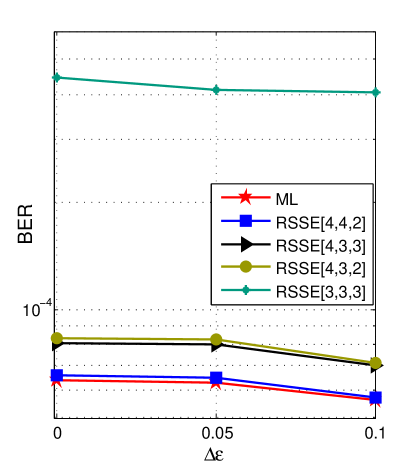
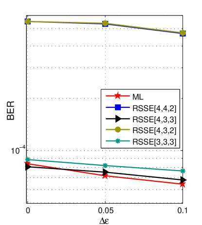
Refer to caption
(a) ϵ=0.1italic-ϵ0.1\epsilon=0.1
Refer to caption
(b) ϵ=0.4italic-ϵ0.4\epsilon=0.4
Figure 13: Performance of RSSE on asymmetric 2H2T EPR4 channel, at different ITI levels and various offsets.

We search for dmin2(Er)subscriptsuperscript𝑑2minsuperscript𝐸𝑟d^{2}_{\text{min}}(E^{r}) at ITI levels with two extreme values of ϵitalic-ϵ\epsilon and various offsets ΔϵΔitalic-ϵ\Delta\epsilon on the EPR4 channel. The results are listed in Table VII and Table VIII. In each case, ΔϵΔitalic-ϵ\Delta\epsilon could take values from {0,0.05,0.1}00.050.1\{0,0.05,0.1\}. For comparison, we also give the minimum distance parameter of the ML detector, denoted as dmin2subscriptsuperscript𝑑2mind^{2}_{\text{min}}, in each corresponding scenario. We find that dmin2(Er)subscriptsuperscript𝑑2minsuperscript𝐸𝑟d^{2}_{\text{min}}(E^{r}) does not change much from the symmetric case (Δϵ=0Δitalic-ϵ0\Delta\epsilon=0). In addition, some trellis configurations tend to have increased dmin2(Er)subscriptsuperscript𝑑2minsuperscript𝐸𝑟d^{2}_{\text{min}}(E^{r}) under severe asymmetry, while some do not. We see that the performance of a configuration is closely related to the distance parameters of the length-1 error events, which provides an approach to design the set partition tree for other MHMT channel models. The conclusion is that the proposed RSSE algorithm is applicable to the asymmetric channel. An example of BER vs. ΔϵΔitalic-ϵ\Delta\epsilon simulation result is shown in Figs. 13.

VI Conclusion

In this paper we deal with the problem of the high computational complexity of MHMT detection. The proposed RSSE algorithm with a modified set partition tree significantly reduces the number of trellis states while retaining near optimal performance. Performance was evaluated on both symmetric and asymmetric 2H2T channel models. Error event analysis was used to explain the performance variation for different trellises under different ITI conditions. If a suitable set partition tree is designed, the RSSE algorithm has the potential to be applied to more general MHMT channels. This is a direction for future research.

Acknowledgment

This work was supported in part by the National Science Foundation under Grant CCF-1405119, and the Center for Memory and Recording Research (formerly, Center for Magnetic Recording Research) at UC San Diego.

References

  • [1] R. Wood, M. Williams, A. Kavcic, and J. Miles, “The feasibility of magnetic recording at 10 terabits per square inch on conventional media,” IEEE Trans. Magn., vol. 45, no. 2, pp. 917–923, Feb. 2009.
  • [2] S. Karakulak, P. Siegel, J. Wolf, and H. Bertram, “A new read channel model for patterned media storage,” IEEE Trans. Magn., vol. 44, no. 1, pp. 193–197, Jan. 2008.
  • [3] G. Mathew, E. Hwang, J. Park, G. Garfunkel, and D. Hu, “Capacity advantage of array-reader-based magnetic recording (ARMR) for next generation hard disk drives,” IEEE Trans. Magn., vol. 50, no. 3, pp. 155–161, Mar. 2014.
  • [4] H. Xia, L. Lu, S. Jeong, L. Pan, and J. Xiao, “Signal processing and detection for array reader magnetic recording system,” in 2015 IEEE Int. Magn. Conf. (INTERMAG), Beijing, China, May 2015, pp. 1–1.
  • [5] E. Soljanin and C. Georghiades, “Multihead detection for multitrack recording channels,” IEEE Trans. Inf. Theory, vol. 44, no. 7, pp. 2988–2997, Nov. 1998.
  • [6] X. Ma and L. Ping, “Iterative detection/decoding for two-track partial response channels,” IEEE Commun. Lett., vol. 8, no. 7, pp. 464–466, Jul. 2004.
  • [7] L. Barbosa, “Simultaneous detection of readback signals from interfering magnetic recording tracks using array heads,” IEEE Trans. Magn., vol. 26, no. 5, pp. 2163–2165, Sep. 1990.
  • [8] M. Eyuboglu and S. Qureshi, “Reduced-state sequence estimation with set partitioning and decision feedback,” IEEE Trans. Commun., vol. 36, pp. 13–20, Jan. 1988.
  • [9] E. Kurtas, J. Proakis, and M. Salehi, “Reduced complexity maximum likelihood sequence estimation for multitrack high-density magnetic recording channels,” IEEE Trans. Magn., vol. 35, no. 4, pp. 2187–2193, Jul. 1999.
  • [10] B. Fan, H. Thapar, and P. Siegel, “Multihead multitrack detection with reduced-state sequence estimation in shingled magnetic recording,” in 2015 IEEE Int. Magn. Conf. (INTERMAG), Beijing, China, May 2015, pp. 1–1.
  • [11] W.-H. Sheen and G. L. Stuber, “Error probability for reduced-state sequence estimation,” IEEE J. Sel. Areas Commun., vol. 10, no. 3, pp. 571–578, Apr. 1992.
  • [12] G. Ungerboeck, “Channel coding with multilevel/phase signals,” IEEE Trans. Inf. Theory, vol. 28, no. 1, pp. 55–67, Jan. 1982.
  • [13] B. Fan, H. Thapar, and P. Siegel, “Multihead multitrack detection in shingled magnetic recording with iti estimation,” in 2015 IEEE Int. Conf. on Commun. (ICC), London, UK, Jun. 2015, pp. 425–430.
  • [14] G. D. Forney, “Maximum-likelihood sequence estimation of digital sequences in the presence of intersymbol interference,” IEEE Trans. Inf. Theory, vol. 18, no. 3, pp. 363–378, May 1972.
  • [15] S. A. Altekar, M. Berggren, B. E. Moision, P. H. Siegel, J. K. Wolf, and J. K. W. Fellow, “Error-event characterization on partial-response channels,” IEEE Trans. Inform. Theory, vol. 45, no. 1, pp. 241–247, Jan. 1998.