Hadron energy spectrum in polarized top quark decays considering the effects of hadron and bottom quark masses

Abstract

We present the analytical expressions for the next-to-leading order corrections to the partial decay width $t(\uparrow)\rightarrow bW^{+}$, followed by $b\rightarrow H_{b}X$, for nonzero b-quark mass ($m_{b}\neq 0$) in the fixed-flavor-number scheme (FFNs). To make the predictions for the energy distribution of outgoing hadrons $H_{b}$, as a function of the normalized $H_{b}$-energy fraction $x_{H}$, we apply the general-mass variable-flavor-number scheme (GM-VFNs) in a specific helicity coordinate system where the polarization of top quark is evaluated relative to the b-quark momentum. We also study the effects of gluon fragmentation and finite hadron mass on the hadron energy spectrum so that hadron masses are responsible for the low-$x_{H}$ threshold. In order to describe both the b-quark and the gluon hadronizations in top decays we apply realistic and nonperturbative fragmentation functions extracted through a global fit to $e^{+}e^{-}$ annihilation data from CERN LEP1 and SLAC SLC by relying on their universality and scaling violations.

I Introduction

Ever since the top quark discovery in $p\bar{p}$ collisions in 1995 by the CDF Abe:1995hr and D0 experiments Abachi:1995iq at the Fermilab Tevatron, it has been in or near the center of attention in high-energy physics. Its characteristics such as its mass $m_{t}$, total decay width $\Gamma_{t}$, branching fractions, and elements $V_{tq}$ of the Cabibbo-Kobayashi-Maskawa (CKM) quark mixing matrix, have not yet been determined precisely. Its property which is likely most central in many aspects of top physics is its mass. Since, for example, the top interacts with the Higgs boson through the potential $y_{t}h\bar{t}t$ where $y_{t}$ is proportional to the top mass $m_{t}$, therefore the top mass has a fundamental role in the issue of stability of the Higgs potential (see Eq. (5)). Using the full sample of $p\bar{p}$ collision data collected by the $D0$ experiment in the Tevatron Run II Abazov:2014dpa at a center-of-mass energy of $1.96$ TeV and for an integrated luminosity of up to $8.7$ $fb^{-1}$ the mass of top quark is measured as $m_{t}=174.98\pm 0.76$ GeV. Due to its remarkably large mass, the top couples strongly to the agents of electroweak symmetry breaking and this makes it both an object of interest itself, and a tool to investigate that mechanism in detail.
Among other things, the CERN LHC is a genuine top factory, in particular in Run II, producing about 90 million top quark pairs per year of running at design energy $14$ TeV. The existing and upcoming data will allow us to study the top quark and its behavior in LHC collisions in great detail, if also the theoretical descriptions and simulations are of proportionate quality.
The top decay width itself is very difficult to determine in hadron colliders, though a recent experimental inference of the width was performed by D0 Abazov:2012vd and found $\Gamma_{t}=2.00\pm 0.47$ GeV in the context of single top t-channel production, and CDF Aaltonen:2013kna also reported $1.10<\Gamma_{t}<4.05$ GeV at the $68\%$ confidence level. The top decay characteristics play an important role in studying the top quark at colliders. Since, the width-to-mass ratio $\Gamma_{t}/m_{t}$ of the top quark is small enough then, for many purpose, the notion of top quark as a stable particle makes sense, so that its production and decay processes can be factorized through the narrow width approximation delDuca:2015gca . In fact, if it were not for the confinement of color, the top could be considered as a free particle. This property allows it to behave like a real particle and one can safely describe its decay in perturbative theory.
The top decay width is largely due to decays to a W-boson and a bottom quark (with the mass $m_{b}$), as it is represented in the element $|V_{tb}|\approx 1$ of the CKM matrix Cabibbo:1963yz . Since $m_{t}>>m_{W}+m_{b}$, its width is sufficiently large to pre-empt top quark hadronization, then this rapid decay ($\tau_{t}\approx 0.5\times 10^{-24}$ s Chetyrkin:1999ju ) enables transmission of top quark spin information to final states. Part of the top attractiveness is its power to self-analyze its spin, through its purely left-handed Standard Model (SM) weak decay. The interplay between the top spin and its mass is of crucial importance in studying the SM. The top quark polarization can be studied by the angular correlations between the top quark spin and its decay product momenta, and these spin-momentum correlations will allow the detailed studies of the top decay mechanism. In Nejad:2013fba , we showed that these correlations depend on the choice of the possible helicity coordinate systems.
Since, produced b-quarks hadronize before they decay, then each $b$-jet contains a bottom flavored hadron which, most of the times, is a B-meson. They are identified by a displaced decay vertex associated which charged lepton tracks. In Corcella ; Corcella:2001hz , it is identified that the hadronization of the b-quark is the largest source of uncertainty in the measurement of the top mass at the LHC and the Tevatron. These nonperturbative transitions are described by realistic, nonperturbative fragmentation functions (FFs) that are usually obtained through a global fit to $e^{+}e^{-}$ data. At LHC, the decay process $t\rightarrow BW^{+}+X$ is of prime importance, and it is an urgent task to predict its partial decay width as reliably as possible, specifically the distribution in the scaled-energy of B-mesons ($x_{B}$) in the top quark rest frame is of particular interest. These $x_{B}$-distributions provide direct access to the B-meson FFs. In Nejad:2013fba , using the zero-mass variable-flavor-number scheme (ZM-VFNs) in which the mass of b-quarks are set to zero at the parton-level, we studied the NLO angular distribution of the scaled-energy of B-hadrons through polarized top decays. For that, we calculated the polar angular correlation in the rest frame decay of a polarized top quark into a stable $W^{+}$-boson and the B-hadron, i.e. $t(\uparrow)\rightarrow W^{+}+b(\rightarrow B+X)$. We analysed this correlation in a helicity coordinate system where the event plane, including the top quark and its decay products, is defined in the $(x,z)$-plane with the Z-axes along the b-quark momentum. Here, the top polarization vector was evaluated with respect to the b-momentum direction.
Here, using the same frame, we revisit B-hadron production from polarized top decays by working at NLO in the general-mass variable-flavor-number scheme (GM-VFNs), where b-quark masses are preserved from the beginning. This makes the calculations more complicated. Being manifestly based on Collin’s QCD factorization theorem Collins:1998rz convenient for massive quarks, this factorization scheme allows us to resum the large logarithms in $m_{b}$, to retain the finite-$m_{b}$ effects and to preserve the universality of the FFs, whose scaling violations remain to be subject to DGLAP evolution dglap . In this way, it combines the virtues of the fixed-flavor-number scheme (FFNs) and the ZM-VFN scheme and also avoids their flaws. In fact, it is an elaborat tool for global analyses of experimental data on the inclusive production of heavy flavored hadrons, allowing one to transfer nonperturbative information on the hadronization of partons from one type of experiment to another and from one energy scale $\mu_{F}$ to another, without the restriction $\mu_{F}>>m_{b}$ which is essential for the ZM-VFNs. Our analysis is supposed to enhance our previous result Nejad:2013fba in the ZM-VFN scheme by retaining all nonlogarithmic $m_{b}$-terms.
Moreover, we also include finite-$m_{B}$ effects, which modify the relations between hadronic and partonic scaling variables and reduce the available phase space. However, due to the smallness $m_{B}/m_{t}$, we do not expect to measure these additional effects truly, except for certain corners the phase space. Their study is nevertheless necessary to fully exploit the enormous statistics of the LHC data to be taken in the long run for a high precision determination of the top properties. Studying top decays could be important to deepen our conception of the nonperturbative aspects of B-mesons formation and to test the universality and scaling violations of the B-meson FFs.

II Top quark in the Standard Model

At first, we briefly review the various interactions of the top quark field $t(x^{\mu})$ in the SM Lagrangian; a topic needed for the calculation of top decay widths.
The charged weak interaction of the top quark is left-handed and flavor-changing, so expressed as

$$\frac{g_{w}}{2\sqrt{2}}V_{tf}\bar{t}(x)\gamma^{\mu}(1-\gamma_{5})f(x)W_{\mu}(x),$$ (1)

where $f(x)$ stands for the fields of down, strange and bottom quarks and the weak coupling factor $g_{w}$ is related to the Fermi coupling constant as $g_{w}^{2}=4\sqrt{2}m_{W}^{2}G_{F}$, while its neutral weak interaction is flavor-conserving and parity violating

$$\frac{g_{w}}{4\cos\theta_{w}}\bar{t}(x)\gamma^{\mu}[(1-\frac{8}{3}\sin^{2}\theta_{w})-\gamma_{5}]t(x)Z_{\mu}(x),$$ (2)

where $\theta_{w}$ is the weak mixing angle, so that $\sin^{2}\theta_{w}=0.23124$ Caso:1998tx . Its interaction with gluons is a vector-like coupling, involving an SU(3) generator ($T^{a}$) in the fundamental representation

$$g_{s}\bar{t}_{i}(x)\gamma^{\mu}T_{ij}^{a}t_{j}(x)G_{\mu}^{a}(x),$$ (3)

where $g_{s}$ is the strong coupling constant, $a=1,2,\cdots 8$ is the QCD color index so $Tr(T^{a}T^{a})/3=C_{F}$. The top interaction with photons is also simply vector-like as

$$\frac{2}{3}e[\bar{t}(x)\gamma^{\mu}t(x)A_{\mu}(x)],$$ (4)

that is proportional to the top quark electric charge.
Finally, the interaction of the top quark with the Higgs field $h(x)$ is of the Yukawa type

$$y_{t}h(x)\bar{t}(x)t(x),$$ (5)

with a coupling constant $y_{t}=\sqrt{2}m_{t}/v$, where $v$ is the Higgs vacuum expectation value. The Yukawa coupling is almost $y_{t}\approx 1$ in the SM.
In many extensions of the SM such as minimal supersymmetric standard model (MSSM), the Higgs sector of the SM is enlarged by considering an extra doublet of complex Higgs field Li:1990cp ; Gunion:1984yn ; Gunion . In MoosaviNejad:2011yp , we studied the top decay in the general two Higgs doublet model (2HDM).
Moreover, beyond the interactions above, effective interactions such as for flavor-changing neutral currents occur due to loop corrections. However, they are generally very small in comparison with those above. All these interactions could be modified in structure and strength by virtual effects due to new interactions associated with the physics beyond the SM. This is of interest to investigate that if the top quark, evidently, has a large coupling to the electroweak symmetry breaking sector. Therefore, it is so important to test these structures in detail, and indeed this is the thrust behind the field of top physics.
One proposed way to study the properties of top quarks is to consider the scaled-energy distribution of outgoing hadrons. In next section we shall study this approach in detail, using the GM-VFN scheme where the mass of b-quark is preserved from the beginning.

III Formalism

We consider the decay process of polarized on-shell top quark at NLO, as

$$t(\uparrow)\rightarrow b+W^{+}(+g)\rightarrow B+X,$$ (6)

where, $X$ stands for the unobserved final-state particles. We wish to study the angular distribution of the scaled-energy of B-hadrons by considering the contribution of bottom and gluon fragmentations into the heavy meson B, so that the gluon contributes to the real radiation at NLO. To obtain this energy spectrum, we need to have the parton-level differential width of the process (6). The LO contribution results from $t(\uparrow)\rightarrow bW^{+}$. We define the partonic scaled-energy fraction $\textbf{x}_{i}=2p_{i}\cdot p_{t}/m_{t}^{2}$, where $p_{i}$ stands for the gluon or bottom quark momenta. In the top quark rest frame where $p_{t}=(m_{t},\vec{0})$, one has $\textbf{x}_{i}=2E_{i}/m_{t}$ where $E_{i}$ refers to the energy of outgoing partons; gluon or bottom at NLO. By preserving the bottom quark mass, one has $\textbf{x}_{b}^{max}=1+b-\omega$ in which $b=m_{b}^{2}/m_{t}^{2}$ and $\omega=m_{W}^{2}/m_{t}^{2}$. As in Corcella:2001hz , throughout this paper, we shall make use of the normalized energy fraction of partons as

$$x_{i}=\frac{\textbf{x}_{i}}{\textbf{x}_{b}^{max}}=\frac{2E_{i}}{m_{t}(1+b-\omega)},\quad(i=b,g).$$ (7)

The allowed values of $x_{b}$ and $x_{g}$ shall be discussed in Section V. We analyse the decay $t(\uparrow)\rightarrow bW^{+}$ in the rest frame of the top quark where the 3-momentum of the b-quark points to the direction of the positive Z-axis. For a polarized top quark, the general angular distribution of differential decay width $d\Gamma/dx$ is given by

$$\frac{d^{2}\tilde{\Gamma}}{dx_{i}d\cos\theta_{P}}=\frac{1}{2}\bigg{(}\frac{d\tilde{\Gamma}^{unpol}}{dx_{i}}+P\frac{d\tilde{\Gamma}^{pol}}{dx_{i}}\cos\theta_{P}\bigg{)}.$$ (8)

This form clarifies the correlations between the top decay products and the spin of the top quark.
In (8), $P$ is the magnitude of the top-quark polarization with $0\leq P\leq 1$, so that $P=0$ corresponds to an unpolarized top quark and $P=1$ is for the $100\%$ polarization. Here, $\theta_{P}$ is defined as the polar angle between the top quark polarization vector $\vec{P}$ and the Z-axis (b-quark momentum direction).
In (8), $d\tilde{\Gamma}^{unpol}/dx_{i}$ refers to the unpolarized differential widths which studied in Kniehl:2012mn , both in ZM- and GM-VFN schemes. In following, we discuss the evaluation of the quantities $d\tilde{\Gamma}^{pol}/dx_{i}$ in the GM-VFN scheme.

IV Parton-level results in the SM

IV.1 Born term result

Considering the charged weak interaction Lagrangian (1), the dynamics of the current-induced $t\rightarrow b$ transition is presented in the tensor $H^{\mu\nu}\propto\left\langle t\right|J^{\nu{\dagger}}\left|X_{b}\right\rangle\left\langle X_{b}\right|J^{\mu}\left|t\right\rangle$ in which the weak current is $J^{\mu}\propto V_{tb}\bar{t}(x)\gamma^{\mu}(1-\gamma_{5})b(x)$, and at the Born level and ${\cal O}(\alpha_{s})$ one-loop contributions the intermediate state is $\left|X_{b}\right\rangle=\left|b\right\rangle$. Also, this hadronic tensor depends on the top spin $s_{t}$. It is straightforward to compute the Born term contribution to the decay (6). In the top rest frame, the four-momentum of the bottom quark is set to $p_{b}=(E_{b};0,0,p_{b})$ and the polarization four-vector of the top quark is set as $s_{t}=P(0;\sin\theta_{P}\cos\phi_{P},\sin\theta_{P}\sin\phi_{P},\cos\theta_{P})$. Considering the general distribution (8), the Born term helicity structure of partial rates, reads

$$\frac{d\tilde{\Gamma}^{\textbf{(0)}}}{d\cos\theta_{P}} = \frac{1}{2}\bigg{\{}\tilde{\Gamma}_{A}^{\textbf{(0)}}-P\tilde{\Gamma}_{B}^{\textbf{(0)}}\cos\theta_{P}\bigg{\}},$$ (9)

where, the LO polarized ($\tilde{\Gamma}_{B}^{\textbf{(0)}}$) and unpolarized ($\tilde{\Gamma}_{A}^{\textbf{(0)}}$) total decay widths read

$$\tilde{\Gamma}_{A}^{\textbf{(0)}} = \frac{m_{t}\alpha Q}{4\sin^{2}\theta_{W}}G_{0},$$

$$\tilde{\Gamma}_{B}^{\textbf{(0)}} = \frac{m_{t}\alpha Q^{2}}{4\sin^{2}\theta_{W}}\frac{1-b-2\omega}{\omega}.$$ (10)

Here, we used the following kinematic variables, in the notations of Ref. Corcella:2001hz

$$S=\frac{1}{2}(1+b-\omega),\quad\beta=\frac{\sqrt{b}}{S},\quad Q=S\sqrt{1-\beta^{2}},$$

$$G_{0}=\frac{1}{2}(1+b-2\omega+\frac{(1-b)^{2}}{\omega}).$$ (11)

In the limit of vanishing bottom quark mass, the tree-level decay widths converted to our results in Nejad:2013fba and Kniehl:2012mn , respectively.

IV.2 Virtual corrections and counterterms

The QCD one-loop vertex corrections arise from the emission and absorption of the virtual gluons, so an interaction Lagrangian as in (3) is needed to calculate the virtual radiative corrections. Here, we adopt the on-shell mass renormalization scheme and use dimensional regularization to regulate the ultraviolate (UV) and soft singularities which appear in one-loop corrections. For example, the UV-singularities appear when the integration region of the internal momentum of the virtual gluon goes to infinity. The singularities are regularized by dimensional regularization in $D=4-2\epsilon$ space-time dimensions to become single poles in $\epsilon$, so that $0<\epsilon\leq 1$. In the massless case, all singularities are subtracted at factorization scale $\mu_{F}$ and absorbed into the bare FFs in accordance with the modified minimal subtraction ($\overline{MS}$) scheme, see Nejad:2013fba . In the massive case, all singularities are automatically canceled after summing all radiative corrections up.
Considering the notations (IV.1), the contribution of virtual corrections into the doubly differential decay width (8) is obtained as

$$\frac{d^{2}\tilde{\Gamma}^{vir}}{dx_{b}d\cos\theta_{P}}=\frac{Q}{16\pi m_{t}}\bigg{\{}2Re(M_{0}^{\dagger}M_{\rm 1-loop})\bigg{\}}\delta(1-x_{b}),$$ (12)

where $M_{0}$ stands for the Born term amplitude and the renormalized amplitude $M_{\rm 1-loop}$ refers to the virtual gluon corrections, presented in Nejad:2013fba . The virtual contributions include the counterterm and the one-loop vertex corrections. The counterterm of the vertex contains the wave-function renormalization constants of the top ($\delta Z_{t}$) and the bottom quark ($\delta Z_{b}$). These constants can be found in Nejad:2013fba .
The wave-function renormalization and the one-loop vertex correction contain the UV and infrared (IR) singularities so that all UV-divergences are canceled after summing all virtual corrections up and, from now on, we label the remaining IR-singularities by $\epsilon$. Therefore, the virtual decay width is given by

$$\frac{d^{2}\tilde{\Gamma}^{vir}}{dx_{b}d\cos\theta_{P}}=\frac{1}{2}\Big{(}\frac{d\tilde{\Gamma}_{A}^{vir}}{dx_{b}}+P\frac{d\tilde{\Gamma}_{B}^{vir}}{dx_{b}}\cos\theta_{P}\Big{)}\delta(1-x_{b}),$$ (13)

where the unpolarized differential decay rate reads

$$\frac{d\tilde{\Gamma}_{A}^{vir}}{dx_{b}}=\tilde{\Gamma}_{A}^{(0)}\frac{C_{F}\alpha_{s}}{2\pi}\Big{\{}\tilde{H}+\frac{6Q}{G_{0}}\ln\frac{S+Q}{\sqrt{b}}+\frac{3S(b-1)}{2\omega G_{0}}\ln b\Big{\}},$$ (14)

and the polarized one is expressed by

$$\frac{d\tilde{\Gamma}_{B}^{vir}}{dx_{b}}=\tilde{\Gamma}_{B}^{(0)}\frac{C_{F}\alpha_{s}}{2\pi}\Big{\{}\tilde{H}+\frac{3b-1}{2(1+3b-4S)}\ln b+\frac{2(1+3S)\omega-2(1-b)}{Q(1+3b-4S)}\ln\frac{S+Q}{\sqrt{b}}\Big{\}},$$ (15)

where,

$$\tilde{H}=2F\Big{(}-1+\frac{S}{Q}\ln\frac{S+Q}{\sqrt{b}}\Big{)}-2\frac{Q+2S}{S}+\frac{2S}{Q}\ln(S+Q)\ln\frac{1-S-Q}{1-S+Q}-\ln b+\frac{2S}{Q}\Big{(}Li_{2}\frac{2Q}{1+Q-S}-Li_{2}\frac{2Q}{S+Q-b}\Big{)}.$$

In the equations above, $C_{F}=(N_{c}^{2}-1)/(2N_{c})=4/3$ is the color factor, $\gamma_{E}$ is the Euler constant, $Li_{2}(x)$ is the dilogarithmic function (or Spence function) and the term $F$ includes the IR-singularity ($\epsilon$) as

$$F=\frac{1}{\epsilon}-\frac{Q}{S}-\gamma_{E}+\ln\frac{4\pi\mu_{F}^{2}}{m_{t}^{2}}-\ln\frac{S+Q}{\sqrt{b}}-\ln b.$$ (17)

Here, $\mu_{F}$ stands for the factorization scale which will be removed after summing all corrections up in the GM-VFN scheme.

IV.3 Real gluon corrections

The ${\cal O}(\alpha_{s})$ real graph contributions result from the real gluon emissions from the bottom and top quarks, individually. In the rest frame of a top quark decaying into a b-quark, a $W^{+}$ boson and a gluon, the outgoing particles define an event plane. Relative to this plane one can, then, define the spin direction of the polarized top quark. As in Nejad:2013fba , here we apply a specific helicity coordinate system where the momenta of the b-quark and the $W^{+}$ boson are defined as; $\vec{p}_{b}||\hat{z},(\vec{p}_{W})_{x}\geq 0$, and the polarization vector of top quark is evaluated relative to the $\hat{z}$-axis. In the following, we explain a brief technical detail of our calculation for the NLO radiative corrections to the tree-level decay rate of $t(\uparrow)\rightarrow bW$.

In Nejad:2013fba , where we set the mass of b-quark to zero from the first, the IR-singularities arised from the soft- and collinear gluon emissions. Since, here, we preserve the mass of b-quark then all IR-singularities arise from the soft real-gluon emission and the collinear divergences would be absent. As before, to regularize the IR-singularities we work in D-dimensions where the real differential rate is given by

$$d\tilde{\Gamma}^{real}=\frac{\mu_{F}^{2(4-D)}}{2m_{t}}\left|M^{real}\right|^{2}\prod_{i=b,g,W}\frac{d^{D-1}\vec{p_{i}}}{(2\pi)^{D-1}2E_{i}}(2\pi)^{D}\delta^{D}(p_{t}-\sum_{i=b,g,W}p_{i}).$$ (18)

To compute the differential rate $d\tilde{\Gamma}^{real}/dx_{b}$, we fix the b-quark momentum and integrate over the gluon energy which ranges from $E_{g}^{max}=m_{t}S(1-x_{b})/(1-Sx_{b}+S\sqrt{x_{b}^{2}-\beta^{2}})$ to $E_{g}^{min}=m_{t}S(1-x_{b})/(1-Sx_{b}-S\sqrt{x_{b}^{2}-\beta^{2}})$. In the GM-VFN scheme the real and virtual differential widths include the pole $\propto 1/\epsilon$, which shall disappear in the total NLO result. Due to the radiation of a soft gluon ($E_{g}\rightarrow 0$) in top decay, during integration over the phase space for the real gluon radiation, terms of the form $(1-x_{b})^{-1-2\epsilon}$ arise which are divergent when $x_{b}\rightarrow 1$. Therefore, for a massive scheme ($m_{b}\neq 0$) where $\beta\leq x_{b}\leq 1$, we shall make use of the following expression Corcella:2001hz

$$\frac{(1-x_{b})^{-1-2\epsilon}}{(x_{b}-\beta)^{-2\epsilon}}=-\frac{1}{2\epsilon}\delta(1-x_{b})+\frac{1}{(1-x_{b})_{+}}+{\cal O}(\epsilon),$$ (19)

with the plus prescription defined as

$$\int_{\beta}^{1}[g(x_{b})]_{{}_{+}}h(x_{b})dx_{b}=\int_{\beta}^{1}g(x_{b})[h(x_{b})-h(1)]dx_{b}.$$ (20)

IV.4 Parton-level results for angular distribution of partial decay rates in FFN scheme

Considering the tree-level, the real and virtual contributions, we present our analytic expression for the angular distribution of the partial decay rate in the FFN scheme. According to the Lee-Nauenberg theorem, after summing all corrections up the singularities cancel each other and the final result is free of IR-singularities. Therefore, the complete NLO results read

$$\frac{d^{2}\tilde{\Gamma}}{dx_{b}d\cos\theta_{P}}=\frac{1}{2}\Big{(}\frac{d\tilde{\Gamma}_{NLO}^{unpol}}{dx_{b}}+P\frac{d\tilde{\Gamma}_{NLO}^{pol}}{dx_{b}}\cos\theta_{P}\Big{)},$$ (21)

where $d\tilde{\Gamma}_{NLO}^{unpol}/dx_{b}$ is given in Corcella:2001hz ; Kniehl:2012mn , and $d\tilde{\Gamma}_{NLO}^{pol}/dx_{b}$ in the $\overline{MS}$ scheme is presented, for the first time, as

$$\frac{1}{\tilde{\Gamma}_{B}^{(0)}}\frac{d\tilde{\Gamma}_{NLO}^{pol}}{dx_{b}}= \delta(1-x_{b})+\frac{C_{F}\alpha_{s}}{2\pi}\Big{\{}\delta(1-x_{b})\bigg{[}-4-\frac{1-8S+9b}{2(1-b-2\omega)}\ln b+\frac{1}{Q}\ln\frac{1+Q-S}{1-S-Q}\bigg{(}1-b-2S\ln(S+Q)\bigg{)}+$$ (22)

$$4\ln\frac{\sqrt{\omega}}{2S(1-\beta)}+\frac{4S}{Q}Li_{2}\frac{2Q}{1+Q-S}-\frac{4S}{Q}Li_{2}\frac{2Q}{S+Q-b}+\frac{2S}{Q}\ln\frac{S+Q}{\sqrt{b}}\bigg{(}2\ln\frac{2S}{1+Q-S}-2\ln\frac{S+Q}{1-\beta}+$$

$$1-\frac{b}{S}+\frac{1-b-\omega(1+3S)}{S(1-b-2\omega)}\bigg{)}\bigg{]}+\frac{2(1-x_{b})}{Q^{2}(1-b-2\omega)}\bigg{[}4S^{3}(x_{b}^{2}-2)+\frac{2S\omega}{\sqrt{x_{b}^{2}-\beta^{2}}}\ln\phi_{2}(x_{b})+2\frac{(1-b)S^{2}\omega}{1+b-2Sx_{b}}$$

$$+bS(4-3Sx_{b})+4S-S^{2}(5+x_{b}-5b)+\frac{\phi_{3}(x_{b})}{\sqrt{x_{b}^{2}-\beta^{2}}}\bigg{(}Sx_{b}(b+2\omega-1)-4(\omega+S^{2}x_{b}^{2})\bigg{)}\bigg{]}+$$

$$\frac{2}{Q^{2}(1-x_{b})_{+}}\bigg{[}x_{b}S^{2}-b-\frac{2x_{b}S^{3}(1-x_{b})^{2}}{1-b-2\omega}\bigg{]}\bigg{[}x_{b}-2-\frac{x_{b}}{2\sqrt{x_{b}^{2}-\beta^{2}}}\bigg{(}\ln b+2\frac{\phi_{3}(x_{b})}{S}-2\ln\phi_{1}(x_{b})\bigg{)}\bigg{]}\Big{\}},$$

where

$$\phi_{1}(x_{b}) = \frac{S(x_{b}+\sqrt{x_{b}^{2}-\beta^{2}})-b}{1-S(x_{b}-\sqrt{x_{b}^{2}-\beta^{2}})},$$

$$\phi_{2}(x_{b}) = \frac{S(x_{b}-\sqrt{x_{b}^{2}-\beta^{2}})-b}{S(x_{b}+\sqrt{x_{b}^{2}-\beta^{2}})-b},$$

$$\phi_{3}(x_{b}) = S(\sqrt{x_{b}^{2}-\beta^{2}}-artanh\frac{\sqrt{x_{b}^{2}-\beta^{2}}}{x_{b}}).$$ (23)

Since the B-mesons can be also produced through the fragmentation of emitted real gluons, then to obtain the most accurate result for the energy spectrum of mesons one needs the doubly differential distribution $d^{2}\tilde{\Gamma}/(dx_{g}d\cos\theta_{P})$ where the scaled-variable $x_{g}$ is defined in (7). As we will show in Fig. 1, the contribution of the gluon fragmentation into the B-meson is negative and leads to a significant reduction in size in the threshold region, so that this contribution would be important at a low energy of the observed meson.
To get the $d^{2}\tilde{\Gamma}/(dx_{g}d\cos\theta_{P})$, one has to integrate over the b-quark energy by fixing the gluon momentum in the phase-space so that the b-quark energy ranges as $m_{t}S\phi_{-}(x_{g})\leq E_{b}\leq m_{t}S\phi_{+}(x_{g})$, where

$$\phi_{\pm}(x_{g})=\frac{1-x_{g}}{1-2Sx_{g}}\big{[}1-Sx_{g}\pm Sx_{g}\sqrt{1-\frac{(1-2Sx_{g})\beta^{2}}{(1-x_{g})^{2}}}\big{]}.$$ (24)

The $d\tilde{\Gamma}_{NLO}^{unpol}/dx_{g}$ in the FFN scheme is given in Kniehl:2012mn , and by considering the following notations

$$A_{1}= x_{g}S^{3}(1+(1-x_{g})^{2})+\frac{8S^{2}(1-S)(1-x_{g})}{3(1+3b-4S)}x_{g}-\frac{S^{2}}{3}(4x_{g}^{2}+2x_{g}+3)+S(\frac{x_{g}}{2}+\frac{2}{3})+\frac{1}{6}(1+3b-4S)(1-3Sx_{g})-\frac{1}{6},$$ (25)

$$A_{2}=\frac{S^{3}x_{g}(1-x_{g})^{3}}{[(1-x_{g})^{2}-\beta^{2}]^{\frac{3}{2}}}\Big{[}1+(1-x_{g})^{2}-\frac{4+3x_{g}(x_{g}-2)}{(1-x_{g})^{2}}\beta^{2}+\frac{2+x_{g}(Sx_{g}-2)}{(1-x_{g})^{3}}\beta^{4}\Big{]},$$

and $A_{3}=\frac{2}{3}S\bigg{(}3+Sx_{g}^{2}+(3S-4)x_{g}-8\frac{(1-S)(1-Sx_{g})}{1+3b-4S}x_{g}\bigg{)}$, the polarized contribution reads

$$\frac{1}{\tilde{\Gamma}_{B}^{(0)}}\frac{d\tilde{\Gamma}_{NLO}^{pol}}{dx_{g}} = \frac{C_{F}\alpha_{s}}{4\pi Q^{2}x_{g}^{2}}\Big{\{}2\frac{A_{1}}{S}\ln\frac{\phi_{+}+\sqrt{\phi_{+}^{2}-\beta^{2}}}{\phi_{-}+\sqrt{\phi_{-}^{2}-\beta^{2}}}+2\frac{A_{2}}{S}\bigg{[}\ln\frac{(1-2Sx_{g})(1-x_{g}-\phi_{+})^{2}}{bx_{g}^{2}}$$ (26)

$$+\ln\frac{\beta^{2}+(x_{g}-1)\phi_{-}-\sqrt{((1-x_{g})^{2}-\beta^{2})(\phi_{-}^{2}-\beta^{2})}}{\beta^{2}+(x_{g}-1)\phi_{+}-\sqrt{((1-x_{g})^{2}-\beta^{2})(\phi_{+}^{2}-\beta^{2})}}\bigg{]}+A_{3}(\sqrt{\phi_{+}^{2}-\beta^{2}}-\sqrt{\phi_{-}^{2}-\beta^{2}})$$

$$+\frac{2S(1-2Sx_{g})}{\beta^{2}-(1-x_{g})^{2}}(1-x_{g}-\beta^{2})\bigg{[}\sqrt{\phi_{-}^{2}-\beta^{2}}(x_{g}-1+\phi_{+})-\sqrt{\phi_{+}^{2}-\beta^{2}}(x_{g}-1+\phi_{-})\bigg{]}$$

$$+S(1-Sx_{g})\bigg{[}\phi_{-}\sqrt{\phi_{-}^{2}-\beta^{2}}-\phi_{+}\sqrt{\phi_{+}^{2}-\beta^{2}}\bigg{]}\Big{\}}.$$

IV.5 General-mass variable-flavor-number scheme

In Nejad:2013fba , for obtaining the parton-level results for angular distribution of partial decay rates we used the ZM-VFN scheme, where $m_{b}=0$ was put right from the beginning and all collinear singularities were absorbed into the bare FFs according to the $\overline{MS}$ scheme. This approach renormalizes the FFs and produces finite terms of the form $(\alpha_{s}/\pi)\ln(\mu_{F}^{2}/m_{t}^{2})$ in the partial decay rates $d\hat{\Gamma}/dx_{a}$, which are rendered perturbatively small by choosing $\mu_{F}={\cal O}(m_{t})$. In this scheme, the b-quark mass $m_{b}$ just sets the initial scale $\mu_{F}^{ini}={\cal O}(m_{b})$ of the DGLAP evolution equations, where ansaetze for the $z$-dependences of the FFs $D_{a}(z,\mu_{F}^{ini})$ are injected by some proposed models jm . The DGLAP evolution from $\mu_{F}^{ini}$ to a higher scale $\mu_{F}$ then effectively resums the problematic logarithms $(\alpha_{s}/\pi)\ln(m_{t}^{2}/m_{b}^{2})$ of the FFN scheme, however, all information on the $m_{b}$-dependence of $d\hat{\Gamma}/dx_{a}$ is wasted.

The GM-VFN scheme provides an ideal theoretical framework to study the effects of heavy quark masses, so it combines the virtues of the ZM-VFN and FFN schemes and, at the same time, avoids their flaws. In the GM-VFN scheme, the perturbative fragmentation functions enter the formalism via subtraction terms for the hard scattering decay rates, so that the actual FFs are truly nonperturbative and may be assumed to have some smooth forms which can be specified through global data fits. In opposition with the FFN scheme, the GM-VFN scheme also accommodates FFs for light quarks and gluons, as in the ZM-VFN scheme. In our present work, the GM-VFNs is applied to resum the large logarithms in $m_{b}$ and to retain the entire nonlogarithmic $m_{b}$-dependence at the same time. This is reached by introducing convenient subtraction terms in the ${\cal O}(\alpha_{s})$ FFN expressions for $d\tilde{\Gamma}/dx_{i}$, so that the ${\cal O}(\alpha_{s})$ ZM-VFN results are exactly recovered in the limit $m_{b}/m_{t}\rightarrow 0$. These subtraction terms are universal and so are the FFs in the FFN scheme, as is guaranteed by Collin’s hard-scattering factorization theorem Collins:1998rz .

As explained above, the GM-VFN results for the angular decay distributions are obtained by matching the FFN results (22,26) to the ZM-VFN ones Nejad:2013fba by subtraction, as

$$\frac{1}{\Gamma_{0}}\frac{d\Gamma}{dx_{i}}\Big{|}_{GM-VFN}=\frac{1}{\Gamma_{0}}\frac{d\tilde{\Gamma}}{dx_{i}}\Big{|}_{FFN}-\frac{1}{\Gamma_{0}}\frac{d\Gamma}{dx_{i}}\Big{|}_{Sub},$$ (27)

where the subtraction terms are obtained as

$$\frac{1}{\Gamma_{0}}\frac{d\Gamma}{dx_{i}}\Big{|}_{Sub}=\lim_{m_{b}\rightarrow 0}\frac{1}{\Gamma_{0}}\frac{d\tilde{\Gamma}}{dx_{i}}\Big{|}_{FFN}-\frac{1}{\Gamma_{0}}\frac{d\hat{\Gamma}}{dx_{i}}\Big{|}_{{}_{ZM-VFN}}.$$ (28)

Taking the limit $m_{b}\rightarrow 0$ in (22) and (26), we recover the results presented in Nejad:2013fba up to the terms

$$\frac{1}{\Gamma_{0}}\frac{d\Gamma}{dx_{b}}\Big{|}_{Sub}=\frac{\alpha_{s}(\mu_{R})}{2\pi}C_{F}\Big{\{}\frac{1+x_{b}^{2}}{1-x_{b}}\Big{[}\ln\frac{\mu_{F}^{2}}{m_{b}^{2}}-2\ln(1-x_{b})-1\Big{]}\Big{\}}_{+},$$ (29)

and,

$$\frac{1}{\Gamma_{0}}\frac{d\Gamma}{dx_{g}}\Big{|}_{Sub}=\frac{\alpha_{s}(\mu_{R})}{2\pi}C_{F}\frac{1+(1-x_{g})^{2}}{x_{g}}\Big{(}\ln\frac{\mu_{F}^{2}}{m_{b}^{2}}-2\ln x_{g}-1\Big{)}.$$ (30)

As we have already shown in Kniehl:2012mn , for the unpolarized top decay in the SM, i.e. $t\rightarrow bW^{+}$, and also for the top decay in the theories beyond the SM including the two Higgs doublet where $t\rightarrow bH^{+}$ MoosaviNejad:2011yp , Eq. (29) coincides with the perturbative FF of the transition $b\rightarrow b$. This is in agreement with the Collin’s factorization theorem which guarantees that the subtraction terms are universal. Thus the results presented in (29) and (30) ensure the correctness of our calculations shown in (22,26).

V Hadron mass effects and Hadron level results

Our main purpose is to obtain the scaled-energy ($x_{B}$) distribution of bottom-flavored hadrons (B) inclusively produced in polarized top decays at NLO. Here, the scaled-energy fraction of B-hadrons is defined as $x_{B}=2E_{B}/(m_{t}(1+b-\omega))$, as in (7). In Nejad:2013fba , to obtain the partial decay width of the process (6) in the ZM-VFN scheme, we used the Collin’s factorization theorem Collins:1998rz . According to this theorem, the energy distribution of B-hadrons might be expressed as the convolution of the partonic hard scattering decay rates $d\Gamma/dx_{a}$, with the nonperturbative FFs which describe the transition $a\rightarrow B$, as

$$\frac{d\Gamma}{dx_{B}}=\sum_{a=b,g}\int_{x_{a}^{min}}^{x_{a}^{max}}\frac{dx_{a}}{x_{a}}\frac{d\hat{\Gamma}}{dx_{a}}(\mu_{R},\mu_{F})D_{a}^{B}(\frac{x_{B}}{x_{a}},\mu_{F}).$$ (31)

Here, $\mu_{F}$ and $\mu_{R}$ are the factorization and the renormalization scales, respectively. The $\mu_{R}$ is associated with the renormalization of the strong coupling constant and a choice often applied is $\mu_{R}=\mu_{F}$.

In the massless (or ZM-VFN) scheme where one sets $m_{b}=0$, the b-quark, gluon and B-hadron (with the mass $m_{B}$) have energies $0\leq(E_{b},E_{g})\leq(m_{t}^{2}-m_{W}^{2})/(2m_{t})$ and $m_{B}\leq E_{B}\leq(m_{t}^{2}+m_{B}^{2}-m_{W}^{2})/(2m_{t})$, respectively.

As we demonstrated in Kniehl:2012mn , the relation (31) is convenient for the case $m_{b}=0=m_{B}$. To calculate the $d\Gamma/dx_{B}$ when passing from the ZM-VFN scheme to the GM-VFN scheme by taking into account the finite-$m_{B}$ corrections, one should apply the following improved relation

$$\frac{d\Gamma}{dx_{B}}=\frac{1}{\sqrt{x_{B}^{2}-\rho_{B}^{2}}}\sum_{a=b,g}\int_{x_{a}^{min}}^{x_{a}^{max}}dx_{a}z\frac{d\Gamma}{dx_{a}}\Big{|}_{{}_{GM-VFN}}D_{a}^{B}(z,\mu_{F}),$$ (32)

where $(d\Gamma/dx_{a})_{{}_{{}_{GM-VFN}}}$ is given in (27), and

$$z=\frac{x_{B}+\sqrt{x_{B}^{2}-\rho_{B}^{2}}}{x_{a}+\sqrt{x_{a}^{2}-\rho_{a}^{2}}},$$ (33)

with $\rho_{i}=m_{i}/E_{b}^{max}(i=b,g,B)$, so $E_{b}^{max}=(m_{t}^{2}+m_{b}^{2}-m_{W}^{2})/(2m_{t})$. Now, the kinematically allowed scaling-variables are

$$\frac{1}{2}(x_{B}+\sqrt{x_{B}^{2}-\rho_{B}^{2}}+\frac{\rho_{b}^{2}}{x_{B}+\sqrt{x_{B}^{2}-\rho_{B}^{2}}})\leq x_{b}\leq 1,$$

$$\frac{1}{2}(x_{B}+\sqrt{x_{B}^{2}-\rho_{B}^{2}})\leq x_{g}\leq\frac{m_{t}^{2}-(m_{b}+m_{W})^{2}}{m_{t}^{2}+m_{b}^{2}-m_{W}^{2}},$$

$$\rho_{B}\leq x_{B}\leq\frac{m_{t}^{2}+m_{B}^{2}-m_{W}^{2}}{m_{t}^{2}+m_{b}^{2}-m_{W}^{2}}\quad\textrm{for b-quark transition},$$

$$\rho_{B}\leq x_{B}\leq\frac{m_{t}^{2}+m_{B}^{2}-(m_{b}+m_{W})^{2}}{m_{t}^{2}+m_{b}^{2}-m_{W}^{2}}\quad\textrm{for gluon transition}.$$ (34)

Clearly, if $m_{b}=0$ and $m_{B}=0$ are put ($z\rightarrow x_{B}/x_{a}$), then (31) and (32) coincide by reproducing the familiar factorization formula of the massless parton model.

VI Numerical analysis

By having the necessary tools, we now turn our attention to the phenomenological predictions of the B-hadron energy spectrum in polarized top decays, considering the effects of bottom quark and B-hadron masses. From Nakamura:2010zzi , we adopt the input parameter values $m_{W}=80.399$ GeV, $m_{t}=172.98$ GeV,$m_{b}=4.78$ GeV, $m_{B}=5.279$ GeV, $\sin^{2}\theta_{W}=0.2312$ and we evaluate $\alpha_{s}^{(n_{f})}(\mu_{R})$ at NLO in the $\overline{MS}$ scheme, using

$$\alpha_{s}^{(n_{f})}(\mu_{R})=\frac{1}{b_{0}\log[\mu_{R}^{2}/(\Lambda^{(n_{f})})^{2}]}\bigg{\{}1-\frac{b_{1}\log(\log[\mu_{R}^{2}/(\Lambda^{(n_{f})})^{2}])}{b_{0}^{2}\log[\mu_{R}^{2}/(\Lambda^{(n_{f})})^{2}]}\bigg{\}},$$ (35)

where, $n_{f}$ is the number of active quark flavors and

$$b_{0}=\frac{33-2n_{f}}{12\pi},\quad b_{1}=\frac{153-19n_{f}}{24\pi^{2}}.$$ (36)

Considering $n_{f}=5$, we adopt the asymptotic scale parameter $\Lambda_{\overline{MS}}^{(5)}=231$ MeV, adjusted such that $\alpha_{s}^{(5)}(m_{Z})=0.1184$ for $m_{Z}=91.1876$ GeV Nakamura:2010zzi . To include the B-meson and the b-quark masses, we apply Eq. (32) in which for the transitions $(b,g)\rightarrow B$, from Kniehl:2008zza we employ the related realistic and nonperturbative FFs. In Kniehl:2008zza , a power model as $D_{b}^{B}(z,\mu_{0})=Nz^{\alpha}(1-z)^{\beta}$ is used for the transition $b\rightarrow B$ at the initial scale $\mu_{F}=4.5$ GeV of fragmentation, while the FFs of gluon and light quarks are set to zero at the starting scale and are evolved to higher scales via the DGLAP equations dglap . The fit parameters are obtained at NLO in the ZM-VFN scheme through a global fit to $e^{+}e^{-}$ annihilation data from the ALEPH and OPAL collaborations at CERN LEP1 and by SLD at SLAC SLC and the results are $N=4684.1,\alpha=16.87$ and $\beta=2.628$.
In Fig. 1, our predictions for the scaled-energy ($x_{B}$) distribution of B-hadrons are shown by considering the corresponding quantity $d\Gamma(t(\uparrow)\rightarrow BX)/dx_{B}$ in the GM-VFN scheme. For this studying, we considered the size of the NLO corrections, by comparing the LO (dot-dashed line) and NLO (solid line) results, and the relative importance of the $b\rightarrow B$ (dotted line) and $g\rightarrow B$ (dashed line) fragmentation channels at NLO. To compare the size of the NLO corrections at the parton level, we evaluate the LO result using the same NLO FFs. As is seen, the $g\rightarrow B$ contribution into the NLO energy spectrum of the B-meson is negative and appreciable only in the low-$x_{B}$ region and for higher values of $x_{B}$, the NLO result is practically exhausted by the $b\rightarrow B$ contribution, as expected in Corcella:2001hz . In fact, the contribution of the gluon is evaluated to see where it contributes to $d\Gamma/dx_{B}$ and can not be discriminated in the meson spectrum as an experimental quantity. In the scaled-energy of mesons, all contributions including the bottom quark, gluon and light quarks contribute.
From Fig. 1, it is also seen that the NLO corrections lead to a significant enhancement of the partial decay width in the peak region and above, by as much as $30\%$, at the expense of a depletion in the lower-$x_{B}$ range. Moreover, the peak position is shifted towards higher values of $x_{B}$.

In (31), the factorization ($\mu_{F}$) and the renormalization ($\mu_{R}$) scales are arbitrary and, in principle, one can use two different values for them. However, a choice often made consists of setting $\mu_{R}=\mu_{F}$ and we shall adopt this convention for most of the results which we shall show. In Fig. 2, we show the dependence of the meson energy spectrum on the factorization scales by considering $\mu_{F}=m_{t}$ (dot-dashed line), $\mu_{F}=m_{t}/2$ (solid line) and $\mu_{F}=2m_{t}$ (dotted line). In Corcella:2001hz , the dependence of the $x_{b}$ spectrum on the factorization scales $\mu_{0F}$ and $\mu_{F}$ are studied in detail. Their results show that the $x_{b}$ dependence on the initial scales $\mu_{0F}$ is small when one resums soft logarithms in the initial condition of the b-quark perturbative FF. According to their results, as a whole conclusion, one can states that resumming soft logarithms yields a reduction of the theoretical uncertainty, as the dependence on factorization scales is indeed an estimate of effects of higher order contributions which we have been neglecting.

In Fig. 3, for a quantitative comparison of our previous predictions Nejad:2013fba at NLO in the ZM-VFN scheme, we consider the GM-VFN result ($m_{b}\neq 0$) including finite-$m_{B}$ corrections without $g\rightarrow B$ fragmentation (solid line) and the full GM-VFN result (dot-dashed line) using Eq.(32), both normalized to the full ZM-VFN result for $m_{B}=0$. It is observed that the omission of $g\rightarrow B$ fragmentation causes an excess by a factor of up to $2$ close to threshold, while the finite-$m_{b}$ and $m_{B}$ corrections amount less. Note that, our most reliable prediction for the energy spectrum of B-meson is made at NLO in the GM-VFN scheme by including finite-$m_{B}$ corrections. Relative to our previous work the improvements in our new work is twofold. First, the finite-$m_{B}$ corrections are responsible for the appearance of the threshold at $x_{B}=\rho_{B}=0.083$, and second, the finite-$m_{b}$ corrections lead to a moderate reduction in size throughout the whole $x_{B}$ range allowed, specially in the peak range.
In Fig. 4, to study the angular dependence of energy distributions we plot the ratio of the NLO unpolarized Kniehl:2012mn and polarized results for the $d\Gamma(t\rightarrow B+X)/dx_{B}$ in the GM-VFN ($m_{b}\neq 0$) scheme including finite-$m_{B}$ corrections.

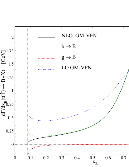
Figure 1: $d\Gamma(t(\uparrow)\rightarrow B+X)/dx_{B}$ as a function of $x_{B}$ at NLO in the GM-VFN ($m_{b}\neq 0$) scheme including finite-$m_{B}$ corrections by using Eq.(32). The NLO prediction (solid line) is compared to the LO one (dot-dashed line) and broken up into the contributions due to $b\rightarrow B$ (dotted line) and $g\rightarrow B$ (dashed line) fragmentation.

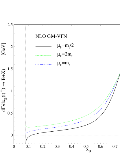
Figure 2: $d\Gamma(t(\uparrow)\rightarrow B+X)/dx_{B}$ at NLO in the GM-VFN ($m_{b}\neq 0$) scheme including finite-$m_{B}$ corrections, considering the factorization scales $\mu_{F}=m_{t}$ (dot-dashed line), $\mu_{F}=m_{t}/2$ (solid line) and $\mu_{F}=2m_{t}$ (dotted line).

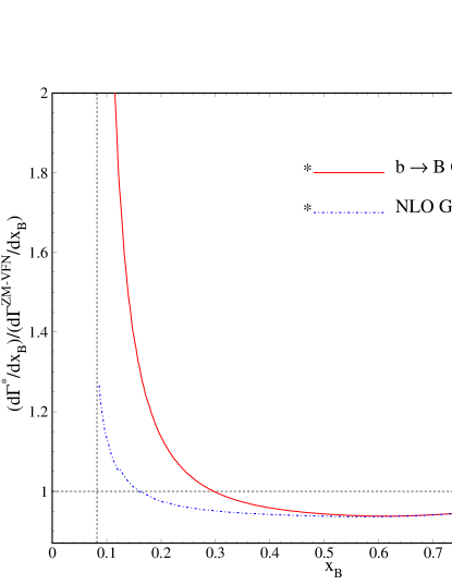
Figure 3: The result for the $d\Gamma(t(\uparrow)\rightarrow B+X)/dx_{B}$ is shown at NLO in the GM-VFN ($m_{b}\neq 0$) scheme including finite-$m_{B}$ corrections (dot-dashed line). For comparison, also the GM-VFN result excluding $g\rightarrow B$ fragmentation is shown (solid line). All results are normalized to the ZM-VFN one for $m_{B}=0$, including $g\rightarrow B$ fragmentation.

Figure 4: The ratio of the unpolarised and polarised results for the $d\Gamma(t\rightarrow B+X)/dx_{B}$ at NLO in the GM-VFN ($m_{b}\neq 0$) scheme including finite-$m_{B}$ corrections.

VII Conclusions

Studying the fundamental properties of the top quark is an object of interest in theoretical and experimental particle physics. Among other things, the LHC is a superlative top factory which allows one to study the top characteristics in great detail, if also the theoretical descriptions and simulations are of commensurate quality. In particular, the LHC will allow for the study of the dominant decay mode $t\rightarrow BW^{+}+X$ with unprecedented precision in the long run. As an application, these studies will enable us to deepen our conception of the nonperturbative aspects of B-hadron formation by hadronization and to pin down the $b\rightarrow B$ and $g\rightarrow B$ fragmentation functions. The key quantity for this purpose is the $x_{B}$ distribution $d\Gamma/dx_{B}$ of $t\rightarrow B+X$. Therefore, the distributions in the scaled B-hadron energy $x_{B}$ through the polarized (6) or unpolarized Kniehl:2012mn top decays are of particular interest at the LHC. In this context, recently, the local CMS group at the CERN LHC started to work on a determination of the top quark mass from a detailed study of the B-meson decays.
The top quark decays rapidly so that has no enough time to hadronize and then passes on its full spin information to its decay products. This allows one to study the top spin state using the angular distributions of its decay products, so that, in this work we studied the ${\cal O}(\alpha_{s})$ spin-dependent energy spectrum of hadrons produced from polarized top quark decays. For this, we studied the observable $d\Gamma/dx_{B}$ at NLO in the GM-VFN scheme Kniehl:2008zza . This allowed us to investigate, for the first time, finite-$m_{b}$ corrections to the $d\Gamma/dx_{B}$. We also analyzed the size of finite-$m_{B}$ effects. Specifically, our analysis is supposed to enhance our previous results presented in Nejad:2013fba by retaining all nonlogarithmic $m_{b}$ terms of the result in the FFN scheme. These studies are mandatory in order to fully exploit the enormous statistics of the LHC data to be taken in the long run for a high-precision determination of the top-quark properties.
Comparing future measurements of the polarized width $d\Gamma(t(\uparrow)\rightarrow BW^{+}+X)/dx_{B}$ at the LHC with our NLO predictions, one will be also able to test the universality and scaling violations of the B-hadron FFs. These measurements of the $x_{B}$ distributions will ultimately be the primary source of information on the B-hadron FFs.
Our formalism elaborated here is also applicable to the production of hadron species other than B-hadrons, such as pions, kaons and protons, etc., using the $b,g\rightarrow\pi/K/P$ FFs presented in our recent paper Soleymaninia:2013cxa , relying on their universality and scaling violations.

References

- (1) F. Abe et al. [CDF Collaboration], Phys. Rev. Lett. 74 (1995) 2626 [hep-ex/9503002].
- (2) S. Abachi et al. [D0 Collaboration], Phys. Rev. Lett. 74 (1995) 2632 [hep-ex/9503003].
- (3) V. M. Abazov et al. [D0 Collaboration], Phys. Rev. Lett. 113 (2014) 032002 [arXiv:1405.1756 [hep-ex]].
- (4) V. M. Abazov et al. [D0 Collaboration], Phys. Rev. D 85 (2012) 091104 [arXiv:1201.4156 [hep-ex]].
- (5) T. A. Aaltonen et al. [CDF Collaboration], Phys. Rev. Lett. 111 (2013) 20, 202001 [arXiv:1308.4050 [hep-ex]].
- (6) V. del Duca and E. Laenen, Int. J. Mod. Phys. A 30 (2015) 35, 1530063 [arXiv:1510.06690 [hep-ph]].
- (7) N. Cabibbo, Phys. Rev. Lett. 10 (1963) 531. M. Kobayashi and T. Maskawa, Prog. Theor. Phys. 49 (1973) 652.
- (8) K. G. Chetyrkin, R. Harlander, T. Seidensticker and M. Steinhauser, Phys. Rev. D 60 (1999) 114015 [hep-ph/9906273].
- (9) S. M. M. Nejad, Phys. Rev. D 88 (2013) 9, 094011 [arXiv:1310.5686 [hep-ph]]; S. M. Moosavi Nejad and M. Balali, Phys. Rev. D 90 (2014) 11, 114017 [arXiv:1409.1389 [hep-ph]].
- (10) G. Corcella and F. Mescia, Eur. Phys. J. C 65 (2010) 171; G. Corcella and F. Mescia, Eur. Phys. J. C 68 (2010) 687 (Erratum); S. Biswas, K. Melnikov and M. Schulze, JHEP 1008 (2010) 048, [arXiv:1006.0910 [hep-ph]].
- (11) G. Corcella and A. D. Mitov, Nucl. Phys. B 623 (2002) 247 [hep-ph/0110319].
- (12) J. C. Collins, Phys. Rev. D 58, 094002 (1998) [hep-ph/9806259].
- (13) V. N. Gribov and L. N. Lipatov, Sov. J. Nucl. Phys. 15 (1972) 438 [Yad. Fiz. 15 (1972) 781]; G. Altarelli and G. Parisi, Nucl. Phys. B 126 (1977) 298. Y. L. Dokshitzer, Sov. Phys. JETP 46 (1977) 641 [Zh. Eksp. Teor. Fiz. 73 (1977) 1216].
- (14) C. Caso et al. [Particle Data Group Collaboration], Eur. Phys. J. C 3 (1998) 1.
- (15) C. S. Li and T. C. Yuan, Phys. Rev. D 42 (1990) 3088 [Phys. Rev. D 47 (1993) 2156].
- (16) J. F. Gunion and H. E. Haber, Nucl. Phys. B 272 (1986) 1 [Nucl. Phys. B 402 (1993) 567].
- (17) J. F. Gunion, H. Haber, G. Kane, and S. Dawson, The Higgs Hunter’s Guide (Addison-Wesley, Reading, MAA, 1990), and refrences therein.
- (18) S. M. Moosavi Nejad, Phys. Rev. D 85 (2012) 054010 [arXiv:1110.1601 [hep-ph]]; S. M. Moosavi Nejad, Eur. Phys. J. C 72 (2012) 2224 [arXiv:1205.6139 [hep-ph]].
- (19) B. A. Kniehl, G. Kramer and S. M. Moosavi Nejad, Nucl. Phys. B 862 (2012) 720 [arXiv:1205.2528 [hep-ph]].
- (20) J. Binnewies, B. A. Kniehl and G. Kramer, Phys. Rev. D 58 (1998) 034016 [hep-ph/9802231].
- (21) K. Nakamura et al. [Particle Data Group Collaboration], J. Phys. G 37 (2010) 075021.
- (22) B. A. Kniehl, G. Kramer, I. Schienbein and H. Spiesberger, Phys. Rev. D 77 (2008) 014011 [arXiv:0705.4392 [hep-ph]].
- (23) M. Soleymaninia, A. N. Khorramian, S. M. Moosavi Nejad and F. Arbabifar, Phys. Rev. D 88 (2013) 5, 054019 [Phys. Rev. D 89 (2014) 3, 039901] [arXiv:1306.1612 [hep-ph]]; S. M. M. Nejad, M. Soleymaninia and A. Maktoubian, arXiv:1512.01855 [hep-ph].