A survey of classical and quantum interpretations of experiments on Josephson junctions at very low temperatures

Abstract

For decades following its introduction in 1968, the resistively and capacitively shunted junction (RCSJ) model, sometimes referred to as the Stewart-McCumber model, was successfully applied to study the dynamics of Josephson junctions embedded in a variety of superconducting circuits. In 1980 a theoretical conjecture by A.J. Leggett suggested a possible new and quite different behavior for Josephson junctions at very low temperatures. A number of experiments seemed to confirm this prediction and soon it was taken as a given that junctions at tens of millikelvins should be regarded as macroscopic quantum entities. As such, they would possess discrete levels in their effective potential wells, and would escape from those wells (with the appearance of a finite junction voltage) via a macroscopic quantum tunneling process. A zeal to pursue this new physics led to a virtual abandonment of the RCSJ model in this low temperature regime. In this paper we consider a selection of essentially prototypical experiments that were carried out with the intention of confirming aspects of anticipated macroscopic quantum behavior in Josephson junctions. We address two questions: (1) How successful is the non-quantum theory (RCSJ model) in replicating those experiments? (2) How strong is the evidence that data from these same experiments does indeed reflect macroscopic quantum behavior?

(*) Also CNR-SPIN Institute, Italy

I Introduction

The history of the Josephson junction began with Brian Josephson’s paper in 1962 Josephson . The 50th anniversary of this discovery was marked at the 2012 Applied Superconductivity Conference in Portland OR.

At its simplest, a Josephson junction consists of two superconductors separated by a very thin barrier, typically an oxide of a superconducting material. Figure 1 shows a typical thin film junction. The Nb electrodes each have a small finger, and these fingers overlap to form a Josephson junction from the sandwich of Nb top and bottom, and the oxide in between. In the most successful fabrication technology Gurwitch83 the oxide is $Al_{2}O_{3}$ thermally grown over a thin aluminum layer wetting the Nb bottom layer. The two bulk superconducting electrodes can be viewed phenomenologically as possessing separate macroscopic wavefunctions $\Psi_{1}$ and $\Psi_{2}$, as indicated in the figure, whose phase difference $\theta_{1}-\theta_{2}$ is $\varphi$. Josephson predicted that a supercurrent could flow through the junction without any associated voltage - the expression for this supercurrent being

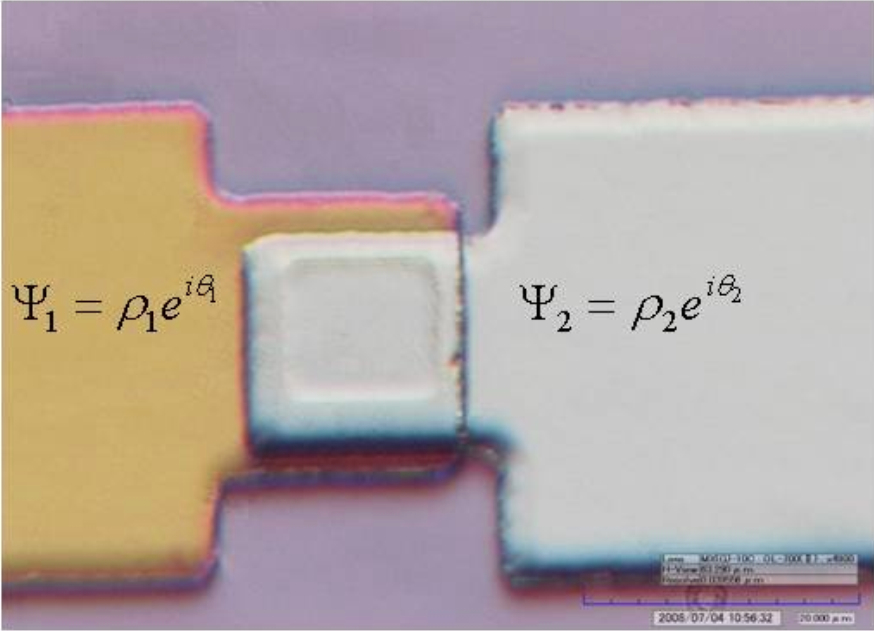
Figure 1: Photomicrograph of a thin film Josephson junction.  The small square area at the center ($10\mu m\times 10\mu m$) is the active junction.  The superconducting order parameters $\Psi$ for each film are indicated.

$$I=I_{C}\sin\varphi$$ (1)

If a voltage does exist across the junction, then the phase is governed by

$$d\varphi/dt=2eV/\hbar$$ (2)

For small junctions, those two equations comprise a complete specification of the junction dynamics. A typical current-voltage characteristic of a $Nb-Al_{2}O_{3}-Nb$ Josephson tunnel junction having a zero-voltage supercurrent of few hundreds microampères is shown in Fig. 2.

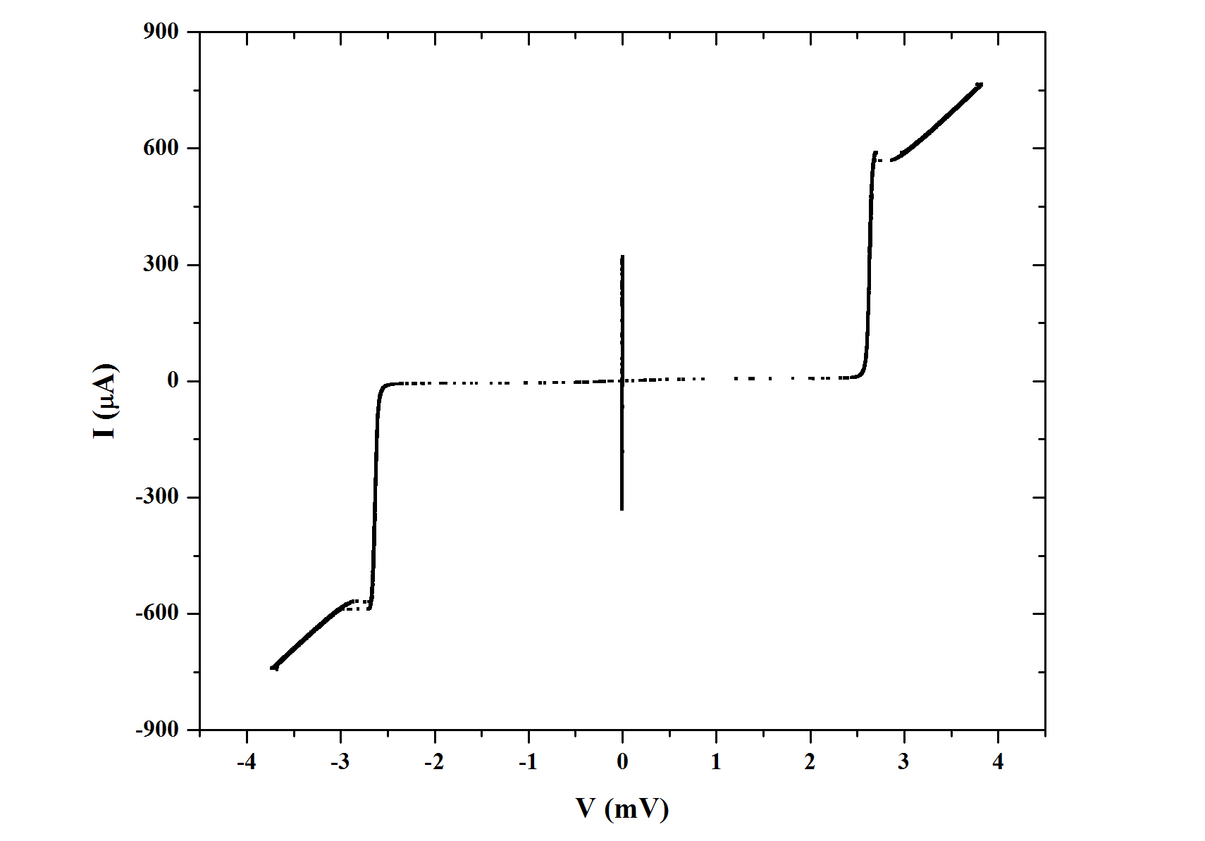
Figure 2: Typical current-voltage characteristic for an underdamped Josephson junction.

A surprising fact implied by the above equations is that the existence of the Josephson effect requires only a pair of superconducting electrodes - the choice of specific materials plays no role other than to affect the critical current $I_{C}$. As illustrated in Fig.3, this critical current rises as the junction temperature drops and saturates at low temperatures Solymar . The data in this plot are taken from Fiske and the theoretical curves are from Ambegaokar .

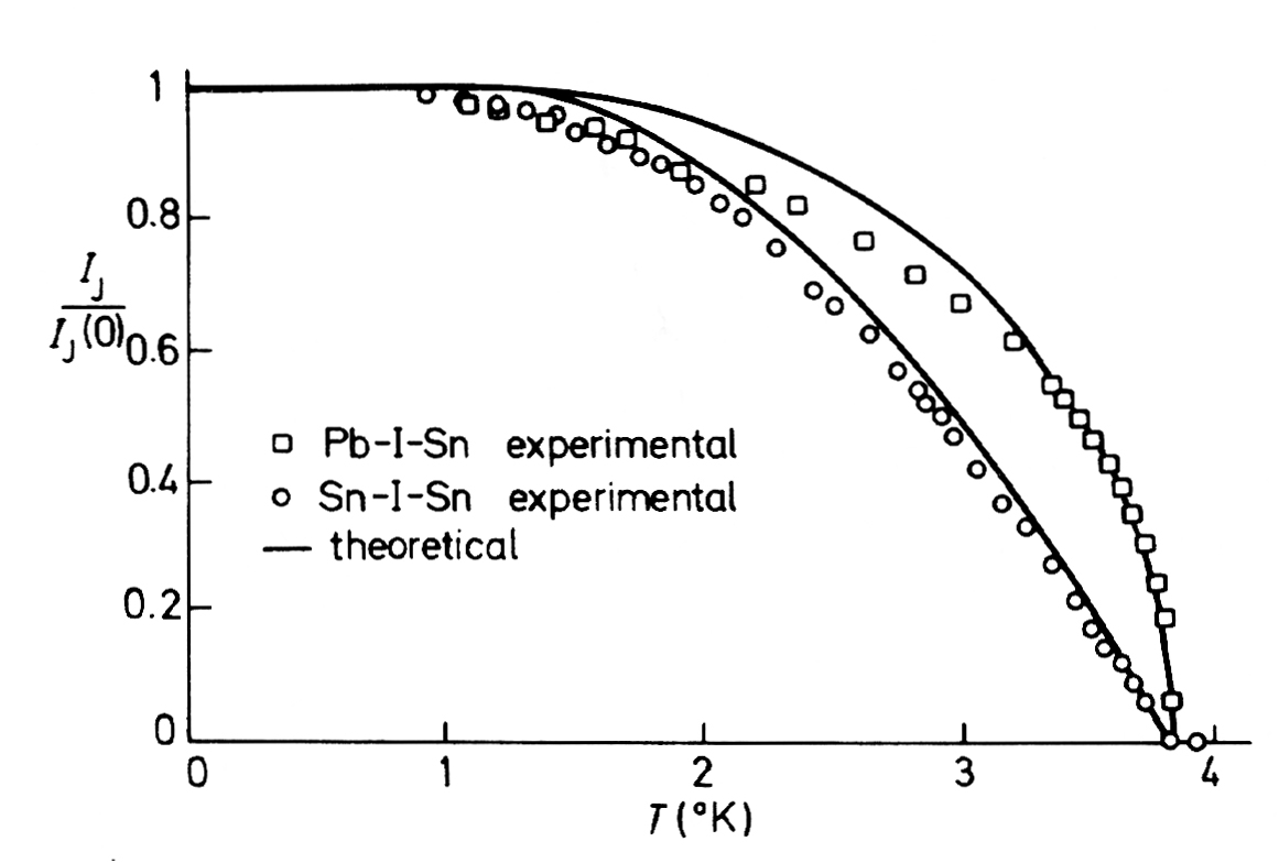
Figure 3: Variation of maximum supercurrent in a Josephson junction as a function of temperature.

Therefore, well below the transition temperature of the films there would be no additional temperature dependence in a Josephson device. Relevant and fundamental observations on the nature of the Josephson phase difference and associated energy/potential were reported by P. W. Anderson PWA64

In 1980 Leggett Leggett postulated that , at sufficiently low temperatures, the phase of a Josephson junction would take on the attributes of a macroscopic quantum coordinate. Since then, over the following decades, experimental and theoretical work has been reported demonstrating evidence that a quantum interpretation of experiments performed at low temperatures on Josephson junctions is possible. Later we will duly reference and analyze several of these experiments which are complex and sophisticated and were performed bearing in mind the idea that at very low temperatures a macroscopic quantum description was necessary.

It is our opinion, however, that decisive confirmation of the macroscopic quantum hypothesis requires an experiment (or many experiments) whose results cannot be explained in other terms. In particular, it is known that there exists (and already existed in the early 80’s indeed) a whole field of research on nonlinear circuits and applied superconductivity in which the Josephson phase is treated as a classical continuum variable in the sense specified by P. W. Anderson PWA64 . We will herein refer to this approach as the ”classical” approach. Thus the necessity of new quantum interpretation of experiments would be mandatory in case these experiments cannot be explained by the classical approach. In this Review we consider a number of key experiments that were initially claimed to unequivocally verify the quantum hypothesis. We use data extracted from those publications to very carefully reconsider the matter using the classical Josephson junction model applied to the specific conditions of each experiment.

In the next section we review shortly the features of the classical model of Josephson junctions and circuits and successively we turn to a set of essentially defining experiments and examine in detail the evidence for and against both the classical and quantum interpretations.

II The Classical Approach

II.1 RCSJ Junction Model

In the 1968 a very simple equivalent circuit, depicted in Fig.4, for a Josephson junction was proposed by W.J. Johnson (pp122-124, Barone ), D.E. McCumber, and W.C. Stewart, Stewart ; McCumber ; VanDuzer .

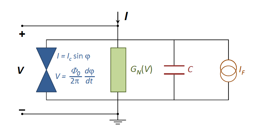
Figure 4: Resistively and capacitively shunted model of a Josephson junction (RCSJ).

This circuit Gross captures the essential ingredients of a real Josephson device. It is comprised of three parallel elements: a shunt resistor R, a shunt capacitor C, and a pure Josephson element usually labeled here with a bowtie graphic – the RCSJ model. The RCSJ equivalent circuit for a Josephson junction has proven to be exceptionally successful in modeling the dynamics of the Josephson systems.

The current through a Josephson element is given by $I$ and the voltage across the parallel combination is governed by $d\varphi/dt=2eV/\hbar$. With a total applied bias current $I$, the phase dynamics are governed by

$$\frac{\hbar C}{2e}\frac{d^{2}\varphi}{dt^{2}}+\frac{\hbar}{2eR}\frac{d\varphi}{dt}+I_{C}\sin\varphi=I$$ (3)

If time is normalized to $1/\omega_{J0}$ where $\omega_{J0}=\sqrt{2eI_{C}/\hbar C}$ is the zero-bias Josephson plasma frequency, then

$$\ddot{\varphi}+\alpha\dot{\varphi}+\sin\varphi=\eta$$ (4)

where $\eta=I/I_{C}$ is a normalized bias current and $\alpha=\frac{\hbar\omega_{J0}}{2eI_{C}R}$ is a normalized loss coefficient.

A Josephson junction with phase $\varphi$ has stored energy is $\frac{\hbar I_{C}}{2e}\left(1-\cos\varphi\right)$. The pre-factor in this expression is the Josephson energy:

$$E_{J}=\hbar I_{C}/2e$$ (5)

II.2 Washboard Potential

The total potential energy of a junction, when an additional bias current is supplied, is PWA64

$$U=E_{J}\left\{\left(1-\cos\varphi\right)-\eta\varphi\right\}$$ (6)

In this form it is apparent that the phase dynamics can be viewed in terms of a fictitious ‘particle’ whose coordinate is $\varphi$, moving in a washboard potential, as indicated in Fig.5.

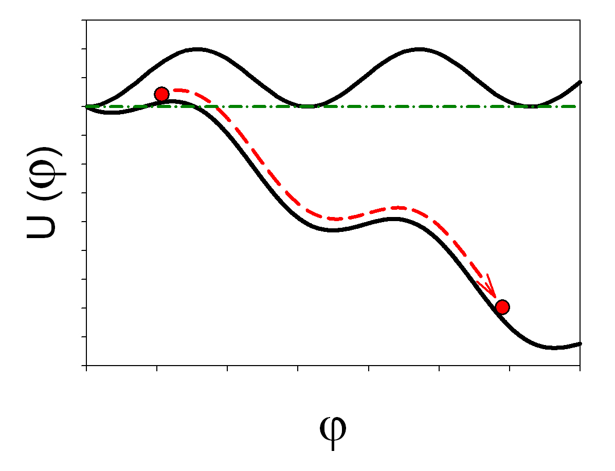
Figure 5: Washboard potential with zero bias (upper) and non-zero bias (lower).

In this analog, at zero bias the potential is a horizontal washboard and a ‘particle’ would sit at the bottom of the well at $\varphi=0$.  Small oscillations around the minimum of that well occur at the plasma frequency $f_{J0}=\omega_{J0}/2\pi$. At non-zero values of the bias: (1) the washboard tilts (2) the minimum of the well occupied by the particle shifts to $\varphi>0$ (3) the wells in the washboard potential become progressively shallower, with correspondingly smaller plasma frequencies, $f_{J}=f_{J0}\left(1-\eta^{2}\right)^{1/4}$, disappearing altogether at a bias equal to the junction critical current.

II.3 Large amplitude oscillations

For larger oscillation amplitudes, the well shape becomes increasingly anharmonic and oscillations will occur at a frequencies slightly lower than the small amplitude values given by $f_{J}=f_{J0}\left(1-\eta^{2}\right)^{1/4}$.  This can be expressed approximately as

$$f_{J}=f_{J0}\sqrt{\;\left[J_{0}(a)+J_{2}(a)\right]\sqrt{1-\left(\frac{\eta}{J_{0}(a)}\right)^{2}}}$$ (7)

where $J_{0}$ and $J_{2}$ are Bessel functions of the first kind and $a$ is the amplitude of the oscillation. A ‘large’ amplitude oscillation would take the phase from the minimum position of a well to the inflection point of that well. In this case the amplitude can be approximated by

$$a\approx\sqrt{\frac{4}{3}\left(1-\eta\right)}$$ (8)

(see NGJ2 ). At the critical bias $\eta=1$, $a=0$ and $f_{J}=0$. For bias currents less than unity, the anharmonic plasma frequency is slightly smaller than the harmonic value.

II.4 Escape from a well

The barrier height $\Delta U$ for the washboard potential, indicated in Fig 6, is controlled by the bias current $\eta$ and is given by Eq.9

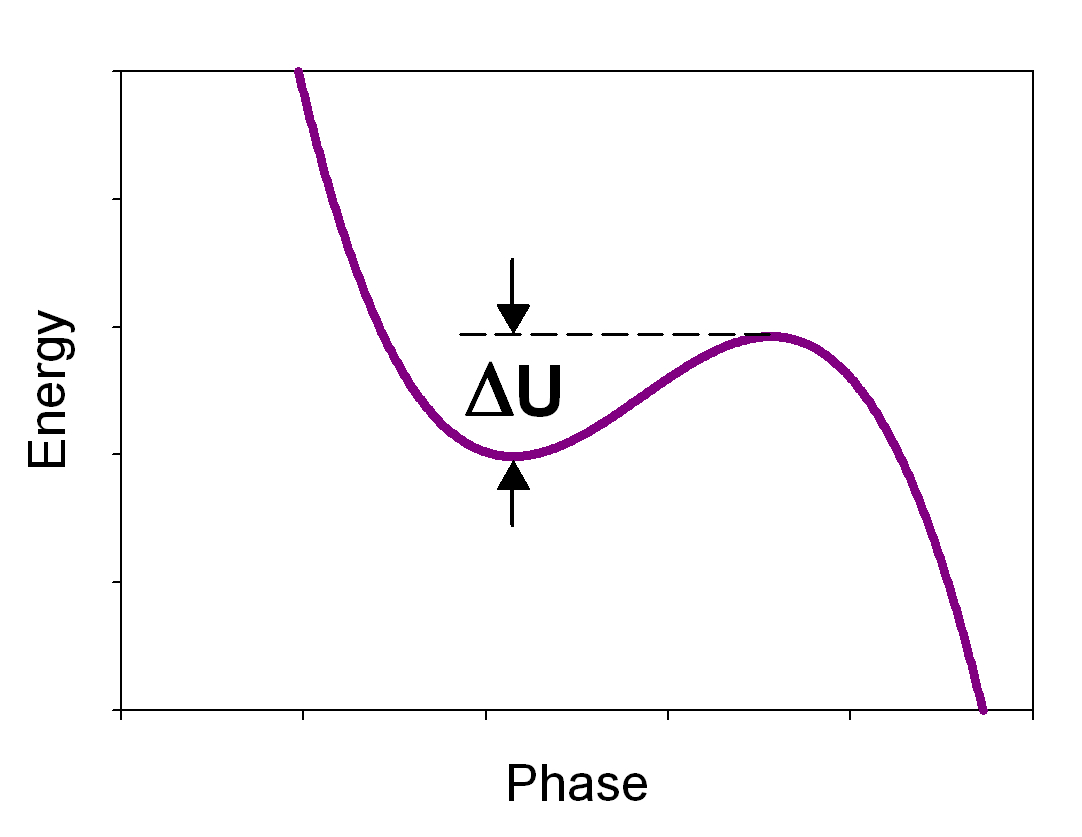
Figure 6: Portion of washboard potential illustrating the barrier for escape.

$$\Delta U=2E_{J}\left[\sqrt{\left(1-\eta^{2}\right)}-\eta\cos^{-1}\eta\right]$$ (9)

If noise is present, then the ‘particle’ can hop out of the well and bounce down the washboard, as illustrated above. For thermal activation, the escape rate at temperature $T$ is given by

$$\Gamma(t)=f\exp\left(\frac{-\Delta U}{k_{B}T}\right)$$ (10)

where $f$ is an attempt frequency. So if a constant bias is applied, escape is inevitable, but for a shallow well it will happen sooner than for a deep well.

Because $d\varphi/dt=2eV/\hbar$, this bouncing motion is accompanied by an oscillating but always positive junction voltage.

Modeling some types of experiment, those involving junctions in superconducting circuits, can be done by determining the junction phase dynamics from Eq. 3 while other types, those based on activation processes, can be addressed with Eq. 4.

II.5 Pendulum Analog

Equation 3 is isomorphic to the equation that governs the motion of a driven pendulum, as depicted in Fig.7.

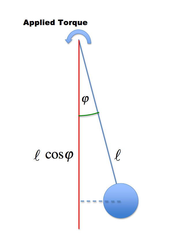
Figure 7: A simple pendulum.

For the pendulum, the equation of motion is

$$I\,\ddot{\varphi}+\gamma\dot{\varphi}+mg\ell\sin\varphi=\Gamma$$ (11)

where $m$ is the mass of the bob, $\ell$ is the length of the suspension, $I$ is the rotational moment of inertia ($m\ell^{2}$ in the case of a simple pendulum), $\gamma$ is the damping, and $\Gamma$ is the net appied torque.  The potential energy of this system for a displacement angle $\varphi$ and an applied torque $\Gamma$ is

$$U=mg\ell(1-\cos\varphi)+\Gamma\varphi$$ (12)

This, of course, is the washboard potential of Eq.6 and Fig.5.  A mechanical analog such as this helps to visualize the behavior of a Josephson junction.  For example, increasing the applied torque will increase the pendulum angle until it reaches $\pi/2$ at which point a minute additional applied twist, or noise, will cause the pendulum to flip over the top and then spin - i.e. bounce down the washboard.  This critical torque, $\Gamma_{C}=mg\ell$, plays the role of the critical current $I_{C}$ in the junction.

Also, at zero-torque the frequency of small oscillations about the down position is the familiar $f_{0}=\frac{1}{2\pi}\sqrt{g/\ell}$. which is the analog of the Josephson zero-bias plasma frequency with the correspondence: $\hslash C/2e\Leftrightarrow m\ell^{2}$. But if these oscillations have a large motion side-to-side with an amplitude $\theta$ then the period becomes

$$P=4\sqrt{\frac{\ell}{g}}\int_{0}^{\pi/2}\frac{d\theta}{\sqrt{1-k^{2}\sin^{2}(\theta)}}$$ (13)

where the right hand side is an elliptic integral of the first kind (see elliptic ). This period becomes larger than the small angle value as the amplitude of the oscillations increases, and so the anharmonic frequency diminishes accordingly.

The analog of a constant current bias of a Josephson junction is a constant torque applied to the pendulum. For any applied torque $0<\Gamma<\Gamma_{C}$, the pendulum will have a stable position at an angle somewhere between $0$ and $\pi/2$.  Any perturbation will cause oscillations around that stable point.  As with the Josephson junction, the frequency of small oscillations would scale with the applied torque.

$$f_{P}=f_{0}\sqrt[4]{1-\left(\Gamma/\Gamma_{C}\right)^{2}}$$ (14)

But for larger induced oscillations around the stable angle, an expression similar to Eq.7 would apply.

II.6 Switching Current Distributions

The usual experimental approach to measuring activation involves sweeping the bias current upward from zero. Early in the sweep, the well is deep; late in the sweep the well becomes quite shallow. Thermal activation is easier from a shallow well. But in addition, as the bias is swept, the plasma frequency drops and thus the rate of escape attempts decreases. The interplay of these two factors determines the net escape rate for the momentary bias current.

When the bias current is repeatedly ramped up from zero, at a given temperature, for each sweep the value of the bias current when the junction switches to the finite voltage state is recorded. The distribution of these accumulated escape events forms a Switching Current Distribution (SCD) peak whose two key attributes are position and width; this is the primary form of experimental data.

A method for simulating the escape process seen in an experiment was described in Blackburn1 . The method begins with an ensemble of $M$ junctions. The bias on all junctions starts at $0$ and is incremented in $N$ steps, with each step of duration $\Delta t=\left(Nf_{S}\right)^{-1}$, where $f_{S}$ is the sweep frequency. Each step is assigned a channel, and the total counts in that channel indicates how many junctions have switched to the finite-voltage state (escaped from a potential well) during that interval. As the bias sweep proceeds, the original ensemble will have lost $e_{1}$ junctions in the first interval, $e_{2}$ junctions in the second interval, and so forth. Consequently, at the beginning of the $n^{th}$ bias interval, there will be $M-\sum_{j=1}^{n-1}e_{j}$ junctions not yet escaped. The number from this remaining pool of junctions that will escape during the next interval$\Delta t$ will be

$$e_{n}=\left[M-\sum_{j=1}^{n-1}e_{j}\right]\,\Gamma(t_{n})\Delta t,\quad n=2,3\cdots N$$ (15)

where $\Gamma(t_{n})$ is the probability of escape per unit time in the $n^{th}$ interval. Of course, the initial interval just satisfies:

$$e_{1}=M\Gamma(t_{1})\Delta t$$ (16)

These two equations will mimic a swept-bias experiment provided a suitable expression is available for the escape rate $\Gamma$.

For the case of thermal activation (TA) out of the potential well at the $n^{th}$stage, the escape rate is

$$\Gamma(t_{n})=f_{n}\exp\left(\frac{-\Delta U_{n}}{k_{B}T}\right)$$ (17)

where $f_{n}$ is the Josephson plasma frequency in the $n^{th}$ bias interval and $\Delta U_{n}/k_{B}T$ is the height of the potential barrier divided by the mean thermal energy.

So from Eq. 4 with $\eta_{n}$ indicating the bias current at the $n^{th}$ step normalized to the junction critical current,

$$\Delta U_{n}=2E_{J}\left[\sqrt{1-\eta_{n}^{2}}-\eta_{n}\cos^{-1}\eta_{n}\right]$$ (18)

To perform a simulation, only three parameters must be known: the critical current of the junction $I_{C}$, the bias sweep frequency $f_{S}$, and the temperature $T$. Values must be chosen for the number of channels $N$ and for the ensemble number $M$ ; these are arbitrary – large numbers improve precision but slow the computation slightly. Typical choices were: $N=5000\;\,M=100,000$.

It is worth noting that a number of papers reported on successful investigations of potentials of specific Josephson junctions systems by using thermal escape techniques in parallel with RCSJ simulations. These analyses were concerned with extended Josephson junctions Kautz , dc-SQUID systems NGJ0 and step-edge junctions Barb of high Tc superconductors.

III The Classical to Quantum Crossover

The concept of crossover temperature was introduced by Affleck Affleck in the attempt to distinguish between classical and quantum fluctuations in one-dimensional potentials  In terms of Josephson quantum narrative, in the vicinity of the crossover temperature, the mechanism for escape to a finite voltage state changes from thermal activation (TA) to macroscopic quantum tunneling (MQT). Because the MQT tunneling rate is not temperature dependent, the position and width of SCD peaks must both saturate at low temperatures.

As discussed earlier, the classical escape rate for thermal activation is $\Gamma=f_{J}\exp\left(-\frac{\Delta U}{k_{B}T}\right)$ . For the case of escape via macroscopic quantum tunneling, the rate is given by (see e.g., Devoret ).

$$\begin{array}[]{l}{\Gamma_{q}=a_{q}\;f_{J}\exp\left[-7.2\frac{\Delta U}{hf_{J}}\left(1+\frac{0.87}{Q}\right)\right]}\\ {a_{q}\approx\left[120\pi\left(\frac{7.2\Delta U}{hf_{J}}\right)\right]^{1/2}}\end{array}$$ (19)

The crossover temperature may be defined by the condition that the escape rate for thermal activation equals the escape rate for MQT, which is

$$f_{J}\exp\left(\frac{-\Delta U}{k_{B}T}\right)=a_{q}\;f_{J}\exp\left[-7.2\frac{\Delta U}{hf_{J}}\left(1+\frac{0.87}{Q}\right)\right]$$ (20)

and so

$$\frac{\Delta U}{k_{B}T}\approx 7.2\frac{\Delta U}{hf_{J}}$$ (21)

with the usual assumptions: $a_{q}\approx 1$ and$Q\gg 1$. Therefore

$$T_{cr}=\frac{hf_{J}}{7.2k_{B}}$$ (22)

The Josephson plasma frequency is bias-dependent because the curvature of the well is also bias-dependent. For example, in the harmonic approximation, $\ f_{J}=f_{J0}\left(1-\eta^{2}\right)^{1/4}$.

Switching current distributions (SCD) are acquired by repeatedly sweeping the bias current at a specified temperature; consequently throughout any scan the TA escape rate varies only because of the changing bias. For each temperature, there will be a different SCD peak. In comparison, because the MQT escape rate is independent of temperature, only a single peak should be seen. Figure 8 shows simulation results based on experimental data from Yu .

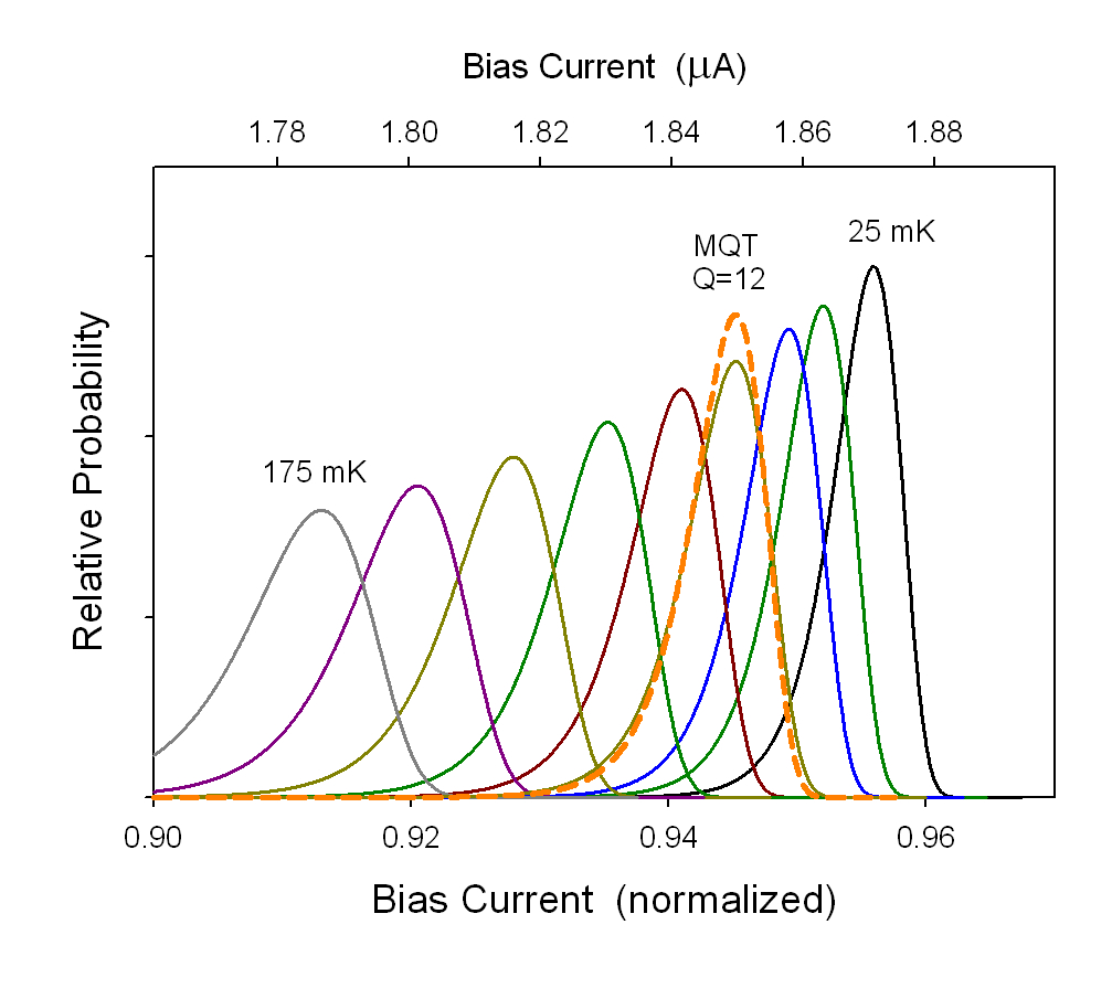
Figure 8: Results of two simulations using the parameters of the sample in Yu . One simulation utilized the thermal activation (TA) escape rate, while the other used the macroscopic tunneling (MQT) escape rate, Eq.19. The MQT peak coincides with the particular TA peak for $65$ mK.

It can be seen that the MQT SCD peak falls exactly on a TA SCD peak at just one particular temperature – that defines the crossover temperature. Note that the value of the bias of this special peak is not zero, and so the plasma frequency $f_{J}$ will be smaller than $f_{J0}$. Because any peak position is never known a priori, the expression for the crossover temperature can only be used as an approximation with $f_{J}\approx f_{J0}$. Suppose for example, an experimental SCSD peak happened to occur at a normalized bias of $0.9$.  Then $\left(1-0.9^{2}\right)^{1/4}=0.66$ and so the anticipated crossover temperature would be a fraction of the value obtained using $\ f_{Jo}$. Taking as an example a crossover temperature quoted at $60$ mK, the ‘true’ value could be $40$ mK. The higher the peak position, the larger the discrepancy. Most cryostats bottom out at around $20$ mK meaning the acquired data do not reach very far below the presumed crossover value. We conclude that there is not much room to show unambiguous experimental confirmation of an MQT transition in Josephson junctions.

III.1 Experimental Evidence

Voss and Webb

The pivotal moment in the history of switching current distributions measured at millikelvin temperatures was the 1981 paper by Voss and Webb VossWebb . They presented experimentally recorded SCD peaks for 11 selected temperatures. Their figure is shown here (Fig 9) together with results from an RCSJ simulation based on the thermal-activation escape rate given in Eq.17.

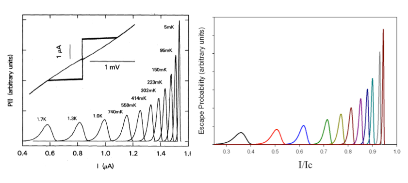
Figure 9: Experimental results from VossWebb for SCD peaks at various temperatures; Right: RCSJ simulation results

The simulation is clearly in excellent agreement with experiment, but a precise test is not possible because full details of the bias sweep were not given; the text says only that “A low-frequency sinusoidal current (amplitude $\approx 2I_{C}$) was applied to the junction and the distribution of currents at which the junction switched out of the superconducting state was measured”. The current-sweeps were stipulated as being in the range $10-20\,Hz$. Peak positions, especially at high bias values, are known to be sensitive to the shape and speed of the bias sweep.

The peak width data from Voss and Webb VossWebb for the sample with critical current $1.62{\;}\mu A$ are shown in Fig.10. Note the choice of a log scale for temperature. Again, this set the standard for presentations of experimental data (however see the Appendix). From this figure data points were extracted and then re-plotted as shown in the right panel.

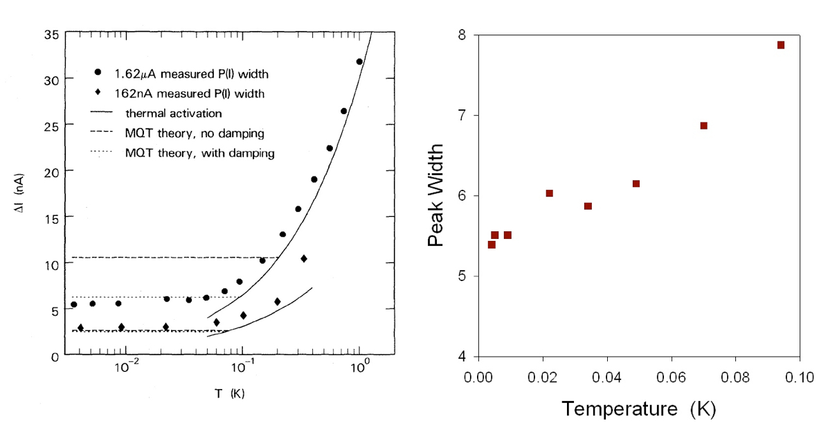
Figure 10: Left: Experimental data of VossWebb ; Right: Expanded view of data on the left at the lowest temperatures and with a linear temperature scale.

This illustrates a crucial point: the choice of a logarithmic temperature axis makes it appear that there is a flattening. The linear plot of the same data, shown here, makes it very clear that saturation of the peak width below $100\,mK$ has not occurred. The fact that the trend in the data is not towards the origin is discussed in the section: Effective Temperature.

Since the paper by Voss and Webb VossWebb , many other swept bias experiments have been reported. A typical example from three decades later is the following.

Yu et al.

Yu et al. Yu carried out swept bias experiments on a junction with a critical current of $I_{C}=1.957\,\mu A$ and a bias sweep rate of $0.4$ mA/s; the observed SCD peaks are shown in Fig.11. An RCSJ simulation was applied to this experiment Blackburn3 ; representative simulation SCD peaks are also shown.

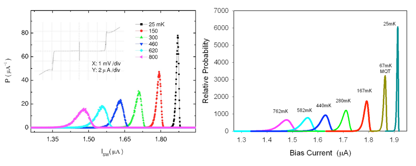
Figure 11: Left: Experimental results for swept bias escape peaks from Yu ; Right: RCSJ simulation results for escape peaks.

From figure 2 in Yu the experimental peak positions (blue squares) were digitized and are plotted in Figure 12.  Clearly, there is a suggestion of levelling off at low temperatures, however this impression is exaggerated by the choice of a logarithmic temperature scale.

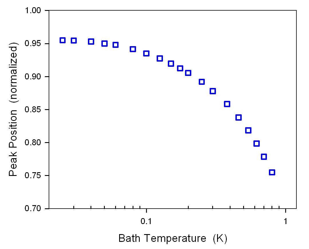
Figure 12: SCD peak position data as presented in Fig.2 of Yu .

III.2 Effective Temperature

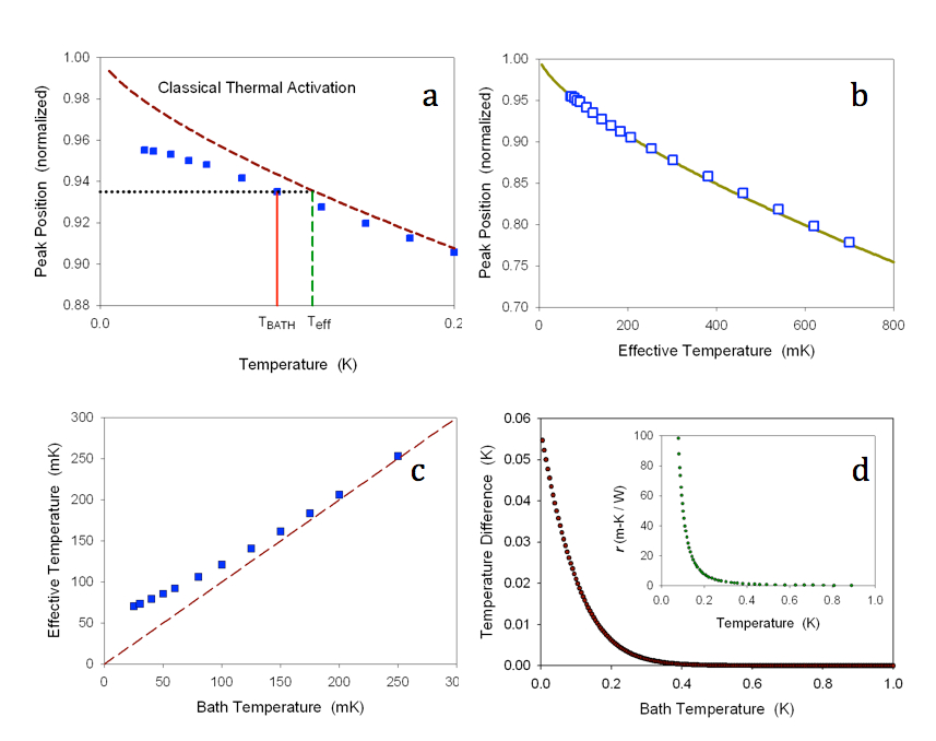
Figure 13: (a) Experimental data from the preceding figure (squares) plotted with a linear temperature scale, and the corresponding results from a simulation based thermel activation model. The constuction lines indicate how a corrected sample temperature can be inferred. (b) Experimentalpeak positions plotted versus effective sample temperature (c) Effective sample temperature versus bath temperature. (d) Comparison of the temperature elevation implied by the effective temperature with thermal resistivity data for niobium (inset)

Just replacing the log scale with a linear scale produces the result shown in Fig.13 (a). Clearly the peak positions deviate from the expectations of a fully classical TA escape process (dashed line) and the deviation increases as the temperature is lowered. Nevertheless, it is quite apparent that the peak positions have not decisively saturated at the lowest temperatures. A resolution of this difficulty can be found in choosing any specific peak, and noticing that the experimentally reported temperature is not the same as the temperature of an identical classical peak, as indicated by the construction lines in Fig.13 (a).

In other words, it is the effective sample temperature that ought to be used in the escape rate

$$\Gamma(t_{n})=f_{n}\exp\left(\frac{\Delta U_{n}}{k_{B}T_{eff}}\right)$$ (23)

to give correct peak positions (and widths). Our definition of $T_{eff}$ is essentially the same as the escape temperature $T_{esc}$ introduced in 1985 by Devoret, Martinis, and Clarke Devoret and repeated in several subsequent papers. With the bath temperature replaced by the effective temperature, the earlier plot changes to Fig.13(b) which shows excellent agreement between experimental data and predictions of thermal activation theory.

The experimentally reported temperatures are, in reality, the measured mixing chamber temperatures. The effective temperatures refer to the junctions themselves. A plot of $T_{eff}\,vs\,T_{BATH}$ (see Fig.13 (c)) highlights the degree to which the junction temperature rises above the bath temperature.

Even more revealing is a plot, Fig.13 (d), derived from the previous graph, of the difference between the effective (junction) temperature and the bath temperature as a function of bath temperature. The junction temperature is seen to begin rising above the bath temperature below about $300mK$ and this behavior is mirrored in the temperature dependence of the thermal resistivity of niobium (inset). One could infer from these plots that the apparent rise of the junction temperature might be connected to the increasing thermal resistance of the thermal path from junction to bath.

The paper by Voss and Webb in 1981 indeed launched a field of study; its importance was that it seemed to show for the first time (in Fig.3) clear evidence that “Below $100$ mK the distribution widths become independent of $T$” and that “The results are in excellent agreement with predictions for the quantum tunneling of the (macroscopic) junction phase …”, in other words, that MQT had been confirmed.

Figure 14 is an expanded view of experimental data points from Yu et al.Yu . Both axes are linear in contrast to a log temperature scale which, as was pointed out earlier, tends to stretch the data along the temperature axis and create the appearance of a saturation of the peak positions as the lowest temperatures are approached. The dashed line is drawn at the peak position indicated by Yu et al. as the expected quantum limit.

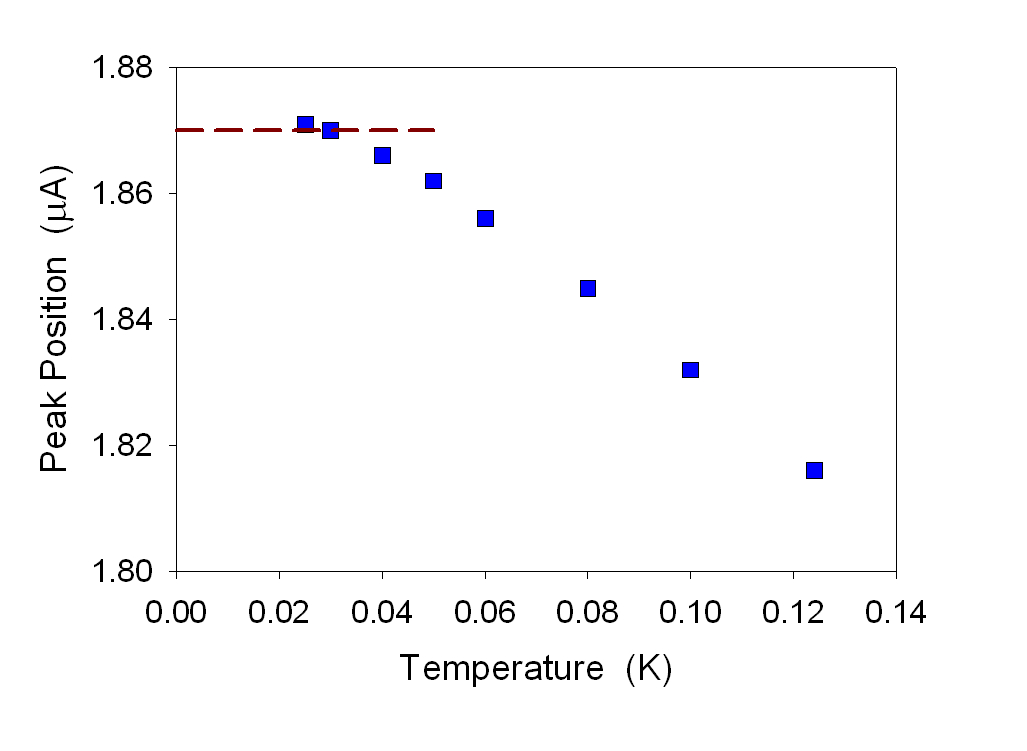
Figure 14: Expanded portion of SCD peak position data from figure 2 in Yu but with a linear temperature scale. The horizontal dashed line is the MQT prediction according to Yu .

It is quite apparent that the peak positions have not become temperature independent, and no evidence of an MQT transition can be claimed.

A recent investigation of transmon qubits Jin considered the possibility that a superconducting qubit might not be in equilibrium with its cryogenic environment, leading to effective temperatures in the range $50-130mK$.

III.3 Escape Temperature

In 1985, Devoret et al. Devoret introduced the concept of an escape temperature, defined by the expression

$$\Gamma=\frac{\omega_{J}}{2\pi}\exp\left(-\frac{\Delta U}{k_{B}T_{esc}}\right)$$ (24)

From their experimental data for the positions of the escape peaks at a each bath temperature, the escape rate was determined. Then, $T_{esc}$was calculated from the above equation. In other words, they asked: what revised junction temperature would yield agreement with the experimental observations of escape peak positions? This in fact is exactly the question posed in our discussion of SCD peaks in the RCSJ model. So the escape temperature here is the effective temperature in the earlier discussion.

Their plot showing the relationship between escape temperature and bath temperature is reproduced here in Fig.15.

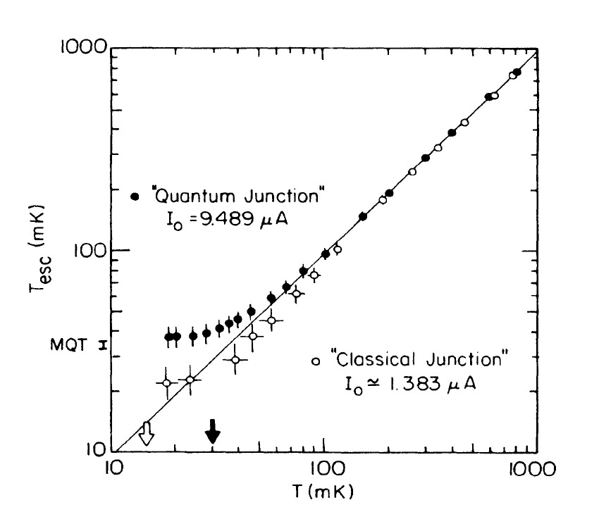
Figure 15: Plot of escape temperature versus bath temperature as reported in Martinis .

In the limit $T\to 0$, the escape rate is expected to be entirely due to MQT and therefore

$$T_{esc}\rightarrow\frac{\hbar\omega_{J}}{7.2k_{B}\left(1+0.87/Q\right)}$$ (25)

For their high critical current junction, they indicate that the escape temperature was expected to be $36$ mK, as marked by the label ‘MQT’.

The calculation can be inverted by substituting this value of $T_{esc}$ in the expression and asking what plasma frequency is implied. For $Q=30$ the conclusion is that to make this work, the plasma frequency must be $\omega_{J}=35.9\times 10^{9}$ or $f_{J}=5.71\,GHz$. However, the zero-bias plasma frequency $\omega_{J0}=\sqrt{2eI_{C}/\hbar C}$ equals $67.4\times 10^{9}$ using the stated values $I_{C}=9.489\mu A$ and $C=6.35\,pF$; thus $f_{J0}=10.72\,GHz$. Hence the apparent fit to the experimental data in the $T\to 0$ limit is a result of choosing a plasma frequency approximately half the zero-bias value. That drop in value would occur at a normalized bias of $0.9375$. But what justification is there for this value? In Devoret et al. the claim was made that all of this is achieved “with no adjustable parameters”, but it seems the plasma frequency was selected to achieve the desired limit.

An important point to note is that each of the points in this plot came from finding an escape temperature that matched the observed escape rate $\Gamma$. There is nothing intrinsically quantum in such a calculation. Only the limiting value ($T\to 0$) is a prediction of MQT, not the data points at finite temperature.

This particular plot first appeared in Devoret, Martinis, and Clarke (1985) Devoret , and the exact same figure appeared also in Martinis, Devoret, and Clarke (1987) Devoret and yet again in Clarke, Cleland, Devoret, Esteve, and Martinis (1988) Devoret . It might also be noted that the “Classical Junction” was just the “Quantum Junction” with an applied magnetic field used to reduce the critical current from $9.489\mu A$ to $1.383\mu A$, so in fact only one experimental sample was involved in all these claims of observing MQT effects.

As was done in the earlier discussion of the RCSJ model applied to such experiments, an alternate graphical presentation (Fig.16) hints at another interpretation.

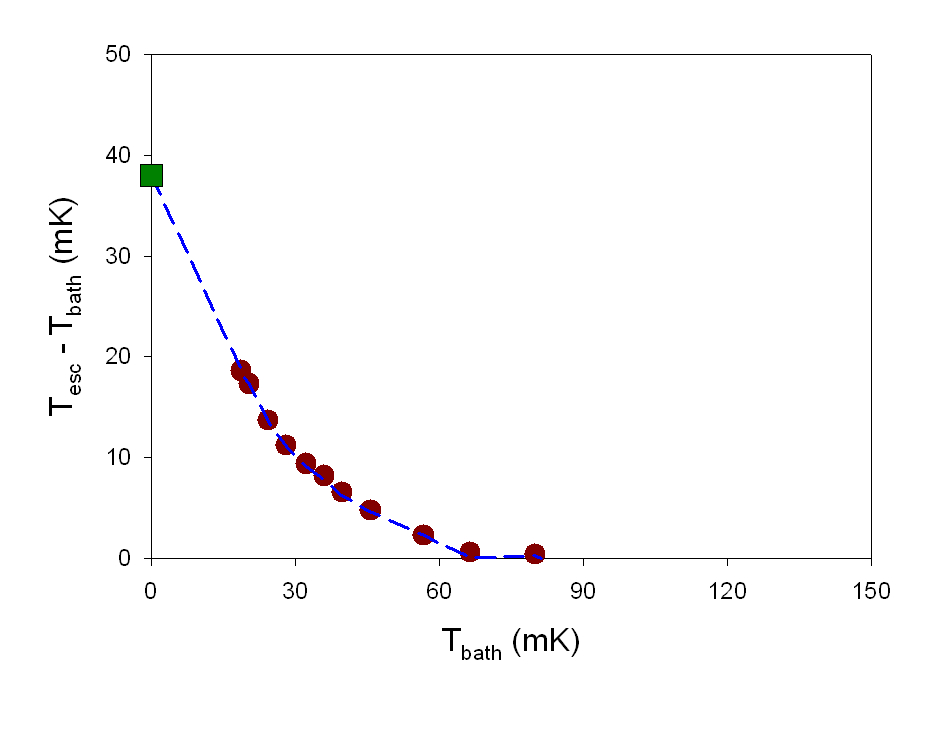
Figure 16: Data from Fig.15 replotted to show the elevation of sample temperature as a function of bath temperature.

Taking all the data points and not focusing entirely on the limiting value, it becomes apparent, as discussed for the RCSJ interpretation of the data of Yu et al., that the sample temperature appears to rise above the bath temperature, Martinis et al. (1987) Devoret were obviously aware of this issue when they stated: “Although the low-temperature values of $T_{esc}$ plotted in Fig. 2 are in good agreement with the $T=0$ prediction, nevertheless one should demonstrate that the flattening of $T_{esc}$ is not due to an unknown, spurious noise source.”

This crucial point was raised by Cristiano and Silvestrini Cristiano who noted that in the presence of external noise, the effective temperature can be higher than the bath temperature. This matter was debated in an exchange in Physical Review Letters 1989 Silvestrini2 ; Devoret2 . In a subsequent paper on the topic of escape temperature, Silvestrini Silvestrini aptly remarked: “From a theoretical point of view, $T_{esc}$ is then a good variable to clearly visualize the transition between the classical and quantum limit, if there is any” and then “From an experimental point of view, on the contrary, $T_{esc}$ is not a direct measured quantity but strongly correlated to junction parameters which are not known a priori, as the critical current $I_{C}$ , the junction effective resistance and capacitance.” And in fact Devoret et al. (1985) Devoret did concede that “the error in the predicted value of $T_{esc}$ arises predominantly from uncertainties in $\omega_{P}$ and $Q$ ”.

A definitive resolution of the dispute would be to directly measure the junction temperature during the experiment instead of measuring the bath temperature. Then one would know for certain if the escape temperature did or did not indicate an MQT escape process at work. Otherwise, as is obvious, there remains a ‘loophole’ in the logic because evidence that no noise is present is indirect and possibly not applicable to the many other similar experiments that also claim to see MQT.

Finally, in their Reply to Silvestrini’s Comment, Devoret et al.Devoret conceded that: “It is of course true that, as Silvestrini states, our data “do not represent an unambiguous proof of MQT”.

IV Classical Resonances and Quantum Levels

IV.1 Classical Resonances

In terms of RCSJ model the phase dynamics of a Josephson junction are governed by equation 3. For small amplitude oscillations in the washboard potential well, the natural frequency is $f_{J}=f_{J0}\left(1-\eta^{2}\right)^{1/4}$. In the anharmonic approximation, larger amplitude oscillations occur at a frequency given by Eq.7.

When both dc and ac bias currents are applied, the phase equation becomes

$$\ddot{\varphi}+\alpha\dot{\varphi}+\sin\varphi=\eta+\eta_{ac}\sin\left(\omega t\right)$$ (26)

The ac forcing term mimics the presence of external microwaves irradiating the junction. As an illustrative example, the following junction parameters were chosen: $I_{C}=9.489\mu A$,$C=6.35pF$, giving a zero-bias plasma frequency of $10.72\,GHz$ The above was solved numerically Blackburn2 , see Fig.17, under the following conditions: the dissipation constant was set at $\alpha=0.00845$ and the dc bias current was fixed, in this case at $0.9895$. For each selected ac bias frequency, the excitation amplitude $\eta_{ac}$ was ramped up from zero to approximately $0.001$ over a time interval of $600$ plasma periods. The maximum amplitude of the resulting oscillations in $\varphi$ on the escape side of the well was noted.

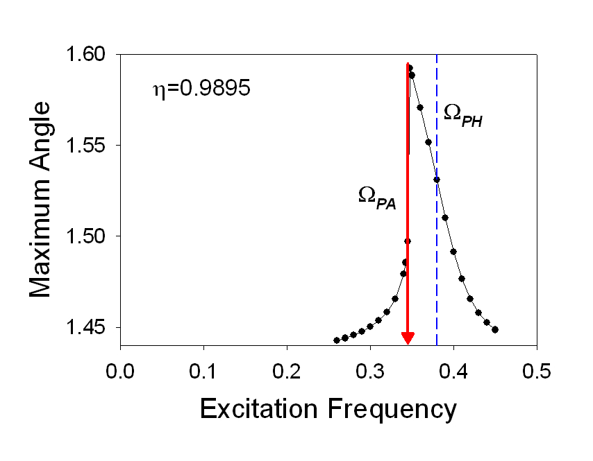
Figure 17: Maximum amplitude, on the barrier side of the well, of induced phase oscillations as a function of the frequency of excitation. Dots: numerical simulation, $\Omega_{PH}$ is the plasma frequency in the harmonic approximation, $\Omega_{PA}$ is the plasma frequency in the anharmonic approximation.

This response curve shows clearly that the amplitude of the induced phase oscillations is a maximum when the excitation frequency matches the plasma frequency as determined by the anharmonic approximation (marked by a black triangle). The plasma frequency calculated from the harmonic approximation (dashed line) lies slightly above that value and has slightly smaller induced oscillations.

To carry out a full simulation of a swept bias experiment, the previous method (no microwaves) must be adapted to the present case. The essential idea is to modify the previous escape rate (at the $n^{th}$ step in the bias sweep)

$$\Gamma(t_{n})=f_{n}\exp\left(\frac{-\Delta U_{n}}{k_{B}T}\right)$$ (27)

so as to account for the lowering of the barrier by the resonant excitation. Whenever sustained phase oscillations are induced, energy is pumped into the system.

As figure 18 suggests, the maximum induced phase excursion $\delta\varphi_{n}$ on the escape side of the well that exists at the $n^{th\text{ }}$bias step leads to an effective barrier that is smaller than the full height $\Delta U_{n}$:

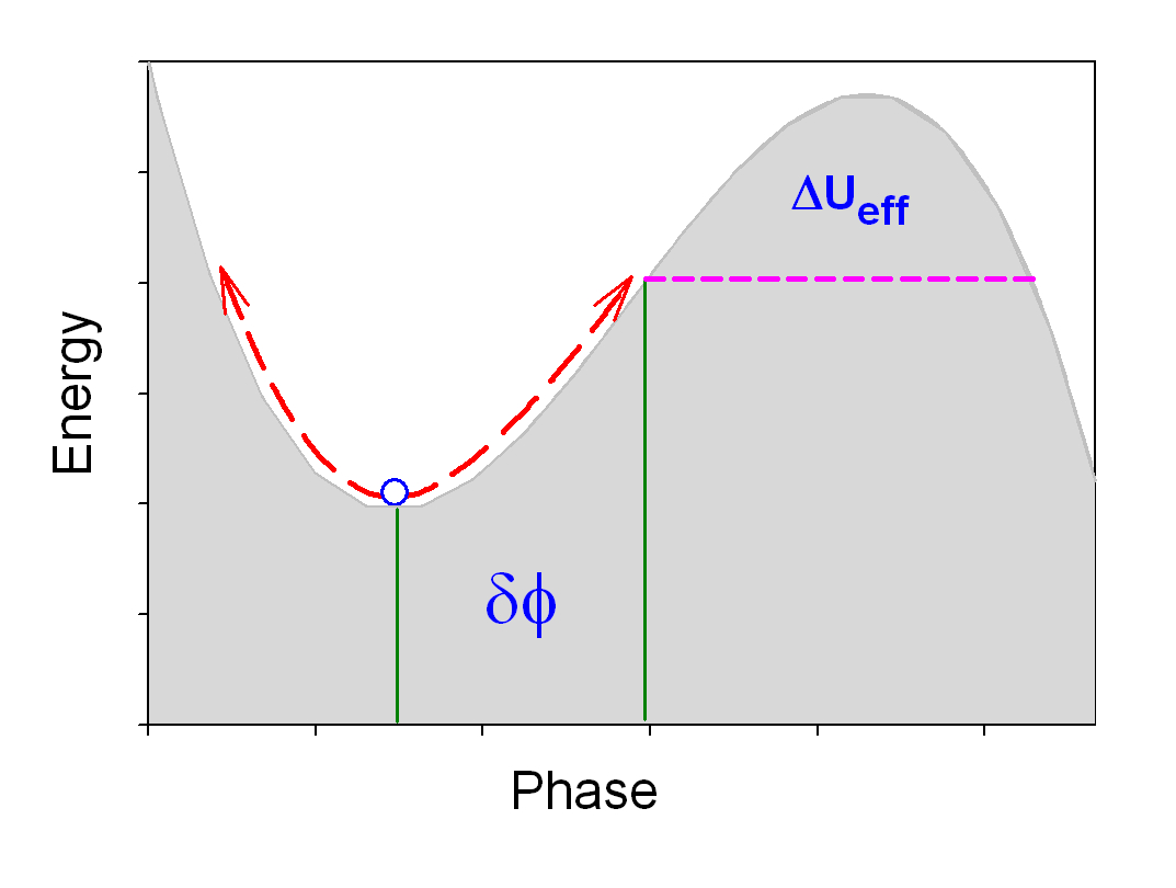
Figure 18: Induced oscillations of a ”particle” in the washboard potential well.  The reduced escape barrier $\Delta U_{eff}$  is indicated.

$$\frac{\Delta U_{eff}}{k_{B}T}=\frac{\Delta U_{n}}{k_{B}T}-\frac{\Delta U_{pump}}{k_{B}T}$$ (28)

It is reasonable to suppose that ac induced phase oscillations would take the form

$$\delta\varphi_{n}=a\frac{b^{2}}{\left(\eta_{n}-\eta_{res}\right)^{2}+b^{2}},$$ (29)

In other words, a Lorentzian distribution centered on the resonance mentioned earlier – $\eta_{res}$ being the anharmonic bias value.

The pump energy can be calculated from the value of the phase at the bottom of the well together with $\delta\varphi_{n}$. With this modification to the barrier height, the revised escape rate can be used exactly as in the earlier simulation of swept bias experiments without microwaves.

IV.2 Quantum Levels

The potential energy of a Josephson junction $U(\varphi)$ is given by Eq.6 and is plotted in Fig.19. The macroscopic quantum conjecture is that well below the crossover temperature the phase of a Josephson junction $\varphi$ becomes the coordinate of a quantum ‘particle’ existing within a potential well which can contain discrete energy levels. The wavefunctions of the ground state and first two excited states, calculated numerically Wallraff2 , are shown.  If  true, a Josephson junction would be a macroscopic object with atom-like energy states You .

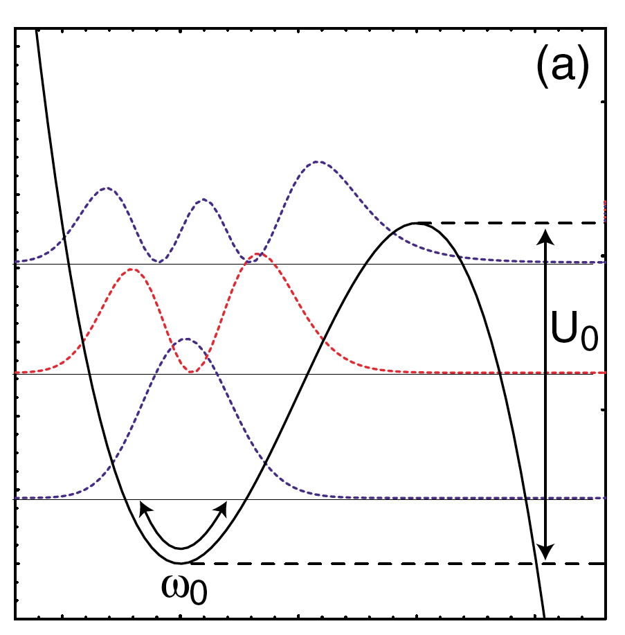
Figure 19: First three quantum wavefunctions in the potential of a Josephson junction (from Wallraff2 ). The solid curve is $U(\varphi)$ versus $\varphi$. The barrier height is $U_{0}$ and the zero-bias plasma frequency is $\omega_{0}$.

The potential $U(\varphi)$ is scaled by the Josephson energy $E_{J}$ which in turn depends on the junction critical current $I_{C}$. As indicated in Fig.3, below a few hundred millikelvin the critical current essentially has no temperature dependence, which means the well retains its shape and scaling at these low temperatures. One way of viewing the quantum hypothesis would then be to say that above some “crossover temperature”, $T_{cr}$, there are no wavefunctions or levels, while substantially below the crossover temperature there are wavefunctions and levels. In other words, if one imagined a sample with fixed bias $I<I_{C}$, then alternately decreasing the temperature to perhaps $25$ mK and then increasing the temperature to $300$ mK would result in levels emerging and vanishing within the well, with the eigenfunctions remaining unchanged. This crossover phenomenon would require new physics Leggett - a classical-to-quantum transition.

In elementary quantum theory, tunneling from potential wells is a temperature independent process.  This property should distinguish between classical thermal escape from a well and quantum tunneling out of a well.  Experimental switching current distributions essentially probe the escape process.  Therefore a hallmark of the appearance of a macroscopic quantum state would be evidence of transitions between the levels, such as $\left|0\right\rangle\rightarrow\left|1\right\rangle$, $\left|1\right\rangle\rightarrow\left|2\right\rangle$, $\left|2\right\rangle\rightarrow\left|3\right\rangle$, $\left|3\right\rangle\rightarrow\left|4\right\rangle$, etc.  Either or both of the first two ac excitation peaks might be confused with classical ac resonant excitation - the topic of this section.

Evidence of quantum levels in single Josephson junctions has been sought essentially in two ways, by microwave spectroscopy Wallraff2 ; Martinis ; Berkley ; Thrailkill and by very fast sweep of the current-voltage characteristics Silve97 . We shall analyze first the microwave spectroscopy data.

IV.3 Small Junctions

For the most part, experiments with microwaves are concerned with the position of escape peaks when junctions are irradiated with microwaves of fixed frequency; the shape of the resonances plays little role in the discussion.

Martinis et al. (1985)

Fig.20, reproduced here from figure 3 in Martinis , was the first to show SCD escape peaks in an experiment carried out by applying a fixed frequency microwave input to the Josephson junction while its dc bias current is swept. The horizontal axis runs from $9.37\mu A$ to $9.44\mu A$

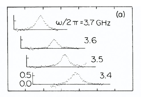
Figure 20: Experimental observations of SCD peaks for different frequencies of applied microwaves.

From this figure, peak positions can be extracted and plotted as functions of the microwave frequency (circles) – as shown in Fig.21. This has been done as well for two of the peaks in Fig. 2 of Martinis (squares) and, finally, (stars) for the two peaks in Fig. 3 of Berkley (see Blackburn1 ; Blackburn2 ).

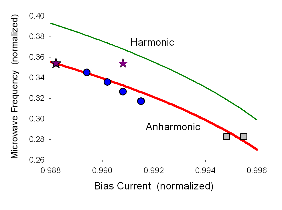
Figure 21: Summary of experimental results from two groups on observed SCD peak positions - circles and squares Martinis , and stars Berkley .  Continuous curves were generated from expressions for harmonic and anharmonic resonances.

Clearly, the positions of these various experimentally observed peaks closely match the expectations of anharmonic resonances in the washboard potential well – a prediction of the RCSJ model. In the case of two peaks seen by Berkley et al. Berkley at $5.7\,GHz$ the one located at a higher bias is close to the harmonic approximation for a resonance at this frequency.

Thrailkill et al. (2012)

As an example, we consider an experiment by Thrailkill et al. Thrailkill . In this experiment, the bias current was swept in the presence of microwaves of specified frequency. The parameters of the junction were: $I_{C}=9.485\mu A$ and $C=4.7pF$; the Josephson plasma frequency was thus $f_{J0}=12.46GHz$. For the simulation Blackburn1 , the Lorentzian response to the applied microwaves was specified by $a=0.09$ and $b=0.003$. The values of the normalized bias values at resonance ($\eta_{res}$) for each of the experimental microwave frequencies were $0.972,\,\;0.976,\,\,0.980,\;0.984$ respectively. As shown in figure 22, the RCSJ simulation replicates the experimental observations even in a situation where the microwave-off peak (thermal activation) is quite close to the microwave-on peak (ac activation).

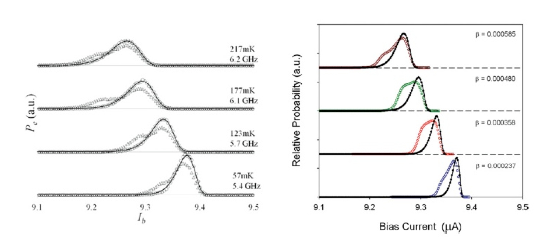
Figure 22: Left: Experimental results for SCD peaks with (circles) and without (solid) applied microwaves. Right: RCSJ simulation with parameters corresponding to the experiment.

Wallraff et al. (2003)

Wallraff et al. Wallraff2 revisited the swept bias type of experiment pioneered in the works, almost two decades earlier, discussed in the section: Martinis et al. (1985). As in those earlier experiments the procedure was simple: microwaves at a given frequency were applied and repeated bias scans were carried out to accumulate data for a switching current distribution. The results are shown in Fig.23.

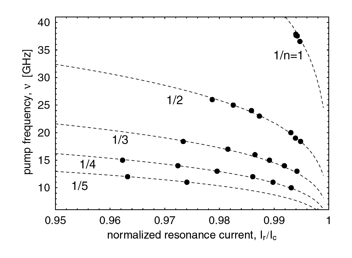
Figure 23: Applied microwave frequency $\nu$ versus normalized resonant bias bias current $I_{r}/I_{C}$.

Each dot is an experimental data point. Twenty frequencies in the range $10.113$ - $37.894\;GHz$ were employed,  Most were single peaks for a given frequency, but four of these ($13.111,14.095,15.126,18.499$) yielded twin SCD peaks separated by slightly different bias values. These experiments showed clearly that the SCD peaks were located at bias currents for which the frequency of the applied microwave signal was matched either to the fundamental or to submultiple values of the expected resonance frequency determined by that bias current according to the expression $\nu=\left(1/n\right)\nu_{P}\left[1-\left(I_{r}/I_{c}\right)^{2}\right]^{1/4}$, $n=1,2,3..,$ where $I_{r}$ is the bias current at the SCD peak and $\nu_{p}=116\;GHz$.

The frequency spacing of the quantum levels was supposed to be tuned according to the dependence of the plasma frequency upon the external dc bias current. It was claimed that single photon and multiphoton transitions between junction energy levels had been observed.

However, Grønbech-Jensen et al. (next section) reconsidered the conclusions to be drawn from this experiment.

Grønbech-Jensen et al (2004)

Shortly after the publication of the results of Wallraff et al. Wallraff2 , the collaboration of Grønbech-Jensen et al. NGJ1 reported an extensive investigation of the response of Josephson junctions under the influence of external microwave signals in the range $350mK<T<1.5K$ . This work showed that all the excitations in the “escape” measurement spectrum could be explained, within the RCSJ model, essentially by Eq.26 including a noise current term; the analysis also showed striking agreement with analytical predictions based on the interaction of the external signal with the bias current-dependent Josephson plasma resonance. These measurements confirmed the correctness of the data presented by Wallraff et al. Wallraff2 . In particular, Fig. 24 (Fig.3 from NGJ1 ) shows the underlying harmonic features of the SCD phenomenon.

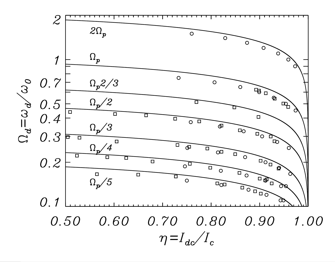
Figure 24: Positions of peaks in switching current distributions as functions of subharmonic and harmonic pumping. Circles represent numerical results and squares experimental data.

Because numerical simulations were in excellent agreement with the results from Wallraff2 , this clearly showed that the excitation spectrum belonged to the realm of classical Josephson phenomenology. It was also shown that the contribution of the anharmonicity of the potential well to the spectrum was relevant NGJ2 and an excellent agreement between data and anharmonic plasma resonance approximation was reported, as shown in Fig 4 of NGJ1 . Most importantly, it was found that no substantial differences exist in the response of the junctions from $1.5K$ down to $360mK$. The latter value was slightly above the crossover temperature of the junctions (estimated to be $320mK$). When comparing the measurements of Refs. NGJ1 ; NGJ2 on the ac response of the junctions with the similar ones collected at temperatures safely below the crossover Wallraff2 one realizes the complete similarity of the data and it is hard to conjecture traces of temperature-induced discontinuities or abrupt gradients in the response of the junctions for temperatures above, close, and below the crossover value: this is in reality a further argument in favor of the conclusion already expressed, that there is not much room to speculate on the existence of a crossover temperature and a consequent transition to an MQT regime.

In the conclusion of NGJ1 , the authors state: “The experiments reported in Wallraff2 have produced ac-induced peaks in the observed switching distributions, and the relevant peaks are located alongside the expected classical plasma resonance curve, as we have also found here. An important observation is that the microwave radiation frequency necessary for populating an excited quantum level ($\hbar\omega_{d}$) in a quantum oscillator coincides with the classical resonance frequency of the corresponding classical oscillator. It is evident then that multipeaked effects are not a unique signature of quantum behavior in the ac-driven Josephson junction.”  The last sentence is significant in that the RCSJ was confirmed as a complete discriptor of the experiment.

Silvestrini et al.(1997)

An interesting experiment claiming the observation of quantized energy levels of the washboard potential, in the absence of applied microwave radiation, was reported in 1997 by P. Silvestrini et al..Silve97 The idea of this experiment was to evidence quantum levels through a very fast ramp of the current biasing the junctions. The physics at the basis of the experiment was that it should be easier to observe possible quantized levels of the potential wells when a fast ramping out of these generates non stationary conditions which do not give the possibility to the junctions to thermalize. In principle, the experiments could be performed even above the crossover temperature and in fact the measurements were performed in the range $1.5K-4.2K$. This idea had a significant impact on the community because the results, see Fig.25,

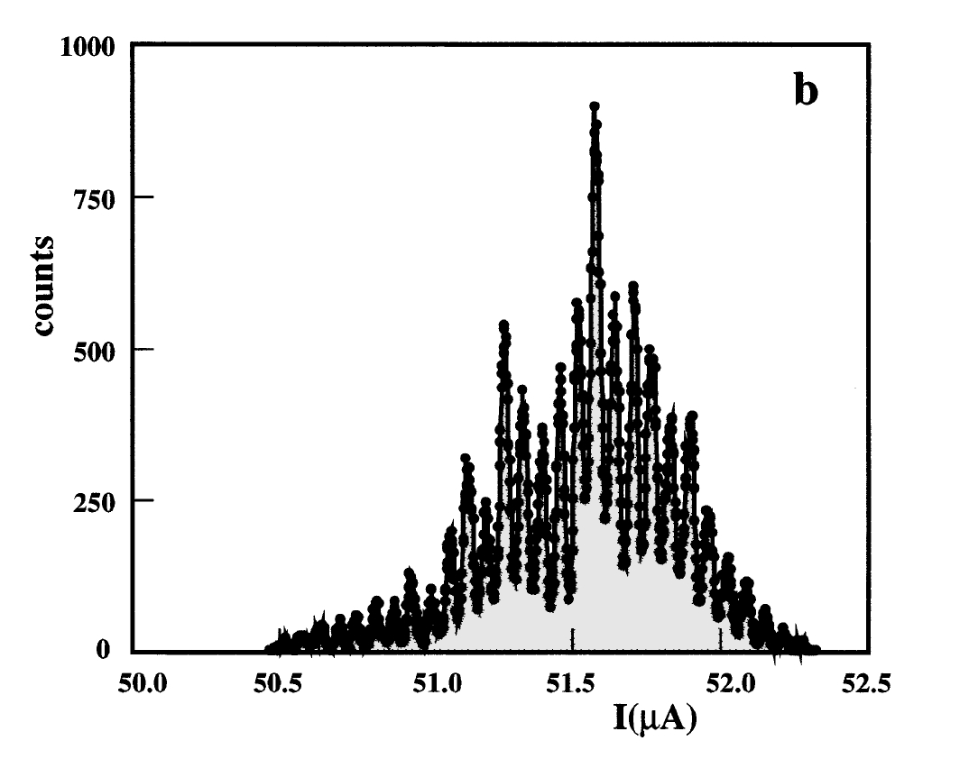
Figure 25: Figure 2 b from Silve97 showing experimental switching current distribution at high sweep rate.

appeared to represent an independent proof of the existence of the quantized levels previously claimed by the microwave spectroscopy experiments.

We know now that the microwave spectroscopy experiments of the 80’s can be well accounted for by RCSJ model physics, and so a claim of unambiguous evidence of quantized levels should be based exclusively on the results of the Silvestrini 1997 experiment. Such a claim would also be questionable since we have observed several times, both in small area and large area junctions RCSJ simulations, that a very fast bias current ramp can generate, in thermal escape histograms, effects that look like the “levels” reported by Silvestrini et al. Silve97 . In Fig.26 from NGJ6 one can see a typical example of the dependence of escape histograms upon the sweep rate: a multi levels-like histogram can be seen in this specific case for $10^{-5}<\frac{d}{dt}\eta_{dc}<10^{-4}$

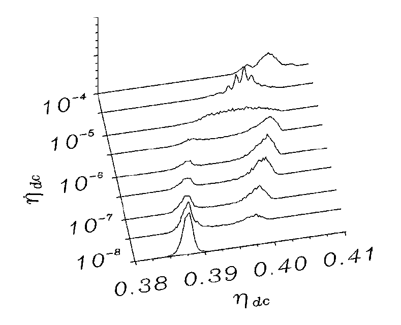
Figure 26: Simulated switching distributions at different sweep rates ($\dot{\eta}_{dc}=10^{-8}\rightarrow 10^{-4}$).

For high sweep rates one can obtain features very similar to those of Fig.LABEL:SilvestriniFig2; moreover, we have observed that the ”levels” exhibited in the RCSJ model at fast sweeps also disappear with increasing losses or temperature. Thus, even in the case of the experiments of Silvestrini et al.Silve97 the observed effects cannot be uniquely attributed to quantum modelling. The sweep rate is a relevant parameter as far as escape from potential wells is concerned and its relation with the statistical output of the experiments/simulations must be evaluated very carefully.

IV.4 Annular Junctions

The preceding sections have considered phase dynamics in small Josephson junctions, namely junctions whose spatial dimensions are small with respect to the Josephson penetration depth $\lambda_{j}=\sqrt{\frac{\Phi_{0}}{2\pi\mu_{0}dJ_{c}}}$ (here $\mu_{0}=4\pi 10^{-7}H/m$ , $d$ the magnetic thickness of the junction and $J_{c}$ is the Josephson maximum super current density). We now turn our attention to another, closely related, system - an annular Josephson junction- namely a junctions for which the superconducting electrodes overlap along a circle. In this case we have just one spatial degree of freedom for the phase if the length of the circle is larger than $\lambda_{j}$ while the overlapping region is smaller than $\lambda_{j}$; it is known that this degree of freedom, even just in a one-dimensional configuration, gives rise to the presence of Josephson flux-quanta (fluxons) along the spatially extended dimension, i.e., along the circular path Davidson1986 ; Ustinov ; Martucciello ; an annular junction is depicted in Fig.27 Wallraff .

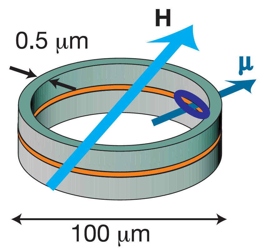
Figure 27: Schematic diagram of an annular Josephson junction. Superconducting electrodes (not shown) connect to the upper and lower portions of the junction. H is an externally applied magnetic field and $\mathbf{\mu}$ indicates the magnetic moment of a single trapped fluxon.

where we can see ring-shaped upper and lower superconductors separated by an oxide barrier. The complete device can be visualized as the overlap junction shown in Fig.28

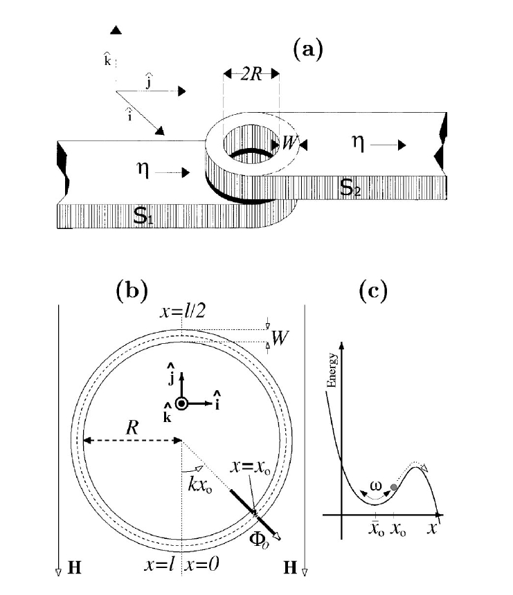
Figure 28: Fig. 1 from NGJ6 showing a complete annular junction.(a) and the potential energy as a function of the vortex coordinate.

with a hole drilled through the overlapping fingers as indicated in Fig. 28. Bias current is sent in to and out from the junction via superconducting films.

The experiments of Wallraff et al. Wallraff observed the motion of a single trapped fluxon in the plane of the annular junction - depicted as a vector labelled $\mathbf{\mu}$ in the figure. The technique for trapping a single fluxon in the ring is discribed in Ustinov : “trapping of a magnetic flux in the junction ring was made while cooling the sample below the critical temperature $T_{C}=9.2$ $K$ of niobium”. As noted in Martucciello et al. Martucciello , about $10$ or $20$ attempts could be necessary before a single fluxon was trapped this way.

A fixed external magnetic field $\mathbf{H}$ is applied in the plane of the junction; this sets the preferred minimum energy orientation of the fluxon, just as gravity does for a free hanging pendulum. A steady bias current passes vertically through the annular junction as a ring shaped sheet.  Since the fluxon axis is always radially directed, the Lorentz force on the fluxon is always tangent to the ring, and is constant. This is analogous to a steady torque on a pendulum. Whereas a pendulum has a critical torque ($mg\ell$) beyond which rotational motion occurs, the annular junction will have a critical bias current above which the fluxon will circulate around the ring.  When that happens, a voltage will appear across the junction.

The dynamics of this system are described in NGJ6 .

$$\varphi_{tt}-\varphi_{xx}+\sin\varphi=\eta_{dc}+\eta_{ac}\sin\omega_{d}t+\Gamma k\sin kx-\alpha\varphi_{t}+n(x,t)$$ (30)

where $\varphi(x,t)$ is the order parameter phase difference across the junction and $x$ is the fluxon coordinate measured around the circumference of the ring. This is a sine-Gordon equation with dissipation $\alpha$, a forcing term due to an applied magnetic field $\Gamma$ and, finally, thermal noise $n(x,t)$.

Experiment with Microwaves OFF

As with a  simple Josephson junction, the point at which the switch from static (zero voltage) to dynamic (nonzero voltage) occurs depends on the presence of any additional noise and, in these experiments, this is thermal noise. Noise causes the switching to happen just before the critical bias is reached, but with statistical likelihoods. As with the simple Josephson junction, repeated bias sweeps produce distributions in the switching moment (see Fig.9). The temperature dependence of this escape process is evident from Fig.29.

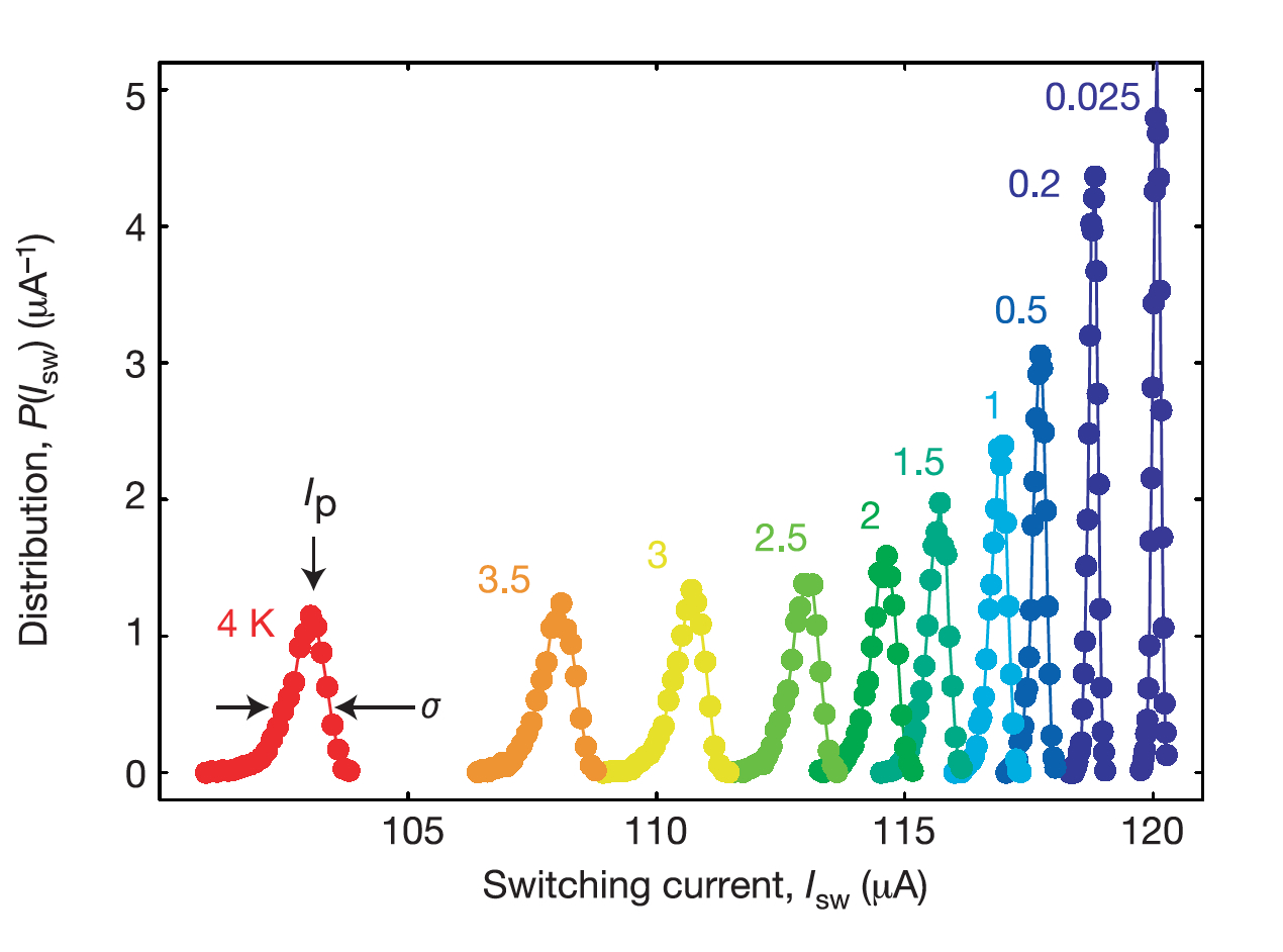
Figure 29: Probability distributions for escape to a running fluxon state in an annular Josephson junction Wallraff .

The peaks in the swept bias escape distributions clearly have the same attributes as the corresponding data for a small area Josephson junction (Figs.9 and 11).

As is commonly done, peak widths were chosen for close scrutiny and presented on a log-log plot (Wallraff , Fig.30). There does appear to be a suggestion of saturation of the widths at the lowest lowest temperatures, but as discussed in III A, the log-log treatment gives a visual appearance of flattening that may be deceiving.

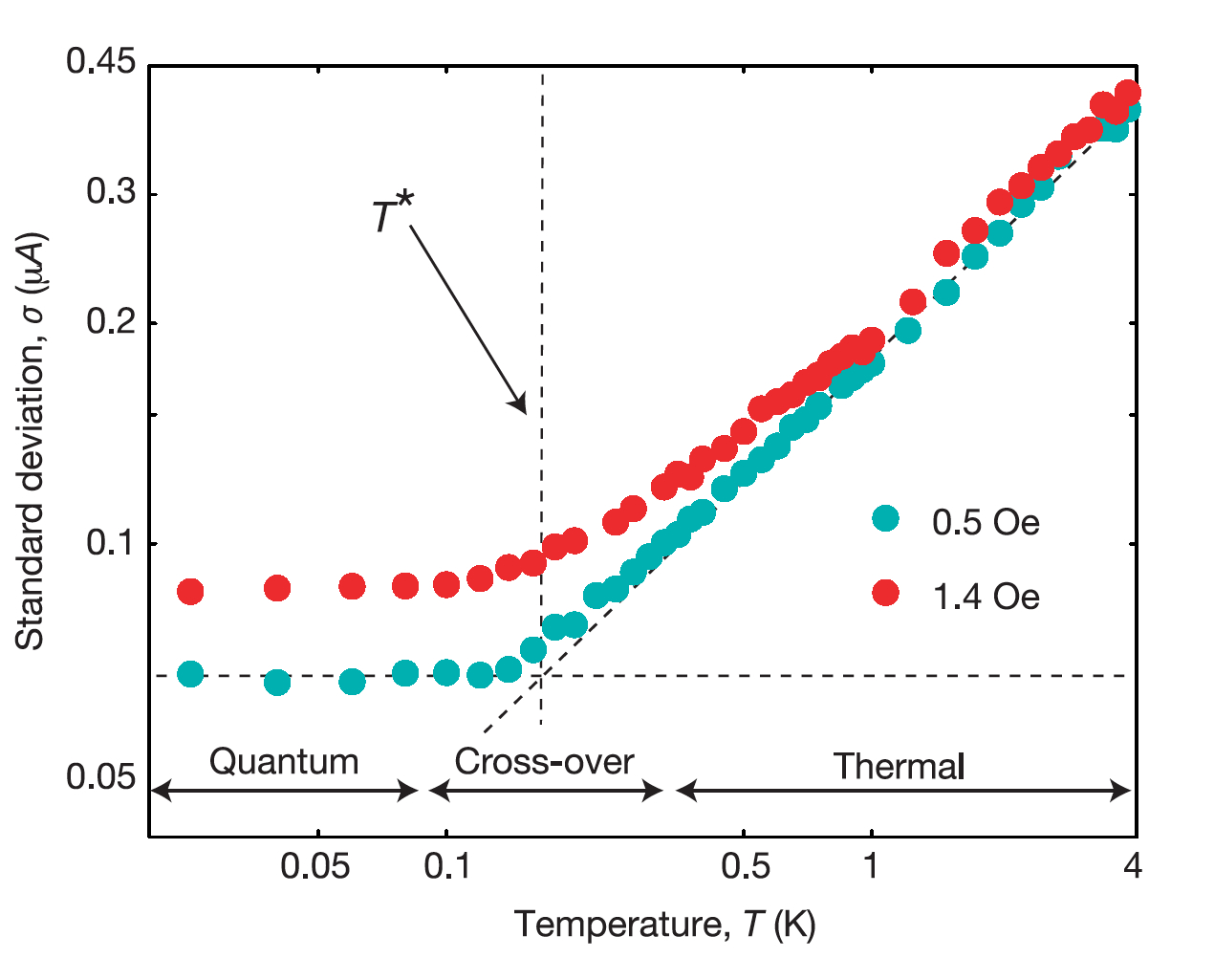
Figure 30: Figure 2 from Wallraff showing the SCD escape peak widths as a function of temperature.

For example, the same data in this figure can be replotted with conventional linear scales, as is done in Fig.31.

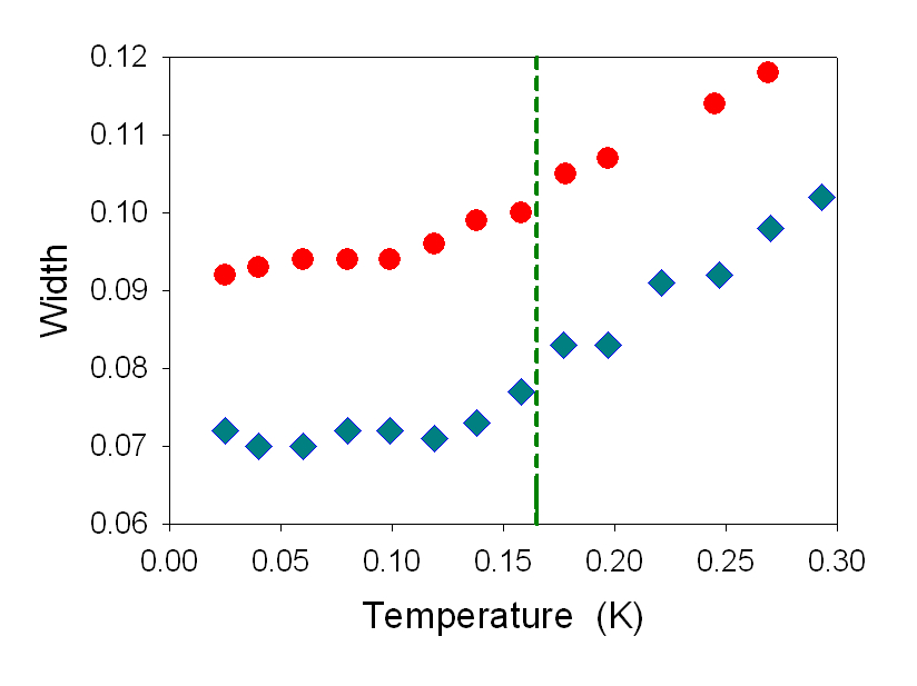
Figure 31: Data from Wallraff , Fig 2b plotted with linear scales. The dashed line indicates the postulated crossover temperature.

Now the trends appear gradual, without any dramatic flattening below the purported crossover temperature. However, peak widths are quite small at the lowest temperatures and their precision is much less than peak position data.

More revealing is the behavior of peak positions. As with the data of Voss and Webb VossWebb and Yu et al. Yu , escape peaks reported by Wallraff et al. (Wallraff Fig. 29) are seen to advance steadily as the temperature is lowered, and this continues well below the anticipated crossover temperature. It is clear in Fig.32 that this trend does not exhibit any sign of becoming temperature-independent as would be expected if there were a transition to MQT where the escape rate itself would be temperature independent. (It would be helpful if many more data points were recorded to fill in this plot below $500$ mK)

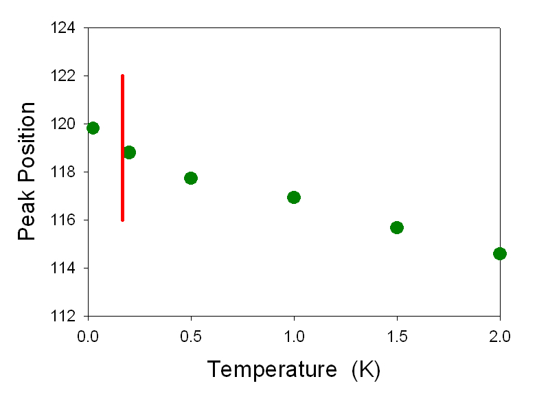
Figure 32: Peak positions from Wallraff as functions of the bath temperature.  The vertical line indicates the reported crossover temperature. Note the absense of peak ‘freezing’ at the lowest temperatures.

This alone calls into question any claim that a condition of temperature-independence has been reached at the lowest temperatures of the experiment.

The trend in these experimental widths is unconvincing, and the trend in the experimental positions decidedly disagrees with quantum expectations.

 Experiment with Microwaves ON

The focus of experiments on annular junctions has been the effects of applied microwaves. From a classical phenomenological perspective, it would be anticipated that resonant activation would occur when the microwave frequency matched the natural frequency of a fluxon at a given bias condition.

The experimental results from Wallraff are shown in Fig.33.

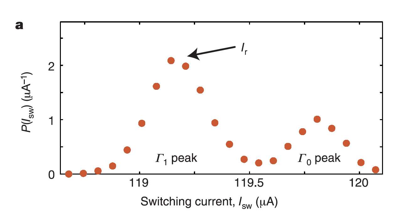
Figure 33: SCD escape peaks with $11$ GHz applied microwaves at $T=25$ mK.(Fig.3a from Wallraff ).

According to Wallraff et al.: “The peak at higher bias current is due to the tunnelling of the vortex from the ground state, whereas the peak at lower bias current corresponds to the tunnelling out of the first excited state”. In other words, the $\Gamma_{0}$ peak is present with or without microwaves whereas the $\Gamma_{1}$ peak is observed additionally when $11$ GHz microwaves are present. The peaks are at switching currents of $\ \Gamma_{0}=119.79\mu$A and $\Gamma_{1}=119.09\mu$A; $\ \Gamma_{0}$ is the same as the $25$ mK peak in Fig.29.  Note the similarity of this two-peak plot to the data of Thrailkill et al. Thrailkill shown in Fig.22 where one peak is microwave induced and the other is simple thermal activation.

Numerical simulations based on Eq.30 yield results such as depicted in Fig.34.

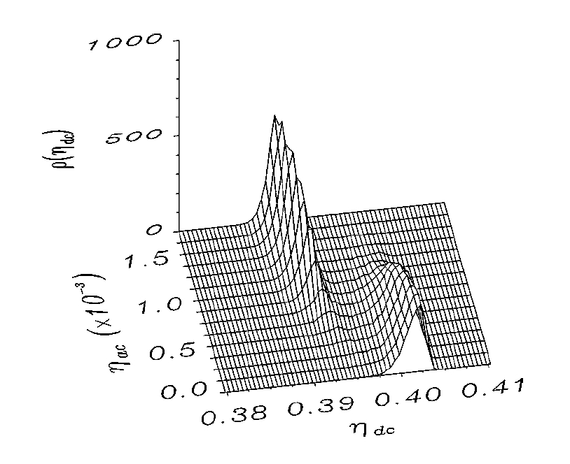
Figure 34: Simulation results for an annular Josephson junction NGJ6 .  For each possible choice of ac drive amplitude, the vertical axis indicates the relative probability that the junction will switch to a finite voltage state (circulating fluxon) as a function of dc bias.

With no excitation $\eta_{ac}=0$, there is a single escape peak. It is also evident that there is a range of excitation amplitude $\eta_{ac}$ for which there are two SCD peaks, the upper one that occurs even without excitation and a second peak at a lower $\eta_{dc}$ dc current.  For $\eta_{ac}\simeq 0.8$ this double peak structure approximately matches the experimental result shown in Fig.33 and confirms the adequacy of the classical RCSJ model in capturing the system behavior.

V Artificial Atom Analogies

V.1 Rabi Oscillations

At the end of the 90’s a general belief existed that robust evidences of new macroscopic quantum coherence effects in Josephson systems had been achieved (indeed unambiguous evidences were already claimed at the end of the 80’s Leggett87 ). Along with the fact that in the mid-90’s two theoretical algorithms showed the powerful possibilities offered by systems operating in a controllable quantum superposition state Shor ; Grover the above evidences generated a noticeable squeezing of intellectual resources toward experiments which could demonstrate possibility of manipulation of the Josephson quantum states. In 2002 John M. Martinis and his group in Boulder MART2 , relying on the fact that a Josephson junction could behave as system with quantized energy levels, presented results in which the physics predicted for a two levels quantum systems could be expected from a Josephson junction and its washboard potential. The physics of the fundamental process was dating back to the arguments presented by Isaac Rabi in 1937 Rabi37 who considered a multilevel atomic system. Rabi oscillations have been also considered within the context of quantum optics Loudon .

The application of external microwaves of adequate frequency to the atom (the atom being the Josephson junction) for a given time would generate a flipping between energy levels which, in turn, could give rise to oscillations in the population of the energy levels, known as Rabi oscillations. The status of the system (i.e., the level population) was investigated by a technique employing a sequence of pump pulses and probe pulses. Both pump pulse and probe pulse consisted of a small amplitude microwave signals applied to the junctions for given times: the pump pulse was responsible for the flipping between levels while the probe pulse was responsible for testing the final population in the states by potential escape techniques.

The evidence of Rabi oscillationsMART2 , namely the oscillations in the population of the first excited level as a function of the applied microwave power was striking and therefore this experiment was considered a conclusive evidence of the possibility that Josephson junctions could behave as elementary bits of quantum information, or qubits. Indeed, from that time on a new terminology took over when referring to Josephson circuits: in particular, circuits relying on single tunnel junctions for quantum operation were baptized “phase qubits” while circuits employing macroscopic quantum flux states (like rf-SQUIDSs and dc-SQUIDs) “flux qubits”. Beside the fashionable names it is worth recalling these were just Josephson junctions devices. The application of microwave pulses of suitable frequency and duration to an atom could increase the population of an upper state. In the Rabi effect the degree of population enhancement is a periodic function of the amplitude of the pump pulse. The status of the system (i. e., the level population) can be investigated by means of a probe pulse. Both pump pulse and probe pulse consist of a small amplitude microwave signals applied for given times.  The experiments of Martinis et al. MART2 were predicated on the supposition that a Josephson junction at temperatures around $50$ $mK$ would have entered a macroscopic quantum state, and thus could be viewed as an artificial atom.  Therefore, phenomena like Rabi oscillations ought to be observable.

The experimental evidence for Rabi oscillations presented in MART2 (see the upper panel of Fig.35)

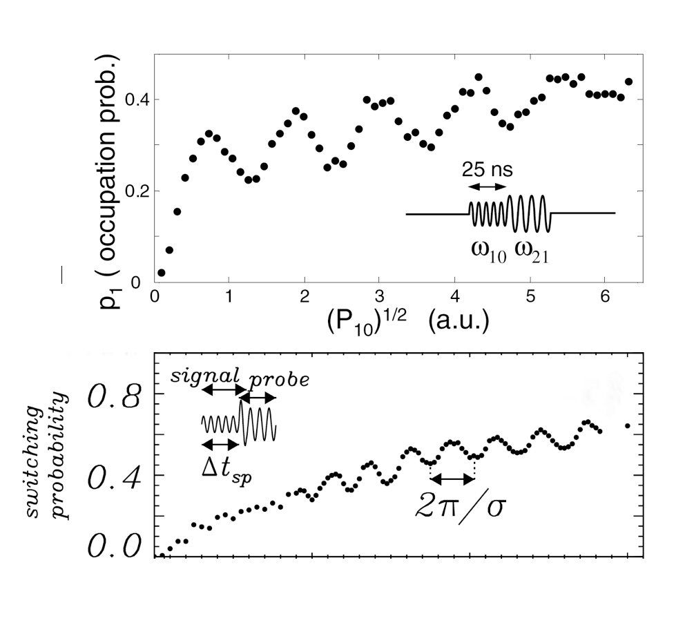
Figure 35: Rabi oscillations: upper panel, experimental results reported in MART2 .  The probability is plotted as a function of the microwave pulse amplitude; lower panel, simulation based on classical junction description NGJ4 .

seemed persuasive and this added to the consensus in the MQT community that a Josephson junction would indeed function as a qubit at very low temperatures.

During the first half of the 2000-2010 decade, however, numerical techniques for simulating escape processes in Josephson junction through the RCSJ model had been set up and calibrated in a number of papers Kautz ; NGJ0 . The numerical simulations had shown striking agreement with experimental reality and analytical approaches for ac driven junctions. Thus, three years after the appearance of Martinis and co-workers’ paper on the Rabi oscillations, papers were published NGJ3 ; NGJ4 in which it was shown that the features reported in the Martinis Rabi paper could be well interpreted by the nonlinear phenomenology of Josephson junctions. The analytical approximations were in striking agreement with numerical simulations and the experimental results MART2 ; Claud1 as revealed in the lower panel of Fig.35, and by the comparison between analytical ansatz, numerical simulation and experiments shown in  Fig.36.

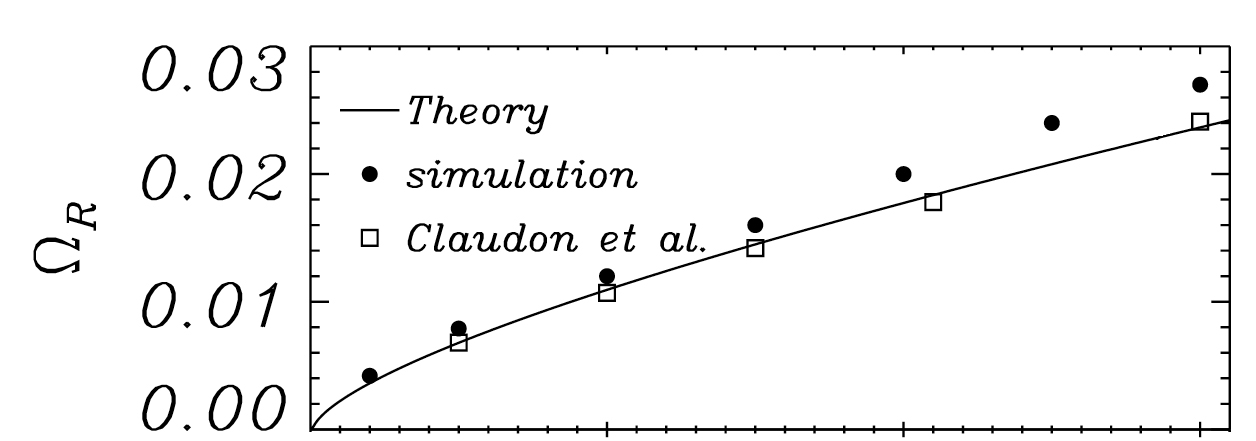
Figure 36: Modulation frequency $\Omega_{R}$ as a function of microwave amplitude $\epsilon_{S}$ (horizontal scale $\epsilon_{S}:0\rightarrow 0.003$).

The basis for the “classical” explanation of Rabi-like oscillations in Josephson junctions was a phase-locking ansatz (between junction internal oscillations and microwave signal) and a perturbation analysis of the phase-locked states introducing a transient modulation whose frequency could capture all the observed experimental features.

V.2 Ramsey fringes and Spin echoes

Following the paper by Martinis et al. in 2002 other publications appeared EstDev ; PLOURDE05 in which the experimental “microwave pulses” protocol was extended to reproduce other features (mostly coming from analogies with NMR research techniques) of the Josephson artificial atom like the observation of Ramsey fringes Ramsey50 and spin echoes Hahn50 . However, it was soon demonstrated that even these features could be explained as consequences of the RCSJ model of Josephson systems. Both Ramsey fringes JEFF1 and spin echo oscillations were reproduced for a single junction system JEFF2 and for SQUIDs JEFF3 . Ramsey fringes and spin echo–like effects could be activated in Josephson junction systems by appropriate combined sequences of pumping and probe pulses. These combinations can mimic accurately what were attributed to rotations on the Bloch sphereEstDev : A synthetic scheme for the generation of Rabi oscillation, Ramsey fringes and spin echo are shown in Fig. 37 (Fig.4 of JEFF3 ).

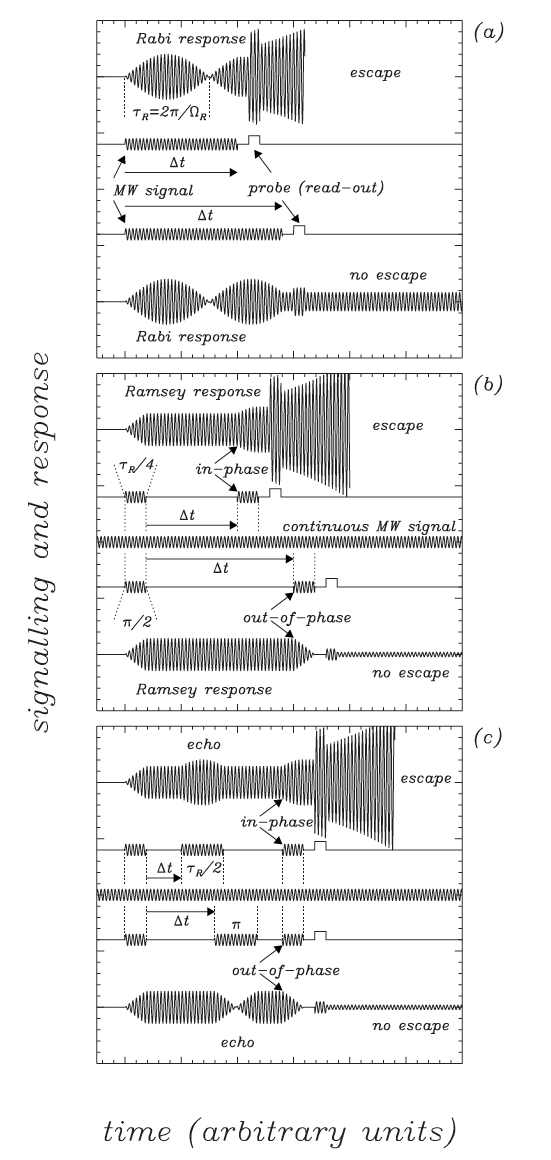
Figure 37: Figure 4 from JEFF3 .

In Fig. 38 (Fig 4 from PLOURDE05 )  we show Rabi oscillations and Ramsey fringes measured on a SQUID system investigated from the “quantum” point of view,

Figure 38: Figure 4 from PLOURDE05 .

(Fig.5 from JEFF3 )

Figure 39: Figure 5 from JEFF3 .

we show results of RCSJ simulations of the same system. As can be seen in these cases, like in all the others already discussed, the agreement of the RCSJ output with the experiments is remarkable.

The experiment described in MART2 was framed by the idea that the washboard potential for a Josephson junction would become quantized at very low temperatures and therefore, having thus become an artificial atom, it should exhibit phenomena such as Rabi oscillations.  The very names “pump” and “probe” in speaking of the weak microwave bursts convey the expectation of what would be occurring in the experiment - that some of the occupants of a lower state of the artificial atom would be pumped up to a higher state by a microwave pulse, and that the altered occupancy of the higher level could be sensed with a second probe pulse.

Oscillations that look like Rabi oscillations may indeed spring from another type of physics and thus do not constitute proof that anything quantum is going on.

VI Coupled Junctions

If superconducting qubits are to be exploited for quantum computing, it needs to be possible to produce entangled states. To this end, experiments were devised (Steffen ) in which a pair of qubits, macroscopically coupled by a circuit element – a capacitor – were subjected to a sequence of microwave bursts and pulses intended to condition and examine the state of the qubits. Our approach to a description of this experiment is strictly from the point of view of the RCSJ junction model. Steffen et al. Steffen provided the schematic shown in Fig.40 as an equivalent circuit for their coupled experimental qubits.

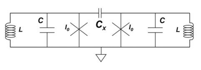
Figure 40: Diagram from Steffen representing the equivalent circuit of the experimental system.

For this treatment, we express this schematic as shown in Fig.41.

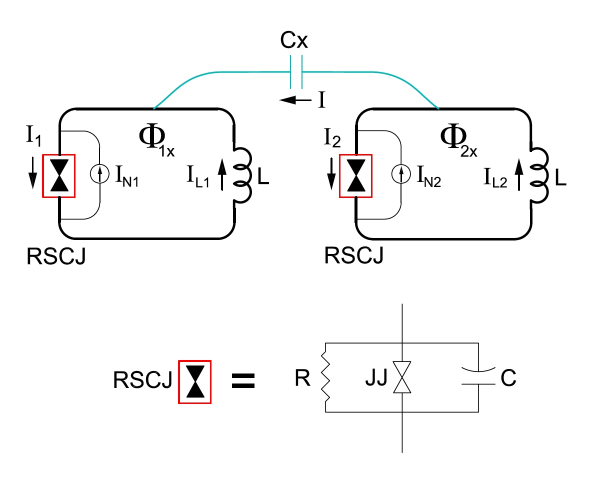
Figure 41: Equivalent circuit used in the RCSJ simulations.

As indicated, each junction is represented by its RCSJ equivalent: the parallel combination of a critical current $I_{C}$, a resistance $R$ , and a capacitance $C$. Each loop in the experimental sample has an associated inductance $L$. $\Phi_{1x}$ is an external flux applied to loop #$1$; $\Phi_{2x}$ is applied to loop #$2$.

The phase dynamics for the two junctions depicted in Fig.41 are governed by the following equations.

$${\ddot{\varphi}_{1}+\alpha\dot{\varphi}_{1}+\sin\varphi_{1}} {=\gamma_{X}\left(\ddot{\varphi}_{2}-\ddot{\varphi}_{1}\right)-\beta_{L}^{-1}\left(\varphi_{1}+2\pi M_{1x}\right)}$$ (31)

$${\ddot{\varphi}_{2}+\alpha\dot{\varphi}_{2}+\sin\varphi_{2}} {=\gamma_{X}\left(\ddot{\varphi}_{1}-\ddot{\varphi}_{2}\right)-\beta_{L}^{-1}\left(\varphi_{2}+2\pi M_{2x}\right)}$$ (32)

where overdots denote derivatives in dimensionless time $\tau=\omega_{J}t$ and with each of the junction plasma frequencies being $\omega_{J}=\sqrt{2eI_{C}/\hbar C}$. The parameters were $\alpha=1/\omega_{J}RC$ and as before $\beta_{L}=2\pi LI_{C}/\Phi_{0}$ with $\Phi_{0}$ being the flux quantum. The two external fluxes appear in$M_{ix}=\Phi_{ix}/\Phi_{0},\;\;\;i=1,2$ with the mutual coupling coefficient $\gamma_{X}=C_{x}/C$, $C_{x}$ is the macroscopic coupling capacitor, as shown in the figure.

Based on published experimental data Steffen , we set the parameters at: $\alpha=5\times 10^{-5}$ (very light damping), $\beta_{L}=2.841,\;\gamma_{X}=0.00231,\;I_{C}=1.1\mu A,\;C=1.3pF$, and $\omega_{J}^{-1}=0.02ns$ (plasma period $12.6ns$). The critical applied flux was thus $\Phi_{xc}=0.7022$; both loops were biased with a normalized dc flux $\Phi_{x}=0.6941$. Stimulus signals were added to the flux bias on one of the loops as indicated in Fig.42, which also displays the results of a numerical solution Blackburn4 of the coupled differential equations. The duration of the microwave burst was set to $100$ plasma periods; the amplitude and normalized frequency were $0.000580$ and $0.989$, respectively. A rotation pulse of amplitude $0.000915$ was applied at time $9550$; its duration in each of the three panels was $0,\;60,$ and $120$ plasma periods, corresponding to $0,\;7.5,$ and $15$ ns.

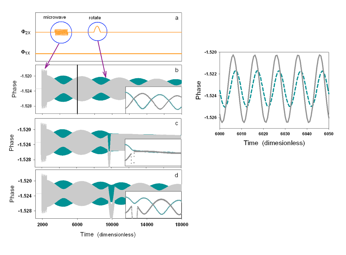
Figure 42: Left: RCSJ simulation results for coupled loops. The external bias flux for each loop is depicted in panel a. Panels b,c,d show the result of the applicationof a rotate pulse of varying duration - 0, 60, and 120 plasma periods; Right: Phase oscillationsexpanded around the vertical line in panel b of the figure on the left.

This is a case of two coupled oscillators, one of which is kick-started with an applied signal, after which there is a back and forth exchange of energy. This is entirely analogous to the case of two weakly coupled pendulums – a standard topic in classical mechanics Chow . In that situation the pendulum oscillations exhibit low frequency envelopes. The undulations of the junction phases depicted in the three lower panels in the figure on the left are composed of rapid excursions of the individual phases between their extremes (max and min); the close packing of the wave forms on that time scale results in the appearance of a solid color fill. The insets in these three panels show just the upper boundaries traced by the maxima of the junction phases. The figure on the right has an expanded time scale (around the vertical line in panel $b$) to reveal the uncompressed phase oscillations. The ratio of the envelope period to the junction oscillation period is more than $400:1$. In fact, as will be seen, it is this envelope that is probed by experiments.

To mimic the experiment, two additional elements must be added to the previous treatment. First, the finite sample temperature ($25mK$) needs to be included via the noise sources identified as $I_{N1}$ and $I_{N2}$ in the circuit schematic. Second, measurement pulses are required as indicated in this figure (43) taken from Steffen .

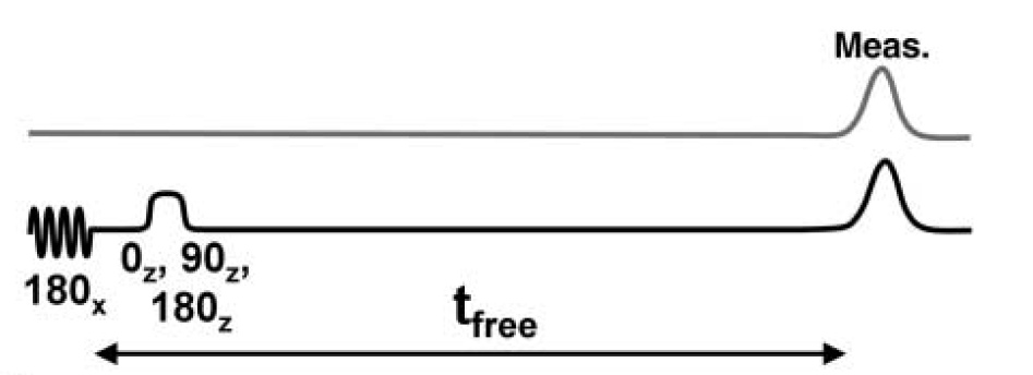
Figure 43: Bias pulse sequence as shown in Fig. (1) in Steffen .

To understand the action of a measurement pulse on either of the loops, consider Fig 44 which shows a close up view of the potential energy as a function of the net internal loop flux for an applied flux of $0.6941$ - just less than the critical value of $0.7022$. At this bias, the minimum in the potential well is located at $\Phi/\Phi_{0}=0.242$.

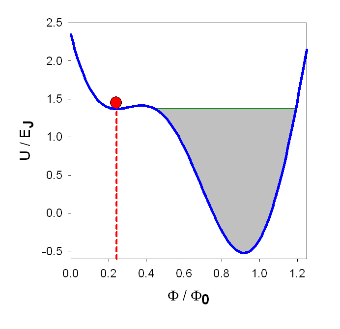
Figure 44: Energy-flux diagram for a bias close to the critical external flux.  If the ”particle” escapes from this shallow well, it will enter the much deeper well to the right and then oscillate around the new minimum.

The scenario goes as follows. Following the microwave pulse, the ‘particle’ in that loop is stimulated to oscillate at the bottom of its well. The amplitudes of those oscillations, as depicted in the previous section, are very small and centered around the minimum; they range from $0.2419<\Phi/\Phi_{0}<0.2430$ and are not discernable at the scale of this plot.

In our simulation Blackburn4 , a triangular measure pulse of amplitude $0.00358$ was applied at a set free time after the oscillations commenced; this is enough to briefly raise the applied flux to $0.6977$, closer to the critical value, allowing noise to pop the ‘particle’ over into the larger parabolic well indicated by shading in Fig.44. Oscillations that bring the ‘particle’ closest to the barrier just before the measure pulse stand the best chance of jumping out of the well with the aid of thermal noise. Escape to the deeper well and subsequent back and forth oscillations within it will be signalled by much larger phase oscillations and thus, voltage oscillations.

An individual simulation run produces one of two outcomes following the measure pulse: escape or non-escape. Repeated runs with the same time $t_{free}$ will yield a relative probability value for escape at that moment and that in turn is a measure of the magnitude of the phase oscillations – that is, the envelopes shown in the earlier figure.

The undriven but coupled loop will respond to the oscillations induced in the driven loop.

To match the experiment, the simulation was carried out as follows. For any chosen moment following the microwave burst, repeated simulation runs ($1000$ measurements) were carried out and data were gathered on how often there had been an escape in each loop as indicated by a jump in voltage following the measurement pulse.

The results of the RCSJ-based simulation are shown in Fig.45 together with the experimental data from Steffen .

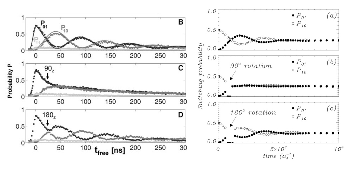
Figure 45: Left: Experimental observations as shown in Fig.2 of Steffen . Each panel is for a different rotation pulse; Right: RCSJ simulation results matching the corresponding panels on the left.

VI.1 Entanglement of Two Qubits

In Steffen the devices were described as “phase qubits”. However, as was pointed out in the earlier discussion, each Josephson junction was imbedded in a superconducting loop of inductance $850pH$ and so the energy consisted of a part due to the circulating supercurrent and a contribution from the Josephson coupling energy. Therefore in this situation these are flux qubits, not phase qubits. The loops are flux biased, not current biased. This is evident from Steffen Steffen Fig.1A where the “qubit bias” is inductively coupled into the qubit loop. This situation is distinctly different from the more common current-biased Josephson junction where the energy takes the form of a “washboard potential”. In the quantum picture for this system, it a fluxon that would escape from the well by tunneling out into the larger and deeper well.

We remark that the RCSJ model suggests that the action of the microwaves is merely to kick the ‘particle’ into oscillations within its shallow well, so in principle a brief plain pulse would work just as well. The MQT view is that microwaves are necessary to pump the ‘particle’ to a higher level in that initial well. So a significant test of this issue would be to substitute a simple pulse in both experiment and simulation. We would predict the experimental data would not be affected.

It is worth noting that in this case ”unambiguous” evidence of quantum behaviour of the coupled loops was claimed Steffen based on the fact that the density matrix had off-diagonal terms (see Fig.46) The belief was that a classical system could not possess such a property. That conjecture is naturally wrong if we think in terms of classical nonlinear systems, and indeed simulations of rf-SQUIDs coupled through a capacitor showed that a suitably defined density matrix could have off-diagonal terms NGJ5 . These simulations returned a picture very close to that obtained in the experiments, as shown in Fig.47. Bear in mind that Fig. 46 derives from experimental data while Fig. 47 is obtained from numerical simulation data from a fully classical model. Therefore state tomography cannot be considered a definitive test of quantumness in the source of the data.

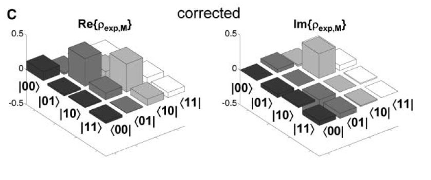
Figure 46: Figure 3c from Steffen showing state tomography applied to their experimental data.

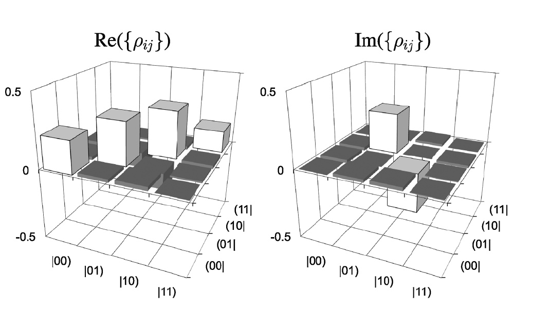
Figure 47: Results matching the previous figure, but obtained from purely classical data generated by the RCSJ model.

VII Historical Remarks

At first the idea of a classical/quantum transition became the subject of experiments by just a few groups, and the evidence did seem to be consistent with the macroscopic quantum hypothesis. Then the level of activity on the topic rose significantly. Josephson systems such as rf-SQUIDs, large area junctions, annular junctions, and configurations of coupled junctions were all examined with the expectation that they would provide confirmation at the lowest temperatures of the new quantum phenomenology, and most of the obtained results seemed to support that idea. By the early 90’s, in the absence of any detailed classical RCSJ simulations, it was was generally accepted within the community that the quantum hypothesis had been confirmed by experiments. Like supersolids Hallock , once the idea of a macroscopic quantum state was out there, people pursued it.

Unfortunately, several aspects concerning RCSJ simulations were not clear in the 80’s, mainly because computer simulations for the nonlinear circuit model, including dc and ac forcing currents, along with noise current terms, represented a rather challenging topic and few groups around the world having access to powerful computing facilities were able to tame it. Also, at that time, the exponential growth of the interest for chaotic dynamics moved the attention of the international community toward the intriguing and interesting evidences of chaos in Josephson systems Kautz1 and, more in general, toward spatio-temporal structures competition in nonlinear systems Christ1 . Thus, at the beginning of the 90ies, in the absence of specific and systematic RCSJ simulations, the existence of a crossover temperature, of energy levels in the Josephson potentials and their evidence through “spectroscopy” were generally accepted as a necessity.

The above historical conditions gave birth, at the beginning of the 90ies, to a research project MQCNY , aiming at securing evidence of Macroscopic Quantum Coherence (MQC was the acronym of the project) along the philosophy of a gedanken experiment proposed by Claudia Tesche TESCHE90 . The project was aiming to take advantage of the possible macroscopic quantum behaviour of Josephson circuits in order to provide proof of fundamental relations of quantum mechanics such as Bell’s inequalities. The experiment was based in particular on the double-well potential of an rf-SQUID, namely a superconducting loop interrupted by a Josephson junction. One well of the potential was supposed to be occupied by a current circulating clockwise while the other well was occupied by a current circulating counterclockwise. In principle, if the barrier between the two wells was sufficiently low, the net current in the rf-SQUID loop could be considered as being a superposition of the state of each well, and the system itself could be in a typical quantum singlet state. Using a dc-SQUID coupled to an rf-SQUID that served as a detector for the superposition state ,it should have been possible to probe the quantum properties of the superposition itself (see Fig.2 MQCNY ). The MQC experiment resulted in the development of a thermal escape technique necessary for probing tunnelling and potentialsKautz ; NGJ0 ; Barb .

At some point the basic circuit architecture of the MQC experiment was changed in order to introduce, following an idea of J. E. Lukens and co-workers LUPRB92 ; LUNA00 , a means of tuning of the height of the barrier separating the two wells of the rf-SQUID potential. A lower barrier could favor the interaction between the macroscopic quantum states in the two wells while the tunability could pinpoint the moment when the quantum interaction turned on. This tunability could be realized by replacing the single junction of the rf-SQUID loop with a two parallel junctions in a small subsidiary loop as shown in Fig.LABEL:tunablebarrier.

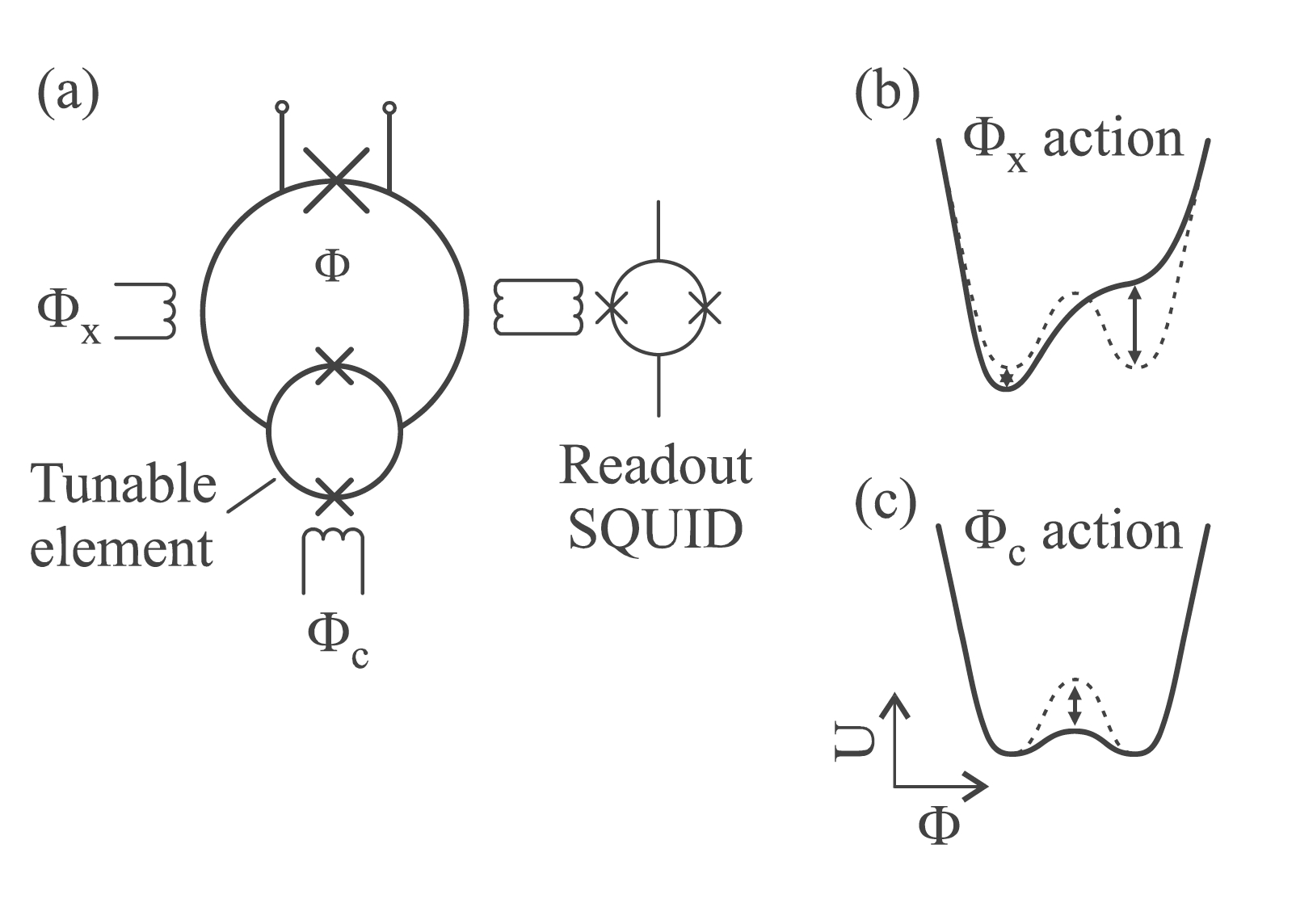
Figure 48: An rf squid containing a tunable element - two parallel junctions in a small sub- loop (dc squid).

Sophisticated and sensitive potential escape measuremets CATA07 at very low temperatures showed that the role of the inner loop giving rise to the tunability of the system modifies the shape of the potential giving rise to interesting features which can be explained within the general frame of the analysis of singularities in classical nonlinear systems Thom75 . It is most likely the nonlinear dynamic interaction between the junctions of the dc interferometer which originates a “gap” in the excitation spectrum which was interpreted as evidence of a quantum effect due to level quantization LUNA00 : in general indeed, we have found that a gap structure can arise in the excitation spectrum of two RCSJ oscillators whenever a coupling between those is allowed.

Over all, interactions between the two wells of the rf-SQUID potential expected in zero-applied microwaver (rf currents) have not been observed from escape measurements. Some interesting observations have been recently reported by pulsing the system with microwave burst Spilla14 , however, the discussion reported in the previous sections concerning the ”atom-like” responses of Josephson junctions indicates that collecting information by pumping withy external microwaves, or short microwave bursts, or anything else can hardly lead to unique “quantum” properties for Josephson systems . It must always be recalled that the junctions used for macroscopic quantum coherence experiments are of very good quality and, speaking in terms of RCSJ model, very lightly damped, and therefore a short burst of microwaves, or even just a single pulse, induces oscillations having a very long decay time which can allow modelling and manipulations even from a classical point of view.

VIII Recent Development

VIII.1 Qubits Coupled via Coax Cable

In the first publication reporting experimental results for coupled qubits Steffen , the coupling was provided by a macroscopic external capacitor. The interpretation placed on the experimental findings was entirely within a quantum narrative and concluded that entanglement had been observed. A classical equivalent circuit based on the RCSJ model led to a pair of coupled differential equations for the phase variables; numerical solutions of these equations Blackburn4 , NGJ5 were shown to fully replicate the experimental observations.  This cast significant doubt on the claims that quantum entanglement had been unambiguously demonstrated.

More recently, this kind of macroscopic coupling, now of two transmons, has been extended from a capacitor to a one-meter transmission line, as shown in Fig.49 from Roch .

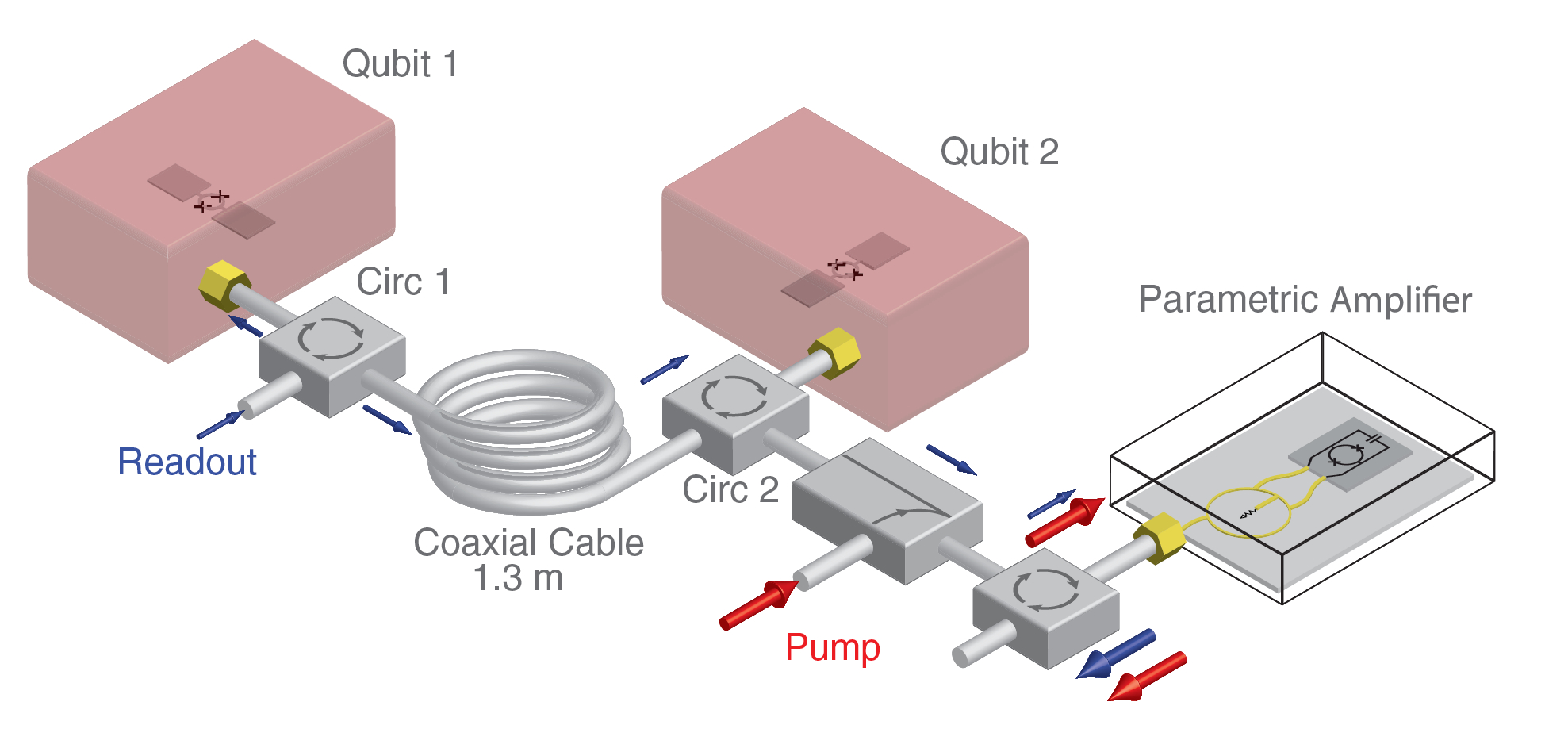
Figure 49: Depiction of coaxial cable coupling a pair of Josephson qubits.

A transmon is a particular configuration of Josephson junctions, as depicted in Fig. 50, taken from Koch (see also Krantz ).

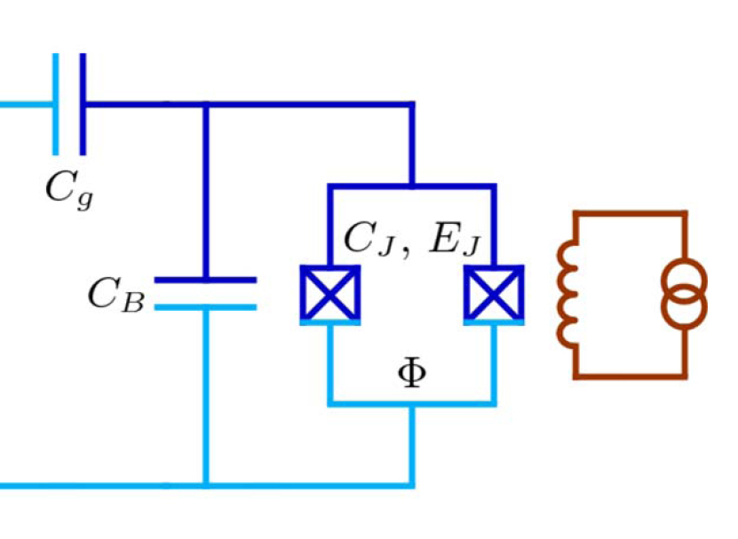
Figure 50: Equivalent circuit of a transmon qubit.  Each crossed-box is an RCSJ Josephson junction. The loop is flux biased by the subcircuit to the right.

IX Final Comments

All of the experiments reviewed here were intended either to confirm the existence of a macroscopic quantum state for Josephson junctions at very low temperatures, or to exploit the anticipated properties of a junction in the macroscopic quantum state. The simplest and most straightforword investigations were structured as swept-bias experiments, both with and without applied microwaves. These experiments recorded the value of the bias current at the moment when a finite voltage suddenly appeared across the junction.  Accumulated data from repeated bias scans provided switching current distributions (SCD). Without microwaves, a single SCD peak is seen. MQT theory predicted that the position of this peak should become temperature independent at sufficiently low temperatures. Such peak freezing is a sine qua non of any claims that a macroscopic quantum state has been achieved. As shown in this review, close inspection of experimental data clearly indicates that peak freezing has not been seen.

When microwaves are present, additional SCD peaks appear, commonly just one or two. These are well described as resulting from classical resonant activation at the anharmonic, or harmonic, plasma frequency. What has not been reported are multiple peaks expected from different pairs of inter-level spacings in a well.

Next were experiments involving more complex superconducting circuits; they were focused on expectations arising from the artificial atom picture of a low temperature Josephson junction. Finally, there were experiments consisting of a coupled pair of superconducting loops, each containing a Josephson junction.  These were intended to probe anticipated quantum entanglement.

It is worth recalling that above a hypothetical transition temperature, circuits containing Josephson junctions can be fully modelled with classical components (capacitors, inductors, resistors) together with the Johnson-McCumber-Stewart Josephson junction model from 1968.  The key question is whether a transition to a macroscopic quantum state occurs at sufficiently low temperatures. At present the allure of a superconducting quantum computer is undeniable, however, as we have seen in this Report, there may have been a rush to judgment because, on close examination, much of the collected experimental data did not, in a definitive fashion, conclusively support the hypothesis of a transition to macroscopic quantum state. This applies to phase qubits, flux qubits, SQUID’s, etc.  Even some recent qubit configurations such as transmons may be expressed in terms of the RCSJ model Koch (see also Krantz ).

Beginning with the early experiments of Voss and Webb VossWebb , and Devoret et al.Devoret , the accumulating evidence seemed to support the conjecture that Josephson junctions at sufficiently low temperatures would enter a new macroscopic quantum state. If true, Josephson junctions could function as of superconducting quantum bits (qubits). The evidences documented in this Review show that the interpretation of such experiments in terms of the new macroscopic quantum states is far from unique and/or necessary. A decisive experiment would be required whose results could only be understood in quantum terms and to make this crucial step, the RCSJ model must be applied and shown to fail.

Acknowledgements:  This work was supported by GRF grant #235550 from Wilfrid Laurier University. We thank Rudolf Gross for permission to use Fig.4 and Roberto Ramos for permission to use Fig.22 (left panel). We also thank Massimiliano Lucci and Ivano Ottaviani for providing Fig. 1 and Fig. 2.

Several colleagues suggested that we should undertake this endeavour in order to combine all the relevant material into a single compact document. We thank these colleagues for their encouragement, hoping that the resulting effort will satisfy/motivate interest and curiosity in this fundamental topic.

X Appendix

At the very beginning of the MQT story, in 1981, the paper by Voss and Webb VossWebb gave pride of place to SCD peak width over peak position. In addition, peak width data were presented with logarithmic temperature scales which, as has been shown in this Report, tends to visually suggest a saturation of escape behavior at the lowest temperatures. This format for showing experimental escape data became a defacto standard. But in actual fact, position and width are interdependent; as the peak position goes up, the peak width decreases. Figure 51  shows this relationship between width and position produced from the RCSJ simulation discussed in Part I. Also shown are experimental data points taken from Yu et al. Yu , Fig 2. This confirms, both theoretically and experimentally, that the peak width and peak position are directly related. Therefore neither parameter contains more information than the other. Yet, the peak position would have been a better choice for presenting data since in the lowest temperature region the peaks become exceedingly narrow, meaning the widths become more and more difficult to determine experimentally.

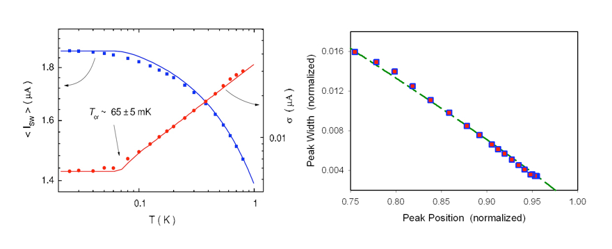
Figure 51: Left panel: Fig.2 from Yu showing experimental SCD peak posions (blue squares) and peak widths (red circles) as functions of temperature; Right panel: Dashed line - SCD peak positions versus peak widths from simulations described in II-C, and the experimental data shown in the left panel (blue/red squares).

Therefore the most appropriate consideration of experimental data would use peak positions and a linear temperature scale

References

- (1) B.D. Josephson, Possible New Effects in Superconductive Tunnelling, Physics Letters 1 (1962) 251-253.
- (2) M. Gurwitch, W.A. Washington, and H.A. Huggins, “High qualityrefractory Josephson tunnel junctions utilizing thin aluminum layers”,Appl. Phys. Lett. 42, (1983),472-474
- (3) L. Solymar, Superconductive Tunnelling and Applications, Chapman and Hall(1972)
- (4) M. Fiske, Temperature and magnetic field dependences of the Josephson tunneling current, Rev. Mod. Phys. 36 (1964) 221-222.
- (5) V. Ambegaokar and A. Baratoff, Tunneling Between Superconductors, Phys. Rev. Lett. 10, (1963) 486-489 [Erratum: Phys. Rev. Lett. 11, (1963) 104)].
- (6) P. W. Anderson, Special Effects in Superconductivity, in Lectures on the Many Body Problem, Vol. 2, edited by E. R. Caianiello,Academic Press (1964) pp 113-135
- (7) A.J. Leggett, Macroscopic Quantum Systems and the Theory of Quantum Measurement, Suppl. Prog. Theor. Phys.69 (1980) 80-100.
- (8) A. Barone and G. Paterno, Physics and Applications of the Josephson Effect, Wiley-Interscience (1982).
- (9) W.C. Stewart, Current-Voltage Characteristics of Josephson Junctions, Applied Physics Letters 12 (1968) 277-280.
- (10) D.E. McCumber, Effect of ac Impedance on dc Voltage-Current Characteristics of Superconductor Weak-Link Junctions, Journal of Applied Physics 39 (1968) 3113-3118.
- (11) T. Van Duzer and C.W. Turner, Principles of Superconductive Devices and Circuits, Elsevier (1981).
- (12) reproduced from R. Gross and A. Marx, Applied Superconductivity: Josephson Effect and Superconducting Electronics, Lecture Notes TU MUnich (2005).
- (13) N. Grønbech-Jensen, M.G. Castellano, F. Chiarello, M. Cirillo, C. Cosmelli, V. Merlo, R. Russo, and G. Torrioli, Anomalous thermal escape in Josephson systems perturbed by microwaves in B. Ruggiero, P. Delsing, C. Granata, Y. Pashkin, and P. Silvestrini (Eds.), Quantum Computing in Solid State Systems, Springer N.Y.(2006) ISBN 978-1-4419-2089-8, pp 111-119; arXiv.cond-mat/0412692v1 (eqs. 11, 13).
- (14) F.M.S. Lima and P. Arun, An accurate formula for the period of a simple pendulum oscillating beyond the small angle regime, arXiv.physics/0510206v3 (2006); G.L. Baker and J.A Blackburn, The Pendulum: a case study in physics, Oxford University Press (2005), page 47.
- (15) J.A. Blackburn, M. Cirillo, and N. Grønbech-Jensen, Classical statistical model for distributions of escape events in swept-bias Josephson junctions, Phys. Rev. B 85 (2012) 104501-1 to 104501-7
- (16) M. G. Castellano, G. Torrioli, C. Cosmelli, A. Costantini, F. Chiarello, P. Carelli, G. Rotoli, M. Cirillo, R. L. Kautz, Thermally Activated Escape from the Zero-Voltage State in Long Josephson Junctions, Phys. Rev. B54, (1996) 15417-15428
- (17) N. Grønbech-Jensen, D. B. Thompson, M. Cirillo, and C. Cosmelli, Thermal Escape from Zero-Voltage States in Hysteretic Superconducting Interferometers, Phys. Rev. B67,(2003) 2245051-2245056
- (18) S. Barbanera, M. G. Castellano, G. Torrioli, and M. Cirillo, A Probe for the Investigation of the Superconducting Metastable State in YBCO Step-Edge Junctions, Appl. Phys. Lett. 72, (1998) 1760-1762.
- (19) I. Affleck, Quantum-Statistical Metastability, Phys. Rev. Lett. 46, (1981) 388.
- (20) M.H. Devoret, J.M. Martinis, and J. Clarke, Measurements of Macroscopic Quantum Tunneling out of the Zero-Voltage State of a Current-Biased Josephson Junction, Phys. Rev. Lett. 55 (1985) 1908-1911; J.M. Martinis, M.H. Devoret, and J. Clarke, Experimental tests for the quantum behavior of a macroscopic degree of freedom: The phase difference across a Josephson junction, Phys. Rev. B 35 (1987) 4682-4698; J. Clarke, A.N. Cleland, M.H. Devoret, D. Esteve, and J.M. Martinis, Quantum Mechanics of a Macroscopic Variable: The Phase Difference of a Josephson Junction, Science 239 (1988) 992-997.
- (21) .H.F. Yu, X.B. Zhu, Z.H. Peng, W.H. Cao, D.J. Cui, Ye Tian, G.H. Chen, D.N. Zheng, X.N. Jing, Li Lu, S.P. Zhao, and S. Han, Quantum and classical resonant escapes of a strongle driven Josephson junction, Phys. Rev. B 81 (2010) 144518-1 to 144518-9
- (22) R.F. Voss and R.A. Webb, Macroscopic Quantum Tunneling in 1m Nb Josephson Junctions, Phys. Rev. Lett. 47 (1981) 265-268.
- (23) J.A. Blackburn, M. Cirillo, and N. Grønbech-Jensen, Switching current distributions in Josephson junctions at very low temperatures, European Physics Letters 107 (2014), 67001 (5 pages).
- (24) X.Y. Jin, A. Kamal, A.P. Sears, T. Gudmundsen, D. Hover, J. Miloshi, R. Slattery, F. Yan, J. Yoder, T.P. Orlando, S. Gustavsson, and W.D. Oliver, Thermal and Residual Excited-State Population in a 3D Transmon Qubit, Phys. Rev. Lett. 114 (2015) 240501 7 pages.
- (25) R. Cristiano and P. Silvestrini, Experiments on Macroscopic Quantum Tunnelling in Josephson Structures: Influence of the Uncertainty of Junction Parameters, Il Nuovo Cimento Note Brevi 10 (1988) 869-874.
- (26) P. Silvestrini, Comment on “Measurements of Macroscopic Quantum Tunneling out of the Zero-Voltage State of a Current-Biased Josephson Junction, Phys. Rev. Lett. 63, (1989) 211.
- (27) M.H. Devoret, J.M. Martinis, and J. Clarke, Reply in Phys. Rev. Lett. 63, (1989) 212.
- (28) P. Silvestrini, Comments about the Escape Temperature Representation of Experiments on Macroscopic Quantum Tunnelling, Il Nuovo Cimento Note Brevi 11 (1989) 897-901.
- (29) J.A. Blackburn, M. Cirillo, and N. Grønbech-Jensen, On the classical model for microwave induced escape from a Josephson washboard potential, Phys. Lett. A 374 (2010) 2827-2830.
- (30) A. Wallraff, T. Duty, A. Lukashenko, and A.V. Ustinov, Multiphoton Transitions between Energy Levels in a Current-Biased Josephson Tunnel Junction, Phys. Rev. Lett. 90 (2003) 037003 4 pages.
- (31) I.Q. You and F. Nori, Atomic physics and quantum optics using superconducting circuits, Nature 474 (2011) 589-597.
- (32) J.M. Martinis, M.H. Devoret, and J. Clarke, Energy-Level Quantization in the Zero-Voltage State of a Current-Biased Josephson Junction, Phys. Rev. Lett. 55 (1985) 1543-1546.
- (33) A.J. Berkley, H. Xu, M.A. Gubrud, R.C. Ramos, J.R. Anderson, C.J. Lobb, and F.C. Wellstood, Decoherence in a Josephson-junction qubit, Phys. Rev. B 68 (2003) 060502(R) 4 pages.
- (34) Z.E. Thrailkill, J.G. Lambert, S.A. Carabello, and R.C. Ramos, private communication (2012) from R.C. Ramos.
- (35) P. Silvestrini, V. G. Palmieri, B. Ruggiero, and M. Russo, Observation of Energy Levels Quantization in Underdamped Josephson Junctions above the Classical-Quantum Regime Crossover Temperature, Phys. Rev. Lett. 79 (1997) 3046-3049.
- (36) N. Grønbech-Jensen, M.G. Castellano, F. Chiarello, M. Cirillo, C. Cosmelli, L.V. Filippenko, R. Russo,and G. Torrioli, Microwave-Induced Thermal Escape in Josephson Junctions, Phys. Rev. Lett. 93 (2004) 1070021-1070024.
- (37) N. Grønbech-Jensen and M. Cirillo, ac-induced thermal vortex escape in magnetic-field-embedded long annular Josephson junctions, Phys. Rev. B 70 (2004) 214507, 7 pages.
- (38) A. Davidson, B. Dueholm, B. Kryger, and N. F. Pedersen,Experimental Investigation of Trapped Sine-Gordon Solitons, Phys. Rev. Lett. 55, (1985) 2059- 2062 (four pages).
- (39) A.V. Ustinov and N. Thyssen, Experimental Study of Fluxon Dynamics in a Potential Well, Journal of Low Temperature Physics 106 (1997) 193-200.
- (40) N. Martucciello, J. Mygind, V.P. Koshelets, A.V. Shchukin, L.V. Filippenko, and R. Monaco, Fluxon dynamics in long annular Josephson tunnel junctions, Phys. Rev. B 57 (1998) 5444-5449.
- (41) A. Wallraff, A. Lukashenko, J. Lisenfeld, A. Kemp, M.V. Fistul, Y. Koval, and A.V. Ustinov, Quantum dynamics of a single vortex, Nature 425 (2003), 155-158.
- (42) A. J. Leggett, Macroscopic Quantum Tunnelling and Related Matters, Jpn. J. Appl. Phys., 26, (1987)1986-1993.
- (43) W. Shor, Polynomial time algorithms for prime factorization and discrete logarithms on a quantum computer, SIAM J. on Computing, 26, (1997)1484 – 1509.
- (44) L. K. Grover, From Schrodinger’s equation to quantum search algorithm, American Journal of Physics, 69, (2001) 769-777.
- (45) J.M. Martinis, S. Nam, J. Aumentado, and C. Urbina, Rabi Oscillations in a Large Josephson-Junction Qubit, Phys. Rev. Lett. 89 (2002) 117901 4 pages
- (46) I. I. Rabi, Space Quantization in a Gyrating Magnetic Field, Phys. Rev. 51, (1937)652-654
- (47) R. Loudon, The Quantum Theory of Light, Oxford Science Publications (Oxford UK, 2000), see in particular sect. 2.7
- (48) N. Grønbech-Jensen and M. Cirillo, Rabi-Type Oscillations in a Classical Josephson Junction, Phys. Rev. Lett. 95 (2005) 067001 4 pages.
- (49) J.E. Marchese, M. Cirillo, and N.Grønbech Jensen, Classical analysis of phase-locking transients and Rabi-type oscillations in microwave-driven Josephson junctions, Phys. Rev. B 73 (2006) 174507 8 pages
- (50) J. Claudon, F. Balestro, F.W. J. Hekking, and O. Buisson, Coherent Oscillations in a Superconducting Multilevel Quantum SystemPhys. Rev. Lett. 93, (2004) 1870031-18700314 (four pages).
- (51) D. Vion, A. Aasime, A. Cottet, P. Joyez, H. Pothier, C. Urbina, D. Esteve, M.H. Devoret,Rabi oscillations, Ramsey fringes and spin echoes in an electrical circuit ,Fortschr. Phys. 51, (2003) 462-468 (seven pages)
- (52) B. L. T. Plourde, T. L. Robertson, P. A. Reichardt, T. Hime, S. Linzen, C.-E. Wu, and John Clarke, Flux qubits and readout device with two independent flux lines, Phys. Rev. B 72 (2005) 0605061-06050614
- (53) N. F. Ramsey, A Molecular Beam Resonance Method with Separated Oscillating Fields,Phys. Rev. 78, (1950) 695-699.
- (54) L. Hahn, Spin echoes, Physical Review 80, (1950) 580–594
- (55) J. E. Marchese, M. Cirillo, and N. Grønbech-Jensen, Simulating Ramsey-Type Fringes in a Pulsed Microwave-Driven Classical Josephson Junction, Open Systems and Information Dynamics 14 (2007) 189-196.
- (56) J. E. Marchese, M. Cirillo, and N. Grønbech-Jensen,Classical analogs for Rabi-oscillations, Ramsey-fringes, and spin-echo in Josephson junctions, European Physical Journal Special Topics 147 (2007) 333-342.
- (57) J. E. Marchese, M. Cirillo, and N. Grønbech-Jensen, Investigation of resonant and transient phenomena in Josephson junction flux qubits, Phys. Rev. B79 (2009) 0945171-0945178.
- (58) M.Steffen, M. Ansmann, R.C. Bialczak, N. Katz, E. Lucero, R. McDermott, M. Neeley, E.M. Weig, A.N. Cleland, and J.M. Martinis, Measurement of the Entanglement of Two Superconducting Qubits via State Tomography, Science 313 (2006) 1423-1425.
- (59) J.A. Blackburn, J.E. Marchese, M. Cirillo, and N. Grønbech-Jensen, Classical analysis of capacitively coupled superconducting qubits, Phys. Rev. B 79 (2009) 054516, 5 pages.
- (60) T. L. Chow, Classical Mechanics, Wiley, New York, 1995, Fig.11.4, page 395.
- (61) N. Grønbech-Jensen, J.E. Marchese, M. Cirillo, and J.A. Blackburn, Tomography and Entanglement in Coupled Josephson Junction Qubits, Phys. Rev. Lett. 105 (2010),010501- 4 pages.
- (62) R. Hallock, Is solid helium a supersolid?, Physics Today 68 (5), (2015) 30-35.
- (63) R. L. Kautz and R. Monaco, Survery of Chaos in the rf-Biased Josephson Junction, J.Appl. Phys. 57, (1985) 875-889 (15 pages).
- (64) “Structure, Coherence and Chaos in Dynamical Systems”, Edited by P. L. Christiansen and R. D. Parmentier, Manchester Univ. Press. 1989.
- (65) P. Carelli, M. G. Castellano, F. Chiarello, L. Chiatti, M. Cirillo, C. Cosmelli,G. Diambrini Palazzi, D. Fargion, R. Leoni, G. Rotoli, F. Scaramuzzi and G. Torrioli, MQC : An Experiment for Detecting Macroscopic Quantum Coherence with a System of SQUIDs, Annals of the New York Academy of Sciences 775 (1995) 845-847.
- (66) C. D. Tesche, Can a Noninvasive Measurement of Magnetic Flux be Performed with Superconducting Circuits?, Phys. Rev. Lett. 64 (1990) 2358-2361.
- (67) S. Han, J. Lapointe, and J. E. Lukens, Effect of a Two-Dimensional Potential on the Rate of Thermally Induced Escape Over the Potential Barrier, Phys. Rev. B46 (1992) 6338-6345.
- (68) J. R. Friedman, V. Patel, W. Chen, S. K. Tolpygo, and J. E. Lukens, Quantum Superposition of Distinct Macroscopic States, Nature 406 (2000) 43-45.
- (69) M. G. Castellano, F. Chiarello, R. Leoni, F. Mattioli, G. Torrioli, P. Carelli, M. Cirillo, C. Cosmelli, A. de Waard, G. Frossati, N. Grønbech-Jensen, and S. Poletto, Catastrophe Observation in a Josephson-Junction System, Phys. Rev. Lett. 98, (2007) 170021-170024 (four pages)
- (70) R. Thom, “Structural Stability and Morphogenesis” (Benjamin, Reading, MA, 1975).
- (71) F. Chiarello, S. Spilla, M. G. Castellano, C. Cosmelli, A. Messina, R. Migliore, A. Napoli, and G. Torrioli, Resonant effects in a SQUID qubit subjected to nonadiabatic changes,Phys. Rev. B 89, (2014) 134506 (six pages)
- (72) N. Roch, M.E. Schwartz, F. Motzoi, C. Macklin, R. Vijay, A.W. Eddins, A.N. Korotkov, K.B. Whaley, M. Saraovar, and I. Siddiqi, Observation of Measurement-induced Entanglement and Quantum Trajectories of Remote Superconducting Qubits, Phys. Rev. Lett. 112 (2014) 170501- 5 pages.
- (73) J. Koch, T.M. Yu, J. Gambetta, A.A. Houck, D.J. Schuster, J. Majer, A. Blais, M.H. Devoret, S.M. Girvin, and R.J. Schoelkopf, Charge-insensitive qubit design derived from the Cooper pair box, Phys. Rev. A 76, (2007) 042319-19 pages.
- (74) Philip Krantz, Investigation of Transmon Qubit Designs - A Study of Plasma Frequency Predictability, M Sc Thesis, Chalmers University of Technology, Gothenburg, Sweden.