Choice by Elimination via Deep Neural Networks

Abstract

We introduce Neural Choice by Elimination, a new framework that integrates deep neural networks into probabilistic sequential choice models for learning to rank. Given a set of items to chose from, the elimination strategy starts with the whole item set and iteratively eliminates the least worthy item in the remaining subset. We prove that the choice by elimination is equivalent to marginalizing out the random Gompertz latent utilities. Coupled with the choice model is the recently introduced Neural Highway Networks for approximating arbitrarily complex rank functions. We evaluate the proposed framework on a large-scale public dataset with over $425K$ items, drawn from the Yahoo! learning to rank challenge. It is demonstrated that the proposed method is competitive against state-of-the-art learning to rank methods.

1 Introduction

People often rank options when making choice. Ranking is central in many social and individual contexts, ranging from election [16], sports [17], information retrieval [22], question answering [1], to recommender systems [32]. We focus on a setting known as learning to rank (L2R) in which the system learns to choose and rank items (e.g. a set of documents, potential answers, or shopping items) in response to a query (e.g., keywords, a question, or an user).

Two main elements of a L2R system are rank model and rank function. One of the most promising rank models is listwise [22] where all items responding to the query are considered simultaneously. Most existing work in L2R focuses on designing listwise rank losses rather than formal models of choice, a crucial aspect of building preference-aware applications. One of a few exceptions is the Plackett-Luce model which originates from Luce’s axioms of choice [24] and is later used in the context of L2R under the name ListMLE [34]. The Plackett-Luce model offers a natural interpretation of making sequential choices. First, the probability of choosing an item is proportional to its worth. Second, once the most probable item is chosen, the next item will be picked from the remaining items in the same fashion.

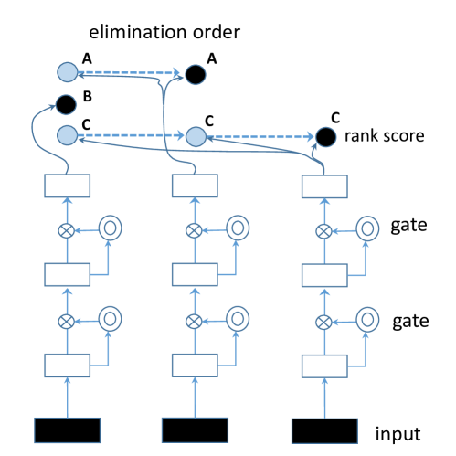
Figure 1: Neural choice by elimination with 4-layer highway networks for ranking three items (A,B,C). Empty boxes represent hidden layers that share the same parameters (hence, recurrent). Double circles are gate that controls information flow. Dark filled circles represent a chosen item at each step – here the elimination order is (B,A,C).

However, the Plackett-Luce model suffers from two drawbacks. First, the model spends effort to separate items down the rank list, while only the first few items are usually important in practice. Thus the effort in making the right ordering should be spent on more important items. Second, the Plackett-Luce is inadequate in explaining many competitive situations, e.g., sport tournaments and buying preferences, where the ranking process is reversed – worst items are eliminated first [33].

Addressing these drawbacks, we introduce a probabilistic sequential rank model termed choice by elimination. At each step, we remove one item and repeat until no item is left. The rank of items is then the reverse of the elimination order. This elimination process has an important property: Near the end of the process, only best items compete against the others. This is unlike the selection process in Plackett-Luce, where the best items are contrasted against all other alternatives. We may face difficulty in separating items of similarly high quality but can ignore irrelevant items effortlessly. The elimination model thus reflects more effort in ranking worthy items.

Once the ranking model has been specified, the next step in L2R is to design a rank function $f(\mathit{\bm{x}})$ of query-specific item attributes $\mathit{\bm{x}}$ [22]. We leverage the newly introduced highway networks [28] as a rank function approximator. Highway networks are a compact deep neural network architecture that enables passing information and gradient through hundreds of hidden layers between input features and the function output. The highway networks coupled with the proposed elimination model constitute a new framework termed Neural Choice by Elimination (NCE) illustrated in Fig. 1.

The framework is an alternative to the current state-of-the-arts in L2R which involve tree ensembles [12, 5, 4] trained with hand-crafted metric-aware losses [7, 21]. Unlike the tree ensembles where typically hundreds of trees are maintained, highway networks can be trained with dropouts [27] to produce an implicit ensemble with only one thin network. Hence we aim to establish that deep neural networks are competitive in L2R. While shallow neural networks have been used in ranking before [6], they were outperformed by tree ensembles [21]. Deep neural nets are compact and more powerful [3], but they have not been measured against tree-based ensembles for generic L2R problems. We empirically demonstrate the effectiveness of the proposed ideas on a large-scale public dataset from Yahoo! L2R challenge with totally $18.4$ thousands queries and $425$ thousands documents.

To summarize, our paper makes the following contributions: (i) introducing a new neural sequential choice model for learning to rank; and (ii) establishing that deep nets are scalable and competitive as rank function approximator in large-scale settings.

2 Background

2.1 Related Work

The elimination process has been found in multiple competitive situations such as multiple round contests and buying decisions [14]. Choice by elimination of distractors has been long studied in the psychological literature, since the pioneer work of Tversky [33]. These backward elimination models may offer better explanation than the forward selection when eliminating aspects are available [33]. However, existing studies are mostly on selecting a single best choice. Multiple sequential eliminations are much less studied [2]. Second, most prior work has been evaluated on a handful of items with several attributes, whereas we consider hundreds of thousands of items with thousands of attributes. Third, the cross-field connection with data mining has not been made. The link between choice models and Random Utility Theory has been well-studied since Thurstone in the 1920s, and is still an active topic [2, 30, 31]. Deep neural networks for L2R have been studied in the last two years [18, 10, 26, 11, 25]. Our work contributes a formal reasoning of human choices together with a newly introduced highway networks which are validated on large-scale public datasets against state-of-the-art methods.

2.2 Plackett-Luce

We now review Plackett-Luce model [24], a forward selection method in learning to rank, also known in the L2R literature as ListMLE [34]. Given a query and a set of response items $\mathcal{I}=\left(1,2,..,N\right)$, the rank choice is an ordering of items $\mathit{\bm{\pi}}=(\pi_{1},\pi_{2},...,\pi_{N})$, where $\pi_{i}$ is the index of item at rank $i$. For simplicity, assume that each item $\pi_{i}$ is associated with a set of attributes, denoted as $\mathit{\bm{x}}_{\pi_{i}}\in\mathbb{R}^{p}$. A rank function $f(\mathit{\bm{x}}_{\pi_{i}})$ is defined on $\pi_{i}$ and is independent of other items. We aim to characterize the rank permutation model $P(\mathit{\bm{\pi}})$.

Let us start from the classic probabilistic theory that any joint distribution of $N$ variables can be factorized according to the chain-rule as follows

$$P(\mathit{\bm{\pi}})=P(\pi_{1})\prod_{i=2}^{N}P(\pi_{i}\mid\bm{\pi}_{1:i-1})$$ (1)

where $\bm{\pi}_{1:i-1}$ is a shorthand for $(\pi_{1},\pi_{2},..,\pi_{i-1})$, and $P(\pi_{i}\mid\bm{\pi}_{1:i-1})$ is the probability that item $\pi_{i}$ has rank $i$ given all existing higher ranks $1,...,i-1$. The factorization can be interpreted as follows: choose the first item in the list with probability of $P(\pi_{1})$, and choose the second item from the remaining items with probability of $P(\pi_{2}|\pi_{1})$, and so on. Luce’s axioms of choice assert that an item is chosen with probability proportional to its worth. This translates to the following choice model:

$$P(\pi_{i}\mid\bm{\pi}_{1:i-1})=\frac{\exp\left(f(\mathit{\bm{x}}_{\pi_{i}})\right)}{\sum_{j=i}^{N}\exp\left(f(\mathit{\bm{x}}_{\pi_{j}})\right)}$$

Learning using maximizing likelihood minimizes the log-loss:

$$\ell_{1}(\mathit{\bm{\pi}}) =\sum_{i=1}^{N-1}\left(-f(\mathit{\bm{x}}_{\pi_{i}})+\log\sum_{j=i}^{N}\exp\left(f(\mathit{\bm{x}}_{\pi_{j}})\right)\right)$$ (2)

3 Choice by Elimination

We note that the factorization in Eq. (1) is not unique. If we permute the indices of items, the factorization still holds. Here we derive a reverse Plackett-Luce model as follows

$$P(\mathit{\bm{\pi}})=Q(\pi_{N})\prod_{i=1}^{N-1}Q(\pi_{i}\mid\bm{\pi}_{i+1:N})$$ (3)

where $Q(\pi_{i}\mid\bm{\pi}_{i+1:N})$ is the probability that item $\pi_{i}$ receives rank $i$ given all existing lower ranks $i+1,i+2,...,N$

Since $\pi_{N}$ is the most irrelevant item in the list, $Q(\pi_{N})$ can be considered as the probability of eliminating the item. Thus the entire process is backward elimination: The next irrelevant item $\pi_{k}$ is eliminated, given that more extraneous items ($\mathit{\bm{\pi}}_{i>k)}$) have already been eliminated. It is reasonable to assume that the probability of an item being eliminated is inversely proportional to its worth. This suggests the following specification

$$Q(\pi_{i}|\bm{\pi}_{i+1:N}) = \frac{\exp\left(-f(\mathit{\bm{x}}_{\pi_{i}})\right)}{\sum_{j=1}^{i}\exp\left(-f(\mathit{\bm{x}}_{\pi_{j}})\right)}.$$ (4)

Note that, due to specific choices of conditional distributions, distributions in Eqs. (1,3) are generally not the same. With this model, the log-loss has the following form:

$$\ell_{2}(\mathit{\bm{\pi}}) =\sum_{i=1}^{N}\left(f(\mathit{\bm{x}}_{\pi_{i}})+\log\sum_{j=1}^{i}\exp\left(-f(\mathit{\bm{x}}_{\pi_{j}})\right)\right)$$ (5)

3.1 Derivation using Random Utility Theory.

Random Utility Theory [2, 29] offers an alternative that explains the ordering of items. Assume that there exists latent utilities $\left\{u_{i}\right\}$, one per item $\left\{\pi_{i}\right\}$. The ordering $P^{*}(\mathit{\bm{\pi}})$ is defined as $\Pr\left(u_{1}\geq u_{2}\geq...\geq u_{N}\right)$. Here we show that it is linked to Gompertz distribution. Let $u_{j}\geq 0$ denote the latent random utility of item $\pi_{j}$. Let $v_{j}=e^{bu_{j}}$, the Gompertz distribution has the PDF $P_{j}(u_{j})=b\eta_{j}v_{j}\exp\left(-\eta_{j}v_{j}+\eta_{j}\right)$ and the CDF $F_{j}(u_{j})=1-\exp\left(-\eta_{j}(v_{j}-1)\right)$, where $b>0$ is the scale and $\eta>0$ is the shape parameter.

At rank $i$, choosing the worst item $\pi_{i}$ translates to ensuring $u_{i}\leq u_{j}$ for all $j<i$. The random utility theory states that probability of choosing $\pi_{i}$ can be obtained by integrating out all latent utilities subject to the inequality constraints:

$$Q(\pi_{i}\mid\bm{\pi}_{i+1:N}) = \int_{0}^{+\infty}P_{i}(u_{i})\left[\int_{u_{i}}^{+\infty}\prod_{j<i}P_{j}(u_{j})du_{j}\right]du_{i}$$

$$= \int_{0}^{+\infty}P_{i}(u_{i})\prod_{j<i}\left(1-F_{j}(u_{i})\right)du_{i}$$

$$= \int_{0}^{+\infty}b_{i}\eta_{ii}v_{i}\exp\left(-v_{i}\sum_{j\leq i}\eta_{ij}+\sum_{j\leq i}\eta_{ij}\right)du_{i}$$

Note that we have used $\eta_{ij}$ instead of $\eta_{j}$ since this location parameter is specific to rank $i$. Defining $\eta_{ij}=\exp\left(-f(\mathit{\bm{x}}_{\pi_{j}})\right)$ and changing the variable from $u_{i}$ to $v_{i}$ gives us:

$$Q(\pi_{i}\mid\bm{\pi}_{i+1:N}) =\int_{1}^{+\infty}\eta_{ii}\exp\left(-v_{i}\sum_{j\leq i}\eta_{ij}+\sum_{j\leq i}\eta_{ij}\right)dv_{i}$$

$$=\frac{\eta_{ii}e^{\sum_{j\leq i}\eta_{j}}}{\sum_{j\leq i}\eta_{ij}}\int_{1}^{+\infty}\exp\left(-v_{i}\sum_{j\leq i}\eta_{ij}\right)dv_{i}$$

$$=\frac{\eta_{ii}}{\sum_{j\leq i}\eta_{ij}}=\frac{\exp\left(-f(\mathit{\bm{x}}_{\pi_{i}})\right)}{\sum_{j=1}^{i}\exp\left(-f(\mathit{\bm{x}}_{\pi_{j}})\right)}.$$

This resembles Eq. (4).

Remark:

We note in passing that in case of plain Plackett-Luce, $P(\mathit{\bm{\pi}})\equiv P^{*}(\mathit{\bm{\pi}})$ if and only if $u_{\pi_{j}}$ is drawn from a Gumbel distribution of location $f(\mathit{\bm{x}}_{\pi_{j}})$ and scale $1$ for all $j=1,2,...,N$ [23, 35].

3.2 Linear time learning

We show that both the loss and its functional gradient can be computed in linear time. Let $\phi_{i}=\exp\left(-f(\mathit{\bm{x}}_{\pi_{i}})\right)$, $Z_{i}=\sum_{j=1}^{i}\phi_{j}=\phi_{i}+Z_{i-1}$ , and $Y_{i}=\sum_{j=1}^{i}1/Z_{j}$. The loss in Eq. (5) becomes $\ell_{2}(\mathit{\bm{\pi}})=\sum_{i=1}^{N}\left(f(\mathit{\bm{x}}_{\pi_{i}})+\log Z_{i}\right)$ which can be evaluated in linear time. The functional gradient is reduced to $\partial_{f_{k}}\ell_{2}=\gamma_{k}\left(1-\phi_{k}Y_{k}\right)$, which is constant for each $k$.

4 Neural Highway Networks for Rank Function

Once the rank models have been specified, it remains to define the rank function $f(\mathit{\bm{x}})$. We propose the novel use of neural highway networks [28] to approximate $f(\mathit{\bm{x}})$, under the new ranking loss functions proposed in Eqs. (2,5). Highway networks are powerful, compact function approximator that overcomes the major bottleneck of standard deep neural networks: with increasing depth, it is much harder to pass information and gradient between input and output. More specifically, highway networks are a special neural network of $L$ nonlinear projection layers, of which $L-1$ layers are recurrent. At the bottom, the data is projected into a $K$-dimensional space $\mathit{\bm{z}}=g\left(\mathit{\bm{b}}_{H}+W_{X}\mathit{\bm{x}}\right)$, where $g$ is an element-wise non-linear transform. Subsequent layers are recursive same-dimensional projections:

$$\mathit{\bm{z}}_{l+1} \leftarrow H(\mathit{\bm{z}}_{l})\ast T(\mathit{\bm{z}}_{l})+\mathit{\bm{z}}_{l}\ast\left(1-T(\mathit{\bm{z}}_{l})\right)$$

where $H(\mathit{\bm{z}})=g\left(\mathit{\bm{b}}_{H}+W_{H}\mathit{\bm{z}}\right)$, $T(\mathit{\bm{z}})\in\left[0,1\right]^{K}$ is an element-wise gating function, and $\ast$ denotes element-wise product. The gate $T(\mathit{\bm{z}})$ allows information to pass freely when $T(\mathit{\bm{z}})=0$ and forces total nonlinear transforms when $T(\mathit{\bm{z}})=1$. A typical implementation is $T(\mathit{\bm{z}})=\sigma\left(\mathit{\bm{b}}_{T}+W_{T}\mathit{\bm{z}}\right)$, where $\sigma$ is the sigmoid function. At the top layer, we have $f(\mathit{\bm{x}})=\left\langle\mathit{\bm{w}},\mathit{\bm{z}}_{L}\right\rangle$. Note that when the number of hidden layer is 1, this returns to the standard shallow neural network; and when $T(\mathit{\bm{z}})=1$, the highway network becomes a recurrent network. Let $\bm{\theta}=\left(\mathit{\bm{b}}_{T},\mathit{\bm{b}}_{H},W_{T},W_{H},W_{X},\mathit{\bm{w}}\right)$ be model parameters, gradient-based learning proceeds as follows:

$$\bm{\theta}\leftarrow\bm{\theta}-\frac{\mu}{N}\sum_{k=1}^{N}\frac{\partial\ell_{1,2}}{\partial f(\mathit{\bm{x}}_{\pi_{k}})}\frac{\partial f(\mathit{\bm{x}}_{\pi_{k}})}{\partial\bm{\theta}}$$

for learning rate $\mu>0$, where $\frac{\partial\ell_{1,2}}{\partial f(\mathit{\bm{x}}_{\pi_{k}})}$ are functional gradients derived from Eqs. (2,5).

5 Experimental Evaluation

5.1 Data & Evaluation Metrics

We validate the proposed model using a large-scale Web dataset from the Yahoo! learning to rank challenge [8], . The dataset is split into a training set of $18,425$ queries ($425,821$ documents), and a testing set of $1,520$ queries ($47,313$ documents). We also prepare a smaller training subset, called Yahoo!-small, which has $1,568$ queries and $47,314$ documents. The Yahoo! datasets contain the groundtruth relevance scores (from $0$ for irrelevant to $4$ for perfectly relevant). There are $519$ pre-computed unique features for each query-document pair. We normalize the features across the whole training set to have mean $0$ and standard deviation $1$.

Two evaluation metrics are employed. The Normalized Discount Cumulative Gain [19] is defined as:

$$NG@T=\frac{1}{N_{max}}\sum_{i=1}^{T}\frac{2^{r_{\pi_{i}}}-1}{\log_{2}(1+i)}$$

where $r_{\pi_{i}}$ is the relevance of item at rank $i$. The other metric is Expected Reciprocal Rank (ERR) [9], which was used in the Yahoo! learning-to-rank challenge (2011):

$$ERR =\sum_{i}\frac{R(r_{\pi_{i}})}{i}\prod_{j>i}\left[1-R(r_{\pi_{j}})\right],\,\mbox{s.t.}\,R(r_{\pi_{i}})=\frac{2^{r_{\pi_{i}}}-1}{16}$$

Both metrics discount for the long list and place more emphasis on the top ranking. Finally, all metrics are averaged across all test queries.

5.2 Model Implementation

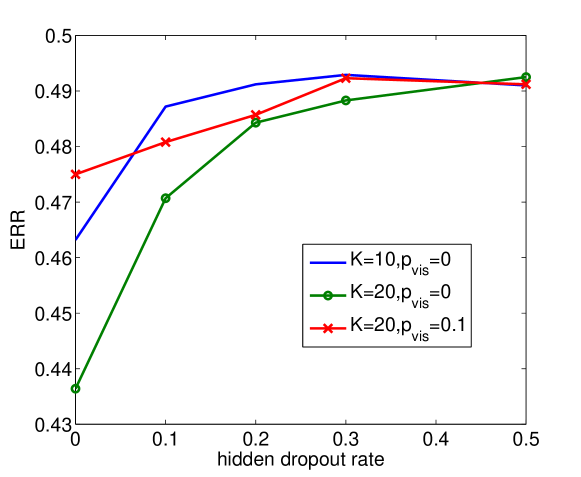
Figure 2: Effect of dropouts on NCE performance of a $3$-layer highway nets on Yahoo! small set. $K$ is number of hidden units, $p_{vis}$ is dropout rate for visible layer.

The highway nets are configured as follows. Unless stated otherwise, we use ReLU units for transformation $H(\mathit{\bm{z}})$. Parameters $W_{1},W_{H}$ and $W_{T}$ are initialized randomly from a small Gaussian. Gate bias $\mathit{\bm{b}}_{T}$ is initialized at $-1$ to encourage passing more information, as suggested in [28]. Transform bias $\mathit{\bm{b}}_{H}$ is initialized at $0$. To prevent overfitting, dropout [27] is used, i.e., during training for each item in a mini-batch, input features and hidden units are randomly dropped with probabilities $p_{vis}$ and $p_{hid}$, respectively. As dropouts may cause big jumps in gradient and parameters, we set max-norm per hidden unit to $1$. The mini-batch size is 2 queries, the learning rate starts from $0.1$, and is halved when there is no sign of improvement in training loss. Learning stops when learning rate falls below $10^{-4}$. We fix the dropout rates as follows: (a) for small Yahoo! data, $p_{vis}=0$, $p_{hid}=0.3$ and $K=10$; (b) for large Yahoo! data, $p_{vis}=0$, $p_{hid}=0.2$ and $K=20$. Fig. 2 shows the effect of dropouts on the NCE model on the small Yahoo! dataset.

5.3 Results

5.3.1 Performance of choice models.

	Yahoo!-small			Yahoo!-large
Rank model	ERR	NDCG@1	NDCG@5	ERR	NDCG@1	NDCG@5
Rank SVM	0.477	0.657	0.642	0.488	0.681	0.666
Plackett-Luce	0.489	0.683	0.652	0.495	0.699	0.671
Choice by elimination	0.497	0.697	0.664	0.503	0.709	0.680

Table 1: Performance with linear rank functions.

In this experiment we ask whether the new choice by elimination model has any advantage over existing state-of-the-arts (the forward selection method of Plackett-Luce [34] and the popular Rank SVM [20]). Table 1 reports results on the all datasets (Yahoo!-small, Yahoo!-large) on different sequential models. The NCE works better than Rank SVM and Plackett-Luce. Note that due to the large size, the differences are statistically significant. In fact, in the Yahoo! L2R challenge, the top 20 scores (out of more than 1,500 teams) differ only by 1.56% in ERR, which is less than the difference between Plackett-Luce and choice by elimination (1.62%).

5.3.2 Neural nets versus gradient boosting.

	Placket-Luce			Choice by elimination
Rank function	ERR	NDCG@1	NDCG@5	ERR	NDCG@1	NDCG@5
SGTB	0.497	0.697	0.673	0.506	0.705	0.681
Neural nets	0.501	0.705	0.688	0.509	0.719	0.697

Figure 3: Comparing highway neural networks against stochastic gradient tree boosting (SGTB) on Yahoo!-large dataset.

We also compare the highway networks against the best performing method in the Yahoo! L2R challenge. Since it was consistently demonstrated that gradient boosting trees work best [8], we implement a sophisticated variant of Stochastic Gradient Tree Boosting (SGTB) [13] for comparison. In SGTB, at each iteration, regression trees are grown to fit a random subset of functional gradients $\frac{\partial\ell}{\partial f(\mathit{\bm{x}})}$. Grown trees are added to the ensemble with an adaptive learning rate which is halved whenever the loss fluctuates and does not decrease. At each tree node, a random subset of features is used to split the node, following [4]. Tree nodes are split at random as it leads to much faster tree growing without hurting performance [15]. The SGTB is configured as follows: number of trees is $300$; learning rate starts at $0.1$; a random subset of $50\%$ data is used to grow a tree; one third of features are randomly selected at each node; trees are grown until either the number of leaves reaches $512$ or the node size is below $40$.

Table. 3 show performance scores of models trained under different losses on the Yahoo!-large dataset. The highway neural networks are consistently competitive against the gradient tree boosting, the best performing rank function approximator in this challenge [8].

6 Conclusion

We have presented Neural Choice by Elimination, a new framework that integrates deep neural networks into a formal modeling of human behaviors in making sequential choices. Contrary to the standard Plackett-Luce model, where the most worthy items are iteratively selected, here the least worthy items are iteratively eliminated. Theoretically we show that choice by elimination is equivalent to sequentially marginalizing out Thurstonian random utilities that follow Gompertz distributions. Experimentally we establish that deep neural networks are competitive in the learning to rank domain, as demonstrated on a large-scale public dataset from the Yahoo! learning to rank challenge.

References

- [1] Arvind Agarwal, Hema Raghavan, Karthik Subbian, Prem Melville, Richard D Lawrence, David C Gondek, and James Fan. Learning to rank for robust question answering. In Proceedings of the 21st ACM international conference on Information and knowledge management, pages 833–842. ACM, 2012.
- [2] Hossein Azari, David Parks, and Lirong Xia. Random utility theory for social choice. In Advances in Neural Information Processing Systems, pages 126–134, 2012.
- [3] Yoshua Bengio. Learning deep architectures for AI. Foundations and trends® in Machine Learning, 2(1):1–127, 2009.
- [4] L. Breiman. Random forests. Machine learning, 45(1):5–32, 2001.
- [5] Leo Breiman. Bagging predictors. Machine Learning, 24(2):123–140, 1996.
- [6] C. Burges, T. Shaked, E. Renshaw, A. Lazier, M. Deeds, N. Hamilton, and G. Hullender. Learning to rank using gradient descent. In Proceedings of the 22nd international conference on Machine learning, page 96. ACM, 2005.
- [7] Christopher JC Burges, Krysta Marie Svore, Paul N Bennett, Andrzej Pastusiak, and Qiang Wu. Learning to rank using an ensemble of lambda-gradient models. In Yahoo! Learning to Rank Challenge, pages 25–35, 2011.
- [8] O. Chapelle and Y. Chang. Yahoo! learning to rank challenge overview. In JMLR Workshop and Conference Proceedings, volume 14, pages 1–24, 2011.
- [9] O. Chapelle, D. Metlzer, Y. Zhang, and P. Grinspan. Expected reciprocal rank for graded relevance. In CIKM, pages 621–630. ACM, 2009.
- [10] Li Deng, Xiaodong He, and Jianfeng Gao. Deep stacking networks for information retrieval. In Acoustics, Speech and Signal Processing (ICASSP), 2013 IEEE International Conference on, pages 3153–3157. IEEE, 2013.
- [11] Yuan Dong, Chong Huang, and Wei Liu. Rankcnn: When learning to rank encounters the pseudo preference feedback. Computer Standards & Interfaces, 36(3):554–562, 2014.
- [12] Jerome H. Friedman. Greedy function approximation: a gradient boosting machine. Annals of Statistics, 29(5):1189–1232, 2001.
- [13] J.H. Friedman. Stochastic gradient boosting. Computational Statistics and Data Analysis, 38(4):367–378, 2002.
- [14] Qiang Fu, Jingfeng Lu, and Zhewei Wang. ’reverse’ nested lottery contests. Journal of Mathematical Economics, 50:128–140, 2014.
- [15] Pierre Geurts, Damien Ernst, and Louis Wehenkel. Extremely randomized trees. Machine learning, 63(1):3–42, 2006.
- [16] Isobel Claire Gormley and Thomas Brendan Murphy. A mixture of experts model for rank data with applications in election studies. The Annals of Applied Statistics, 2(4):1452–1477, 2008.
- [17] RJ Henery. Permutation probabilities as models for horse races. Journal of the Royal Statistical Society, Series B, 43(1):86–91, 1981.
- [18] Po-Sen Huang, Xiaodong He, Jianfeng Gao, Li Deng, Alex Acero, and Larry Heck. Learning deep structured semantic models for web search using clickthrough data. In Proceedings of the 22nd ACM international conference on Conference on information & knowledge management, pages 2333–2338. ACM, 2013.
- [19] K. Järvelin and J. Kekäläinen. Cumulated gain-based evaluation of IR techniques. ACM Transactions on Information Systems (TOIS), 20(4):446, 2002.
- [20] T. Joachims. Optimizing search engines using clickthrough data. In Proceedings of the eighth ACM SIGKDD international conference on Knowledge discovery and data mining, pages 133–142. ACM New York, NY, USA, 2002.
- [21] P. Li, C. Burges, Q. Wu, JC Platt, D. Koller, Y. Singer, and S. Roweis. Mcrank: Learning to rank using multiple classification and gradient boosting. Advances in neural information processing systems, 2007.
- [22] Tie-Yan Liu. Learning to rank for information retrieval. springer, 2011.
- [23] D. McFadden. Conditional logit analysis of qualitative choice behavior. Frontiers in Econometrics, pages 105–142, 1973.
- [24] R.L. Plackett. The analysis of permutations. Applied Statistics, pages 193–202, 1975.
- [25] Aliaksei Severyn and Alessandro Moschitti. Learning to rank short text pairs with convolutional deep neural networks. In Proceedings of the 38th International ACM SIGIR Conference on Research and Development in Information Retrieval, pages 373–382. ACM, 2015.
- [26] Yang Song, Hongning Wang, and Xiaodong He. Adapting deep ranknet for personalized search. In Proceedings of the 7th ACM international conference on Web search and data mining, pages 83–92. ACM, 2014.
- [27] Nitish Srivastava, Geoffrey Hinton, Alex Krizhevsky, Ilya Sutskever, and Ruslan Salakhutdinov. Dropout: A simple way to prevent neural networks from overfitting. Journal of Machine Learning Research, 15:1929–1958, 2014.
- [28] Rupesh Kumar Srivastava, Klaus Greff, and Jürgen Schmidhuber. Training very deep networks. arXiv preprint arXiv:1507.06228, 2015.
- [29] L.L. Thurstone. A law of comparative judgment. Psychological review, 34(4):273, 1927.
- [30] T. Tran, D. Phung, and S. Venkatesh. Thurstonian Boltzmann Machines: Learning from Multiple Inequalities. In International Conference on Machine Learning (ICML), Atlanta, USA, June 16-21 2013.
- [31] T. Tran, D.Q. Phung, and S. Venkatesh. Sequential decision approach to ordinal preferences in recommender systems. In Proc. of the 26th AAAI Conference, Toronto, Ontario, Canada, 2012.
- [32] T. Truyen, D.Q Phung, and S. Venkatesh. Probabilistic models over ordered partitions with applications in document ranking and collaborative filtering. In Proc. of SIAM Conference on Data Mining (SDM), Mesa, Arizona, USA, 2011. SIAM.
- [33] Amos Tversky. Elimination by aspects: A theory of choice. Psychological review, 79(4):281, 1972.
- [34] F. Xia, T.Y. Liu, J. Wang, W. Zhang, and H. Li. Listwise approach to learning to rank: theory and algorithm. In Proceedings of the 25th international conference on Machine learning, pages 1192–1199. ACM, 2008.
- [35] John I Yellott. The relationship between Luce’s choice axiom, Thurstone’s theory of comparative judgment, and the double exponential distribution. Journal of Mathematical Psychology, 15(2):109–144, 1977.