Generalized Jensen Inequalities with Application to Stability Analysis of Systems with Distributed Delays over Infinite Time-Horizons

Abstract

The Jensen inequality has been recognized as a powerful tool to deal with the stability of time-delay systems. Recently, a new inequality that encompasses the Jensen inequality was proposed for the stability analysis of systems with finite delays. In this paper, we first present a generalized integral inequality and its double integral extension. It is shown how these inequalities can be applied to improve the stability result for linear continuous-time systems with gamma-distributed delays. Then, for the discrete-time counterpart we provide an extended Jensen summation inequality with infinite sequences, which leads to less conservative stability conditions for linear discrete-time systems with poisson-distributed delays. The improvements obtained thanks to the introduced generalized inequalities are demonstrated by examples.

1 Introduction

Time-delay often appears in many control systems either in the state, the control input, or the measurements. During the last two decades, the stability of time-delay systems has received considerable attention (e.g., [3], [8], [15], [17] and references therein). One of the most popular approaches is the use of Lyapunov-Krasovskii functionals (LKF) to derive stability conditions (e.g., [1], [5], [9], [26]). The choice of the Lyapunov functional and the method of bounding an integral term in the derivative of the LKF are important ways to reduce conservativeness of the stability results. The Jensen inequality [8], has been widely used as an efficient bounding technique, although at a price of an unavoidable conservativeness [7], [12]. The Jensen inequality claims that for any continuous function $\omega:[a,b]\to{\mathbb{R}}^{n}$ and $n\times n$ positive definite matrix $R,$

$$\begin{array}[]{ll}\int_{a}^{b}\omega^{T}(s)R\omega(s)ds\geq{1\over b-a}\int_{a}^{b}\omega^{T}(s)dsR\int_{a}^{b}\omega(s)ds\end{array}$$

holds. There is a discrete counterpart, which involves sums instead of integrals [3], [4].

Some recent efforts have been made to overcome the conservativeness induced by the Jensen inequality when applied to the stability analysis of time-delay systems. The bound on the gap of the Jensen inequality was analyzed in [2] by using the Gr$\ddot{\rm u}$ss inequality. Based on the Wirtinger inequality [11], Seuret and Gouaisbaut [19] derived an extended integral inequality, which encompasses Jensen inequality as a particular case. Recently, the inequality they proposed was further refined in [20]. By combining the newly developed integral inequality and an augmented Lyapunov functional, a remarkable result was obtained for systems with constant discrete and distributed delays. Let us recall the inequality provided in [20] (see [21] for the discrete counterpart): for any continuous function $\omega:[a,b]\to{\mathbb{R}}^{n}$ and $n\times n$ positive definite matrix $R,$ the inequality

$$\begin{array}[]{ll}\int_{a}^{b}\omega^{T}(s)R\omega(s)ds&\geq{1\over b-a}\int_{a}^{b}\omega^{T}(s)dsR\int_{a}^{b}\omega(s)ds\\ &\ \ \ +{3\over{b-a}}\Omega^{T}R\Omega\end{array}$$ (1)

holds, where

$$\begin{array}[]{ll}\Omega=\int_{a}^{b}\omega(s)ds-{2\over b-a}\int_{a}^{b}\int_{a}^{s}\omega(r)drds.\end{array}$$ (2)

To prove (1), a function $f(u),\ u\in[a,b],$ was introduced in [20] as follows:

$$\begin{array}[]{ll}f(u)=\dot{z}(u)=\omega(u)-{1\over b-a}\int_{a}^{b}\omega(s)ds-{{a+b-2u}\over(b-a)^{2}}\Theta,\end{array}$$ (3)

where $\Theta\in{\mathbb{R}}^{n}$ is a constant vector to be defined and $z(u)=\int_{a}^{u}\omega(s)ds-{u-a\over b-a}\int_{a}^{b}\omega(s)ds-{(b-u)(u-a)\over(b-a)^{2}}\Theta,$ $u\in~{}[a,b]$. It is noted that $\int_{a}^{b}(a+b-2u)du=0$ plays an important role in the utilization of (3). Since $\Theta$ is a constant vector, it is obvious that in (3), $a+b-2u$ could be replaced by $c(a+b-2u),\ c\in{\mathbb{R}}\backslash\{0\},$ because $\int_{a}^{b}c(a+b-2u)du=0$. By using a more general auxiliary function $g(u)$ with $\int_{a}^{b}g(u)du=0,$ an extended integral inequality, which included the one proposed in [20] as a particular case, was provided in [16].

Recently, the stability analysis of systems with gamma-distributed delays was studied [22]. The Lyapunov-based analysis was based on two kinds of integral inequalities with infinite intervals of integration: given an $n\times n$ positive definite matrix $R,$ a scalar $h\geq 0,$ a vector function $\omega:[0,+\infty)\to{\mathbb{R}}^{n}$ and a scalar function $K:[0,+\infty)\to{\mathbb{R}}^{+}$ such that the integrations concerned are well defined, the following inequalities

$$\begin{array}[]{ll}\int_{0}^{+\infty}K(s)\omega^{T}(s)R\omega(s)ds\\ \geq K_{0}^{-1}\int_{0}^{+\infty}K(s)\omega^{T}(s)dsR\int_{0}^{+\infty}K(s)\omega(s)ds\end{array}$$ (4)

and

$$\begin{array}[]{ll}\int_{0}^{+\infty}\int_{t-\theta-h}^{t}K(\theta)\omega^{T}(s)R\omega(s)dsd\theta\\ \geq K_{1h}^{-1}\int_{0}^{+\infty}\int_{t-\theta-h}^{t}K(\theta)\omega^{T}(s)dsd\theta R\\ \ \ \ \times\int_{0}^{+\infty}\int_{t-\theta-h}^{t}K(\theta)\omega(s)dsd\theta,\end{array}$$ (5)

hold, where $K_{0}=\int_{0}^{+\infty}K(s)ds$ and $K_{1h}=\int_{0}^{+\infty}K(s)(s+h)ds$. The inequalities (4) and (5) were used in [23] to the stability and passivity analysis for diffusion partial differential equations with infinite distributed delays.

To obtain more accurate lower bounds of integral inequalities (4) and (5) over infinite intervals of integration, the method developed in [20] for the integral inequality over finite intervals of integration seems not to be applicable, since the function $f$ of (3) is directly dependent on both the lower limit $a$ and the upper limit $b$. Therefore, an interesting question arises:

Question 1

Is it possible to derive more accurate lower bounds to reduce the conservativeness of integral inequalities (4) and (5)? If so, how much improvements can we obtain by applying the generalized inequalities to the stability analysis of continuous-time systems with gamma-distributed delays?

We further analyze the discrete-time case. Poisson-distribution is widespread in queuing theory [6]. In [18], the experimental data on the arrivals of pulses in indoor environments revealed that each cluster’s time-delay is poisson-distributed (see also [10]). Therefore, we study the stability of linear discrete-time systems with poisson-distributed delays via appropriate Lyapunov functionals. The Lyapunov-based analysis uses the discrete counterpart of integral inequalities (4) and (5), i.e., Jensen inequalities with infinite sequences [13], [25]. The following question corresponds to Question 1 in the discrete case:

Question 2

Is it possible to generalize Jensen summation inequalities with infinite sequences? If so, how much improvements can be achieved by applying the generalized inequalities to the stability analysis of discrete-time systems with poisson-distributed delays?

The central aim of the present paper is to answer the above questions. First, we present generalized Jensen integral inequality and its double integral extension, which are over infinite intervals of integration. We show how they can be applied to improve the stability result for linear continuous-time systems with gamma-distributed delays. Then, for the discrete counterpart we provide extended Jensen summation inequality with infinite sequences, which leads to less conservative stability conditions for linear discrete-time systems with poisson-distributed delays. In both the continuous-time and discrete-time cases, the considered infinite distributed delays are shown to have stabilizing effects. Following [22], we derive the results via augmented Lyapunov functionals.

The structure of this paper is as follows. In Section 2 we derive generalized Jensen integral inequalities. Section 3 presents stability results for linear continuous-time systems with gamma-distributed delays to illustrate the efficiency of the proposed inequalities. Sections 4 and 5 discuss the corresponding extended Jensen summation inequality with infinite sequences and its application to the stability analysis of linear discrete-time systems with poisson-distributed delays, respectively. The conclusions and the future work will be stated in Section 6.

Notations: The notations used throughout the paper are standard. The superscript ‘$T$’ stands for matrix transposition, ${{\mathbb{R}}}^{n}$ denotes the $n$ dimensional Euclidean space with vector norm $|\cdot|$, ${{\mathbb{R}}}^{n\times m}$ is the set of all $n\times m$ real matrices, and the notation $P\succ 0$, for $P\in{{\mathbb{R}}}^{n\times n}$ means that $P$ is symmetric and positive definite. The symmetric term in a symmetric matrix is denoted by ${*}$. The symbols ${{\mathbb{R}}},$ ${{\mathbb{R}}}^{+},$ ${{\mathbb{Z}}}^{+}$ and ${{\mathbb{N}}}$ denote the set of real numbers, non-negative real numbers, non-negative integers and positive integers, respectively.

2 Extended Jensen integral inequalities

The objective of this section is to provide extended Jensen integral inequalities over infinite intervals. To do so, we first prove the generalized Jensen integral inequality introduced in [16] over finite intervals in a simpler way. Then we extend the method to prove the inequality over infinite intervals.

2.1 Extended Jensen integral inequality over finite intervals

By changing $a+b-2u$ of (3) to a more general scalar function $g(u)$ with $\int_{a}^{b}g(u)du=0$ and $g(u)$ not identically zero, we first present the extended Jensen inequality over finite intervals of integration.

Lemma 1

[16] If there exist an $n\times n$ matrix $R\succ 0,$ a scalar function $g:[a,b]\to{\mathbb{R}}$ and a vector function $\omega:[a,b]\to{\mathbb{R}}^{n}$ such that the integrations concerned are well defined and $\int_{a}^{b}g(s)ds=0,$ where $g(s)$ is not identically zero, then the following inequality holds:

$$\begin{array}[]{ll}\int_{a}^{b}\omega^{T}(s)R\omega(s)ds\geq{1\over b-a}\int_{a}^{b}\omega^{T}(s)dsR\int_{a}^{b}\omega(s)ds\\ \ \ \ +\Big{[}\int_{a}^{b}g^{2}(s)ds\Big{]}^{-1}\int_{a}^{b}g(s)\omega^{T}(s)dsR\int_{a}^{b}g(s)\omega(s)ds.\end{array}$$ (6)

Proof: Define a function $f(u)$ for all $u\in[a,b]$ by

$$\begin{array}[]{ll}f(u)=\omega(u)-{1\over b-a}\int_{a}^{b}\omega(s)ds-g(u)\Theta,\end{array}$$ (7)

where $\Theta\in{\mathbb{R}}^{n}$ is a constant vector to be defined. Then, since $R\succ 0$ it follows that

$$\begin{array}[]{llll}0&\leq&\int_{a}^{b}f^{T}(s)Rf(s)ds\\ &=&\int_{a}^{b}\!\Big{[}\omega(s)\!-\!\!{1\over b\!-\!a}\!\int_{a}^{b}\!\!\omega(\theta)d\theta\Big{]}^{T}R\Big{[}\omega(s)\!\!-\!\!{1\over b\!-\!a}\!\int_{a}^{b}\!\!\omega(\theta)d\theta\Big{]}ds\\ &&+\Big{[}{2\over b-a}\int_{a}^{b}\omega^{T}(s)dsR\Theta\Big{]}\int_{a}^{b}g(s)ds\\ &&+\Big{[}\int_{a}^{b}g^{2}(s)ds\Big{]}\Theta^{T}R\Theta-2\Theta^{T}R\int_{a}^{b}g(s)\omega(s)ds.\end{array}$$

Noting that $\int_{a}^{b}g(s)ds=0$, we obtain

$$\begin{array}[]{llll}\int_{a}^{b}\omega^{T}(s)R\omega(s)ds\geq{1\over b-a}\int_{a}^{b}\omega^{T}(s)dsR\int_{a}^{b}\omega(s)ds\\ \quad-\Big{[}\int_{a}^{b}g^{2}(s)ds\Big{]}\Theta^{T}R\Theta+2\Theta^{T}R\int_{a}^{b}g(s)\omega(s)ds.\end{array}$$

Rewriting the last two terms as sum of squares yields

$$\begin{array}[]{llll}\int_{a}^{b}\omega^{T}(s)R\omega(s)ds\geq{1\over b-a}\int_{a}^{b}\omega^{T}(s)dsR\int_{a}^{b}\omega(s)ds\\ \quad+\Big{[}\int_{a}^{b}g^{2}(s)ds\Big{]}^{-1}\int_{a}^{b}g(s)\omega^{T}(s)dsR\int_{a}^{b}g(s)\omega(s)ds\\ \quad-\Big{[}\int_{a}^{b}g^{2}(s)ds\Big{]}[\Theta-\Upsilon]^{T}R[\Theta-\Upsilon],\end{array}$$ (8)

where

$$\Upsilon=\Big{[}\int_{a}^{b}g^{2}(s)ds\Big{]}^{-1}\int_{a}^{b}g(s)\omega(s)ds.$$

Since (8) holds independently of the choice of $\Theta$, we may choose $\Theta=\Upsilon$, which leads to the maximum of the right-hand side of (8) and thus, (6) holds. This concludes the proof.

Remark 1

In [16], the proof was more complicated as the corresponding construction of (7) relied on an auxiliary function $\bar{g}(u),$ where $\bar{g}(u)$ satisfies $g(u)=\bar{g}(u)-{1\over b-a}\int_{a}^{b}\bar{g}(s)ds.$

2.2 Generalized Jensen integral inequalities over infinite intervals

We extend the method used for proving Lemma 1 from finite intervals of integration to infinite ones in the following result.

Theorem 1

For a given $n\times n$ matrix $R\succ 0,$ scalar functions $g:[0,+\infty)\to{\mathbb{R}},$ $K:[0,+\infty)\to{\mathbb{R}}^{+}$ and a vector function $\omega:[0,+\infty)\to{\mathbb{R}}^{n},$ assume that the integrations concerned are well defined and $\int_{0}^{+\infty}K(s)g(s)ds=0$ with $g(s)$ not identically zero. Then the following inequality holds:

$$\begin{array}[]{ll}\int_{0}^{+\infty}K(s)\omega^{T}(s)R\omega(s)ds\\ \geq K_{0}^{-1}\int_{0}^{+\infty}K(s)\omega^{T}(s)dsR\int_{0}^{+\infty}K(s)\omega(s)ds\\ \hskip 11.38092pt+\Big{[}\int_{0}^{+\infty}K(s)g^{2}(s)ds\Big{]}^{-1}\bar{\Omega}^{T}R\bar{\Omega},\end{array}$$ (9)

where

$$\begin{array}[]{ll}K_{0}=\int_{0}^{+\infty}K(s)ds,\\ \bar{\Omega}=\int_{0}^{+\infty}K(s)g(s)\omega(s)ds.\end{array}$$ (10)

Proof:

Define a function $\bar{f}(u)$ for all $u\in[0,+\infty)$ by

$$\begin{array}[]{ll}\bar{f}(u)\!=\!\sqrt{K(u)}\Big{[}\omega(u)\!-\!K_{0}^{-1}\int_{0}^{+\infty}K(s)\omega(s)ds\!-g(u)\bar{\Theta}\Big{]},\end{array}$$

where $\bar{\Theta}\in{\mathbb{R}}^{n}$ is a constant vector to be defined. Because $R\succ 0$ we have

$$\begin{array}[]{llll}0\leq\int_{0}^{+\infty}\bar{f}^{T}(s)R\bar{f}(s)ds\\ =\!\int_{0}^{+\infty}\!\!\Big{[}\sqrt{K(s)}\omega(s)\!-\!\!K_{0}^{-1}\sqrt{K(s)}\int_{0}^{+\infty}\!\!K(\theta)\omega(\theta)d\theta\Big{]}^{T}\!R\\ \hskip 17.07182pt\times\Big{[}\sqrt{K(s)}\omega(s)\!\!-\!\!K_{0}^{-1}\sqrt{K(s)}\int_{0}^{+\infty}K(\theta)\omega(\theta)d\theta\Big{]}ds\\ \hskip 11.38092pt+\Big{[}2K_{0}^{-1}\bar{\Theta}^{T}R\int_{0}^{+\infty}K(s)\omega(s)ds\Big{]}\int_{0}^{+\infty}K(s)g(s)ds\\ \hskip 11.38092pt+\Big{[}\int_{0}^{+\infty}K(s)g^{2}(s)ds\Big{]}\bar{\Theta}^{T}R\bar{\Theta}\\ \hskip 11.38092pt-2\bar{\Theta}^{T}R\int_{0}^{+\infty}K(s)g(s)\omega(s)ds.\end{array}$$

Representing the last two terms as sum of squares together with $\int_{0}^{+\infty}K(s)g(s)ds=0$ yields

$$\begin{array}[]{llll}\int_{0}^{+\infty}K(s)\omega^{T}(s)R\omega(s)ds\\ \geq K_{0}^{-1}\int_{0}^{+\infty}K(s)\omega^{T}(s)dsR\int_{0}^{+\infty}K(s)\omega(s)ds\\ \hskip 11.38092pt+\Big{[}\int_{0}^{+\infty}K(s)g^{2}(s)ds\Big{]}^{-1}\bar{\Omega}^{T}R\bar{\Omega}\\ \hskip 11.38092pt-\Big{[}\int_{0}^{+\infty}K(s)g^{2}(s)ds\Big{]}[\bar{\Theta}-\bar{\Upsilon}]^{T}R[\bar{\Theta}-\bar{\Upsilon}],\end{array}$$ (11)

where $\bar{\Omega}$ is given in (10) and

$$\bar{\Upsilon}=\Big{[}\int_{0}^{+\infty}K(s)g^{2}(s)ds\Big{]}^{-1}\int_{0}^{+\infty}K(s)g(s)\omega(s)ds.$$

Then, the same arguments in the proof of Lemma 1 and the choice $\bar{\Theta}=\bar{\Upsilon}$ lead to the maximum of the right-hand side of (11) and thus, (9) holds. This concludes the proof.

Note that the choice of $g(s)$ plays a crucial role in the application of Theorem 1. Given $K_{0}$ in (10) and

$$\begin{array}[]{ll}K_{1}=\int_{0}^{+\infty}sK(s)ds,\end{array}$$ (12)

let

$$\begin{array}[]{ll}g(u)=c(K_{0}u-K_{1}),\ \ c\in{\mathbb{R}}\backslash\{0\},\ \ u\geq 0,\end{array}$$ (13)

such that $\int_{0}^{+\infty}K(s)g(s)ds=0$ holds. Then, we find that

$$\begin{array}[]{ll}\int_{0}^{+\infty}K(s)g^{2}(s)ds=c^{2}\int_{0}^{+\infty}K(s)(K_{0}s-K_{1})^{2}ds\\ \hskip 79.6678pt=c^{2}(K_{0}^{2}K_{2}-K_{0}K_{1}^{2}),\\ \bar{\Omega}=\int_{0}^{+\infty}K(s)g(s)\omega(s)ds\\ \ \ \ =c\Big{[}K_{0}\int_{0}^{+\infty}sK(s)\omega(s)ds-K_{1}\int_{0}^{+\infty}K(s)\omega(s)ds\Big{]},\end{array}$$ (14)

where

$$\begin{array}[]{ll}K_{2}=\int_{0}^{+\infty}s^{2}K(s)ds.\end{array}$$ (15)

From (13), (14) and Theorem 1, we have the following corollary:

Corollary 1

For a given $n\times n$ matrix $R\succ 0,$ a scalar function $K:[0,+\infty)\to{\mathbb{R}}^{+}$ and a vector function $\omega:[0,+\infty)\to{\mathbb{R}}^{n},$ assume that the integrations concerned are well defined. Then the following inequality holds:

$$\begin{array}[]{ll}\int_{0}^{+\infty}K(s)\omega^{T}(s)R\omega(s)ds\\ \hskip 14.22636pt\geq K_{0}^{-1}\int_{0}^{+\infty}K(s)\omega^{T}(s)dsR\int_{0}^{+\infty}K(s)\omega(s)ds\\ \hskip 22.76228pt+\Big{(}K_{2}-{K_{1}^{2}\over K_{0}}\Big{)}^{-1}\tilde{\Omega}^{T}R\tilde{\Omega},\end{array}$$ (16)

where $K_{0},$ $K_{1}$ and $K_{2}$ are given by (10), (12) and (15), respectively, and

$$\begin{array}[]{ll}\tilde{\Omega}={K_{1}\over K_{0}}\int_{0}^{+\infty}K(s)\omega(s)ds-\int_{0}^{+\infty}sK(s)\omega(s)ds.\end{array}$$

The same methodology to prove Lemma 1 and Theorem 1 can be applied to generalize the inequality (5). We have the following result:

Theorem 2

If there exist an $n\times n$ matrix $R\succ 0,$ scalar functions $g:[t-\theta-h,t]\to{\mathbb{R}},$ $K:[0,+\infty)\to{\mathbb{R}}^{+},$ a scalar $h\geq 0$ and a vector function $\omega:[t-\theta-h,t]\to{\mathbb{R}}^{n}$ such that the integrations concerned are well defined and $\int_{0}^{+\infty}\int_{t-\theta-h}^{t}K(\theta)g(s)dsd\theta=0,$ where $g(s)$ is not identically zero, then the following inequality holds:

$$\begin{array}[]{ll}\int_{0}^{+\infty}\int_{t-\theta-h}^{t}K(\theta)\omega^{T}(s)R\omega(s)dsd\theta\\ \hskip 14.22636pt\geq K_{1h}^{-1}\int_{0}^{+\infty}\int_{t-\theta-h}^{t}K(\theta)\omega^{T}(s)dsd\theta R\\ \hskip 28.45274pt\times\int_{0}^{+\infty}\int_{t-\theta-h}^{t}K(\theta)\omega(s)dsd\theta\\ \hskip 22.76228pt+\Big{[}\int_{0}^{+\infty}\int_{t-\theta-h}^{t}K(\theta)g^{2}(s)dsd\theta\Big{]}^{-1}\Sigma^{T}R\Sigma,\end{array}$$ (17)

where

$$\begin{array}[]{ll}K_{1h}=\int_{0}^{+\infty}K(s)(s+h)ds=hK_{0}+K_{1},\\ \Sigma=\int_{0}^{+\infty}\int_{t-\theta-h}^{t}K(\theta)g(s)\omega(s)dsd\theta.\end{array}$$ (18)

Proof: See Appendix A.

Remark 2

Theorems 1 and 2 refine the inequalities of [22], in which the last terms of the right-hand-side of (9) and (17) are zero. Hence, our new inequalities develop more accurate lower bounds of $\int_{0}^{+\infty}K(s)\omega^{T}(s)R\omega(s)ds$ and $\int_{0}^{+\infty}\int_{t-\theta-h}^{t}K(\theta)\omega^{T}(s)R\omega(s)dsd\theta$ than the ones provided in [22].

We choose a scalar function

$$\begin{array}[]{ll}g(u)=-u+t-{hK_{1h}+hK_{1}+K_{2}\over 2K_{1h}},\end{array}$$ (19)

such that $\int_{0}^{+\infty}\int_{t-\theta-h}^{t}K(\theta)g(s)dsd\theta=0$, where $K_{1},$ $K_{2}$ and $K_{1h}$ are given by (12), (15) and (18), respectively. Hence, we have

$$\begin{array}[]{llll}\int_{0}^{+\infty}\int_{t-\theta-h}^{t}K(\theta)g^{2}(s)dsd\theta\\ =\int_{0}^{+\infty}\int_{t-\theta-h}^{t}K(\theta)\Big{(}-s+t-{hK_{1h}+hK_{1}+K_{2}\over 2K_{1h}}\Big{)}^{2}dsd\theta\\ ={h^{3}\over 2}K_{0}+2K_{3}+{3h^{2}K_{0}(hK_{1}+2K_{2})-3K_{2}^{2}\over 2K_{1h}}\stackrel{{\scriptstyle\Delta}}{{=}}{\tilde{K}}_{1},\end{array}$$ (20)

and

$$\begin{array}[]{llll}\Sigma=\int_{0}^{+\infty}\int_{t-\theta-h}^{t}K(\theta)g(s)\omega(s)dsd\theta\\ =\int_{0}^{+\infty}\int_{t-\theta-h}^{t}\!K(\theta)\Big{(}-\!s\!+\!t\!-\!{hK_{1h}+hK_{1}+K_{2}\over 2K_{1h}}\Big{)}\omega(s)dsd\theta\\ =\int_{0}^{+\infty}\!\!\int_{t-\theta-h}^{t}\int_{s}^{t}K(\theta)\omega(s)drdsd\theta\!\\ \hskip 14.22636pt-\Big{(}{h\over 2}\!+\!{hK_{1}\!+\!K_{2}\over 2K_{1h}}\Big{)}\int_{0}^{+\infty}\!\int_{t-\theta-h}^{t}\!K(\theta)\omega(s)dsd\theta\\ =\int_{0}^{+\infty}\!\int_{t-\theta-h}^{t}\int_{t-\theta-h}^{r}\!K(\theta)\omega(s)dsdrd\theta\!\\ \hskip 14.22636pt-\Big{(}{h\over 2}\!+\!{hK_{1}\!+\!K_{2}\over 2K_{1h}}\Big{)}\int_{0}^{+\infty}\!\int_{t-\theta-h}^{t}\!K(\theta)\omega(s)dsd\theta\stackrel{{\scriptstyle\Delta}}{{=}}\tilde{\Sigma},\end{array}$$ (21)

where

$$\begin{array}[]{ll}K_{3}=\int_{0}^{+\infty}s^{3}K(s)ds.\end{array}$$

From (19)–(21) and Theorem 2, we arrive at the following result:

Corollary 2

If there exist an $n\times n$ matrix $R\succ 0,$ a scalar function $K:[0,+\infty)\to{\mathbb{R}}^{+},$ a scalar $h\geq 0$ and a vector function $\omega:[t-\theta-h,t]\to{\mathbb{R}}^{n}$ such that the integrations concerned are well defined, then the following inequality holds:

$$\begin{array}[]{ll}\int_{0}^{+\infty}\int_{t-\theta-h}^{t}K(\theta)\omega^{T}(s)R\omega(s)dsd\theta\\ \hskip 28.45274pt\geq K_{1h}^{-1}\int_{0}^{+\infty}\int_{t-\theta-h}^{t}K(\theta)\omega^{T}(s)dsd\theta R\\ \hskip 42.67912pt\times\int_{0}^{+\infty}\int_{t-\theta-h}^{t}K(\theta)\omega(s)dsd\theta\\ \hskip 36.98866pt+{\tilde{K}}_{1}^{-1}\tilde{\Sigma}^{T}R\tilde{\Sigma},\end{array}$$ (22)

where ${\tilde{K}}_{1}$ and $\tilde{\Sigma}$ are given by (20) and (21), respectively.

The generalized integral inequality (16) and its double integral extension (22) will be employed for the stability analysis of continuous-time systems with gamma-distributed delays in the next section.

3 Stability analysis of continuous-time systems with gamma-distributed delays

Consider the linear continuous-time systems with gamma-distributed delays:

$$\begin{array}[]{lll}\dot{x}(t)=Ax(t)+A_{1}\int_{0}^{+\infty}\Gamma(\theta)x(t-\theta-h)d\theta,\end{array}$$ (23)

where $x(t)\in{{\mathbb{R}}}^{n}$ is the state vector, $A,$ $A_{1}\in{{\mathbb{R}}}^{n\times n}$ are constant system matrices, and $h\geq 0$ represents a fixed time gap. The smooth kernel $\Gamma$ is given by $\Gamma(\theta)={\theta^{N-1}e^{-{\theta\over T}}\over T^{N}(N-1)!},$ where $N\geq 2,$ $N\in{\mathbb{N}},$ is a shape parameter of the distribution and $T>0$ is a scale parameter. The matrices $A$ and $A+A_{1}$ are not allowed to be Hurwitz. The initial condition is given by $\phi\in C^{1}(-\infty,0],$ where $C^{1}(-\infty,0]$ denotes the space of continuously differentiable functions $\phi:$ $(-\infty,0]\to{{\mathbb{R}}}^{n}$ with the norm $\|\phi\|_{C^{1}}=\|\phi\|_{C}+\|\dot{\phi}\|_{C}<+\infty,$ $\|\phi\|_{C}=\sup_{s\in(-\infty,0]}|\phi(s)|<+\infty$.

Following [22] and introducing

$$\begin{array}[]{lll}y(t)\!=\!\int_{0}^{+\infty}\Gamma(\theta)x(t-\!\theta\!-h)d\theta\!=\!\int_{-\infty}^{t}\Gamma(t\!-s)x(s\!-h)ds,\end{array}$$

the system (23) can be transformed into

$$\begin{array}[]{lll}\dot{x}(t)&=&Ax(t)+A_{1}y(t),\\ \dot{y}(t)&=&-{1\over T}y(t)+\rho(t),\end{array}$$ (24)

where

$$\begin{array}[]{lll}\rho(t)=\int_{-\infty}^{t}\Psi(t\!-s)x(s\!-h)ds=\int_{0}^{+\infty}\Psi(\theta)x(t-\!\theta\!-h)d\theta,\\ \Psi(\theta)={\theta^{N-2}e^{-{\theta\over T}}\over T^{N}(N-2)!}.\end{array}$$

It follows readily that

$$\begin{array}[]{lll}\int_{0}^{+\infty}\Psi(\theta)d\theta={1\over T}\stackrel{{\scriptstyle\Delta}}{{=}}\Psi_{0},\\ \int_{0}^{+\infty}\theta\Psi(\theta)d\theta=N-1\stackrel{{\scriptstyle\Delta}}{{=}}\Psi_{1},\\ \int_{0}^{+\infty}\theta^{2}\Psi(\theta)d\theta=N(N-1)T\stackrel{{\scriptstyle\Delta}}{{=}}\Psi_{2},\\ \int_{0}^{+\infty}\theta^{3}\Psi(\theta)d\theta=(N+1)N(N-1)T^{2}\stackrel{{\scriptstyle\Delta}}{{=}}\Psi_{3},\\ \int_{0}^{+\infty}(\theta+h)\Psi(\theta)d\theta=h\Psi_{0}+\Psi_{1}=N-1+{h\over T}\stackrel{{\scriptstyle\Delta}}{{=}}\Psi_{1h}.\\ \end{array}$$ (25)

In the following, we provide two sufficient conditions for the stability of system (24); one is derived by applying (16) and (5), the other is obtained from (16) and (22).

3.1 Stability result I

We consider the following augmented LKF:

$$\begin{array}[]{lll}V(t)=V_{1}(t)+V_{G}(t)+V_{H}(t),\\ V_{1}(t)=\eta^{T}(t)W\eta(t),\\ V_{G}(t)=\int_{0}^{+\infty}\int_{t-\theta-h}^{t}\Psi(\theta)x^{T}(s)Gx(s)dsd\theta,\\ V_{H}(t)=\int_{0}^{+\infty}\int_{0}^{\theta+h}\int_{t-\lambda}^{t}\Psi(\theta){\dot{x}}^{T}(s)H{\dot{x}}(s)dsd\lambda d\theta,\\ \end{array}$$ (26)

where $W\succ 0,G\succ 0,\ H\succ 0,$ $\eta(t)=\operatorname{col}\{x(t),y(t)\}$. Since $A$ and $A+A_{1}$ are not allowed to be Hurwitz, we use augmented Lyapunov functionals. The term $V_{H}$ extends the triple integral of [24] for finite delay to infinite delay [22].

Remark 3

The recent method of [22] for the stability analysis of system (24) is based on a functional of the form

$$\begin{array}[]{lll}V(t)=V_{1}(t)+V_{G}(t)+V_{H}(t)+V_{E}(t)+V_{F}(t),\\ V_{E}(t)=\int_{0}^{+\infty}\int_{t-\theta-h}^{t}\Gamma(\theta)x^{T}(s)Ex(s)dsd\theta,\\ V_{F}(t)=\int_{0}^{+\infty}\int_{0}^{\theta+h}\int_{t-\lambda}^{t}\Gamma(\theta){\dot{x}}^{T}(s)F{\dot{x}}(s)dsd\lambda d\theta\end{array}$$ (27)

together with the utilization of the integral inequalities (4) and (5). Compared to (26), the functional (27) has two additional terms $V_{E}(t)$ and $V_{F}(t)$. In the example below, we will show the advantages of our proposed approach (larger stability region in the $(T,h)$ plane and less number of scalar decision variables). The improvement is achieved due to that the application of Corollary 1 leads to one more negative term in the derivative of the LKF.

The following proposition is provided for the asymptotic stability of system (24).

Proposition 1

If there exist $2n\times 2n$ positive definite matrix $W$ and $n\times n$ positive definite matrices $G,H$ such that the following LMI is feasible:

$$\begin{array}[]{lll}\Xi=\Sigma+F_{1}^{T}WF_{0}+F_{0}^{T}WF_{1}-{N-1\over T}F_{23}^{T}GF_{23}\\ \hskip 19.91684pt+\Psi_{1h}F_{01}^{T}HF_{01}-\Psi_{1h}^{-1}F_{13}^{T}HF_{13}\prec 0,\end{array}$$ (28)

where $\Psi_{1h}$ is given by (25), $\Sigma={\rm diag}\{{1\over T}G,0,-TG\}$ and

$$\begin{array}[]{lll}F_{0}=\left[\begin{array}[]{ccccc}A&A_{1}&0\\ 0&-{1\over T}&I\end{array}\right],\ \ F_{1}=\left[\begin{array}[]{ccccc}I&0&0\\ 0&I&0\end{array}\right],\\ F_{01}=[A\ A_{1}\ 0],\ F_{13}=[{1\over T}I\ 0\ -I],\ F_{23}=[0\ -I\ \ TI],\end{array}$$

then system (24) is asymptotically stable.

Proof: Differentiating $V_{1}(t)$ along (24), we have

$$\begin{array}[]{lll}\dot{V}_{1}(t)=2\eta^{T}(t)W\dot{\eta}(t)=2\xi^{T}(t)F_{1}^{T}WF_{0}\xi(t)\end{array}$$

with $\xi(t)=\operatorname{col}\{x(t),\ y(t),\ \rho(t)\}$. By applying Corollary 1 we obtain

$$\begin{array}[]{lll}{\dot{V}_{G}}(t)\!=\!\Psi_{0}x^{T}(t)Gx(t)\!\!-\!\!\int_{0}^{+\infty}\!\!\Psi(\theta)x^{T}(t\!-\!\theta\!-\!\!h)Gx(t\!-\!\theta\!\!-\!\!h)d\theta\\ \hskip 25.6073pt\leq\Psi_{0}x^{T}(t)Gx(t)-\Psi_{0}^{-1}\rho^{T}(t)G\rho(t)\\ \hskip 42.67912pt-\Big{(}\Psi_{2}-{\Psi_{1}^{2}\over\Psi_{0}}\Big{)}^{-1}\Big{[}{\Psi_{1}\over\Psi_{0}}\rho(t)-(N-1)y(t)\Big{]}^{T}G\\ \hskip 51.21504pt\times\Big{[}{\Psi_{1}\over\Psi_{0}}\rho(t)-(N-1)y(t)\Big{]}\\ \hskip 25.6073pt={1\over T}x^{T}(t)Gx(t)-T\rho^{T}(t)G\rho(t)\\ \hskip 39.83368pt-{N-1\over T}\Big{[}T\rho(t)-y(t)\Big{]}^{T}G\Big{[}T\rho(t)-y(t)\Big{]}\\ \hskip 25.6073pt={1\over T}x^{T}(t)Gx(t)-T\rho^{T}(t)G\rho(t)\\ \hskip 39.83368pt-{N-1\over T}\xi^{T}(t)F_{23}^{T}GF_{23}\xi(t).\end{array}$$ (29)

Furthermore, applying (5) we find that

$$\begin{array}[]{lll}{\dot{V}_{H}}(t)&\leq&\Psi_{1h}{\dot{x}}^{T}(t)H{\dot{x}}(t)\\ &&-\Psi_{1h}^{-1}\Big{[}\Psi_{0}x(t)-\rho(t)\Big{]}^{T}H\Big{[}\Psi_{0}x(t)-\rho(t)\Big{]}\\ &=&\xi^{T}(t)[\Psi_{1h}F_{01}^{T}HF_{01}-\Psi_{1h}^{-1}F_{13}^{T}HF_{13}]\xi(t).\end{array}$$

Therefore, (28) guarantees that $\dot{V}(t)\leq\xi^{T}(t)\Xi\xi(t)\leq-\beta|x(t)|^{2}$ for some $\beta>0$, which proves the asymptotic stability.

3.2 Stability result II

The stability of system (24) can be alternatively analyzed via a LKF given by

$$\begin{array}[]{lll}\bar{V}(t)=\bar{V}_{1}(t)+V_{G}(t)+V_{H}(t),\ \ \bar{V}_{1}(t)=\bar{\eta}^{T}(t)\bar{W}\bar{\eta}(t),\end{array}$$

where $\bar{W}\succ 0,$ $\bar{\eta}(t)=\operatorname{col}\{x(t),\ y(t),\ \zeta(t)\},$ $\zeta(t)=\int_{0}^{+\infty}\int_{t-\theta-h}^{t}\Psi(\theta)x(s)dsd\theta,$ $V_{G}(t)$ and $V_{H}(t)$ are given by (26). Noting that $\dot{\zeta}(t)={1\over T}x(t)-\rho(t)$ and differentiating $V_{1}(t)$ along (24), we have

$$\begin{array}[]{lll}\dot{\bar{V}}_{1}(t)&=&2\bar{\eta}^{T}(t)\bar{W}\left[\begin{array}[]{ccc}Ax(t)+A_{1}y(t)\\ -{1\over T}y(t)+\rho(t)\\ {1\over T}x(t)-\rho(t)\end{array}\right]\\ &=&2\bar{\xi}^{T}(t)\bar{F}_{1}^{T}\bar{W}\bar{F}_{0}\bar{\xi}(t)\end{array}$$ (30)

with $\bar{\xi}(t)=\operatorname{col}\{x(t),\ y(t),\ \rho(t),\ \zeta(t)\}$ and

$$\begin{array}[]{lll}\bar{F}_{1}=\left[\begin{array}[]{ccccc}I&0&0&0\\ 0&I&0&0\\ 0&0&0&I\end{array}\right],\ \bar{F}_{0}=\left[\begin{array}[]{ccccc}A&A_{1}&0&0\\ 0&-{1\over T}I&I&0\\ {1\over T}I&0&-I&0\end{array}\right].\end{array}$$ (31)

Furthermore, by applying (22) we find that

$$\begin{array}[]{lll}{\dot{V}_{H}}(t)\leq\Psi_{1h}{\dot{x}}^{T}(t)H{\dot{x}}(t)\\ \hskip 36.98866pt-\Psi_{1h}^{-1}\Big{[}\Psi_{0}x(t)-\rho(t)\Big{]}^{T}H\Big{[}\Psi_{0}x(t)-\rho(t)\Big{]}\\ \hskip 36.98866pt-{\tilde{\Psi}}_{1}^{-1}\varphi^{T}(t)H\varphi(t)\\ \hskip 2.84544pt=\bar{\xi}^{T}(t)[\Psi_{1h}\bar{F}_{01}^{T}H\bar{F}_{01}\!\!-\!\!\Psi_{1h}^{-1}\bar{F}_{13}^{T}H\bar{F}_{13}\!\!-\!\!{\tilde{\Psi}}_{1}^{-1}\bar{F}_{33}^{T}H\bar{F}_{33}]\bar{\xi}(t),\end{array}$$ (32)

where $\Psi_{1h}$ is given in (25) and

$$\begin{array}[]{rlllll}\bar{F}_{01}&=&[A\ A_{1}\ 0\ 0],\ \bar{F}_{13}=[{1\over T}I\ 0\ -I\ 0],\\ \varphi(t)&=&\hbar[\Psi_{0}x(t)-\rho(t)]-\zeta(t)+h\rho(t)+(N-1)y(t)\\ &=&\bar{F}_{33}\bar{\xi}(t),\\ \bar{F}_{33}&=&[{\hbar\over T}I\ (N-1)I\ (h-\hbar)I\ -I],\\ {\tilde{\Psi}}_{1}&=&{h^{3}\over 2T}+2\Psi_{3}+{3h^{2}\Psi_{0}(h\Psi_{1}+2\Psi_{2})-3\Psi_{2}^{2}\over 2\Psi_{1h}},\\ \hbar&=&\Big{(}{h\over 2}+{h\Psi_{1}+\Psi_{2}\over 2\Psi_{1h}}\Big{)}.\end{array}$$ (33)

Therefore, by combining (29), (30) and (32) we obtain $\dot{\bar{V}}(t)\leq\bar{\xi}^{T}(t)\bar{\Xi}\bar{\xi}(t)\leq-\bar{\beta}|x(t)|^{2}$ for some $\bar{\beta}>0$, if

$$\begin{array}[]{lll}\bar{\Xi}=\bar{\Sigma}+\bar{F}_{1}^{T}\bar{W}\bar{F}_{0}+\bar{F}_{0}^{T}\bar{W}\bar{F}_{1}-{N-1\over T}\bar{F}_{23}^{T}G\bar{F}_{23}\\ \quad\ +\Psi_{1h}\bar{F}_{01}^{T}H\bar{F}_{01}-\Psi_{1h}^{-1}\bar{F}_{13}^{T}H\bar{F}_{13}-{\tilde{\Psi}}_{1}^{-1}\bar{F}_{33}^{T}H\bar{F}_{33}\prec 0,\end{array}$$ (34)

where

$$\begin{array}[]{lll}\bar{\Sigma}&=&{\rm diag}\{{1\over T}G,0,-TG,0\},\\ \bar{F}_{23}&=&[0\ -I\ \ TI\ 0].\end{array}$$ (35)

We have thus proved the following proposition:

Proposition 2

If there exist $3n\times 3n$ positive definite matrix $\bar{W}$ and $n\times n$ positive definite matrices $G,H$ such that LMI (34) with notations given by (25), (31), (33) and (35) is feasible, then system (24) is asymptotically stable.

Next we present an example to illustrate the applicability of the theoretical results.

3.3 Example 1

We illustrate the efficiency of the presented results through an example of two cars on a ring, see [14] and [22] for details. In this example,

$$A=0\ \ \text{and}\ \ A_{1}=\left[\begin{array}[]{cc}-2&2\\ 2&-2\end{array}\right],$$

so neither $A$ nor $A+A_{1}$ is Hurwitz. For the values of $h$ given in Table I and $N=2$, by applying the method in [22] and using Propositions 1 and 2, we obtain the maximum allowable values of $T$ that achieve the stability. Fig. 1 presents tradeoff curves between maximal allowable $T$ and $h$ by applying the above three methods. Furthermore, the stability region in the $(T,h)$ plane that preserves the asymptotic stability is depicted in Figs. 2–4 by using the condition in [22], Proposition 1 and Proposition 2, respectively. From Figs. 2–4 we can see that Proposition 1 induces a more dense stability region than [22], but guarantees a little sparser stability region than Proposition 2. Therefore, Figs. 1–4 show that Proposition 1 improves the results in [22] and that the conditions can be further enhanced by Proposition 2.

Let us now compare the number of scalar decision variables in the LMIs. The LMIs of [22] have $\{4n^{2}+3n\}_{n=2}=~{}22$ variables. Proposition 1 in this paper not only possess a fewer number $\{3n^{2}+2n\}_{n=2}=16$ of variables but also lead to less conservative results. In comparison with Proposition 1, Proposition 2 slightly improves the results at the price of $\{2.5n^{2}+2.5n\}_{n=2}=15$ additional decision variables.

Table 1: Example 1: maximum allowable value of $T$ for different $h$

​​$[\max T]\!\!$ ​​	$10^{-5}$	0.01	0.15	0.34	0.35	0.36	Decision​​
${\large\backslash}$ $h$							variables​​
[22]	0.274	0.265	0.141	0.005	-	-	$22$
Prop. 1	0.305	0.296	0.158	0.008	0.002	-	$16$
Prop. 2	0.322	0.312	0.168	0.014	0.008	0.003	$31$

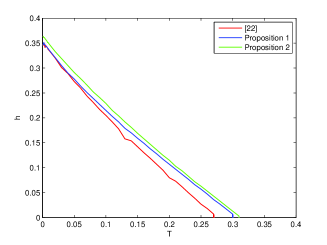
Figure 1: Example 1: tradeoff curve between maximal allowable $T$ and $h$ for Propositions 1 and 2 compared with the result of [22]

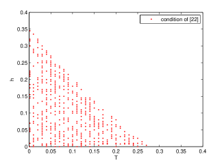
Figure 2: Example 1: stability region by the condition of [22]

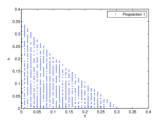
Figure 3: Example 1: stability region by Proposition 1

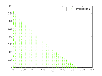
Figure 4: Example 1: stability region by Proposition 2

4 Extended Jensen summation inequalities with infinite sequences

The objective of this section is to present the discrete counterpart of the results obtained in Section 2 and to provide extended Jensen summation inequality with infinite sequences. We first introduce the following lemma for the discrete counterpart of the integral inequalities (4) and (5):

Lemma 2

Assume that there exist an $n\times n$ matrix $R\succ 0,$ a scalar function $M(i)\in{{\mathbb{R}}}^{+}$ and a vector function $x(i)\in{{\mathbb{R}}}^{n}$ such that the series concerned are convergent. Then the inequality

$$\begin{array}[]{lll}\sum_{i=0}^{+\infty}M(i)x^{T}(i)Rx(i)\\ \hskip 14.22636pt\geq M_{0}^{-1}\Big{[}\sum_{i=0}^{+\infty}M(i)x(i)\Big{]}^{T}R\Big{[}\sum_{i=0}^{+\infty}M(i)x(i)\Big{]},\end{array}$$ (36)

and its double summation extension

$$\begin{array}[]{lll}\sum_{i=0}^{+\infty}\sum_{j=k-i-h}^{k-1}M(i)x^{T}(j)Rx(j)\\ \hskip 14.22636pt\geq M_{1h}^{-1}\Big{[}\sum_{i=0}^{+\infty}\sum_{j=k-i-h}^{k-1}M(i)x(j)\Big{]}^{T}R\\ \hskip 28.45274pt\times\Big{[}\sum_{i=0}^{+\infty}\sum_{j=k-i-h}^{k-1}M(i)x(j)\Big{]},\end{array}$$ (37)

hold, where

$$\begin{array}[]{lll}M_{0}=\sum_{i=0}^{+\infty}M(i),\\ M_{1h}=\sum_{i=0}^{+\infty}(i+h)M(i).\end{array}$$ (38)

The proof of (36) and (37) follows from [22] by using sums instead of integrals and is therefore omitted here. By applying the arguments of Theorem 1 to the discrete case, we obtain the following theorem for the extended Jensen summation inequality with infinite sequences. Note that this result includes (36) as a special case and that the generalization of (37) can be done by the same approach as exploited in Theorem 2.

Theorem 3

For a given $n\times n$ matrix $R\succ 0,$ scalar functions $M(i):$ ${\mathbb{Z}}^{+}\to{{\mathbb{R}}}^{+},$ $g(i):$ ${\mathbb{Z}}^{+}\to{{\mathbb{R}}}$ and a vector function $x(i):$ ${\mathbb{Z}}^{+}\to{{\mathbb{R}}}^{n},$ assume that the series concerned are well defined and $\sum_{i=0}^{+\infty}M(i)g(i)=0$ with $g(i)$ not identically zero. Then the following inequality holds:

$$\begin{array}[]{ll}\sum_{i=0}^{+\infty}M(i)x^{T}(i)Rx(i)\\ \hskip 11.38092pt\geq M_{0}^{-1}\Big{[}\sum_{i=0}^{+\infty}M(i)x(i)\Big{]}^{T}R\Big{[}\sum_{i=0}^{+\infty}M(i)x(i)\Big{]}\\ \hskip 22.76228pt+\Big{[}\sum_{i=0}^{+\infty}M(i)g^{2}(i)\Big{]}^{-1}\Pi^{T}R\Pi\end{array}$$ (39)

with $M_{0}$ given by (38) and

$$\begin{array}[]{ll}\Pi=\sum_{i=0}^{+\infty}M(i)g(i)x(i).\end{array}$$ (40)

Proof: See Appendix B.

In order to apply Theorem 3 to the stability analysis of time-delay systems, we take

$$\begin{array}[]{ll}g(v)=c(M_{0}v-M_{1}),\ \ c\in{\mathbb{R}}\backslash\{0\},\ \ v\in{\mathbb{Z}}^{+},\end{array}$$ (41)

such that $\sum_{i=0}^{+\infty}M(i)g(i)=0$ is satisfied, where

$$\begin{array}[]{ll}M_{1}=\sum_{i=0}^{+\infty}iM(i).\end{array}$$ (42)

Hence, we have

$$\begin{array}[]{ll}\sum_{i=0}^{+\infty}M(i)g^{2}(i)=c^{2}\sum_{i=0}^{+\infty}M(i)(M_{0}i-M_{1})^{2}\\ \hskip 76.82234pt=c^{2}(M_{0}^{2}M_{2}-M_{0}M_{1}^{2}),\\ \Pi=\sum_{i=0}^{+\infty}M(i)g(i)x(i)\\ \hskip 11.38092pt=c\Big{[}M_{0}\sum_{i=0}^{+\infty}iM(i)x(i)-M_{1}\sum_{i=0}^{+\infty}M(i)x(i)\Big{]},\end{array}$$ (43)

where

$$\begin{array}[]{ll}M_{2}=\sum_{i=0}^{+\infty}i^{2}M(i).\end{array}$$ (44)

From (41) and (43), Theorem 3 is reduced to the following corollary, which will be employed in the next section for the stability analysis of discrete-time systems with poisson-distributed delays.

Corollary 3

Given an $n\times n$ matrix $R\succ 0,$ a scalar function $M(i):$ ${\mathbb{Z}}^{+}\to{{\mathbb{R}}}^{+}$ and a vector function $x(i):$ ${\mathbb{Z}}^{+}\to{{\mathbb{R}}}^{n}$ such that the series concerned are well defined, the following inequality holds:

$$\begin{array}[]{ll}\sum_{i=0}^{+\infty}M(i)x^{T}(i)Rx(i)\\ \hskip 11.38092pt\geq M_{0}^{-1}\Big{[}\sum_{i=0}^{+\infty}M(i)x(i)\Big{]}^{T}R\Big{[}\sum_{i=0}^{+\infty}M(i)x(i)\Big{]}\\ \hskip 22.76228pt+\Big{(}M_{2}-{M_{1}^{2}\over M_{0}}\Big{)}^{-1}\tilde{\Pi}^{T}R\tilde{\Pi},\end{array}$$ (45)

where $M_{0},$ $M_{1}$ and $M_{2}$ are given by (38), (42) and (44), respectively, and

$$\begin{array}[]{ll}\tilde{\Pi}={M_{1}\over M_{0}}\sum_{i=0}^{+\infty}M(i)x(i)-\sum_{i=0}^{+\infty}iM(i)x(i).\end{array}$$

5 Stability analysis of discrete-time systems with poisson-distributed delays

In this section, we will demonstrate the efficiency of the extended Jensen summation inequality (45) through the stability analysis of linear discrete-time systems with poisson-distributed delays. Consider the following system:

$$\begin{array}[]{lll}x(k+1)=Ax(k)+A_{1}\sum_{\tau=0}^{+\infty}p(\tau)x(k-\tau),\ \ k\in{{\mathbb{Z}}}^{+},\end{array}$$ (46)

where $x(k)\in{{\mathbb{R}}}^{n}$ is the state vector, the system matrices $A$ and $A_{1}$ are constant with appropriate dimensions. We do not allow $A$ and $A+A_{1}$ to be Schur stable. The initial condition is given as $\operatorname{col}\{x(0),x(-1),x(-2),\dots\}=\operatorname{col}\{\phi(0),\phi(-1),\phi(-2),\dots\}.$ The function $p(v),$ $v\in{{\mathbb{Z}}}^{+},$ is a poisson distribution with a fixed time gap $h\in{{\mathbb{Z}}}^{+}$:

$$\begin{array}[]{lll}p(v)=\left\{\begin{array}[]{cl}\frac{e^{-\lambda}\lambda^{v-h}}{(v-h)!}&v\geq h,\\ 0&v<h,\end{array}\right.\end{array}$$

where $\lambda>0$ is a parameter of the distribution. The mean value of $p$ is $h+\lambda$. Due to the fact that

$$\begin{array}[]{lll}\sum_{\tau=0}^{+\infty}p(\tau)x(k-\tau)&=&\sum_{\tau=h}^{+\infty}p(\tau)x(k-\tau)\\ &=&\sum_{\theta=0}^{+\infty}p(\theta+h)x(k-\theta-h),\end{array}$$

we arrive at the equivalent system:

$$\begin{array}[]{lll}x(k+1)\!=\!Ax(k)\!+\!A_{1}\sum_{\tau=0}^{+\infty}{\rm P}(\tau)x(k-\!\tau\!-h),\ k\in{{\mathbb{Z}}}^{+},\end{array}$$ (47)

where ${\rm P}(\tau)=\frac{e^{-\lambda}\lambda^{\tau}}{\tau!}$. We next derive LMI conditions for the asymptotic stability of (47) via a direct Lyapunov method.

Denoting

$$\begin{array}[]{lll}f(k)=\sum_{\tau=0}^{+\infty}{\rm P}(\tau)x(k-\tau-h),\ \ k\in{{\mathbb{Z}}}^{+},\end{array}$$

the system (47) can be transformed into the following augmented form

$$\begin{array}[]{lll}x(k+1)=Ax(k)+A_{1}f(k),\\ f(k+1)=\sum_{\tau=0}^{+\infty}\frac{e^{-\lambda}\lambda^{\tau}}{\tau!}x(k+1-\tau-h)\\ \hskip 8.5359pt=e^{-\lambda}x(k+1-h)+\sum_{\tau=1}^{+\infty}\frac{e^{-\lambda}\lambda^{\tau}}{\tau!}x(k+1-\tau-h)\\ \hskip 8.5359pt=e^{-\lambda}x(k+1-h)+\sum_{\tau=0}^{+\infty}\frac{e^{-\lambda}\lambda^{\tau+1}}{(\tau+1)!}x(k-\tau-h)\\ \hskip 8.5359pt=e^{-\lambda}Ax(k-h)+e^{-\lambda}A_{1}f(k-h)\\ \hskip 14.22636pt+\sum_{\tau=0}^{+\infty}{\rm Q}(\tau)x(k-\tau-h),\end{array}$$ (48)

where ${\rm Q}(\tau)=\frac{e^{-\lambda}\lambda^{\tau+1}}{(\tau+1)!}$. It is noted that the augmented system (48) has not only distributed but also discrete delays. This is different from augmented system (24) for the case of gamma-distributed delays. Moreover, we find that

$$\begin{array}[]{lll}\sum_{i=0}^{+\infty}(i+h){\rm P}(i)=\lambda+h,\\ \sum_{i=0}^{+\infty}{\rm Q}(i)=1-e^{-\lambda},\\ \sum_{i=0}^{+\infty}i{\rm Q}(i)=\lambda-1+e^{-\lambda}\stackrel{{\scriptstyle\Delta}}{{=}}{\bar{\rm Q}}_{1},\\ \sum_{i=0}^{+\infty}i^{2}{\rm Q}(i)=\lambda^{2}-\lambda+1-e^{-\lambda}\stackrel{{\scriptstyle\Delta}}{{=}}{\bar{\rm Q}}_{2},\\ \sum_{i=0}^{+\infty}(i+h){\rm Q}(i)=\lambda\!+\!(1-e^{-\lambda})(h\!-\!1)\stackrel{{\scriptstyle\Delta}}{{=}}{\bar{\rm Q}}_{1h}.\end{array}$$ (49)

Consider system (48) with both distributed and discrete delays. The stability analysis will be based on the following discrete-time LKF:

$$\begin{array}[]{lll}V(k)\!=\!{\hat{x}}^{T}(k)\hat{W}\hat{x}(k)\!+\!\sum_{i=1}^{2}\Big{[}V_{G_{i}}(k)+V_{H_{i}}(k)+V_{S_{i}}(k)\Big{]},\\ V_{G_{1}}(k)=\sum_{i=0}^{+\infty}\sum_{s=k-i-h}^{k-1}{\rm P}(i)x^{T}(s)G_{1}x(s),\\ V_{H_{1}}(k)=\sum_{i=0}^{+\infty}\sum_{j=1}^{i+h}\sum_{s=k-j}^{k-1}{\rm P}(i)\eta_{1}^{T}(s)H_{1}\eta_{1}(s),\\ V_{G_{2}}(k)=\sum_{i=0}^{+\infty}\sum_{s=k-i-h}^{k-1}{\rm Q}(i)x^{T}(s)G_{2}x(s),\\ V_{H_{2}}(k)=\sum_{i=0}^{+\infty}\sum_{j=1}^{i+h}\sum_{s=k-j}^{k-1}{\rm Q}(i)\eta_{1}^{T}(s)H_{2}\eta_{1}(s),\\ V_{S_{1}}(k)=\sum_{s=k-h}^{k-1}x^{T}(s)S_{1}x(s)\\ \hskip 42.67912pt+h\sum_{j=-h}^{-1}\sum_{s=k+j}^{k-1}\eta_{1}^{T}(s)R_{1}\eta_{1}(s),\\ V_{S_{2}}(k)=\sum_{s=k-h}^{k-1}f^{T}(s)S_{2}f(s)\\ \hskip 42.67912pt+h\sum_{j=-h}^{-1}\sum_{s=k+j}^{k-1}\eta_{2}^{T}(s)R_{2}\eta_{2}(s),\end{array}$$

where $\hat{W}\succ 0,$ $G_{i}\succ 0,$ $H_{i}\succ 0,$ $S_{i}\succ 0,$ $R_{i}\succ 0,$ $i=1,2,$ and

$$\begin{array}[]{lll}\hat{x}(k)=\operatorname{col}\{x(k),\ f(k)\},\\ \eta_{1}(k)=x(k+1)-x(k),\\ \eta_{2}(k)=f(k+1)-f(k).\end{array}$$

Here the last two terms $V_{S_{1}}(k)$ and $V_{S_{2}}(k)$ are added to compensate the delayed terms $x(k-h)$ and $f(k-h)$ of (48), respectively. Therefore, for system (48) with $h=0,$ the terms $V_{S_{1}}(k)$ and $V_{S_{2}}(k)$ are not necessary. From standard arguments, we arrive at the following result for the asymptotic stability of (48):

Proposition 3

Given a real scalar $\lambda>0$ and an integer $h\geq 0,$ assume that there exist $2n\times 2n$ positive definite matrix $\hat{W}$ and $n\times n$ positive definite matrices $G_{i},$ $H_{i},$ $S_{i},$ $R_{i},$ $i=1,2,$ such that the following LMI is satisfied:

$$\begin{array}[]{lll}\hat{\Xi}&=&\hat{\Sigma}\!+\!\hat{F}_{0}^{T}\hat{W}\hat{F}_{0}\!-\!\hat{F}_{1}^{T}\hat{W}\hat{F}_{1}-(\lambda+h)^{-1}\hat{F}_{12}^{T}H_{1}\hat{F}_{12}\\ &&+\hat{F}_{01}^{T}[(\lambda\!+\!h)H_{1}+{\bar{\rm Q}}_{1h}H_{2}+h^{2}R_{1}]\hat{F}_{01}\\ &&+h^{2}\hat{F}_{02}^{T}R_{2}\hat{F}_{02}-{{\bar{\rm Q}}_{1h}}^{-1}\hat{F}_{15}^{T}H_{2}\hat{F}_{15}-\hat{F}_{13}^{T}R_{1}\hat{F}_{13}\\ &&-\hat{F}_{24}^{T}R_{2}\hat{F}_{24}-\Big{(}\bar{Q}_{2}-{\bar{Q}_{1}^{2}\over 1-e^{-\lambda}}\Big{)}^{-1}\hat{F}_{25}^{T}G_{2}\hat{F}_{25}\prec 0,\end{array}$$ (50)

where $\bar{Q}_{1},$ $\bar{Q}_{2}$ and $\bar{Q}_{1h}$ are given by (49), $\hat{\Sigma}={\rm diag}\{S_{1}+G_{1}+(1-e^{-\lambda})G_{2},-G_{1}+S_{2},-S_{1},-S_{2},-(1-e^{-\lambda})^{-1}G_{2}\}$,

$$\begin{array}[]{lll}\hat{F}_{0}=\left[\begin{array}[]{ccccc}A&A_{1}&0&0&0\\ 0&0&e^{-\lambda}A&e^{-\lambda}A_{1}&I\end{array}\right],\\ \hat{F}_{1}=\left[\begin{array}[]{ccccc}I&0&0&0&0\\ 0&I&0&0&0\end{array}\right],\ \hat{F}_{01}=[A\!-\!I\ A_{1}\ 0\ 0\ 0],\\ \hat{F}_{02}=[0\ -\!I\ \ e^{-\lambda}A\ \ e^{-\lambda}A_{1}\ \ I],\ \hat{F}_{12}=[I\ -\!I\ 0\ 0\ 0],\\ \hat{F}_{13}=[I\ 0\ -\!I\ 0\ 0],\ \hat{F}_{15}=[(1-e^{-\lambda})I\ 0\ 0\ 0\ -\!I],\\ \hat{F}_{24}=[0\ I\ 0\ -\!I\ 0],\ \hat{F}_{25}=[0\ -\lambda I\ 0\ 0\ ({\bar{Q}_{1}\over 1-e^{-\lambda}}+1)I].\end{array}$$

Then the system (48) is asymptotically stable.

Proof: Define

$$\begin{array}[]{lll}q(k)=\sum_{\tau=0}^{+\infty}{\rm Q}(\tau)x(k-\tau-h),\\ \xi(k)=\operatorname{col}\{x(k),f(k),x(k-h),f(k-h),q(k)\}.\end{array}$$

By taking difference of $V(k)$ along (48) and applying Jensen inequalities with finite sequences (see e.g., Chapter 6 of [3]), we have

$$\begin{array}[]{lll}{\hat{x}}^{T}(k+1)\hat{W}\hat{x}(k+1)-{\hat{x}}^{T}(k)\hat{W}\hat{x}(k)\\ =\xi^{T}(k)[\hat{F}_{0}^{T}\hat{W}\hat{F}_{0}-\hat{F}_{1}^{T}\hat{W}\hat{F}_{1}]\xi(k)\end{array}$$ (51)

and

$$\begin{array}[]{lll}\sum_{i=1}^{2}\Big{[}V_{G_{i}}(k+1)+V_{H_{i}}(k+1)+V_{S_{i}}(k+1)\\ \hskip 34.14322pt-V_{G_{i}}(k)-V_{H_{i}}(k)-V_{S_{i}}(k)\Big{]}\\ =\xi^{T}(k)\Big{[}\hat{\Sigma}+\hat{F}_{01}^{T}[(\lambda+h)H_{1}+{\bar{\rm Q}}_{1h}H_{2}+h^{2}R_{1}]\hat{F}_{01}\\ \hskip 39.83368pt-(\lambda+h)^{-1}\hat{F}_{12}^{T}H_{1}\hat{F}_{12}+h^{2}\hat{F}_{02}^{T}R_{2}\hat{F}_{02}\\ \hskip 39.83368pt-\hat{F}_{13}^{T}R_{1}\hat{F}_{13}-\hat{F}_{24}^{T}R_{2}\hat{F}_{24}\Big{]}\xi(k)\\ \hskip 14.22636pt+(1-e^{-\lambda})^{-1}q^{T}(k)G_{2}q(k)\\ \hskip 14.22636pt-\sum_{i=0}^{+\infty}{\rm Q}(i)x^{T}(k-i-h)G_{2}x(k-i-h)\\ \hskip 14.22636pt-\sum_{i=0}^{+\infty}\sum_{s=k-i-h}^{k-1}{\rm Q}(i)\eta_{1}^{T}(s)H_{2}\eta_{1}(s).\end{array}$$ (52)

Applying the generalized Jensen inequality (45) with infinite sequences, we obtain

$$\begin{array}[]{lll}-\sum_{i=0}^{+\infty}{\rm Q}(i)x^{T}(k-i-h)G_{2}x(k-i-h)\\ \leq-(1-e^{-\lambda})^{-1}q^{T}(k)G_{2}q(k)\\ \quad-\Big{(}\bar{Q}_{2}-{\bar{Q}_{1}^{2}\over 1-e^{-\lambda}}\Big{)}^{-1}\Big{[}\Big{(}{\bar{Q}_{1}\over 1-e^{-\lambda}}\!+\!1\Big{)}q(k)\!-\!\lambda f(k)\Big{]}^{T}\!G_{2}\\ \hskip 19.91684pt\times\Big{[}\Big{(}{\bar{Q}_{1}\over 1-e^{-\lambda}}+1\Big{)}q(k)-\lambda f(k)\Big{]}\\ =-(1-e^{-\lambda})^{-1}q^{T}(k)G_{2}q(k)\\ \hskip 11.38092pt-\Big{(}\bar{Q}_{2}-{\bar{Q}_{1}^{2}\over 1-e^{-\lambda}}\Big{)}^{-1}\xi^{T}(k)\hat{F}_{25}^{T}G_{2}\hat{F}_{25}\xi(k).\end{array}$$ (53)

Furthermore, the application of (37) leads to

$$\begin{array}[]{lll}-\sum_{i=0}^{+\infty}\sum_{s=k-i-h}^{k-1}{\rm Q}(i)\eta_{1}^{T}(s)H_{2}\eta_{1}(s)\\ \leq\!-\Big{[}\!\sum_{i=0}^{+\infty}(i\!+\!h){\rm Q}(i)\Big{]}^{-1}\!\Big{[}\!\sum_{i=0}^{+\infty}\!\sum_{s=k-i-h}^{k-1}\!{\rm Q}(i)\eta_{1}(s)\Big{]}^{T}\!\!\!H_{2}\\ \hskip 14.22636pt\times\Big{[}\sum_{i=0}^{+\infty}\sum_{s=k-i-h}^{k-1}{\rm Q}(i)\eta_{1}(s)\Big{]}\\ =-{{\bar{\rm Q}}_{1h}}^{-1}[(1\!-\!e^{-\lambda})x(k)\!-\!q(k)]^{T}H_{2}[(1\!-\!e^{-\lambda})x(k)\!-\!q(k)]\\ =-{{\bar{\rm Q}}_{1h}}^{-1}\xi^{T}(k)\hat{F}_{15}^{T}H_{2}\hat{F}_{15}\xi(k).\end{array}$$ (54)

Therefore, (51)–(54) yield $\Delta V(k)=V(k+1)-V(k)\leq\xi^{T}(k)\hat{\Xi}\xi(k).$ Then if (50) holds for given scalars $\lambda>0$ and $h\geq 0$, the system (48) is asymptotically stable.

Remark 4

The LMI condition in Proposition 3 is derived by employing the generalized Jensen inequality (45). The system (48) can be alternatively analyzed by inequality (36). In this case, (53) is reduced to:

$$\begin{array}[]{lll}-\sum_{i=0}^{+\infty}{\rm Q}(i)x^{T}(k-i-h)G_{2}x(k-i-h)\\ \hskip 8.5359pt\leq-(1-e^{-\lambda})^{-1}q^{T}(k)G_{2}q(k).\end{array}$$

It yields $\hat{\Xi}_{|\hat{F}_{25}=0}\prec 0$, which is more conservative than the condition proposed in Proposition 3 since the matrix $-\Big{(}\bar{Q}_{2}-{\bar{Q}_{1}^{2}\over 1-e^{-\lambda}}\Big{)}^{-1}\hat{F}_{25}^{T}G_{2}\hat{F}_{25}$ of (50) is negative definite.

Remark 5

Both conditions in Proposition 3 and Remark 4 are derived by the use of inequality (37). It is worth noting that the results could be further improved (in the $(\lambda,h)$ plane preserving the stability) by the discrete counterpart of Theorem 2.

5.1 Example 2

Consider the linear discrete-time system (46) with

$$A=\left[\begin{array}[]{cc}-0.5&0\\ 0&1\end{array}\right]\ \ \text{and}\ \ A_{1}=\left[\begin{array}[]{cc}-0.5&0.8\\ 0.5&-0.2\end{array}\right].$$

Here neither $A$ nor $A+A_{1}$ is Schur stable. For $h=0$ the values of $\lambda$ that guarantee the asymptotic stability of the system by Remark 4 and Proposition 3 are shown in Fig. 5, where we can see that the results achieved by Proposition 3 are less conservative than those obtained by Remark 4. It is noted that Proposition 3 and Remark 4 possess the same number $\{5n^{2}+4n\}_{n=2}=28$ of variables.

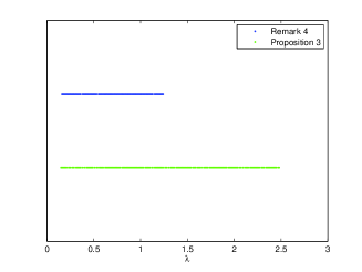
Figure 5: Example 2: stabilizing values of $\lambda$

6 Conclusions

In this paper, we have provided extended Jensen integral inequalities. For the discrete counterpart we have generalized Jensen summation inequality. Applications to the stability analysis of linear continuous-time systems with gamma-distributed delays and linear discrete-time systems with poisson-distributed delays demonstrated the advantages of these generalized inequalities. In both cases, the considered infinite distributed delays with a gap have stabilizing effects. The future research may include other applications of these developed inequalities.

Appendix A

Proof of Theorem 2 Following the proof of Theorem 1, we define a function $f(r,u)$ for all $u\in[0,+\infty)$, $r\in[t-u-h,t]$ by $f(r,u)=\hat{f}(r,u)-\sqrt{K(u)}g(r)\hat{\Theta},$ where $\hat{\Theta}\in{\mathbb{R}}^{n}$ is a constant vector to be defined and $\hat{f}(r,u)=\sqrt{K(u)}\Big{[}\omega(r)-K_{1h}^{-1}\int_{0}^{+\infty}\int_{t-\theta-h}^{t}K(\theta)\omega(s)dsd\theta\Big{]}$ with $K_{1h}$ given by (17). Since $R\succ 0$ we have

$$\begin{array}[]{llll}0&\leq&\int_{0}^{+\infty}\int_{t-\theta-h}^{t}f^{T}(s,\theta)Rf(s,\theta)dsd\theta\\ &=&\int_{0}^{+\infty}\int_{t-\theta-h}^{t}\hat{f}^{T}(s,\theta)R\hat{f}(s,\theta)dsd\theta\\ &&+\Big{[}2K_{1h}^{-1}\hat{\Theta}^{T}R\int_{0}^{+\infty}\int_{t-\theta-h}^{t}K(\theta)\omega(s)dsd\theta\Big{]}\\ &&\quad\ \times\int_{0}^{+\infty}\int_{t-\theta-h}^{t}K(\theta)g(s)dsd\theta\\ &&+\Big{[}\int_{0}^{+\infty}\int_{t-\theta-h}^{t}K(\theta)g^{2}(s)dsd\theta\Big{]}\hat{\Theta}^{T}R\hat{\Theta}\\ &&-2\hat{\Theta}^{T}R\int_{0}^{+\infty}\int_{t-\theta-h}^{t}K(\theta)g(s)\omega(s)dsd\theta,\end{array}$$

Rewriting the last two terms as sum of squares together with $\int_{0}^{+\infty}\int_{t-\theta-h}^{t}K(\theta)g(s)dsd\theta=0$ leads to

$$\begin{array}[]{llll}\int_{0}^{+\infty}\int_{t-\theta-h}^{t}K(\theta)\omega^{T}(s)R\omega(s)dsd\theta\\ \hskip 28.45274pt\geq K_{1h}^{-1}\int_{0}^{+\infty}\int_{t-\theta-h}^{t}K(\theta)\omega^{T}(s)dsd\theta R\\ \hskip 28.45274pt\times\int_{0}^{+\infty}\int_{t-\theta-h}^{t}K(\theta)\omega(s)dsd\theta\\ \hskip 14.22636pt+\Big{[}\int_{0}^{+\infty}\int_{t-\theta-h}^{t}K(\theta)g^{2}(s)dsd\theta\Big{]}^{-1}\Sigma^{T}R\Sigma\\ \hskip 14.22636pt-\Big{[}\int_{0}^{+\infty}\int_{t-\theta-h}^{t}K(\theta)g^{2}(s)dsd\theta\Big{]}[\hat{\Theta}-\hat{\Upsilon}]^{T}R[\hat{\Theta}-\hat{\Upsilon}],\end{array}$$ (55)

where $\Sigma$ is given by (18) and

$$\begin{array}[]{llll}\hat{\Upsilon}=\Big{[}\int_{0}^{+\infty}\int_{t-\theta-h}^{t}K(\theta)g^{2}(s)dsd\theta\Big{]}^{-1}\\ \hskip 22.76228pt\times\int_{0}^{+\infty}\int_{t-\theta-h}^{t}K(\theta)g(s)\omega(s)dsd\theta.\end{array}$$

Then the inequality (55) with $\hat{\Theta}=\hat{\Upsilon}$ implies (17). This concludes the proof.

Appendix B

Proof of Theorem 3 Define a function $f(v)$ for all $v\in{\mathbb{Z}}^{+}$ by $f(v)=\tilde{f}(v)-\sqrt{M(v)}g(v)\tilde{\Theta},$ where $\tilde{\Theta}\in{\mathbb{R}}^{n}$ is a constant vector to be defined and $\tilde{f}(v)=\sqrt{M(v)}\Big{[}x(v)-M_{0}^{-1}\sum_{i=0}^{+\infty}M(i)x(i)\Big{]}$ with $M_{0}$ given by (38) . Then since $R\succ 0$ it follows that

$$\begin{array}[]{llll}0&\leq&\sum_{i=0}^{+\infty}f^{T}(i)Rf(i)\\ &=&\Big{[}2M_{0}^{-1}\tilde{\Theta}^{T}R\sum_{i=0}^{+\infty}M(i)x(i)\Big{]}\sum_{i=0}^{+\infty}M(i)g(i)\\ &&+\sum_{i=0}^{+\infty}\tilde{f}^{T}(i)R\tilde{f}(i)\\ &&+\Big{[}\sum_{i=0}^{+\infty}M(i)g^{2}(i)\Big{]}\tilde{\Theta}^{T}R\tilde{\Theta}\\ &&-2\tilde{\Theta}^{T}R\sum_{i=0}^{+\infty}M(i)g(i)x(i).\end{array}$$

Representing the last two terms as sum of squares together with $\sum_{i=0}^{+\infty}M(i)g(i)=0$ yields

$$\begin{array}[]{llll}\sum_{i=0}^{+\infty}M(i)x^{T}(i)Rx(i)\\ \hskip 11.38092pt\geq M_{0}^{-1}\Big{[}\sum_{i=0}^{+\infty}M(i)x(i)\Big{]}^{T}R\Big{[}\sum_{i=0}^{+\infty}M(i)x(i)\Big{]}\\ \hskip 17.07182pt+\Big{[}\sum_{i=0}^{+\infty}M(i)g^{2}(i)\Big{]}^{-1}\Pi^{T}R\Pi\\ \hskip 17.07182pt-\Big{[}\sum_{i=0}^{+\infty}M(i)g^{2}(i)\Big{]}[\tilde{\Theta}-\tilde{\Upsilon}]^{T}R[\tilde{\Theta}-\tilde{\Upsilon}],\end{array}$$ (56)

where $\Pi$ is given by (40) and

$$\tilde{\Upsilon}=\Big{[}\sum_{i=0}^{+\infty}M(i)g^{2}(i)\Big{]}^{-1}\sum_{i=0}^{+\infty}M(i)g(i)x(i).$$

The choice of $\tilde{\Theta}=\tilde{\Upsilon}$ results in the maximum of the right-hand side of (56) and thus (39). This concludes the proof.

References

• [1] Y. Ariba and F. Gouaisbaut. Construction of Lyapunov-Krasovskii functional for time-varying delay systems. In Proceedings of the 47th IEEE Conference on Decision and Control, Cancun, Mexico, December 2008.
• [2] C. Briat. Convergence and equivalence results for the Jensen’s inequality–application to time-delay and sampled-data systems. IEEE Transactions on Automatic Control, 56(7):1660–1665, 2011.
• [3] E. Fridman. Introduction to Time-Delay Systems. Birkhäuser, 2014.
• [4] E. Fridman and U. Shaked. Delay-dependent stability and ${H}_{\infty}$ control: constant and time-varying delays. International Journal of Control, 76(1):48–60, 2003.
• [5] E. Fridman, U. Shaked, and K. Liu. New conditions for delay-derivative-dependent stability. Automatica, 45(11):2723–2727, 2009.
• [6] D. Gross, J. Shortle, J. Thompson, and C. Harris. Fundamentals of queueing theory. John Wiley & Sons, 2008.
• [7] K. Gu. An improved stability criterion for systems with distributed delays. International Journal of Robust and nonlinear control, 13(9):819–831, 2003.
• [8] K. Gu, V. Kharitonov, and J. Chen. Stability of Time-Delay Systems. Birkhäuser, Boston, 2003.
• [9] V.B. Kolmanovskii and J.P. Richard. Stability of some linear systems with delays. IEEE Transactions on Automatic Control, 44(5):984–989, 1999.
• [10] S.A. Kotsopoulos and K. Loannou. Handbook of Research on Heterogeneous Next Generation Networking: Innovations and Platforms. IGI Global, 2008.
• [11] K. Liu and E. Fridman. Wirtinger’s inequality and Lyapunov-based sampled-data stabilization. Automatica, 48(1):102–108, 2012.
• [12] K. Liu and E. Fridman. Delay-dependent methods and the first delay interval. Systems & Control Letters, 64(1):57–63, 2014.
• [13] Y.R. Liu, Z.D. Wang, J.L. Liang, and X.H. Liu. Synchronization and state estimation for discrete-time complex networks with distributed delays. IEEE Transactions on Systems, Man, and Cybernetics, Part B: Cybernetics, 38(5):1314–1325, 2008.
• [14] C.I. Morarescu, S.I. Niculescu, and K. Gu. Stability crossing curves of shifted gamma-distributed delay systems. SIAM Journal on Applied Dynamical Systems, 6(2):475–493, 2007.
• [15] S.I. Niculescu. Delay Effects on Stability: A Robust Control Approach. Springer-Verlag, Berlin, 2001.
• [16] P.G. Park, W.I. Lee, and S.Y. Lee. Auxiliary function-based integral inequalities for quadratic functions and their applications to time-delay systems. Journal of the Franklin Institute, 352(4):1378–1396, 2015.
• [17] J.P. Richard. Time-delay systems: An overview of some recent advances and open problems. Automatica, 39(10):1667–1694, 2003.
• [18] A. Saleh and R. Valenzuela. A statistical model for indoor multipath propagation. IEEE Journal on Selected Areas in Communications, 5(2):128–137, 1987.
• [19] A. Seuret and F. Gouaisbaut. On the use of the Wirtinger inequalities for time-delay systems. In Proceedings of the 10th IFAC workshop on time-delay systems, Boston, MA, USA, 2012.
• [20] A. Seuret and F. Gouaisbaut. Wirtinger-based integral inequality: application to time-delay systems. Automatica, 49(9):2860–2866, 2013.
• [21] A. Seuret, F. Gouaisbaut, and E. Fridman. Stability of discrete-time systems with time-varying delays via a novel summation inequality. IEEE Transactions on Automatic Control, 60(10):2740–2745, 2015.
• [22] O. Solomon and E. Fridman. New stability conditions for systems with distributed delays. Automatica, 49(11):3467–3475, 2013.
• [23] O. Solomon and E. Fridman. Stability and passivity analysis of semilinear diffusion PDEs with time-delays. International Journal of Control, 88(1):180–192, 2015.
• [24] J. Sun, G. Liu, and J. Chen. Delay-dependent stability and stabilization of neutral time-delay systems. International Journal of Robust and Nonlinear Control, 19(12):1364–1375, 2009.
• [25] Z.G. Wu, P. Shi, H.Y. Su, and J. Chu. Reliable control for discrete-time fuzzy systems with infinite-distributed delay. IEEE Transactions on Fuzzy Systems, 20(1):22–31, 2012.
• [26] Y.Q. Xia and Y.M. Jia. Robust control of state delayed systems with polytopic type uncertainties via parameter-dependent Lyapunov functionals. Systems & Control Letters, 50(3):183–193, 2003.