Maximizing the hyperpolarizability of 1D potentials with multiple electrons

Abstract

We optimize the first and second intrinsic hyperpolarizabilities for a 1D piecewise linear potential dressed with Dirac delta functions for $N$ non-interacting electrons. The optimized values fall rapidly for $N>1$, but approach constant values of $\beta_{int}=0.40$, $\gamma_{int}^{+}=0.16$ and $\gamma_{int}^{-}=-0.061$ above $N\gtrsim 8$. These apparent bounds are achieved with only 2 parameters with more general potentials achieving no better value. In contrast to previous studies, analysis of the hessian matrices of $\beta_{int}$ and $\gamma_{int}$ taken with respect to these parameters shows that the eigenvectors are well aligned with the basis vectors of the parameter space, indicating that the parametrization was well-chosen. The physical significance of the important parameters is also discussed.

I Introduction

Nonlinear optical materials are the active constituent for many applications such as light modulators, contrast agents for medical imaging and therapy, optical solitons, phase conjugation mirrors and optical self-modulation. In each of these, the performance of the system is improved by using a material with a stronger nonlinear response, quantified by various nonlinear susceptibilities defined by expanding the induced polarization $P$ in a power series in the applied electric field,

$$P=\alpha E+\beta EE+\gamma EEE+O(\epsilon^{4}).$$ (1)

Here, $\alpha$ is the linear susceptibility familiar from dielectric materials; $\beta$ and $\gamma$ are the nonlinear susceptibilities and are referred to as the first and second hyperpolarizability respectively. These quantities are in general frequency-dependent tensors that depend on the electronic structure of the constituent molecules, their symmetry, ordering and the material in which they are embedded. In the present work we focus on the off-resonant molecular contribution. Much effort has been expended over the years in synthesizing new molecules with higher $\beta$ or $\gamma$. Comparisons between materials must be made carefully however, because these quantities increase trivially with the size of the molecule.

Important progress on developing suitable figures-of-merit for comparison was made by Kuzyk, who showed that fundamental quantum mechanics requires that $\beta$ and $\gamma$ for the off-resonant case are bounded by the inequalities,

$$\left|\beta\right| \leq\sqrt[3]{4}\left(\frac{e\hbar}{\sqrt{m}}\right)^{3}\frac{N^{3/2}}{E_{10}^{7/2}}\equiv\beta_{0}^{max},$$ (2)

$$\left(\frac{e\hbar}{\sqrt{m}}\right)^{4}\frac{N^{2}}{E_{10}^{5}}\leq \gamma \leq 4\left(\frac{e\hbar}{\sqrt{m}}\right)^{4}\frac{N^{2}}{E_{10}^{5}}\equiv\gamma_{0}^{max}$$ (3)

where $E_{10}$ is the difference between the ground and first excited state and $N$ is the number of electrons participating. From the maximum values $\beta_{0}^{max}$ and $\gamma_{0}^{max}$, one defines intrinsic hyperpolarizabilities,

$$\beta_{int}=\beta/\beta_{0}^{max},\ \gamma_{int}=\gamma/\gamma_{0}^{max}.$$ (4)

The intrinsic quantities have the property that they remain invariant under a simultaneous rescaling of energy and length,

$$x\to x^{\prime}E^{1/2},\ V(x)\to V^{\prime}(x^{\prime})E$$ (5)

and hence are useful quantities for comparing materials because they remove the irrelevant scaling with size. Analysis of extant materials following the derivation of the bounds in eq. (3) revealed that all of them fell short of the fundamental limits by more than an order of magnitude, an observation that has catalyzed a great deal of research over the past decade on how to create materials that approach these fundamental limits. The derivation of the bounds provides some guidance—for optimal $\beta$ and $\gamma$ only three states are assumed to significantly contribute to the hyperpolarizabilities and the optimum can be achieved by tuning the dipole transition matrix elements and energy level spacings—but does not construct an explicit molecule or potential that has these properties.

Subsequent work, thoroughly reviewed in Kuzyk et al. (2013) has attempted to determine whether these predictions are universal and to explicitly construct potentials that approach them. One approach has been to conduct Monte Carlo searches of Hamiltonians with arbitrary spectra and dipole transition elements to identify those with large $\beta_{int}$ and $\gamma_{int}$. The results support the three-state hypothesis, though the optima found in such calculations need not correspond to a local potential. To address this, several authors have numerically optimized the intrinsic hyperpolarizabilities with respect to the potential function for 1 electron, using various representations of the potential, including power lawsMossman and Kuzyk (2013), elementary functions with a superimposed Fourier seriesWatkins and Kuzyk (2012), piecewise linear potentialsAtherton et al. (2012); Burke et al. (2013) and quantum graphsLytel et al. (2013); Lytel and Kuzyk (2013); Lytel et al. (2014, 2015). The best potentials from these different studies possess hyperpolarizabilities within the bounds of eq. (3) with the best known values found of $\beta_{int}\sim 0.71$ and $\gamma_{int}\sim 0.60$ achieved in several studies with qualitatively different potentials. It has therefore been speculated that the fundamental limits may require exotic potentials and not be achievable with local potential functions. The effect of including multiple electrons on the optimized potentials has, however, received relatively little attention. Watkins and coworkers Watkins and Kuzyk (2011) found for $N=2$ electrons that the best intrinsic hyperpolarizabilities are somewhat lower than for the $N=1$ electron case, but even with electron-electron interactions included, the universal features identified in other studies remained the same.

In this paper, we apply the potential optimization technique to potentials with $N>2$ electrons that interact only through Pauli exclusion. This is a key step towards simulating realistic molecules. We find that the best values of $\beta_{int}$ and $\gamma_{int}$ fall off with increasing $N$ from the $N=1$ electron case, but rapidly converge to a universal value. The small number of parameters in our potentials allows a detailed exploration of the “landscape” of $\beta_{int}$ and $\gamma_{int}$ around the maximum. As in previous work, the hyperpolarizabilities are more sensitive to one parameter than the other. Dimensional and approximate analytical arguments allow us to provide physical interpretations of these two parameters in terms of the wavefunctions of the highest occupied molecular orbital.

The paper is organized as follows: in section II the choice of potential, calculation and optimization techniques are briefly reviewed; in section III we present results for $\beta_{int}$ and $\gamma_{int}$ separately together with some discussion of the implications of our results for identifying the features of potentials most important to the hyperpolarizabilities; brief conclusions are presented in section IV.

II Model

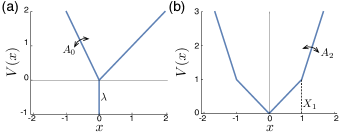
Figure 1: Schematics of the potential classes in which $\beta_{\mathrm{int}}$ and $\gamma_{\mathrm{int}}$ are optimized. (a) Asymmetric triangle will with a delta function at the center. The slope on the right side is fixed at $1$ while the slope of the side $A_{0}$ and the strength of the delta function $\alpha$ can be varied. $A_{0}$ can be fixed at 1 to study a symmetric 1-parameter potential. (b) a 2 parameter symmetric linear piecewise potential. The first slope to the right of the origin is fixed at 1. The position of the boundary between the first and second elements $X_{1}$ and the second slope $A_{2}$ can be varied. The left side of the potential is constrained to be the reflection of the right side.

Following a similar approach to that established in our earlier papersAtherton et al. (2012); Burke et al. (2013), we optimize $\beta_{int}$ and $\gamma_{int}$ with respect to the shape of a piecewise linear potential dressed with Dirac delta functions for $N$ electrons interacting only through Pauli exclusion. We perform this optimization for two carefully chosen potentials depicted in Fig. 1 as well as a more general potential. The first type is an asymmetric triangular well with a delta function at the center [fig. 1(a)],

$$V_{1}(x)=-\alpha\delta(x)+\begin{cases}-A_{0}x,&x<0\\ x&x\geq 0\end{cases},$$ (6)

parametrized by the left hand slope $A_{0}>0$ and the strength of the $\delta$-function $\alpha$. The effect of the $\delta$ function is to introduce a sudden change in the phase of the wavefunction. Lytel et al. Lytel et al. (2015) recently showed that the addition of a $\delta$ function to a 1D potential has an equivalent effect on the wavefunction to adding a side chain on a quantum graph. This correspondence suggests that 1D potentials dressed with $\delta$-functions could be engineered in molecules by the addition of appropriate side groups.

The second type of potential we consider, depicted in fig. 1(b), contains only linear elements defined for $x>0$,

$$V_{2}(x)=\begin{cases}x&0<x<X_{1}\\ A_{2}(x-X_{1})+X_{1}&x\geq X_{1}\end{cases},$$ (7)

and for $x<0$ defined by enforcing $\mathcal{P}$ symmetry, i.e. $V(-x)=V(x)$; this potential is specified by two parameters $X_{1}$ the position of the boundary between the two elements and $A_{2}$ the slope of the outermost element. These potentials were motivated by our results in Atherton et al. (2012); Burke et al. (2013) that only 2 parameters at most were important to the optimization of both $\beta_{int}$ and $\gamma_{int}$; they have been designed to achieve the known limits for $N=1$ electrons with residual flexibility. For example, we showed in Burke et al. (2013) that a triangular well with a $\delta$-function of variable strength at the center, i.e. taking the potential (6) and fixing $A_{0}=1$, was able to reach within $3\%$ of the upper bound for $\gamma_{int}$ with $\lambda$ as the only free parameter. The parametrization has also been chosen to eliminate variables irrelevant to $\beta_{int}$ and $\gamma_{int}$ associated with translations of the potential and rescalings of the form (5).

We also minimized $\beta_{int}$ for a piecewise linear potential with $m$ elements,

$$V(x)=\begin{cases}A_{0}x+B_{0}&x<x_{0}\\ A_{n}x+B_{n}&x_{n-1}<x<x_{n}\\ A_{m}x+B_{n}&x>x_{m-1}\end{cases},$$ (8)

with positions $x_{n}$ and slopes $A_{n}$ as the parameter set describing the potential. We used this potential in our earlier paper on maximizing $\beta_{int}$ for one electronAtherton et al. (2012). There are some necessary constraints on the parameters: the $x_{n}$ are strictly ascending; $x_{0}=0$ and $B_{0}=0$ with no loss of generality and $B_{1}=B_{0}$ with the remaining constants $B_{n}$ given by,

$$B_{n}=\sum_{m=1}^{n-1}(A_{m}-A_{m+1})x_{m}.$$ (9)

The energy scale associated with the potential is also fixed, as in the previous paper, by setting $A_{1}=1$. Having imposed these constraints, there remain $2N-1$ free parameters.

For each of these potentials, $\beta_{int}$ and $\gamma_{int}$ were calculated for $N$ electrons as follows: first, the Schrödinger equation is written for each segment as,

$$\left[-\frac{1}{2}\frac{d}{dx^{2}}+(A_{n}+\epsilon)x+B_{n}\right]\psi_{n}=E\psi_{n}$$ (10)

where $A_{n}$ and $B_{n}$ are the slope and offset in the $n$th segment and $\epsilon$ is the applied electric field. This can be solved analytically using the well-known Airy functions,

$$\psi_{n}(x) = C_{n}\text{Ai}\left[\frac{\sqrt[3]{2}\left(B_{n}-E+x\left(A_{n}+\epsilon\right)\right)}{\left(A_{n}+\epsilon\right)^{2/3}}\right]$$ (11)

$$+D_{n}\text{Bi}\left[\frac{\sqrt[3]{2}\left(B_{n}-E+x\left(A_{n}+\epsilon\right)\right)}{\left(A_{n}+\epsilon\right)^{2/3}}\right].$$

To solve for the coefficients $C_{n}$ and $D_{n}$ in each element, a set of boundary conditions are assembled at the edge of each element from the usual conditions, i.e.,

$$\psi_{n+1}(X_{n})-\psi_{n}(X_{n}) = 0$$ (12)

$$\psi^{\prime}_{n+1}(X_{n})-\psi_{n}^{\prime}(X_{n}) = \alpha_{n}\psi_{n}(X_{n})$$ (13)

where $\alpha_{n}$ is the strength of the delta function centered at $X_{n}$. The requirement that $\psi\to 0$ as $x\to\pm\infty$ eliminates two coefficients. The boundary conditions can be written as a set of linear equations,

$$W\cdot u=0$$ (14)

where $u$ is a vector comprised of the $C_{n}$ and $D_{n}$ coefficients and $W$ is a matrix that depends on $E$, $\epsilon$ and the parameters $A_{n}$ and $X_{n}$. The single electron energy levels $\lambda_{i}$ for the potential are determined by numerically finding the roots of,

$$\det W=0,$$ (15)

setting $\epsilon=0$. Having determined these, we construct the non-interacting $N$ electron ground state from the single electron states by successively filling the energy levels using the aufbau principle; we similarly determine the first excited state by promoting an electron from the highest occupied orbital to the lowest unoccupied orbital. In this work we focus only on even values of $N$, as this simplifies determining which electron to promote. The $N$-electron ground state energy $E_{0}$, and that of the first excited state $E_{1}$, are then determined by summing over the energies of the individual single electron energies,

$$E_{n}=\sum_{i}\nu{}_{i}^{n}\lambda_{i},$$ (16)

where $\nu_{i}^{n}$ is the occupation number for the $i$-th single electron level in the $n$-th multi-electron state.

The hyperpolarizabilities $\beta$ and $\gamma$ are obtained by differentiating the ground state energy as a function of $\epsilon$,

$$\beta\equiv\frac{1}{2}\frac{d^{3}E_{0}}{d\epsilon^{3}},\ \gamma\equiv\frac{1}{6}\frac{d^{4}E_{0}}{d\epsilon^{4}}.$$ (17)

The necessary derivatives can be related to the single-electron energy levels by differentiating (16) with respect to $\epsilon$. An important advantage of the piecewise linear potential is that the necessary derivatives of the single electron energy levels $\lambda_{i}$ are conveniently obtained by repeated differentiation of the determinant eq. (15) using the Jacobi formula,

$$\frac{d}{d\epsilon}\det W=\text{Tr}\left(\text{adj}W\cdot\frac{dW}{d\epsilon}\right),$$

where $\text{adj}W$ is the adjugate matrix of $W$, together with the chain rule,

$$\frac{dW}{d\epsilon}=\frac{\partial W}{\partial\epsilon}+\frac{\partial W}{\partial\lambda_{i}}\frac{d\lambda_{i}}{d\epsilon}.$$ (18)

To avoid repetition, formulae are available for these derivatives in references Atherton et al. (2012) and Burke et al. (2013). Having evaluated these derivatives, the intrinsic hyperpolarizabilities are easily calculated numerically and a program to do so was implemented in Mathematica 10. In subsequent sections, we present the optimized results as a function of $N$, together with the corresponding best potentials.

III Results

III.1 First hyperpolarizability

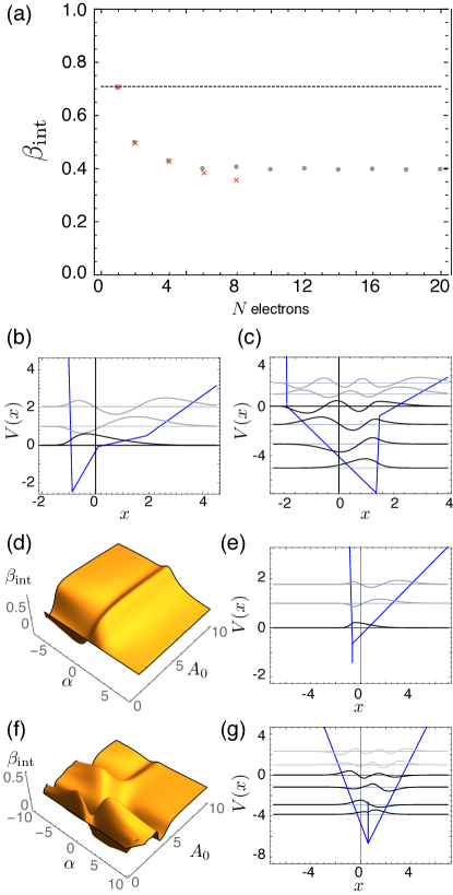
Figure 2: (a) Maximum $\beta_{\mathrm{int}}$ achieved in 2-parameter asymmetric $\delta$-function potential. Results for the asymmetric delta function potential are shown as grey circles; results for an arbitrary linear potential are shown as red crosses. The dashed line represents the largest values of $\beta_{\mathrm{int}}$ for one electron found to date. Optimized potential and wavefunctions for the arbitrary linear potential with (b) $N=2$ electrons and (c) $N=8$ electrons. For the asymmetric $\delta$-function potential and $N=2$, (d) the objective functions $\beta_{\mathrm{int}}$ plotted versus the $\delta$-function potential shape parameters $A_{0}$ and $\alpha$ and (e) the optimized potential and wavefunctions. Corresponding plots for $N=8$ electrons are shown in (f) and (g). For all subfigures, wavefunctions plotted in black are occupied in the ground state; those in grey correspond to the two lowest unoccupied states.

Value of $\beta_{int}$	Potential and wavefunctions	$A_{0}$	$\alpha$	Hessian Eigenvalues	Hessian Principal Eigenvector	$x_{nm}$	$X$	$E$
0.404 (100%)		1.334	-2.229	-6.84, -0.099	$\left(\begin{array}[]{c}0.999\\ 0.035\end{array}\right)$		0.573	0.500
-0.372 (96%)		1.227	1.928	7.70, 0.130	$\left(\begin{array}[]{c}0.999\\ 0.027\end{array}\right)$		0.570	0.500
0.370 (92%)		2.568	2.307	-1.24, -0.014	$\left(\begin{array}[]{c}0.986\\ -0.162\end{array}\right)$		0.569	0.523

Table 1: Asymmetric $\delta$-function potentials with locally optimal $\beta_{int}$. Results for each potential are shown columnwise: the value of $\beta_{int}$ , and the fraction of the globally optimum value; the potential and wavefunctions with black lines indicating states that are occupied and light gray lines indicated unoccupied states in the ground state configuration; optimized values of the parameters $A_{0}$ and $\delta$; the eigenvalues and eigenvectors of the Hessian matrix of $\beta_{int}$ with respect to the parameters; a plot of the dipole transition matrix $x_{nm}=\left\langle n\left|x\right|m\right\rangle$ with the Highest Occupied Molecular Orbital (HOMO) and Lowest Unoccupied Molecular Orbital (LUMO) indicated by H and L respectively, coloring described in the text; the energy ratio $E$ and dipole transition moment $X$ for the Kuzyk three-state model.

We optimized $\beta_{int}$ with respect to the parameters of the asymmetric $\delta$-function potential of eq. (6) as well as the more general piecewise linear potential with of eq. (8) with four linear elements and $6$ parameters. The number of linear elements was chosen because earlier work showed no improvement in $\beta_{int}$ after 6 parametersAtherton et al. (2012). The highest values found for increasing $N$ are displayed in fig. 2(a) for both of these. It is apparent that the best achievable result diminishes for $N>2$ but rapidly reaches a plateau of $\beta_{int}\sim 0.4$ and that both potentials give consistent results.

For $N\leq 8$ electrons, the two choices of potential give very consistent results, suggesting that we have indeed found a likely global optimum. For $N>8$ electrons, however, the optimization procedure failed to find a maximum of $\beta_{int}$ for the general linear potential that approached that of the asymmetric $\delta$-function potential. We speculate that this is because the number of local maxima increases with $N$; we shall show that this is true later for the more carefully chosen potentials at least. Because of this, we did not consider the general piecewise linear potential further but display the optimized potential and wavefunctions for $N=2$ and $N=8$ respectively in fig. 2(b) and (c). That these potentials achieve similar values of $\beta_{int}$ to the asymmetric $\delta$-function potentials, despite visually appearing very different, supports our conclusion in previous workAtherton et al. (2012) that $\beta_{int}$ is poorly determined in potential space with many irrelevant directions.

Due to the small parameter space of the asymmetric $\delta$-function potential, it is possible to directly visualize the objective function; this is displayed in fig. 2(d) for $N=1$ or 2 electrons (the magnitude is scaled by $2^{-1/2}$ for the $N=2$ electron case), with corresponding optimized potential and wavefunctions shown in fig. 2(e). The objective function for $N=8$ electrons and the optimized potential and wavefunctions are shown in fig. 2(f) and (g) respectively. It is immediately apparent that as $N$ increases, the objective function acquires additional local extrema.

For the $N=1$ case, the global optimum found is $\beta_{int}=0.701632$ at $A_{0}=35.283$ and $\alpha=1.1189$, which is only marginally short of the best known value of $\beta_{int}=0.708951$ found from optimizing many different classes of potential Atherton et al. (2012). The global maximum lies at the top of the long, narrow ridge viewed in fig. 2(d), a feature of the objective function that was also seen in earlier studies of more complicated potentials Atherton et al. (2012). Its presence implies that $\beta_{int}$ is much less sensitive to one of the parameters than the other, which can be quantified by computing the hessian matrix of $\beta_{int}$ with respect to the parameters,

$$h=\left(\begin{array}[]{cc}\frac{\partial^{2}}{\partial^{2}A_{0}}&\frac{\partial^{2}}{\partial A_{0}\partial\alpha}\\ \frac{\partial^{2}}{\partial A_{0}\partial\alpha}&\frac{\partial^{2}}{\partial^{2}\alpha}\end{array}\right),$$

and finding the eigenvalues and eigenvectors. These quantities respectively measure the curvature and principal directions of the objective function around the maximum. We previously used this technique in Atherton et al. (2012) to show that that while the best known value of $\beta_{int}=0.708951$ was obtained by optimizing a piecewise linear potential with 6 free parameters, in fact $\beta_{int}$ was effectively only sensitive to 2-3 parameters at the optimum. Here, the eigenvalues of the hessian evaluated at the global maximum of $\beta_{int}$ are $-0.32277$ and $-0.00066$ and the associated eigenvectors are $(0.00965,-0.99995)$ and $(0.99995,0.00965)$. Hence, $\beta_{int}$ is very sensitive to the value of $\alpha$, the second parameter and much less sensitive to the value of $A_{0}$; Since the eigenvectors are nearly parallel to basis vectors $(1,0)$ and $(0,1)$ in parameter space—as is visible from the orientation of the ridge in fig. 2(d)—it is clear that $\beta_{int}$ is sensitive to these features of the potential specifically, and not some combination of them. In contrast, the eigenvectors in Atherton et al. (2012) were not well aligned with the parameter space and so it was not possible to ascribe high $\beta_{int}$ to particular features of the potential. The design advice from this study is much clearer: to optimize $\beta_{int}$, create an asymmetric potential well with a steep wall on one side, i.e. set $A_{0}\gg 1$; then add an attractive group in the center and tune the strength of attraction, i.e. carefully adjust $\alpha$ as this largely determines $\beta_{int}$.

A similar analysis was applied to the multi-electron case. In table 1, we display the three extrema with largest $\beta_{int}$ for $N=8$, together with a plot of the potential and wavefunctions; parameter values of $A_{0}$ and $\delta$ at the optimum and the results of the eigenanalysis. Unlike the $N=1$ case, the global optimum has a repulsive $\delta$-function; the next two solutions have attractive $\delta$-functions. The existence of both attractive and repulsive extrema supports the paradigm proposed by Lytel et al. Lytel et al. (2015) in their work on optimization of quantum graphs. They suggest that large $\beta_{int}$ is achieved by introducing a disturbance at some point in the $\pi$-electron chain of molecule, e.g the addition of a side group. The disturbance then induces a phase shift in the wavefunction, producing a change in dipole moments sufficient to achieve large $\beta_{int}$. In our work, the $\delta$-function serves to provide the disturbance; the insight of Lytel et al. is that it is the overall phase shift at the disturbance that is the relevant parameter, not its detailed nature. Hence both attractive and repulsive features can provide an appropriate phase shift.

Just as for the $N=1$ case above, eigenanalysis of the hessian for the multi-electron case shows that the eigenvectors remain well aligned with the parameter basis vectors for the multi-electron case. Surprisingly, while $\alpha$ was found to be the most important parameter for $N=1$, it is $A_{0}$ that appears to be most significant for the $N=8$ case. The ratio of eigenvalues is also less extreme, around $10^{-2}$ rather than $10^{-4}$ as before. These results suggest that when applying the design approach herein proposed, i.e. an asymmetric well with a phase shift-inducing feature, to real systems, tuning both parameters may be important to achieve high $\beta_{int}$.

We also performed eigenanalysis for the more general linear potential; as a prototypical example for $N=8$ electrons the eigenvalues were $\left(-458,-0.4,-0.1,-3\times 10^{-3},1\times 10^{-4},4\times 10^{-6}\right)$ indicating that only one parameter is important. Interestingly, with increasing $N$ the lowest $7$ eigenvalues remained roughly constant while the largest eigenvalue strongly increased: For $N=2$; the principal eigenvalue was found to be $-2.7$, for $N=4$ it was $-196$ and for $N=6$ it was $-320$. This progression is interesting because it suggests that for large $N$, the problem in some sense becomes simpler as the important parameter dominates the others to an ever increasing extent. Unfortunately, as with previous workAtherton et al. (2012), the eigenvectors are not clearly aligned with the parameter space, so the general linear potential provides less useful information than the highly constrained asymmetric $\delta$-function potential.

We also display for each potential a visualization of the first few position matrix elements $x_{nm}=\left\langle n\left|x\right|m\right\rangle$. These are important because, as discussed more fully in the appendix below, the hyperpolarizabilities can be expressed as a sum over states involving $x_{nm}$ as well as the energy-level differences $E_{nm}=E_{n}-E_{m}$. It is therefore natural to examine this matrix to determine which transitions contribute most to the hyperpolarizabilities. The interpretation of this matrix is, however, complicated by the fact that many combinations of these parameters are individually irrelevant to the hyperpolarizabilities. As is well-known, for example, the three state modelKuzyk (2000a); Tripathy et al. (2004); Watkins and Kuzyk (2012) achieves the bounds quoted in equation (3), and only requires two parameters $E=\frac{E_{10}}{E_{20}}$ and $X=\frac{\left|x_{01}\right|}{\left|x_{01}^{MAX}\right|}$ with $\left|x_{01}^{MAX}\right|=\sqrt{\frac{\hbar N}{2mE_{10}}}$.

The $x_{nm}$ matrices are dominated by the tridiagonal terms, and the diagonal elements can be eliminated from the expressions for the hyperpolarizabilities, e.g. by using the dipole-free sum over states (DFSOS) formula. To aid inspection, we have therefore omitted the diagonal terms and plotted the first off-diagonal terms, i.e. those with $\left|n-m\right|=1$, in greyscale. The remaining terms are plotted in a scheme where intensity corresponds to magnitude and red or blue refers to the positive or negative sign of the term respectively. Reflecting the potential in space and changing the signs of odd-indexed wavefuctions changes such plots only by changing the signs, and for $n-m\neq 0$ the colors of $x_{nm}$ for $n-m$ even. To avoid confusion, we have chosen the potential or its mirror image in such a way that $x_{nm}$ is positive for $n$ the HOMO and $m$ the LUMO+1. The off-tridiagonal terms are important to $\beta_{int}$, because a tridiagonal matrix would yield $\beta_{int}=0$ as for the Harmonic Oscillator. Clearly, however, for all the local optima displayed in table 1, the $\left|n-m\right|=2$ terms are much larger than the remaining $\left|n-m\right|>2$ terms.

For each local maximum in table 1, we display calculated values of the $E$ and $X$ parameters. For the three state model, these parameters yield optimal $\beta_{int}=1$ for values of $E=0$ and $X=3^{-1/4}=0.760$. However, past studiesZhou et al. (2007) of optimized potential functions for $N=1$ electrons find values of $E\approx 1/2$ and $X\mbox{$\approx$}0.789$ regardless of the starting potential. Optimization of Quantum graphsLytel and Kuzyk (2013) produces mildly different values of $E\approx 0.4$ and $X\approx 0.79$. For the optima presented here, we also find $E=1/2$, but the results seem to favor a value of $X=0.57$. This result is consistent with the results of eigenanalysis of the hessian, which suggests only one of the parameters $E$ and $X$ can be important.

The dipole matrix plots, together with the value of $X$ or $X^{\prime}=x_{HOMO,LUMO+1}/x_{HOMO,LUMO}$ allows us to appreciate the compromises made in this optimization. All contributions to $\beta$ in the dipole-free SOS formula involve three states, the product of the transition moments between them and a function of the energies. From the x-matrix plots it is clear that matrix elements become smaller very quickly moving away from the diagonal. Thus the SOS for $\beta$ is expected to be dominated by contributions from terms that involve only one off-tridiagonal element. There are exactly two sets of three states involving only the one off-tridiagonal matrix element: the ground state, the excited state in which one electron has been excited from the HOMO to the LUMO and one of two doubly excited states: the state in which one electron has been excited from the HOMO to the LUMO+1 or that in which one electron has been excited from the HOMO-1 to the LUMO. As the HOMO to LUMO+2 and HOMO-1 to LUMO transition matrix elements have opposite signs, these contributions have opposite signs. Generically the transition moments are larger between higher energy states to the HOMO to LUMO+1 and so are expected not to dominate.

The smaller result for many electrons seems, at least in part, to be explained by the negative contribution of the HOMO-1 to LUMO contribution. This contribution is lacking for 1 or two electrons when there is no HOMO-1. Other than this, the pattern of matrix elements looks substantially similar for all the maxima—including ones we have not displayed. Thus it seems that the smaller results for $\beta_{int}$ for more than two electrons may be explained by the need to include four states rather than two, given the near degeneracy of the two doubly excited states.

III.2 Second hyperpolarizability

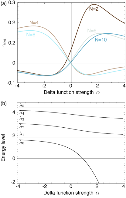
Figure 3: (a) $\gamma_{\mathrm{int}}$ versus $\delta$ function strength $\alpha$ for varying electron number $N$ in the symmetric $\delta$ function potential. Each time $N$ is increased by 2, the sign of $\alpha$ for which the maximum or minimum occurs changes sign. (b) The energy level structure of the symmetric $\delta$ function potential as a function of $\delta$ function strength $\alpha$.

The symmetric triangular well with a $\delta$-function, i.e. eq. (6) with $A_{0}=1$, is known to achieve near-optimal results for $\gamma_{int}$ for $N=1$ despite only containing one free parameter. Due to the simplicity of this potential, it is possible to directly visualize $\gamma_{int}$ as a function of this parameter, the strength of the delta function $\alpha$, for different values of $N$. The results are displayed in fig. 3(a). Immediately apparent is an alternation of the sign of the $\gamma_{int}$ curves as $N$ is increased by 2: for $N=2,6,10...$ the maximum value of $\gamma_{int}$ occurs for positive $\alpha$—corresponding to a $\delta$-function wall in the middle of the well, while for $N=4,8...$ the maximum value of $\gamma_{int}$ occurs for negative $\alpha$. The magnitude of $\alpha$ for which the maxima occur increases only slightly with $N$, however. The behavior of the minimum value of $\gamma_{int}$ is similar, but shifts even less.

Some insight into these results is obtained by examining the effect of the $\delta$-function on the single electron energy level spectrum for the potential, shown in fig. 3(b). Clearly, only the even wavefunctions are affected by the $\delta$-function due to the $\mathcal{P}$-symmetry of the potential. While the placement of $\lambda_{0}$ can be freely adjusted by changing $\alpha$, the higher even energy levels are bounded by their invariant odd neighbors, e.g. $\lambda_{1}<\lambda_{2}<\lambda_{3}$. The freedom of selecting $\lambda_{0}$ relative to $\lambda_{1}$ allows the $N=2$ case to achieve $\gamma$ a high fraction of the Kuzyk maximum, while the restricted higher levels only permit a lower value of $\gamma_{int}$ to be achieved. The reason for the alternation is also apparent. For $N=2$, the Highest Occupied Molecular Orbital (HOMO) in the ground state is $\lambda_{0}$ while the Lowest Unoccupied Molecular Orbital (LUMO) is $\lambda_{1}$; increasing $\alpha$ serves to widen the HOMO-LUMO gap. On the other hand, for $N=4$ the HOMO is $\lambda_{1}$ and the LUMO is $\lambda_{2}$; increasing $\alpha$ for this case serves to narrow the HOMO-LUMO gap. This trend continues with $\alpha$ widening the HOMO-LUMO gap for $N=2,6,10...$ and narrowing the HOMO-LUMO gap for $N=4,8$; the alternating effect of $\alpha$ explains the different signs of $\gamma_{int}$ with $N$.

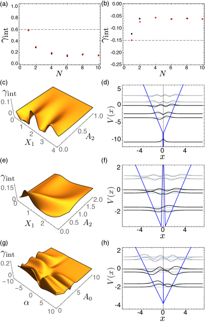
Figure 4: Maximum (a) and minimum (b) $\gamma_{\mathrm{int}}$ achieved for varying increasing numbers of electrons; results for the symmetric linear piecewise potential are shown in red and for the symmetric $\delta$ function potential in black. (c) For $N=8$, the objective function $\gamma_{\mathrm{int}}$ plotted versus the linear piecewise potential shape parameters $A_{2}$ and $X_{1}$ for positive $A_{1}$ and (d) the best potential and wavefunctions obtained. (e) Results for negative $A_{1}$ and (f) the corresponding potential and wavefunctions. (g) Results for the $\delta$ function potential shape parameters $\alpha$ and $A_{2}$ and (h) optimized wavefunctions and potential.

To determine whether these results are universal, we also optimized $\gamma_{int}$ for the asymmetric $\delta$-function potential eq. (6) as well as the linear piecewise potential given by eq. (7). Shown in fig. 4(a) and (b) are the best maximum and minimum $\gamma_{int}$ obtained as a function of $N$. Although there are small differences between results obtained with different potentials, the same trend is clear: that the best $\gamma_{int}$ falls off with increasing $N$ but rapidly reaches a constant value, yielding an apparent feasible range of $-0.05<\gamma_{int}^{max}<0.2$. These apparent bounds are shared by all three potentials.

We plot the objective function results for $N=8$ for several different scenarios: For the linear piecewise potential, the sign of $A_{1}$ must be chosen to be positive or negative prior to optimization. The objective function is shown for $A_{1}=+1$ in fig. 4(c) revealing several local maxima; the corresponding optimized potential, which maximizes $\gamma_{int}$ , and wavefunctions are shown in fig. 4(d). If alternatively, $A_{1}=-1$, a minimum of $\gamma_{int}$ is obtained; the objective function is rather simpler as apparent in fig. 4(e) and the corresponding potential and wavefunctions are shown in fig. 4(f). Note that despite the arbitrariness of the linear potential, the optimized potentials strongly resemble the symmetric $\delta$-function potential, validating its use as ansatz earlier.

Value of $\gamma_{int}$	Potential and Wavefunctions	$A_{0}$	$\alpha$	Hessian eigenvalues	Hessian eigenvectors	$x_{nm}$	$X$	$E$
0.161 (100%)		1.000	-2.963	-0.597, -0.048	$\left(\begin{array}[]{c}-0.999\\ 0.053\end{array}\right)$		0.615	0.765
0.134 (83%)		1.375	2.534	-1.926, -0.039	$\left(\begin{array}[]{c}-0.999\\ -0.004\end{array}\right)$		0.516	0.638
0.127 (79%)		2.043	-3.765	-1.597, -0.039	$\left(\begin{array}[]{c}-0.999\\ 0.024\end{array}\right)$		0.511	0.638
-0.0613 (100%)		1.630	-2.107	6.970, 0.0187	$\left(\begin{array}[]{c}0.999\\ -0.016\end{array}\right)$		0.655	0.500
-0.0609 (99%)		1.000	1.524	13.78, 0.0311	$\left(\begin{array}[]{c}0.999\\ -0.0006\end{array}\right)$		0.654	0.500
-0.0502 (82%)		3.260	2.467	1.162, 0.0123,	$\left(\begin{array}[]{c}0.997\\ -0.069\end{array}\right)$		0.639	0.500

Table 2: Asymmetric $\delta$-function potentials with locally optimal $\gamma_{int}$. Results for each potential are shown as follows, columnwise: the value of $\gamma_{int}$ , and the fraction of the globally optimum value; the potential and wavefunctions; optimized values of the parameters $A_{0}$ and $\delta$; the eigenvalues and eigenvectors of the Hessian matrix of $\gamma_{int}$ with respect to the parameters; a plot of the dipole transition matrix $x_{nm}=\left\langle n\left|x\right|m\right\rangle$ with the HOMO and LUMO indicated by H and L respectively and coloring as described in the text; the energy ratio $E$ and dipole transition moment $X$ for the Kuzyk three-state model.

The asymmetric $\delta$-function potential has a much more complicated landscape for $\gamma_{int}$ as is evident in fig. 4(g). Many local minima and maxima exist. The best three for both positive and negative $\gamma$ are displayed in table 2, together with the parameter values and results of the hessian eigenanalysis. Many of the results above for $\beta$ are also seen for $\gamma$: both attractive and repulsive $\delta$-functions lead to large $\gamma$, in agreement with the phase interruption paradigm. Eigenvalues of the hessian differ by a similar ratio of $\sim 10^{-2}$ and again the eigenvectors are well aligned with the basis vectors of the parameter space. Just as for the first hyperpolarizability with $N=8$ electrons, it appears that $A_{0}$ is the most important parameter.

Intriguingly, the best negative $\gamma_{int}$ obtained does not possess $\mathcal{P}$ symmetry in sharp contrast to the $N=1$ case, although a $\mathcal{P}$-symmetric solution within 1% of this value also exists. It is possible this is due to the freedom of choosing the relative position of the lowest energy level $\lambda_{0}$ relative to $\lambda_{1}$; less freedom exists for the higher single particle energy levels.

Position matrix elements $x_{nm}$ are shown in 2 for each potential. Note that these matrices for $\mathcal{P}$ symmetric potentials have a characteristic checkerboard structure. Elements immediately off the diagonal $\left|n-m\right|=1$ are plotted on a greyscale while non-tridiagonal elements are plotted in red and blue and it is evident, as for $\beta_{int}$, that the matrices are diagonally dominant. For positive $\gamma_{int}$ , the $\mathcal{P}$-symmetric global optimum has large terms on the $|n-m|=3$ off diagonal, which is consistent with a few-state hypothesis; here the HOMO$\to$LUMO+2 and HOMO-1$\to$LUMO+1 terms make the strongest contribution. The transition matrices for the non $\mathcal{P}$-symmetric solutions, however, seem to have little in common with the global optimum, which is perhaps to be expected since the values of $\gamma_{int}$ for these secondary maxima fall some $20\%$ below it.

For negative $\gamma_{int}$, where the two best solutions have nearly identical values, the transition matrix for the $\mathcal{P}$-symmetric optimum resembles the solution for positive $\gamma_{int}$, i.e. HOMO$\to$LUMO+2 and HOMO-1$\to$LUMO+1 are the dominant off-tridiagonal terms. The non $\mathcal{P}$-symmetric solution has an interesting structure: the HOMO$\to$LUMO element is large, while the HOMO$\to$LUMO+1 and HOMO-1$\to$LUMO elements are significantly weaker than the other $\left|n-m\right|=2$ elements. A similar pattern, where off-tridiagonal elements are suppressed around the Fermi surface, is also seen in the third highest optimum that is also non $\mathcal{P}$-symmetric. It is for negative $\gamma_{int}$, therefore, that we find the clearest correspondence with the transition matrix elements of the three-state ansatz.

We now connect these results to the Sum-Over States Formula for $\gamma$, which includes two types of terms: There are both terms involving the ground state and three other states, $m$, $n$, and $l$, energy factors and the matrix element product $x_{0l}x_{0n}x_{lm}x_{nm}$ or $x_{0m}x_{ml}x_{ln}$ which we shall hereafter call “four state” terms. There are also terms involving the ground state and two excited states, $n$, $m$, referred to hence as “three state” terms. A three state term proportional to $(x_{0n}x_{nm})^{2}$ makes a positive contribution to $\gamma$, one proportional to $(x_{0n}x_{0m})^{2}$ will make a negative contribution. This is more easily seen from eq. (73) in Kuzyk et al. (2013), if $m$ is considered the unconstrained summation variable, $n$ and $l$ are (as before) both considered to be different from $m$, and the energy factors are made symmetric in $n$ and $l$. Moreover, only three state terms involving at least one off-tri-diagonal matrix element can contribute. If there are no off-tri-diagonal matrix elements, the matrix elements and energies are constrained to be those for the harmonic oscillator, for which $\gamma=0$. The largest terms in $\gamma$ from four-state terms involves three excited states, three-tridiagonal matrix elements and one matrix element for which $|n-m|=3$. The largest contributions to $\gamma$ from three state terms involves the square of a tri-diagonal matrix element and the square of an $|n-m|=2$ matrix element. These last matrix elements, and so also these terms, are forbidden by $\mathcal{P}$ symmetry.

Now looking at the $x$ matrices, we see that the the $\mathcal{P}$-symmetric potentials have three large contributions, with the signs of these three contributions oscillating with period 2 in the empty state in the highest or lowest singly occupied state. The resultant cancellations may again partly explain the smaller $\gamma_{int}$ achieved for these potentials. The difference between positive and negative $\gamma$ is not the kinds of terms involved (as suggested in Kuzyk (2000b)) but rather in the signs of the off-tridiagonal matrix elements. The three-state terms that are allowed for non $\mathcal{P}$-symmetric potentials are more similar to those considered in Kuzyk (2000b), except that these can have either sign.

To facilitate comparisons with other work, we again computed values of the Kuzyk three-state model parameters $E$ and $X$. For the lower bound, all three extrema favor $E=0.5$ and $X\approx 0.65$. An earlier study by Watkins et al.Watkins and Kuzyk (2012), who optimized $\gamma_{int}$ for different potentials and $N=1$, found for negative $\gamma_{int}$ $X\approx 0.66$ and two clusters of solutions with $E\approx 0.15$ or $E\approx 0.53$. Our results are therefore in excellent agreement. For the upper bound, our results display more variation with $E=0.765$ and $X=0.615$ for the best potential found. Watkins et al. similarly found more variation in positive $\gamma_{int}$, obtaining results around $E\approx 0.57$ with $X\approx 0.5$. As for $\beta$, the discrepancy is explicable because eigenanalysis reveals that effectively only one parameter is truly important, seemingly the slope of the left hand boundary.

III.3 Discussion

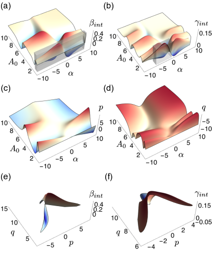
Figure 5: Objective functions (a) $\beta_{int}$ and (b) $\gamma_{int}$ for the asymmetric $\delta$-function potential shown in the natural parameter space $A_{0}$ and $\alpha$; wavefunction parameters at the classical turning points (c) $p=\psi_{l}^{\prime}/\psi_{r}^{\prime}-\psi_{r}^{\prime}/\psi_{l}^{\prime}$ and (d) $q=-\Delta x^{2}\left|\psi^{\prime}_{l}\psi^{\prime}_{r}\right|^{2/3}$ plotted with respect to $A_{0}$ and $\alpha$. A selected region of the objective function, enclosed in the grey volume in (a) and (b), is show replotted with respect to $p$ and $q$ in (e) and (f) respectively.

The above subsections have presented optimized potentials for $\beta_{int}$ and $\gamma_{int}$ with increasing $N$, expressed in a parameter space that a posteriori is found to coincide with what is important to the hyperpolarizabilities. As discussed, this is a significant development over previous work, where the parameter space was larger the optimized potentials gave a less clear sense of which features are important. Nonetheless, the parameters $A_{0}$ and $\alpha$ are an artifact of the parameterization chosen, and it is therefore desirable to identify quantities that are invariant under reparametrization and rescaling of the form in eq. (5). This is particularly important because, if we generalize to the space of arbitrary potentials, there are many other solutions with identical values of the hyperpolarizability. For the $N=1$ case, we know that the hyperpolarizabilities can be completely reconstructed from the ground state wavefunctionWiggers and Petschek (2007). Extending this to the $N>1$ case, it is easy to see that the hyperpolarizablities can be constructed for this problem as appropriate integrals of the occupied single particle wavefunctions alone. As the largest term is expected to the HOMO, the important parameters ought to be expressible in terms of parameters crucial to the HOMO.

Moreover, there is a need to connect the dipole-free sum-over-states view, which prescribes certain values of the dipole transition matrix elements, and the potential view that we pursued above. We therefore performed an approximate analysis of the problem, inserting WKB ansatz wavefunctions into expressions for $E_{nm}$ and $x_{nm}$ to determine what details of these wavefunctions most significantly affect these parameters. The full calculations presented in the Appendix below support this argument and suggest that the three parameters introduced in the next paragraph are the crucial ones..

On the basis of approximate analytic arguments made in the appendix, and a numerical experiment that follows, we believe that there are three length scales that are important to the hyperpolarizabilities around the maximum. One is $\Delta x$, the separation between the turning points of the HOMO. The other two are length scales $L_{k}$ for $k$ and an element of $\{r,l\}$ that characterizes the rate at which the wavefunction varies near the right and left turning points of the HOMO. A variety of nearly equivalent forms can be given for these lengths and dimensionless ratios containing them, including $L=(V^{\prime})^{-1/3}$, and more global formulae related the derivatives of the wavefunction at the turning points or to the normalization of the HOMO. From these three lengths, it is possible to construct two dimensionless parameters that are arguably important to the hyperpolarizability, for example,

$$p = \psi_{l}^{\prime}/\psi_{r}^{\prime}-\psi_{r}^{\prime}/\psi_{l}^{\prime}$$

$$q = -\Delta x^{2}\left|\psi^{\prime}_{l}\psi^{\prime}_{r}\right|^{2/3}$$ (19)

are invariant under reparameterization and rescaling. Here $\Delta x$ is the distance between the turning points, $\psi_{l}^{\prime}$ and $\psi_{r}^{\prime}$ are the slopes of the wavefunctions where the subscripts $l$ and $r$ refer to the left and right turning point respectively. As some of the definitions of $L$ are zero when $V^{\prime}$ is infinite at the turning points, and it is still possible for the hyperpolarizabilities to approach the maximum in this case, appropriate dimensionless combinations should not be infinite in this limit. As $\beta_{int}$ requires asymmetry in the potential, it is expected that a parameter odd under $\mathcal{P}$ symmetry, such as $p$, mostly controls $\beta$ while one even under $\mathcal{P}$ symmetry, such as $q$, mostly controls $\gamma_{int}$.

In fig. 5 we show the objective functions (a) $\beta_{int}$ and (b) $\gamma_{int}$ plotted in the parameter space of the asymmetric $\delta$-function potential, i.e. $A_{0}$ and $\alpha$. In the same parameter space, we show in 5(c) and (d) the values of the wavefunction parameters $p$ and $q$ from eq. (19). From these plots, we see that much of the structure in the objective functions $\beta_{int}$ and $\gamma_{int}$ is attributable to these new parameters: notice that the position of the ridges in 5(c) corresponds to the ridges in 5(a), while those in 5(d) corresponds, more roughly, those in 5(b). In figs. 5(e) and (f), the portion of the objective function in figs. 5(a) and (b) that is enclosed within the grey cuboid is reprojected into the new ($p$, $q$) parameter space. Plots of the objective functions—not shown here—in $(p,q)$ space for the full range of $(A_{0},\alpha)$ from fig. 5(a) and (b) closely resemble the structure observed in this reduced reduced region.

From these results, we conclude that $\beta_{int}$ is largely determined by $p$ while $\gamma_{int}$ is largely determined by $q$, and the remaining parameter in each case must be tuned less precisely to achieve the optimum. It is also now clear that the asymmetric $\delta$-function performs so well due to a fortuitous correspondence: the $A_{0}$ parameter directly controls the ratio of the slope of the potentials at the turning points, which is readily related to the slope of the wavefunctions at the classical turning points, i.e $A_{0}$ and $p$ are simply related.

	Optimum value	$p$	$q$
$\beta_{int}$	$0.403$	$1.69$	$-8.99$
	$-0.372$	$-1.28$	$-7.66$
	$0.370$	$2.11$	$-9.26$
$\gamma_{int}$$>0$	$0.161$	$0$	$-9.30$
	$0.134$	$-1.85$	$-6.40$
	$0.126$	$-1.88$	$-6.95$
$\gamma_{int}<0$	$-0.0613$	$0.456$	$-10.54$
	$-0.0610$	$-1.02\times 10^{-5}$	$-9.30$
	$-0.0503$	$1.214$	$-10.54$

Table 3: Values of dimensionless parameters $p$ and $q$ constructed from the HOMO wavefunction for each of the optimized $N=8$ solutions displayed in tables 1 and 2

		$N$
		$2$	$4$	$6$	$8$	$10$
$\beta_{int}$	$p$	$-4.17$	$1.94$	$-2.52$	$1.69$	$-1.96$
	$q$	$-1.37$	$-4.00$	$-7.11$	$-8.99$	$-12.6$
$\gamma_{int}$$>0$	$p$		$5.15\times 10^{-3}$	$2.08$	$0$	$1.92$
	$q$		$-3.64$	$-4.97$	$-9.30$	$-9.62$
$\gamma_{int}<0$	$p$		$0$	$0$	$0.456$	$0$
	$q$		$-3.65$	$-7.35$	$-10.5$	$-13.2$

Table 4: Dimensionless parameters $p$ and $q$ calculated from the best solution found as a function of $N$.

We display in table 3 the values of $p$ and $q$ calculated for each of the optima of $\beta_{int}$ and $\gamma_{int}$ shown in table 1 and 2. For each of the optimization problems, i.e. $\left|\beta_{int}\right|$, $\gamma_{int}>0$ and $\gamma_{int}<0$ the values of at least one of these parameters are internally quite consistent with each other. This is particularly so for the negative $\gamma_{int}$ results where the secondary optima are close to the global optimum. Values of $p$ and $q$ for the global optimum as a function of $N$ are shown in table 4. These reveal several trends: First $\text{sgn}(\beta_{int})=\text{sgn}(p)(-1)^{n_{nh}}$ where $n_{nh}$ is the number of nodes in the HOMO. Otherwise, it is expected that $\mathcal{P}$ symmetry just changes the sign of $\beta_{int}$ and $p$. Also, a sign alternation occurs in $p$ for $\beta_{int}$; $q$ seems to increase with $N$ for $\gamma_{int}$, while $p$ is found alternately $0$ or some small value. The a posteriori consistency of these parameters supports the argument above that these are the “real” parameters of the optimization problem.

IV Conclusion

We have optimized the intrinsic hyperpolarizabilities $\beta_{int}$ and $\gamma_{int}$ for non-interacting multi-electron systems with respect to the shape of several classes of potential: a piecewise linear potential, and an asymmetric triangular well with a $\delta$-function. The best values obtained for $\beta_{int}$ and $\gamma_{int}$ drop from the $N=1$ case and approach an apparent feasible range of $\left|\beta_{int}\right|<0.4$ and $-0.05<\gamma_{int}^{max}<0.2$ for $N$ larger than around eight electrons. The asymmetric $\delta$-function potential achieves these bounds and, due to the small number of parameters, and a posteriori verification that the parameters are indeed relevant, provides a design prototype for synthesis of new chromophores. For $\beta_{int}$, a molecule should have asymmetric walls and possess an attractive or repulsive feature in the middle—a main chain functional group or side-chain—that promotes a rapid change in the phase of the wavefunction. The asymmetry of the boundary and the strength of the attraction or repulsion should then be tuned to achieve high $\beta_{int}$. For $\gamma_{int}$, the molecule should be essentially $\mathcal{P}$-symmetric with a central attractive or repulsive feature that should similarly be tuned.

By approximate analysis, we also determined that the ad hoc parameters of our potential can be re-expressed in terms of the dimensionless, scale invariant parameters derived from the shape of the HOMO wavefunction at the classical turning points. These new parameters are important both because they explain the success of our original parametrization and because they provide a new wavefunction-centered approach to screen potential chromophores for large hyperpolarizabilities.

The results also provide important information on how well the many theoretical studies of single electron systems might describe real molecules that posses multiple electrons. While the apparent bounds quoted above are more restrictive than the $N=1$ case, it seems, encouragingly, that the overall design paradigms described above apply equally well to both cases. Information from other studies on target values of the $E$ and $X$ parameters of the three state model for $N=1$ also seems to remain valid with increasing $N$. The insights of Atherton et al. (2012); Burke et al. (2013) that only a very small number of parameters are required remain valid, and happily, this appears to be increasingly so with large $N$. Because of this and because the objective function for multiple electrons acquires many more local extrema, it should in principle be easier to tune multi-electron systems.

Appendix A Approximate Analysis

In this appendix we use approximate techniques to argue that the dimensionless parameters identified in the main text constructed from the separation between the turning points of the HOMO and the slopes of the potential at these turning points ought to mostly explain the hyperpolarizability. The simple, zeroth order argument is given in the next two paragraphs. A more detailed but still very approximate calculation follows.

For all potentials with large hyperpolarizabilities, the transition matrix elements between the frontier wavefunctions—those that are close to the Fermi level—must be large. When these matrix elements are large, there are very strong constraints on the energy differences between the various states, and hence we can regard these parameters are fixed by the matrix elements and we need only calculate the transition matrix elements to predict the hyperpolarizabilities.

In order to calculate these transition matrix elements approximately, we note that wavefunctions fall rapidly in the classically forbidden region and oscillate in the classically allowed region. Thus most of the transition matrix integral between two states necessarily comes from the region between or very close to the turning point of the lower energy state. Moreover, far from the turning points, each wavefunction becomes relatively small, in effect because the particles are (classically) moving relatively quickly. Thus most of the contribution to these integrals comes from the region close to the turning point of the lower energy wavefunction. From this it is clear that the distance between the turning points of the HOMO is an important parameter.

The wavefunction near a turning point is constrained by the slope of the potential at the turning point. Moreover, the ratio of the amplitudes of the wavefunction at the two turning points is limited by general principles, described below. While the wavefunction of the higher energy state near the turning points of the lower energy states is more free to vary, provided the potential is not too far from linear, they are still largely constrained by the slope of the potential. Thus the slopes of the potential at the turning points of the HOMO also seems to be a very important parameter. From these parameters, it is possible to construct two dimensionless parameters, and it is known from numerical experiments that only two parameters seem to be important to maximizing hyperpolarizabilities for model potentials.

We now provide a more detailed, but nonetheless approximate, analysis. We begin with the sum-over-states formulae for the hyperpolarizabilities. For instance, the off-resonant expression for the second hyperpolarizability is,

$$\gamma_{xxxx}=2e^{4}\left(2\sum_{lmn}^{\infty}{}^{{}^{\prime}}\frac{x_{0l}\bar{x}_{lm}\bar{x}_{mn}x_{n0}}{E_{l0}E_{m0}E_{n0}}-\sum_{mn}^{\infty}{}^{{}^{\prime}}x_{0m}^{2}x_{0n}^{2}\left\{\frac{1}{E_{m0}^{2}E_{n0}}+\frac{1}{E_{n0}^{2}E_{m0}}\right\}\right),$$ (20)

which contains three kinds of quantity: the energy level differences $E_{nm}=E_{n}-E_{m}$, matrix elements $x_{nm}=\left\langle n\left|x\right|m\right\rangle$ and barred quantities $\bar{x}_{nm}$ that contain dipole terms,

$$\bar{x}_{nm}=\begin{cases}\Delta x_{n0}=x_{nn}-x_{00}&,\ n=m\\ x_{nm}&,\ n\neq m\end{cases}.$$ (21)

As is well known, the dipole terms can be eliminated from these expressions using the sum rulesPérez-Moreno et al. (2008); Kuzyk (2005), leaving only the transition elements $x_{nm}$ and energy level differences $E_{nm}$. Numerous previous studies, as well as the results above, have shown that only a few states—in fact 2-3—near the Fermi energy contribute significantly to the hyperpolarizabilities. Hence, the question of what is important to the hyperpolarizability maybe be addressed by understanding how the potential and wavefunctions affect these quantities. In the remainder of the appendix, we will answer this question by constructing WKB ansatz wavefunctions, inserting them into expressions for these quantities and examining the form of the results.

In order to proceed, we make some simplifying assumptions. First, we assume that the true optimum potential is sufficiently smooth that the WKB approximation yields good approximations, at least near the turning points, to the relevant wavefunctions, i.e. those near the Fermi surface. This is justified by previous studiesWiggers and Petschek (2007) that have shown the addition of small rapidly varying perturbations to the potential doesn’t affect the hyperpolarizabilities. The ansatz potentials studied in this work, with delta functions and changes in slope at isolated points, all satisfy this criterion.

Second, we shall assume that for wavefunctions near the Fermi energy there are only two classical turning points, except possibly for isolated delta functions in the potential that may violate this rule. We justify this because the presence of multiple turning points would result, at least approximately, in roughly independent particles in the separate classically allowed regions. This would lead to hyperpolarizabilities that grow $\propto N$ rather than $\propto N^{\frac{3}{2}}$ (for $\beta$) or $\propto N^{2}$ (for $\gamma$) as the Kuzyk bounds imply. The turning points shall be denoted $x_{n}^{l}$ and $x_{n}^{r}$, corresponding to the left and right turning point respectively, and are found by solving $V(x_{n}^{l})=E_{n}$ . In this expression, and hereafter, $l$ indexes the left or right turning point.

Within the above assumptions it is possible to write an ansatz wavefunction for the $n$th state that is valid except for the region near the classical turning points,

$$\psi_{n}(x)=\begin{cases}A_{n}(x)\cos\left[\phi_{n}(x)-\Delta\phi_{n}(x)\right],&E>V\\ A_{n}(x)\exp\left[-\gamma_{n}^{l}(x)\right],&E<V\end{cases}$$ (22)

where $E>V$ and $E<V$ refer to the classically allowed and forbidden regions respectively. The functions $\gamma_{n}^{l}$ are defined by,

$$\gamma_{n}^{l}(x)=\left|\int_{x_{n}^{l}}^{x}\left(V(x^{\prime})-E_{n}\right)^{\frac{1}{2}}dx^{\prime}\right|,$$ (23)

and the function $\phi_{n}(x)$ is given by,

$$\phi_{n}(x)=\frac{\pi}{4}+\int_{x_{n}^{<}}^{x}\left(E_{n}-V(x^{\prime})\right)^{\frac{1}{2}}dx^{\prime}.$$ (24)

The remaining functions $A_{n}(x)$ and $\Delta\phi_{n}(x)$ are smooth and slowly varying, except where the potential has delta functions or sharp changes; nonetheless they are necessarily smoother than the potential. For the smooth potentials considered here, $\Delta\phi(x)$ is of order $\pi$ or smaller. $A(x)$ is relatively close to the semiclassical result $A(x)\approx a(x)v(x)^{\frac{1}{2}}$ where $v(x)$ is the classical velocity and $a(x)$ changes only by amounts that are asymptotically small where the WKB approximation is valid, except very close to the turning points. The dependence of $a(x)$ can easily be made more precise by using the uniform asymptotic WKB approximation to the wavefunctionBender and Orszag (1999) though this does little to illuminate the discussion. Moreover, even if WKB is invalid somewhere between the turning points, the magnitude, $|a(x)|$ is, roughly speaking, the rate at which the electron "turns" at the turning point and so is expected to be the same at both turning points. In WKB there is no reflection in classically allowed regions and hence it is obvious that $|a(x)|$ cannot change. More generally, however, any structure between the turning points must have equal magnitude for the transmission and reflection from each side. This implies that $|a(x)|$ must have the same values at both turning points. Moreover, $a(x)$ can be chosen to be real near both turning points, and the ratio of $a$ near the two turning points alternates sign as we increase the energy of the wavefunctions.

The approximate energies are found, as usual, by solving

$$n+\frac{1}{2}=\phi(x_{n}^{>})=\int_{x_{n^{l}}}^{x_{n}^{r}}\left(E_{n}-V(x^{\prime})\right)^{\frac{1}{2}}dx^{\prime}.$$ (25)

Combining copies of the WKB equation (25) for two different states $n$ and $m$, we obtain,

$$n-m=\int_{x_{n^{l}}}^{x_{n}^{r}}\left(E_{n}-V(x^{\prime})\right)^{\frac{1}{2}}dx^{\prime}-\int_{x_{m}^{l}}^{x_{m}^{r}}\left(E_{m}-V(x^{\prime})\right)^{\frac{1}{2}}dx^{\prime}.$$ (26)

These integrals may be combined by making a linear change of variable $x^{\prime}\to x_{p}^{l}+y\Delta x_{p}$ where $y\in[0,1]$ and $\Delta x_{p}=x_{p}^{r}-x_{p}^{l}$.

$$n-m=\int_{0}^{1}dy\left[\Delta x_{p}\left[E_{n}-V\left(x_{n}^{l}+y\Delta x_{p}\right)\right]^{\frac{1}{2}}-\Delta x_{p}\left[E_{m}-V\left(x_{m}^{l}+y\right)\right]^{\frac{1}{2}}\right].$$ (27)

The square roots in the integrand can be combined by completing the square,

$$n-m=\int_{0}^{1}dy\frac{\Delta x_{n}^{2}\left[E_{n}-V(\Delta x_{n}y+x_{n}^{l})\right]-\Delta x_{t,m}^{2}\left[E_{m}-V(\Delta x_{m}y+x_{m}^{l}\right]}{\Delta x_{n}\left[E_{n}-V(\Delta x_{n}y+x_{n}^{l})\right]+\Delta x_{t,m}\left[E_{m}-V(\Delta x_{m}y+x_{m}^{l})\right]}.$$ (28)

The form of the integrand in (28) is instructive: near the turning points, i.e. as $y\to 0$ and $y\to 1$, the numerator goes to zero linearly in $y$ while the denominator goes to zero as a square root; the integrand therefore vanishes like $y^{1/2}$ near the turning points. Hence, the majority contribution to this integral comes from the spatial region far from the classical turning points, particularly if the two energies are similar and the potential near the turning points is slowly varying. Moreover, this integral tends to smooth out small, high frequency variations in the potential; it follows that if $\left|n-m\right|$ is small, then $E_{n}-E_{m}$ is largely determined by the form of the potential far from the turning points.

We now turn to the dipole matrix elements $x_{nm}$, which can be computed using the position formula,

$$x_{nm}=\int_{-\infty}^{\infty}dxx\psi_{n}\psi_{m}.$$ (29)

We shall restrict our analysis to small values of $\left|n-m\right|$, because only these states contribute significantly to the hyperpolarizability. Moreover, approximate analysis of these integrals is complicated for large $\left|n-m\right|$ because, while small, they are strongly dependent on the detailed analytic behavior of the potential and wavefunctions.

Substituting the ansatz wavefunction (22) into the position formula (29),

$$x_{nm}\approx\int_{x_{m}^{<}}^{x_{m}^{>}}dx\frac{1}{2}A_{n}A_{m}\left[x-\frac{1}{2}(x_{t,m}^{r}+x_{t,n}^{l})\right]\cos(\phi_{n}-\phi_{m}+\Delta\phi_{m}-\Delta\phi_{m}),$$ (30)

. This integral is then the integral of a function that has $n-m-1$ nodes, roughly evenly spaced through the interval, and has a somewhat (algebraically) larger magnitude near the turning points. From this formula, it is apparent that the transition matrix elements depend primarily on the nature of the wavefunctions near the classical turning points, i.e. separation between the two turning points and as well as the shape of the wavefunctions in their vicinity. As the shape of the wavefunctions are most dependent on the slopes of the potential at the turning points and there must be a connection between the energy differences and the transition matrix elements, this strongly argues that the separation between the turning points of the HOMO and the slopes of the potential at these turning points should be among the most important heuristic parameters that determine the hyperpolarizabilities.

References

- Kuzyk et al. (2013) M. G. Kuzyk, J. Perez-Moreno, and S. Shafei, Physics Reports 529, 297 (2013).
- Mossman and Kuzyk (2013) S. M. Mossman and M. G. Kuzyk, “Optimizing hyperpolarizability through the configuration space of energy spectrum and transition strength spanned by power law potentials,” (2013).
- Watkins and Kuzyk (2012) D. S. Watkins and M. G. Kuzyk, J. Opt. Soc. Am. B 29, 1661 (2012).
- Atherton et al. (2012) T. Atherton, J. Lesnefsky, G. Wiggers, and R. Petschek, Journal of the Optical Society of America B: Optical Physics 29, 513 (2012).
- Burke et al. (2013) C. J. Burke, T. Atherton, J. Lesnefsky, and R. Petschek, JOSA B 30, 1438 (2013).
- Lytel et al. (2013) R. Lytel, S. Shafei, J. H. Smith, and M. G. Kuzyk, Phys. Rev. A 87, 043824 (2013).
- Lytel and Kuzyk (2013) R. Lytel and M. G. Kuzyk, Journal of Nonlinear Optical Physics & Materials 22, 1350041 (2013).
- Lytel et al. (2014) R. Lytel, S. Shafei, and M. G. Kuzyk, Journal of Nonlinear Optical Physics & Materials 23, 1450025 (2014).
- Lytel et al. (2015) R. Lytel, S. M. Mossman, and M. G. Kuzyk, Journal of Nonlinear Optical Physics and Materials 24, 1550018 (2015).
- Watkins and Kuzyk (2011) D. S. Watkins and M. G. Kuzyk, The Journal of chemical physics 134, 094109 (2011).
- Kuzyk (2000a) M. G. Kuzyk, Physical review letters 85, 1218 (2000a).
- Tripathy et al. (2004) K. Tripathy, J. P. Moreno, M. G. Kuzyk, B. J. Coe, K. Clays, and A. M. Kelley, The Journal of Chemical Physics 121, 7932 (2004).
- Zhou et al. (2007) J. Zhou, U. B. Szafruga, D. S. Watkins, and M. G. Kuzyk, Phys. Rev. A 76, 053831 (2007).
- Kuzyk (2000b) M. G. Kuzyk, Opt. Lett. 25, 1183 (2000b).
- Wiggers and Petschek (2007) G. A. Wiggers and R. G. Petschek, Opt. Lett. 32, 942 (2007).
- Pérez-Moreno et al. (2008) J. Pérez-Moreno, K. Clays, and M. G. Kuzyk, The Journal of Chemical Physics 128, 084109 (2008).
- Kuzyk (2005) M. G. Kuzyk, Phys. Rev. A 72, 053819 (2005).
- Bender and Orszag (1999) C. Bender and S. Orszag, Advanced Mathematical Methods for Scientists and Engineers I: Asymptotic Methods and Perturbation Theory, Advanced Mathematical Methods for Scientists and Engineers (Springer, 1999).