Robust Influence Maximization

Uncertainty about models and data is ubiquitous in the computational social sciences, and it creates a need for robust social network algorithms, which can simultaneously provide guarantees across a spectrum of models and parameter settings. We begin an investigation into this broad domain by studying robust algorithms for the Influence Maximization problem, in which the goal is to identify a set of $k$ nodes in a social network whose joint influence on the network is maximized.

We define a Robust Influence Maximization framework wherein an algorithm is presented with a set of influence functions, typically derived from different influence models or different parameter settings for the same model. The different parameter settings could be derived from observed cascades on different topics, under different conditions, or at different times. The algorithm’s goal is to identify a set of $k$ nodes who are simultaneously influential for all influence functions, compared to the (function-specific) optimum solutions.

We show strong approximation hardness results for this problem unless the algorithm gets to select at least a logarithmic factor more seeds than the optimum solution. However, when enough extra seeds may be selected, we show that techniques of Krause et al. can be used to approximate the optimum robust influence to within a factor of $1-1/e$. We evaluate this bicriteria approximation algorithm against natural heuristics on several real-world data sets. Our experiments indicate that the worst-case hardness does not necessarily translate into bad performance on real-world data sets; all algorithms perform fairly well.

1 Introduction

Computational social science is the study of social and economic phenomena based on electronic data, algorithmic approaches and computational models. It has emerged as an important application of data mining and learning, while also invigorating research in the social sciences. Computational social science is frequently envisioned as a foundation for a discipline one could term “computational social engineering,” wherein algorithmic approaches are used to change or mitigate individuals’ behavior.

Among the many concrete problems that have been studied in this context, perhaps the most popular is Influence Maximization. It is based on the observation that behavioral change in individuals is frequently effected by influence from their social contacts. Thus, by identifying a small set of “seed nodes,” one may influence a large fraction of the social network. The desired behavior may be of social value, such as refraining from smoking or drug use, using superior crops, or following hygienic practices. Alternatively, the behavior may provide financial value, as in the case of viral marketing, where a company wants to rely on word-of-mouth recommendations to increase the sale of its products.

1.1 Prevalence of Uncertainty and Noise

Contrary to the “hard” sciences, the study of social networks — whether using traditional or computational approaches — suffers from massive amounts of noise inherent in the data and models. The reasons range from the fundamental to the practical:

• At a fundamental level, it is not even clear what a “social tie” is. Different individuals or researchers operationalize the intuition behind “friendship”, “acquaintance”, “regular” advice seeking, etc. in different ways (see, e.g., [4]). Based on different definitions, the same real-world individuals and behavior may give rise to different mathematical models of the same “social network.”

• Mathematical models of processes on social networks (such as opinion adoption or tie formation) are at best approximations of reality, and frequently mere guesses or mathematically convenient inventions. Furthermore, the models are rarely validated against real-world data, in large part due to some of the following concerns.

• Human behavior is typically influenced by many environmental variables, many of them hard or impossible to measure. Even with the rapid growth of available social data, it is unlikely that data sets will become sufficiently rich to disentangle the dependence of human behavior on the myriad variables that may shape it.

• Observational data on social behavior is virtually always incomplete. For example, even if API restrictions and privacy were not concerns (which they definitely are at this time) and a “complete” data set of Twitter and Facebook and e-mail communication were collected, it would still lack in-person and phone interactions.

• Inferring model parameters relies on a choice of model and hyperparameters, many of which are difficult to make. Furthermore, while for many models, parameter inference is computationally efficient, this is not universally the case.

Since none of these issues are likely to be resolved anytime soon, both the models for social network processes and their inferred parameters must be treated with caution. This is true both when one wants to draw scientific insight for its own sake, and when one wants to use the inferred models to make computational social engineering decisions. Indeed, the correctness guarantees for algorithms are predicated on the assumption of correctness of the model and the inferred parameters. When this assumption fails — which is inevitable — the utility of the algorithms’ output is compromised. Thus, to make good on the claims of real-world relevance of computational social science, it is imperative that the research community focus on robustness as a primary design goal.

1.2 Modeling Uncertainty in Influence Maximization

We take an early step in this bigger agenda, studying robustness in the context of the well-known Influence Maximization problem. (Detailed definitions are given in Section 3.) In Influence Maximization, the algorithm selects a set $S_{0}$ of seed nodes, of pre-specified size $k$. The seed nodes are initially exposed to a product or idea; we say that they are active. Based on a probabilistic model of influence propagation, they cause some of their neighbors to become active, who then cause some of their neighbors to become active, etc.; this process leads to a (random) final set of active nodes. The goal is to maximize the size of this set; we denote this quantity by $\sigma(S_{0})$.

The concerns discussed above combine to lead to significant uncertainty about the function $\sigma$: different models give rise to very different functional forms of $\sigma$, and missing observations or approximations in inference lead to uncertainty about the models’ parameters.

To model this uncertainty, we assume that the algorithm is presented with a set $\Sigma$ of influence functions, and assured that one of these functions actually describes the influence process, but not told which one. The set $\Sigma$ could be finite or infinite. A finite $\Sigma$ could result from a finite set of different information diffusion models that are being considered, or from of a finite number of different contexts under which the individuals were observed (e.g., word-of-mouth cascades for different topics or products), or from a finite number of different inference algorithms or algorithm settings being used to infer the model parameters from observations. An infinite (even continuous) $\Sigma$ arises if each model parameter is only known to lie within some given interval; this model of adversarial noise, which we call the Perturbation Interval model, was recently proposed in [24].

Since the algorithm does not know $\hat{\sigma}$, in the Robust Influence Maximization problem, it must “simultaneously optimize” for all objective functions in $\Sigma$, in the sense of maximizing $\rho(S_{0})=\min_{\hat{\sigma}\in\Sigma}\frac{\hat{\sigma}(S_{0})}{\hat{\sigma}(\hat{S})}$, where $\hat{S}\in\operatorname{argmax}_{S}\hat{\sigma}(S)$ is an optimal solution knowing which function $\hat{\sigma}$ is to be optimized. In other words, the selected set should simultaneously get as close as possible to the optimal solutions for all possible objective functions.

1.3 Our Approach and Results

Our work is guided by the following overarching questions:

1. How well can the objective $\rho$ be optimized in principle?

2. How well do simple heuristics perform in theory?

3. How well do simple heuristics perform in practice?

4. How do robustly and non-robustly optimized solutions differ qualitatively?

We address these questions as follows. First, we show (in Section 4) that unless the algorithm gets to exceed the number of seeds $k$ by at least a factor $\ln|\Sigma|$, approximating the objective $\rho$ to within a factor $O(n^{1-\epsilon})$ is NP-hard for all $\epsilon>0$.

However, when the algorithm does get to exceed the seed set target $k$ by a factor of $\ln|\Sigma|$ (times a constant), much better bicriteria approximation guarantees can be obtained. Specifically, we show that a modification of an algorithm of Krause et al. [27] uses $O(k\ln|\Sigma|)$ seeds and finds a seed set whose influence is within a factor $(1-1/e)$ of optimal.

We also investigate two straightforward heuristics:

1. Run a greedy algorithm to optimize $\rho$ directly, picking one node at a time.

2. For each objective function $\sigma\in\Sigma$, find a set $S_{\sigma}$ (approximately) maximizing $\sigma(S_{\sigma})$. Evaluate each of these sets under $\rho(S_{\sigma})$, and keep the best one.

We first exhibit instances on which both of the heuristics perform very poorly. Next (in Section 5), we focus on more realistic instances , exemplifying the types of scenarios under which robust optimization becomes necessary. In the first set of experiments, we infer influence networks on a fixed node set from Twitter cascades on different topics. Individuals’ influence can vary significantly based on the topic, and for a previously unseen topic, it is not clear which inferred influence network to use. In additional sets of experiments, we derive data sets from the same MemeTracker data [29], but use different time slices, different inference algorithms and parametrizations, and different samples from confidence intervals.

The main outcome of the experiments is that while the algorithm with robustness as a design goal typically (though not even always) outperforms the heuristics, the margin is often quite small. Hence, heuristics may be viable in practice, when the influence functions are reasonably similar. A visual inspection of the nodes chosen by different algorithms reveals how the robust algorithm “hedges its bets” across models, while the non-robust heuristic tends to cluster selected nodes in one part of the network.

1.4 Stochastic vs. Adversarial Models

Given its prominent role in our model, the decision to treat the choice of $\hat{\sigma}$ as adversarial rather than stochastic deserves some discussion.

First, adversarial guarantees are stronger than stochastic guarantees, and will lead to more robust solutions in practice. Perhaps more importantly, inferring a Bayesian prior over influence functions in $\Sigma$ will run into exactly the type of problem we are trying to address in the first place: data are sparse and noisy, and if we infer an incorrect prior, it may lead to very suboptimal results. Doing so would next require us to establish robustness over the values of the hyperparameters of the Bayesian prior over functions.

Specifically for the Perturbation Interval model, one may be tempted to treat the parameters as drawn according to some distribution over their possible range. This approach was essentially taken in [2, 21]. Adiga et al. [2] assume that for each edge $e$ independently, its presence/absence was misobserved with probability $\epsilon$, whereas Goyal et al. [21] assume that for each edge, the actual parameter is perturbed with independent noise drawn uniformly from a known interval. In both cases, under the Independent Cascade model (for example), the edge activation probability can be replaced with the expected edge activation probability under the random noise model, which will provably lead to the exact same influence function $\sigma$. Thus, independent noise for edge parameters, drawn from a known distribution, does not augment the model in the sense of capturing robustness. In particular, it does not capture uncertainty in a meaningful way.

To model the type of issues one would expect to arise in real-world settings, at the very least, noise must be correlated between edges. For instance, certain subpopulations may be inherently harder to observe or have sparser data to learn from. However, correlated random noise would result in a more complex description of the noise model, and thus make it harder to actually learn and verify the noise model. In particular, as discussed above, this would apply given that the noise model itself must be learned from noisy data.

2 Related Work

Based on the early work of Domingos and Richardson [13, 38], Kempe et al. [25] formally defined the problem of finding a set of influential individuals as a discrete optimization problem, proposing a greedy algorithm with a $1-1/e$ approximation guarantee for the Independent Cascade [16, 17] and Linear Threshold [23] models. A long sequence of subsequent work focused on more efficient algorithms for Influence Maximization (both with and without approximation guarantees) and on broadening the class of models for which guarantees can be obtained [3, 7, 9, 25, 26, 33, 40, 41]. See the recent book by Chen et al. [5] and the survey in [25] for more detailed overviews.

As a precursor to maximizing influence, one needs to infer the influence function $\sigma$ from observed data. The most common approach is to estimate the parameters of a particular diffusion model [1, 11, 18, 19, 35, 37, 39]. Theoretical bounds on the required sample complexity for many diffusion models have been established, including [1, 35, 37] for the Discrete-Time Independent Cascade (DIC) model, [11] for the Continuous-Time Independent Cascade (CIC) model, and [35] for the Linear Threshold model. However, it remains difficult to decide which diffusion models fit the observation best. Moreover, the diffusion models only serve as a rough approximation to the real-world diffusion process. In order to sidestep the issue of diffusion models, Du et al. [14] recently proposed to directly learn the influence function $\sigma$ from the observations, without assuming any particular diffusion model. They only assume that the influence function is a weighted average of coverage functions. While their approach provides polynomial sample complexity, they require a strong technical condition on finding an accurate approximation to the reachability distribution. Hence, their work remains orthogonal to the issue of Robust Influence Maximization.

Several recent papers take first steps toward Influence Maximization under uncertainty. Goyal, Bonchi and Lakshmanan [21] and Adiga et al. [2] study random (rather than adversarial) noise models, in which either the edge activation probabilities $p_{u,v}$ are perturbed with random noise [21], or the presence/absence of edges is flipped with a known probability [2]. Neither of the models truly extends the underlying diffusion models, as the uncertainty can simply be absorbed into the probabilistic activation process.

Another approach to dealing with uncertainty is to carry out multiple influence campaigns, and to use the observations to obtain better estimates of the model parameters. Chen et al. [8] model the problem as a combinatorial multi-armed bandit problem and use the UCB1 algorithm with regret bounds. Lei et al. [28] instead incorporate beta distribution priors over the activation probabilities into the DIC model. They propose several strategies to update the posterior distributions and give heuristics for seed selection in each trial so as to balance exploration and exploitation. Our approach is complementary: even in an exploration-based setting, there will always be residual uncertainty, in particular when exploration budgets are limited.

The adversarial Perturbation Interval model was recently proposed in work of the authors [24]. The focus in that work was not on robust optimization, but on algorithms for detecting whether an instance was likely to suffer from high instability of the optimal solution. Optimization for multiple scenarios was also recently used in work by Chen et al. on tracking influential nodes as the structure of the graph evolves over time [10]. However, the model explicitly allowed updating the seed set over time, while our goal is simultaneous optimization.

Simultaneously to the present work, Chen et al. [6] and Lowalekar et al. [32] have been studying the Robust Influence Maximization problem under the Perturbation Interval model [24]. Their exact formulations are somewhat different. The main result of Chen et al. [6] is an analysis of the heuristic of choosing the best solution among three candidates: make each edge’s parameter as small as possible, as large as possible, or equal to the middle of its interval. They prove solution-dependent approximation guarantees for this heuristic.

The objective of Lowalekar et al. [32] is to minimize the maximum regret instead of maximizing the minimum ratio. They propose a heuristic based on constraint generation ideas to solve the robust influence maximization problem. The heuristic does not come with approximation guarantees; instead, [32] proposes a solution-dependent measure of robustness of a given seed set. As part of their work, [32] prove a result similar to our Lemma 1, showing that the worst-case instances all have the largest or smallest possible values for all parameters.

3 Models and Problem Definition

3.1 Influence Diffusion Models

For concreteness, we focus on two diffusion models: the discrete-time Independent Cascade model (DIC) [25] and the continuous-time Independent Cascade model (CIC) [19]. Our framework applies to most other diffusion models; in particular, most of the concrete results carry over to the discrete and continuous Linear Threshold models [25, 39].

Under the DIC model, the diffusion process unfolds in discrete time steps as follows: when a node $u$ becomes active in step $t$, it attempts to activate all currently inactive neighbors in step $t+1$. For each neighbor $v$, it succeeds with a known probability $p_{u,v}$; the $p_{u,v}$ are the parameters of the model. If node $u$ succeeds, $v$ becomes active. Once $u$ has made all its attempts, it does not get to make further activation attempts at later times; of course, the node $v$ may well be activated at time $t+1$ or later by some node other than $u$.

The CIC model describes a continuous-time process. Associated with each edge $(u,v)$ is a delay distribution with parameter $\alpha_{u,v}$. When a node $u$ becomes newly active at time $t_{u}$, for every neighbor $v$ that is still inactive, a delay time $\Delta_{u,v}$ is drawn from the delay distribution. $\Delta_{u,v}$ is the duration it takes $u$ to activate $v$, which could be infinite (if $u$ does not succeed in activating $v$). Commonly assumed delay distributions include the Exponential distribution or Rayleigh distribution. If multiple nodes $u_{1},\ldots,u_{\ell}$ attempt to activate $v$, then $v$ is activated at the earliest time $\min_{i}t_{u_{i}}+\Delta_{u_{i},v}$. Nodes are considered activated by the process if they are activated within a specified observation window $[0,T]$.

A specific instance is described by the class of its influence model (such as DIC, CIC, or others not discussed here in detail) and the setting of the model’s parameters; in the DIC and CIC models above, the parameters would be the influence probabilities $p_{u,v}$ and the parameters $\alpha_{u,v}$ of the edge delay distributions, respectively. Together, they completely specify the dynamic process; and thus a mapping $\sigma$ from initially active sets $S_{0}$ to the expected number $\sigma(S_{0})$ of nodes active at the end of the process. We can now formalize the Influence Maximization problem as follows:

Definition 1 (Influence Maximization)

Maximize the objective $\sigma(S_{0})$ subject to the constraint $|S_{0}|\leq k$.

For most of the diffusion models studied in the literature, including the DIC [25] and CIC [15] models, it has been shown that $\sigma(S_{0})$ is a monotone and submodular function of $S_{0}$. These properties imply that a greedy approximation algorithm guarantees a $1-1/e$ approximation [36].

3.2 Robust Influence Maximization

The main motivation for our work is that often, $\sigma$ is not precisely known to the algorithm trying to maximize influence. There may be a (possibly infinite) number of candidate functions $\sigma$, resulting from different diffusion models or parameter settings. We denote the set of all candidate influence functions by $\Sigma$. We now formally define the Robust Influence Maximization problem.

Definition 2 (Robust Influence Maximization)

Given a set $\Sigma$ of influence functions, maximize the objective

$$\rho(S) =\min_{\sigma\in\Sigma}\frac{\sigma(S)}{\sigma({S^{*}_{\sigma}})},$$

subject to a cardinality constraint $|S|\leq k$. Here $S^{*}_{\sigma}$ is a seed set with $|S^{*}_{\sigma}|\leq k$ maximizing $\sigma(S^{*}_{\sigma})$.

A solution to the Robust Influence Maximization problem achieves a large fraction of the maximum possible influence (compared to the optimal seed set) under all diffusion settings simultaneously. Alternatively, the solution can be interpreted as solving the Influence Maximization problem when the function $\sigma$ is chosen from $\Sigma$ by an adversary.

While Definition 2 per se does not require the $\sigma\in\Sigma$ to be submodular and monotone, these properties are necessary to obtain positive results. Hence, we will assume here that all $\sigma\in\Sigma$ are monotone and submodular, as they are for standard diffusion models. Notice that even then, $\rho$ is the minimum of submodular functions, and as such not necessarily submodular itself [27].

A particularly natural and important special case of Definition 2 is the Perturbation Interval model recently proposed in [24]. Here, the influence model is known (for concreteness, DIC), but there is uncertainty about its parameters. For each edge $e$, we have an interval $I_{e}=[\ell_{e},r_{e}]$, and the algorithm only knows that the parameter (say, $p_{e}$) lies in $I_{e}$; the exact value is chosen by an adversary. Notice that $\Sigma$ is (uncountably) infinite under this model. While this may seem worrisome, the following lemma shows that we only need to consider finitely (though exponentially) many functions:

Lemma 1

Under the Perturbation Interval model for DIC, the worst case for the ratio in $\rho$ for any seed set $S_{0}$ is achieved by making each $p_{e}$ equal to $\ell_{e}$ or $r_{e}$.

• Fix one edge $\hat{e}$, and consider an assignment (fixed for now) $p_{e}\in I_{e}$ of activation probabilities to all edges $e\neq\hat{e}$. Let $x\in I_{\hat{e}}$ denote the (variable) activation probability for edge $e$. First, fix any seed set $S_{0}$, and define $f_{S_{0}}(x)$ to be the expected number of nodes activated by $S_{0}$ when the activation probabilities of all edges $e\neq\hat{e}$ are $p_{e}$ and the activation probability of $\hat{e}$ is $x$.

  We express $f_{S_{0}}(x)$ using the triggering set [25, Section 4.1] approach. Let $\mathcal{G}$ be the set of all possible directed graphs on the given node set $V$. For any graph $G$, let $R_{G}(S)$ be the number of nodes reachable from $S$ in $G$ via a directed path, and let $P(G)$ be the probability that graph $G$ is obtained when each edge $e$ is present in $G$ independently with probability $p_{e}$ (or $x$, if $e=\hat{e}$). By the triggering set technique [25, Proof of Theorem 4.5], we get that

  $$f_{S_{0}}(x) =\sum_{G\in\mathcal{G}}P(G)\cdot R_{G}(S).$$

  The probabilities $P(G)$ for obtaining a graph $G$ are:

  $$P(G) =(1-x)\cdot\prod_{e\in G}p_{e}\cdot\prod_{e\notin G,e\neq\hat{e}}(1-p_{e}) \mbox{ when }\hat{e}\notin G;$$

  $$P(G) =x\cdot\prod_{e\in G,e\neq\hat{e}}p_{e}\cdot\prod_{e\notin G}(1-p_{e}) \mbox{ when }\hat{e}\in G.$$

  In either case, we obtain a linear function of $x$, so that $f_{S_{0}}(x)$, being a sum of linear functions, is also linear in $x$.

  Therefore, the function $g(x):=\max_{S_{0}}f_{S_{0}}(x)$, being a maximum of linear functions of $x$, is convex and piecewise linear. Consider any fixed seed set $S_{0}$, and the ratio $h(x):=\frac{f_{S_{0}}(x)}{g(x)}$. Its $\alpha$-level set $\{x\;|\;h(x)\geq\alpha\}$ is equal to $\{x\;|\;g(x)-1/\alpha\cdot f_{S_{0}}(x)\leq 0\}$. Because $g(x)-1/\alpha\cdot f_{S_{0}}(x)$, a convex function minus a linear function, is convex, its 0-level set is convex. Hence, all $\alpha$-level sets of $h$ are convex, and $h$ is quasi-concave.

  Because $h$ is quasi-concave, it is unimodal, and thus minimized at one of the endpoints of the interval. Hence, we can minimize the ratio $h(x)$ — and thus the performance of the seed set $S_{0}$— by making $x$ either as small or as large as possible. By repeating this argument for all edges $\hat{e}$ one by one, we arrive at an influence setting minimizing the performance of $S_{0}$, and in which all influence probabilities are equal to the left or right endpoint of the respective interval $I_{\hat{e}}$. x  

4 Algorithms and Hardness

Even when $\Sigma$ contains just a single function $\sigma$, Robust Influence Maximization is exactly the traditional Influence Maximization problem, and is thus NP-hard. This issue also appears in a more subtle way: evaluating $\rho(S_{0})$ (for a given $S_{0}$) involves taking the minimum of $\frac{\sigma(S_{0})}{\sigma(S^{*}_{\sigma})}$ over all $\sigma\in\Sigma$. It is not clear how to calculate the ratio $\frac{\sigma(S_{0})}{\sigma(S^{*}_{\sigma})}$ even for one of the $\sigma$, since the scaling constant $\sigma(S^{*}_{\sigma})$ (which is independent of the chosen $S_{0}$) is exactly the solution to the original Influence Maximization problem, and thus NP-hard to compute.

This problem, however, is fairly easy to overcome: instead of using the true optimum solutions $S^{*}_{\sigma}$ for the scaling constants, we can compute $(1-1/e)$-approximations $S^{g}_{\sigma}$ using the greedy algorithm, because the $\sigma$ are monotone and submodular [36]. Then, because $(1-1/e)\cdot\sigma(S^{*}_{\sigma})\leq\sigma(S^{g}_{\sigma})\leq\sigma(S^{*}_{\sigma})$ for all $\sigma\in\Sigma$, we obtain that the “greedy objective function”

$$\rho^{g}(S) =\min_{\sigma\in\Sigma}\frac{\sigma(S)}{\sigma(S^{g}_{\sigma})},$$

satisfies the following property for all sets $S$:

$$1-1/e)\cdot\rho^{g}(S) \leq\rho(S)\;\leq\;\rho^{g}(S).$$ (1)

Hence, optimizing $\rho^{g}(S)$ in place of $\rho(S)$ comes at a cost of only a factor $(1-1/e)$ in the approximation guarantee. We will therefore focus on solving the problem of (approximately) optimizing $\rho^{g}(S)$.

Because each $\sigma$ is monotone and submodular, and the $\sigma(S^{g}_{\sigma})$, just like the $\sigma(S^{*}_{\sigma})$, are just scaling constants, $\rho^{g}(S)$ is a minimum of monotone submodular functions. However, we show (in Theorem 2, proved in Appendix A) that even in the context of Influence Maximization, this minimum is impossible to approximate to within any polynomial factor. This holds even in a bicriteria sense, i.e., the algorithm’s solution is allowed to pick $(1-\delta)\ln|\Sigma|\cdot k$ nodes, but is compared only to solutions using $k$ nodes. The result also extends to the seemingly more restricted Perturbation Interval model, giving an almost equally strong bicriteria approximation hardness result there.

Theorem 2

Let $\delta,\epsilon>0$ be any constants, and assume that $\mbox{P}\neq\mbox{NP}$. There are no polynomial-time algorithms for the following problems:

1. Given $n$ nodes and a set $\Sigma$ of influence functions on these nodes (derived from the DIC or CIC models), as well as a target size $k$. Find a set $S$ of $|S|\leq(1-\delta)\ln|\Sigma|\cdot k$ nodes, such that $\rho(S)\geq\rho(S^{*})\cdot\Omega(1/n^{1-\epsilon})$, where $S^{*}$ is the optimum solution of size $k$.

2. Given a graph $G$ on $n$ nodes and intervals $I_{e}$ for edge activation probabilities under the DIC model (or intervals $I_{e}$ for edge delay parameters under the CIC model), as well as a target size $k$. Find a set $S$ of cardinality $|S|\leq\epsilon\cdot c\cdot\ln n\cdot k$ (for a sufficiently small fixed constant $c$) such that $\rho(S)\geq\rho(S^{*})\cdot\Omega(1/n^{1-\epsilon})$, where $S^{*}$ is the optimum solution of size $k$.

The hardness results naturally apply to any diffusion model that subsumes the DIC or CIC models. However, an extension to the DLT model is not immediate: the construction relies crucially on having many edges of probability 1 into a single node, which is not allowed under the DLT model.

4.1 Bicriteria Approximation Algorithm

Theorem 2 implies that to obtain any non-trivial approximation guarantee, one needs to allow the algorithm to exceed the seed set size by at least a factor of $\ln|\Sigma|$. In this section, we therefore focus on such bicriteria approximation results, by slightly modifying an algorithm of Krause et al. [27].

The slight difference lies in how the submodular coverage subproblem is solved. Both [27] and the Greedy Mintss algorithm [22] greedily add elements. However, the Greedy Mintss algorithm adds elements until the desired submodular objective is attained up to an additive $\varepsilon$ term, while [27] requires exact coverage. Moreover, directly considering real-valued submodular functions instead of going through fractional values leads to a more direct analysis of the Greedy Mintss algorithm [22].

The high-level idea of the algorithm is as follows. Fix a real value $c$, and define $h^{(c)}_{\sigma}(S):=\min(c,\frac{\sigma(S)}{\sigma(S^{g}_{\sigma})})$ and $H^{(c)}(S):=\sum_{\sigma\in\Sigma}h^{(c)}_{\sigma}(S)$. Then, $\rho^{g}(S)\geq c$ if and only if $\frac{\sigma(S)}{\sigma(S^{g}_{\sigma})}\geq c$ for all $\sigma\in\Sigma$. But because by definition, $h^{(c)}_{\sigma}(S)\leq c$ for all $\sigma$, the latter is equivalent to $H^{(c)}(S)\geq|\Sigma|\cdot c$. (If any term in the sum is less than $c$, no other term can ever compensate for it, because they are capped at $c$.)

Because $H^{(c)}(S)$ is a non-negative linear combination of the monotone submodular functions $h^{(c)}_{\sigma}$, it is itself a monotone and submodular function. This enables the use of a greedy $\ln|\Sigma|$-approximation algorithm to find an (approximately) smallest set $S$ with $H^{(c)}(S)\geq c|\Sigma|$. If $S$ has size at most $k\ln|\Sigma|$, this constitutes a satisfactory solution, and we move on to larger values of $c$. If $S$ has size more than $k\ln|\Sigma|$, then the greedy algorithm’s approximation guarantee ensures that there is no satisfactory set $S$ of size at most $k$. Hence, we move on to smaller values of $c$. For efficiency, the search for the right value of $c$ is done with binary search and a specified precision parameter.

A slight subtlety in the greedy algorithm is that $H^{(c)}$ could take on fractional values. Thus, instead of trying to meet the bound $c|\Sigma|$ precisely, we aim for a value of $c|\Sigma|-\epsilon$. Then, the analysis of the Greedy Mintss algorithm of Goyal et al. [22] (of which our algorithm is an unweighted special case) applies. The resulting algorithm Saturate Greedy is given as Algorithm 1. The simple greedy subroutine — a special case of the Greedy Mintss algorithm — is given as Algorithm 2.

Algorithm 1 Saturate Greedy ($\Sigma$, $k$, precision $\gamma$)

1:  Initialize $c_{\min}\leftarrow 0$, $c_{\max}\leftarrow 1$.

2:  while $(c_{\max}-c_{\min})\geq\gamma$ do

3:     $c\leftarrow(c_{\max}+c_{\min})/2$.

4:     Define $H^{(c)}(S)\leftarrow\sum_{\sigma\in\Sigma}\min(c,\frac{\sigma(S)}{\sigma(S^{g}_{\sigma})})$.

5:     $S\leftarrow\mbox{{Greedy Mintss}}(H^{(c)},k,c\cdot|\Sigma|,c\cdot\gamma/3)$.

6:     if $|S|>\beta\cdot k$ then

7:        $c_{\max}\leftarrow c$.

8:     else

9:        $c_{\min}\leftarrow c\cdot(1-\gamma/3)$, $S^{*}\leftarrow S$.

10:     end if

11:  end while

12:  Return $S^{*}$.

Algorithm 2 Greedy Mintss ($f$, $k$, threshold $\eta$, error $\varepsilon$)

1:  Initialize $S\leftarrow\emptyset$.

2:  while $f(S)<\eta-\varepsilon$ do

3:     $u\leftarrow\operatorname{argmax}_{v\notin S}f(S\cup\{v\})$.

4:     $S\leftarrow S\cup\{u\}$.

5:  end while

6:  Return $S$.

By combining the discussion at the beginning of this section (about optimizing $\rho$ vs. $\rho^{g}$) with the analysis of Krause et al. [27] and Goyal et al. [22], we obtain the following approximation guarantee.

Theorem 3

Let $\beta=1+\ln|\Sigma|+\ln\frac{3}{\gamma}$. Saturate Greedy finds a seed set $\hat{S}$ of size $|\hat{S}|\leq\beta k$ with

$$\rho(\hat{S}) \geq(1-1/e)\cdot\rho(S^{*})-\gamma,$$

where $S^{*}\in\operatorname{argmax}_{S:|S|\leq k}\rho(S)$ is an optimal robust seed set of size $k$.

• Algorithm 1 uses Algorithm 2 (Greedy Mintss) as a subroutine to find a solution $S$ such that $f(S)\geq\eta-\varepsilon$ and $|S|\leq|S^{*}|\cdot(1+\ln\frac{\eta}{\varepsilon})$, where $S^{*}$ is a smallest solution guaranteeing $f(S^{*})\geq\eta$.

  In light of the general outline and motivation for the Saturate Greedy algorithm given above, it mostly remains to verify how the guarantees for Greedy Mintss and the balancing of the parameters carry through.

  We will show that throughout the algorithm (or more precisely: the binary search), $c_{\min}$ always remains a lower bound on the solution for the problem with the relaxed cardinality constraint, while $c_{\max}$ remains an upper bound on the solution for the original problem. In other words, there is no set $S$ of cardinality at most $|S|\leq k$ with $\rho(S)>c_{\max}$, and there is a set $S$ of cardinality at most $|S|\leq\beta k$ with $\rho(S)\geq c_{\min}$.

  To show this claim, consider the set $S$ returned by the Greedy Mintss algorithm. If $|S|>\beta k$, the guarantee for Greedy Mintss implies that $|S|\leq\beta|S^{*}|$, where $S^{*}$ is the optimal solution for the instance. Because $|S^{*}|\geq|S|/\beta>k$, the value $c$ is not feasible, and the algorithm is correct in setting $c_{\max}$ to $c$.

  Otherwise, $|S|\leq\beta k$, and the guarantee of Greedy Mintss implies that $H^{(c)}(S)\geq c\cdot|\Sigma|-c\cdot\gamma/3$. Because each $h^{(c)}_{\sigma}(S)\leq c$ by definition, we get for all $\sigma$,

  $$h^{(c)}_{\sigma}(S)\;\geq\;H^{(c)}(S)-(|\Sigma|-1)\cdot c\;\geq\;c-c\cdot\gamma/3,$$

  and therefore $\rho(S)\geq c-c\cdot\gamma/3$. This confirms the correctness of assigning $c_{\min}=c\cdot(1-\gamma/3)$.

  Since we do not set $c_{\min}=c$, we need to briefly verify termination of the binary search. For any iteration in which we update $c_{\min}$, let $\Delta:=c_{\max}-c_{\min}\geq\gamma$. When the new $c^{\prime}_{\min}$ is set to $c\cdot(1-\gamma/3)\geq c-\gamma/3$, we get that $c_{\max}-c^{\prime}_{\min}=(c_{\max}-c)+(c-c^{\prime}_{\min})\leq\Delta/2+\gamma/3\leq 5\Delta/6$. Hence, the size of the interval keeps decreasing geometrically, and the binary search terminates in $O(\log(1/\gamma))$ iterations.

  At the time of termination, we obtain that $|c^{*}-c_{\min}|\leq\gamma$. Combining this bound with the factor of $(1-1/e)$ we lost due to approximating $\rho$ with $\rho^{g}$, we obtain the claim of the theorem. x  

Theorem 3 holds very broadly, so long as all influence functions are monotone and submodular. This includes the DIC, DLT, and CIC models, and allows mixing influence functions from different model classes.

Notice the contrast between Theorems 3 and 2. By allowing the seed set size to be exceeded just a little more (a factor $\ln|\Sigma|+O(1)$ instead of $0.999\ln|\Sigma|$), we go from $\Omega(n^{1-\epsilon})$ approximation hardness to a $(1-1/e)$-approximation algorithm.

4.2 Simple Heuristics

In addition to the Saturate Greedy algorithm, our experiments use two natural baselines. The first is a simple greedy algorithm Single Greedy which adds $\beta k$ elements to $S$ one by one, always choosing the one maximizing $\rho^{g}(S\cup\{v\})$. While this heuristic has provable guarantees when the objective function is submodular, this is not the case for the minimum of submodular functions.

The second heuristic is to run a greedy algorithm for each objective function $\sigma\in\Sigma$ separately, and choose the best of the resulting solutions. Those solutions are exactly the sets $S^{g}_{\sigma}$ defined earlier in this section. Thus, the algorithm consists of choosing $\operatorname{argmax}_{\sigma\in\Sigma}\rho^{g}(S^{g}_{\sigma})$. We call the resulting algorithm All Greedy.

In the worst case, both Single Greedy and All Greedy can perform arbitrarily badly, as seen by the following class of examples with a given parameter $k$. The example consists of $k$ instances of the DIC model for the following graph with $3k+m$ nodes (where $m\gg k$). The graph comprises a directed complete bipartite graph $K_{k,m}$ with $k$ nodes $x_{1},\ldots,x_{k}$ on one side and $m$ nodes $y_{1},\ldots,y_{m}$ on the other side, as well as $k$ separate edges $(u_{1},v_{1}),\ldots,(u_{k},v_{k})$. The edges $(u_{i},v_{i})$ have activation probability 1 in all instances. In the bipartite graph, in the ${i}^{\rm th}$ scenario, only the edges leaving node $x_{i}$ have probability 1, while all others have 0 activation probability.

The optimal solution for Robust Influence Maximization is to select all nodes $x_{i}$, since one of them will succeed in activating the $m$ nodes $y_{j}$. The resulting objective value will be close to 1. However, All Greedy only picks one node $x_{i}$ and the remaining $k-1$ nodes as $u_{j}$. Single Greedy instead picks all of the $u_{j}$. Thus, both All Greedy and Single Greedy will have robust influence close to $0$ as $m$ grows large. Empirical experiments confirm this analysis. For example, for $k=2$ and $m=100$, Saturate Greedy achieves $\rho=0.985$, while Single Greedy and All Greedy only achieve $0.038$ and $0.029$, respectively.

Implementation

The most time-consuming step in all of the algorithms is the estimation of influence coverage, given a seed set $S$. Naïve estimation by Monte Carlo simulation could lead to a very inefficient implementation. The problem is even more pronounced compared to traditional Influence Maximization as we must estimate the influence in multiple diffusion settings. Instead, we use the ConTinEst algorithm of Du et al. [15] for fast influence estimation under the CIC model. For the DIC model, we generalize the approach of Du et al. To accelerate the Greedy Mintss algorithm, we also apply the CELF optimization [31] in all cases. Analytically, one can derive linear running time (in both $n$ and $|\Sigma|$) for all three algorithms, thanks to the fast influence estimation. This is borne out by detailed experiments in Section 5.4.

5 Experiments

We empirically evaluate the Saturate Greedy algorithm and the Single Greedy and All Greedy heuristics. Our goal is twofold: (1) Evaluate how well Saturate Greedy and the heuristics perform on realistic instances. (2) Qualitatively understand the difference between robustly and non-robustly optimized solutions.

Our experiments are all performed on real-world data sets. The exception is the scalability experiments in Section 5.4, which benefit from the controlled environment of synthetic networks. The data sets span the range of different causes for uncertainty, namely: (1) influences are learned from cascades for different topics; (2) influences are learned with different modeling assumptions; (3) influences are only inferred to lie within intervals $I_{e}$ (the Perturbation Interval model).

5.1 Different Networks

We first focus on the case in which the diffusion model is kept constant: we use the DIC model, with parameters specified below. Different objective functions are obtained from observing cascades (1) on different topics. We use Twitter retweet networks for different topics. (2) at different times. We use MemeTracker diffusion network snapshots at different times.

The Twitter networks are extracted from a complete collection of tweets between Jan. 2010 and Feb. 2010. We treat each hashtag as a separate cascade, and extract the top 100/250 users with the most tweets containing these hashtags into two datasets (Twitter100 and Twitter250). The hashtags are manually grouped into five categories of about 70–80 hashtags each, corresponding to major events/topics during the data collection period. The five groups are: Haiti earthquake (Haiti), Iran election (Iran), Technology, US politics, and the Copenhagen climate change summit (Climate). Examples of hashtags in each group are shown in Table 1. Whenever user $B$ retweets a post of user $A$ with a hashtag belonging to category $i$, we insert an edge with activation probability 1 from $A$ to $B$ in graph $i$. The union of all these edges specifies the ${i}^{\rm th}$ influence function.

Our decision to treat each hashtag as a separate cascade is supposed to capture that most hashtags “spread” across Twitter when one user sees another use it, and starts posting with it himself. The grouping of similar hashtags captures that a user who may influence another to use the hashtag, say, #teaparty, would likely also influence the other user to a similar extent to use, say, #liberty. The pruning of the data sets was necessary because most users had showed very limited activity. Naturally, if our goal were to evaluate the algorithmic efficiency rather than the performance with respect to the objective function, we would focus on larger networks, even if the networks were less easily visualized.

Category	Hashtags
Iran	#iranelection, #iran, #16azar, #tehran
Haiti	#haiti, #haitiquake, #supphaiti, #cchaiti
Technology	#iphone, #mac, #microsoft, #tech
US politics	#obama, #conservative, #teaparty, #liberty
Climate	#copenhagen, #cop15, #climatechange

Table 1: Examples of hashtags in each category

The MemeTracker dataset [29] contains memes extracted from the Blogsphere and main-stream media sites between Aug. 2009 and Feb. 2010. In our experiments, we extract the 2000/5000 sites with the most posting activity across the time period we study (Meme2000 and Meme5000). We extract six separate diffusion networks, one for each month. The network for month $i$ contains all the directed links that were posted in month $i$ (in reverse order, i.e., if $B$ links to $A$, then we add a link from $A$ to $B$), with activation probability 1. It thus defines the ${i}^{\rm th}$ influence function.

The parameters of the DIC model used for this set of experiments are summarized in Table 2.

Data set	Edge Activation Probability	# Seeds
Twitter100	0.2	10
Twitter250	0.1	20
Meme2000	0.05	50
Meme5000	0.05	100

Table 2: Diffusion model settings

Recalling that in the worst case, a relaxation in the number of seeds is required to obtain robust seed sets, we allow all algorithms to select more seeds than the solution they are compared against. Specifically, we report results in which the algorithms may select $k$, $1.5\cdot k$ and $2\cdot k$ seeds, respectively. The reported results are averaged over three independent runs of each of the algorithms.

Results: Performance

The aggregate performance of the different algorithms on the four data sets is shown in Figure 1.

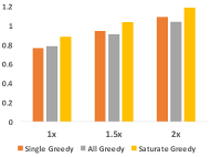
(a) Twitter100 ($k=10$)

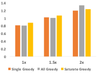
(b) Twitter250 ($k=20$)

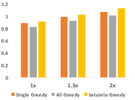
(c) Meme2000 ($k=50$)

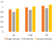
(d) Meme5000 ($k=100$)

Figure 1: Performance of the algorithms on the four topical/temporal datasets. The $x$-axis is the number of seeds selected, and the $y$-axis the resulting robust influence (compared to seed sets of size $k$).

The first main insight is that (in the instances we study) getting to over-select seeds by 50%, all three algorithms achieve a robust influence of at least 1.0. In other words, 50% more seeds let the algorithms perform as though they knew exactly which of the (adversarially chosen) diffusion settings was the true one. This suggests that the networks in our data sets share a lot of similarities that make influential nodes in one network also (mostly) influential in the other networks. This interpretation is consistent with the observation that the baseline heuristics perform similarly to (and in one case better than) the Saturate Greedy algorithm. Notice, however, that when selecting just $k$ seeds, Saturate Greedy does perform best (though only by a small margin) among the three algorithms. This suggests that keeping robustness in mind may be more crucial when the algorithm does not get to compensate with a larger number of seeds.

Results: Visualization

To further illustrate the tradeoffs between robust and non-robust optimization, we visualize the seeds selected by Saturate Greedy (robust seeds) compared to seeds selected non-robustly based on only one diffusion setting. For legibility, we focus only on the Twitter250 data set, and only plot $4$ out of the $5$ networks. (The fifth network is very sparse, and thus not particularly interesting.)

Figure 2 compares the seeds selected by Saturate Greedy with those (approximately) maximizing the influence for the Iran network. Notice that Saturate Greedy focuses mostly (though not exclusively) on the densely connected core of the network (at the center), while the Iran-specific optimization also exploits the dense regions on the left and at the bottom. These regions are much less densely connected in the US politics and Climate networks, while the core remains fairly densely connected, leading the Saturate Greedy solution to be somewhat more robust.

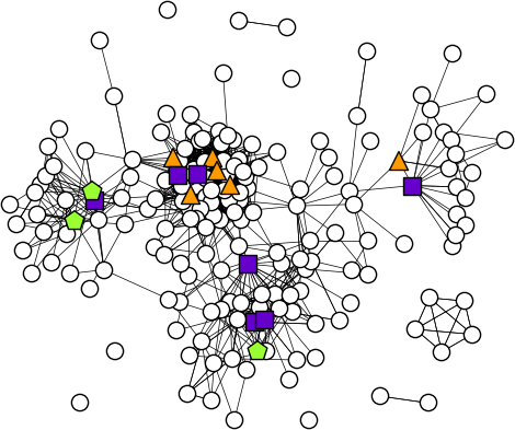
(a) Iran

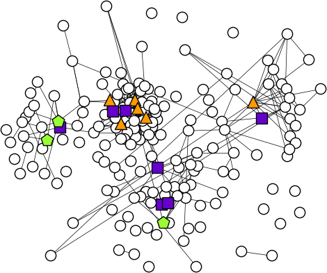
(b) Haiti

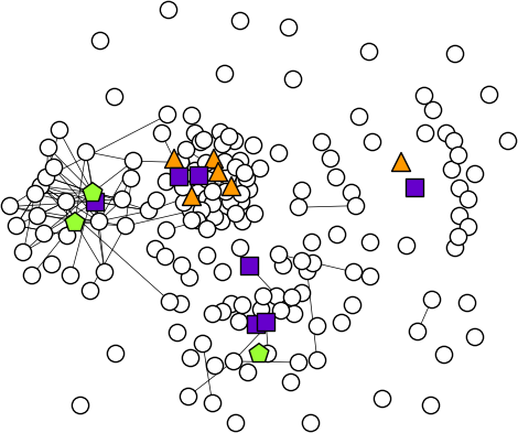
(c) US politics

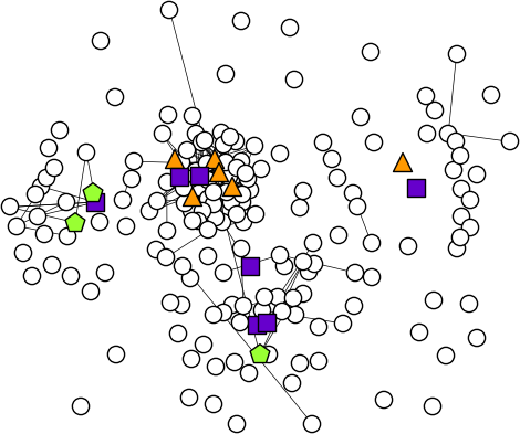
(d) Climate

Figure 2: Saturate Greedy vs. Iran graph seed nodes. Green/pentagon nodes are selected in both; orange/triangle nodes are selected by Saturate Greedy only; purple/square nodes for Iran only.

Similarly, Figure 3 compares the Saturate Greedy seeds (which are the same as in Figure 2) with seeds for the Climate network. The trend here is exactly the opposite. The seeds selected based only on the Climate network are exclusively in the core, because the other parts of the Climate network are barely connected. On the other hand, the robust solution picks a few seeds from the clusters at the bottom, left, and right, which are present in other networks. These seeds lead to extra influence in those networks, and thus more robustness.

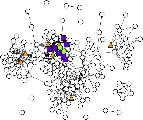
(a) Iran

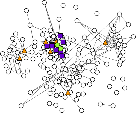
(b) Haiti

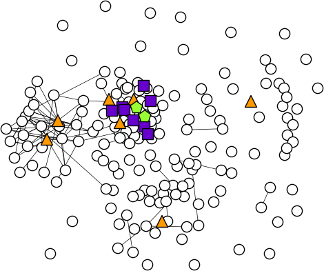
(c) US politics

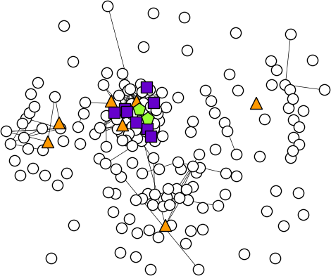
(d) Climate

Figure 3: Saturate Greedy vs. Climate graph seed nodes. Green/pentagon nodes are selected in both; orange/triangle nodes are selected by Saturate Greedy only; purple/square nodes for Climate only.

5.2 Different Diffusion Models

In choosing a diffusion model, there is little convincing empirical work guiding the choice of a model class (such as CIC, DIC, or threshold models) or of distributional assumptions for model parameters (such as edge delay). A possible solution is to optimize robustly with respect to these different possible choices.

In this section, we evaluate such an approach. Specifically, we perform two experiments: (1) learning the CIC influence network under different parametric assumptions about the delay distribution, and (2) learning the influence network under different models of influence (CIC, DIC, DLT). We again use the MemeTracker dataset, restricting ourselves to the data from August 2008 and the 500 most active users. We use the MultiTree algorithm of Gomez-Rodriguez et al. [20] to infer the diffusion network from the observed cascades. This algorithm requires a parametric assumption for the edge delay distribution. We infer ten different networks $G_{i}$ corresponding to the Exponential distribution with parameters 0.05, 0.1, 0.2, 0.5, 1.0, and to the Rayleigh distribution with parameters 0.5, 1, 2, 3, 4. The length of the observation window is set to 1.0.

We then use the three algorithms to perform robust influence maximization for $k=10$ seeds, again allowing the algorithms to exceed the target number of vertices. The influence model for each graph is the CIC model with the same parameters that were used to infer the graphs.

The performance of the algorithms is shown in Figure 4(a). All methods achieve satisfactory results in the experiment; this is again due to high similarity between the different diffusion settings inferred with different parameters.

For the second experiment, we investigate the robustness across different classes of diffusion models. We construct three instances of the DIC, DLT and DIC model from the ground truth diffusion network between the 500 active users. For the DIC model, we set the activation probability uniformly to $0.1$. For the DLT model, we follow [25] and set the edge weights to $1/d_{v}$ where $d_{v}$ is the in-degree of node $v$. For the CIC model, we use an exponential distribution with parameter $0.1$ and an observation window of length $1.0$. We perform robust influence maximization for $k=10$ seeds and again allow the algorithms to exceed the target number of seeds.

The results are shown in Figure 4(b). Similarly to the case of different estimated parameters, all methods achieve satisfactory results in the experiment due to the high similarity between the diffusion models. Our results raise the intriguing question of which types of networks would be prone to significant differences in algorithmic performance based on which model is used for network estimation.

5.3 Networks sampled from the Perturbation Interval model

To investigate the performance when model parameters can only be placed inside “confidence intervals” (i.e., the Perturbation Interval model), we carry out experiments under two networks, MemeTracker and STOCFOCS.

The MemeTracker network is extracted from the MemeTracker data set using the ConNIe algorithm [34] to infer the (fractional) parameters (activation probabilities) of a DIC model from the same 500-node MemeTracker data set used in the previous section. We also ran experiments on a multigraph extracted from co-authorship of published papers in the conferences STOC and FOCS from 1964–2001. Each node in that network is a researcher with at least one publication in one of the conferences. For each multi-author paper, we add a complete undirected graph among the authors. We compress parallel edges into a single edge with weight $w_{e}$ and set the activation probability $p_{e}=0.1\cdot w_{e}$. If $p_{e}>1$, we truncate its value to $1$. Following the approach of [24], for both networks, we assign “confidence intervals” $I_{e}=[(1-q)p_{e},(1+q)p_{e}]$, where the $p_{e}$ are the inferred activation probabilities. For experiments on the MemeTracker network, we set $q\in\{10\%,20\%,30\%,\ldots,100\%\}$, while we use a coarse grid for the experiments on the large graph STOCFOCS with $q\in\{5\%,10\%,20\%,50\%,100\%\}$.

While Lemma 1 guarantees that the worst-case instances have activation probabilities $(1-q)p_{e}$ or $(1+q)p_{e}$, this still leaves $2^{|E|}$ candidate functions, too many to include. We generate an instance for our experiments by sampling 10 of these functions uniformly, i.e., by independently making each edge’s activation probability either $(1-q)p_{e}$ or $(1+q)p_{e}$. This collection is augmented by two more instances: one where all edge probabilities are $(1-q)p_{e}$, and one where all probabilities are $(1+q)p_{e}$. Notice that with the inclusion of these two instances, the All Greedy heuristic generalizes the LUGreedy algorithm by Chen et al. [6], but might provide strictly better solutions on the selected instances because it explicitly considers those additional instances. The algorithms get to select 20 seed nodes; note that in these experiments, we are not considering a bicriteria approximation.

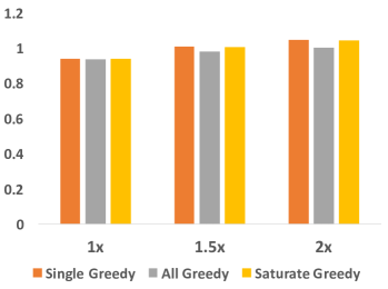
(a) Different Distributions.

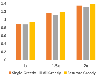
(b) Different Models

Figure 4: Performance of the algorithms (a) under different delay distributions following the CIC model, and (b) under different classes of diffusion models. The $x$-axis shows the number of seeds selected, and $k=10$.

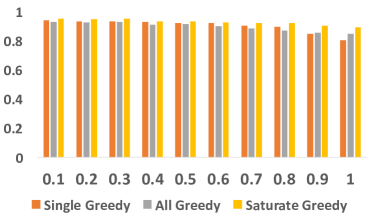
(a) Perturbation Interval model: MemeTracker ($k=20$)

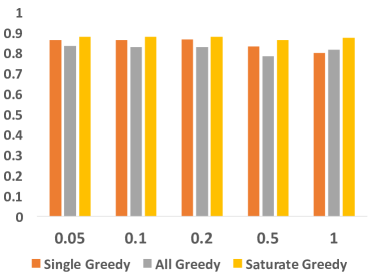
(b) Perturbation Interval model: STOCFICS ($k=50$)

Figure 5: Performance of the algorithms under networks sampled from the Perturbation Interval model: (a) MemeTracker networ; (b) STOCFOCS network. (the $x$ axis shows the (relative) size of the perturbation interval $I_{e}$).

The results are shown in Figures 5(a) and 5(b). Contrary to the previous results, when there is a lot of uncertainty about the edge parameters (relative interval size 100% in both networks), the Saturate Greedy algorithm more clearly outperforms the Single Greedy and All Greedy heuristics. Thus, robust optimization does appear to become necessary when there is a lot of uncertainty about the model’s parameters.

Notice that the evaluation of the algorithms’ seed sets is performed only with respect to the sampled influence functions, not with respect to all $2^{|E|}$ functions. Whether one can efficiently identify a worst-case parameter setting for a given seed set $S_{0}$ is an intriguing open question. Absent this ability, we cannot efficiently guarantee that the solutions are actually good with respect to all parameter settings.

5.4 Scalability

To evaluate the scalability of the algorithms, we depart from real-world data sets in order to obtain a controlled environment. We generate networks using the Kronecker graph model [30] with either random, core-peripheral or hierarchical-community structures. For each type, we generate a set of $5,10,15,20,25$ networks of sizes $128,256,\ldots,4096$. We use the DIC model with activation probability set to $0.1$, and select $k=50$ nodes. The running times of the three algorithms are shown in Figure 6 and Figure 7. In Figure 6, we fix the number of networks to five and vary the size of each network; in Figure 7, we fix the size of the networks to $1024$ and vary the number of networks. The graphs show that the heuristics are faster than the Saturate Greedy algorithm by about a factor of ten, but all three algorithms scale linearly both in the size of the graph and the number of networks, due to the fast influence estimation method.

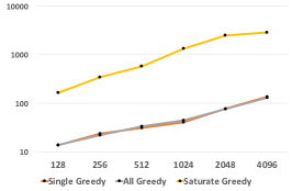
(a) Random

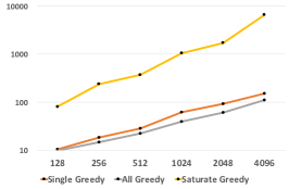
(b) Core-peripheral

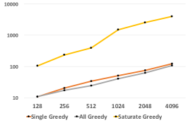
(c) Hierarchical-community

Figure 6: Running times on Kronecker graph networks with different structures. The $x$ axis represents the number of nodes, and the $y$-axis is the running time in seconds, both plotted on a log scale.

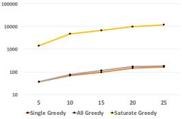
(a) Random

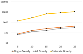
(b) Core-peripheral

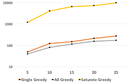
(c) Hierarchical-community

Figure 7: Running times on Kronecker graph networks with different structures. The $x$ axis represents the number of diffusion settings, and the $y$-axis is the running time in seconds, both plotted on a log scale.

6 Future Work

Our work marks an early step, rather than the conclusion, in devising robust algorithms for social network tasks, and more specifically Influence Maximization. An interesting unresolved question is whether one can efficiently find an (approximately) worst-case influence function in the Perturbation Interval model. This would allow us to empirically evaluate the performance of natural heuristics for the Perturbation Interval model, such as randomly sampling a small number of influence functions. Furthermore, it would allow us to design “column generation” style algorithms for the Perturbation Interval model, where we alternate between finding a near-optimal seed set for all influence functions encountered so far, and finding a worst-case influence function for the current seed set, which will then be added to the encountered functions.

In the context of the bigger agenda, one could conceive of other notions of robustness in Influence Maximization, perhaps tracing a finer line between worst-case and Bayesian models. Also, much more research is needed into identifying which influence models best capture the behavior of real-world cascades, and under what circumstances. It is quite likely that different models will perform differently depending on the type of cascade and many other factors, and in-depth evaluations of the models could give practitioners more guidance on which mathematical models to choose. While our model of robustness allows us to combine instances of different models (e.g., IC and LT), this may come at a cost of decreased performance for each of the models individually. Thus, it remains an important task to identify the influence models that best fit real-world data.

Acknowledgments

We would like to thank Shaddin Dughmi for useful pointers and feedback, and Shishir Bharathi and Mahyar Salek for useful discussions, and anonymous reviewers for useful feedback. The research was sponsored in part by NSF research grant IIS-1254206 and by the U.S. Defense Advanced Research Projects Agency (DARPA) under Social Media in Strategic Communication (SMISC) program, Agreement Number W911NF-12-1-0034. The views and conclusions are those of the authors and should not be interpreted as representing the official policies of the funding agency, or the U.S. Government.

Appendix A Proof of Theorem 2

We prove the two parts of the theorem by (slightly different) reductions from the gap version of Set Cover. A Set Cover instance consists of a universe $U=\{a_{1},\ldots,a_{N}\}$, a collection $\mathcal{T}$ of $M$ subsets of $U$, and an integer $k$. A set cover is a collection $\mathcal{C}\subseteq\mathcal{T}$ such that $\bigcup_{T\in\mathcal{C}}T=U$. Without loss of generality, we assume that each element is contained in at least one set — otherwise, there trivially is no set cover. Also, without loss of generality, we assume that $k\leq\min(M,N)$, as otherwise, one can trivially pick all sets or one designated set per element.

The gap version of Set Cover then asks us to decide whether there is a set cover $\mathcal{C}$ of size $|\mathcal{C}|\leq k$ or whether each set cover has size at least $(1-\delta)\ln N\cdot k$. (The algorithm is promised that the minimum size will never lie between these two values.) Dinur and Steurer [12, Corollary 1.5] showed that the gap version of Set Cover is NP-hard.

Part 1

Based on the Set Cover instance, we construct the following instance of Robust Influence Maximization under the DIC model. Let $m:=(\max(N,M))^{3/\epsilon}$. The instance consists of $N$ bipartite graphs on a shared vertex set $V=X\cup Y$. $X$ contains one node $x_{T}$ for each set $T\in\mathcal{T}$; $Y$ contains $m$ nodes $y_{a,1},\ldots,y_{a,m}$ for each element $a\in U$. Hence, the number of nodes in the constructed graph is $n=M+mN=\Theta(mN)\leq\Theta(m^{1+\epsilon/3})$; in particular, it is polynomial, and the reduction takes polynomial time.

In the ${i}^{\rm th}$ influence function, all nodes $x_{T}$ with $T\ni a_{i}$ have a directed edge with activation probability 1 (or exponential delay distribution with delay parameter 1) to all of the $y_{a_{i},j}$ (for all $j$); no other edges are present. Hence, $|\Sigma|=N$, and $\ln N=\ln|\Sigma|$. For the CIC model, the time window has size $T=NM$.

First, consider the case when there is a set cover $\mathcal{C}$ of size $k$. Choose the corresponding $x_{T},T\in\mathcal{C}$ as seed nodes, and call the resulting seed set $S$. Because $\mathcal{C}$ is a set cover, in the ${i}^{\rm th}$ instance, all of the $y_{a_{i},j}$ are activated, for a total of at least $m+k$ nodes. (Under the CIC model, all of these $y_{a_{i},j}$ are activated with high probability, not deterministically, within the $T$ steps) Because none of the nodes in $X$ and none of the $y_{a_{i^{\prime}},j},i^{\prime}\neq i$ have incoming edges in the ${i}^{\rm th}$ instance, the optimum solution for that instance can activate at most all of the $m$ nodes $y_{a_{i},j}$ and its $k$ selected nodes, for a total of $m+k$. Thus, the objective function value will be 1 (or arbitrarily close to 1 w.h.p. for the CIC model).

Now assume that there is no set cover of size $(1-\delta)\ln N\cdot k$, and consider any seed set $S$. Let $k^{\prime}=|S\cap X|\leq(1-\delta)\ln N\cdot k$ be the number of nodes from $X$ selected as seeds. Because the set $\mathcal{S}:=\{T\in\mathcal{T}\;|\;x_{T}\in S\}$ cannot be a set cover by assumption, there must be some $a_{i}\notin\bigcup_{T\in\mathcal{S}}T$. Therefore, under the the ${i}^{\rm th}$ influence function, none of the $y_{a_{i},j}$ can be ever activated, except those selected directly in $S$. Hence, the number of nodes activated under the ${i}^{\rm th}$ influence function is at most $|S|\leq(1-\delta)\ln N\cdot k$. On the other hand, by selecting just one node $x_{T}$ corresponding to any set $T\ni a_{i}$, one could have activated all of the $y_{a_{i},j}$ (with high probability under the CIC model), for a total of $m$. Thus, the objective function value is at most $\rho(S)\leq\frac{(1-\delta)\ln N\cdot k}{m}\leq O(m^{2\epsilon/3-1})\leq O(n^{\frac{2\epsilon-3}{3+\epsilon}})=o(n^{-(1-\epsilon)})$, where we crudely bounded both $\ln N$ and $k$ by $N\leq O(m^{\epsilon/3})$.

Hence, a $((1-\delta)\ln N,O(n^{1-\epsilon}))$ bicriteria approximation algorithm could distinguish the two cases, and thus solve the gap version of Set Cover.

Part 2

For the second part, we just consider the gap version with a fixed $\delta$, say, $\delta=\frac{1}{2}$. Then, in the hard instances, $M$ and $N$ are polynomially related, which we assume here, i.e., $M\leq N^{q}$ for some constant $q$ which is independent of $\epsilon$ or $N$.

Based on the Set Cover instance, we construct a different Robust Influence Maximization instance, consisting of a directed graph with three layers $V=X\cup Y\cup Z$. The first layer again contains one node $x_{T}$ for each set $T\in\mathcal{T}$; the second layer now contains just one node $y_{a}$ for each element $a\in U$. There is an edge (with known influence probability 1, or exponential delay distribution with parameter 1) from $x_{T}$ to $y_{a}$ if and only if $a\in T$. The third layer $Z$ contains $m=(\max(N,M))^{2/\epsilon}$ nodes. For each $a\in U$ and $z\in Z$, there is a directed edge $(y_{a},z)$ with complete uncertainty about its parameter: under the DIC model, the probability is in the interval $I_{(y_{a},z)}=[0,1]$, and under the CIC model, the edge delay is exponentially distributed with parameter in the interval $I_{(y_{a},z)}=(0,1]$. In total, the graph has $n=N+M+m=\Theta(m)$ nodes (in particular, polynomially many), and the reduction takes polynomial time. Because $N$ is at most polynomially smaller than $M$, we have $N=\Omega(n^{\epsilon/2q})$, and thus $\ln N=\Omega(\frac{\epsilon}{q}\cdot\ln(n))$. For the CIC model, we set the time horizon to $T=NM$.

First, consider the case when there is a set cover $\mathcal{C}$ of size $k$. Consider choosing the corresponding $x_{T},T\in\mathcal{C}$ as seed nodes; call the resulting seed set $S$. $S$ will definitely activate all nodes in $Y$, for a total of $k+N$. Now, consider any assignment of probabilities $p_{y_{a},z}$ or edge delays $\Delta_{y_{a},z}$ to the edges from $Y$ to $Z$, and an optimal seed set $S^{*}$ of size $k$. Let $Z^{*}=Z\cap S^{*}$ be the set of seed nodes chosen from $Z$, of size $k^{\prime}$. Then, $S^{*}$ definitely activates all of $Z^{*}$, and at most all $N$ nodes from $Y$ as well as $k-k^{\prime}$ nodes from $X$, for a total (so far) of $N+k$. For any node $z\in Z\setminus Z^{*}$, the probability that it is activated by $S$ is at least as large as under $S^{*}$, because for any values of the individual activation probabilities or delays between $Y$ and $Z$, the fact that $S$ activates all of $Y$ ensures that any node in $Z$ activated under $S^{*}$ is also activated under $S$ (by time $T$, in the case of the CIC model). Because, the expected number of nodes activated from $Z\setminus Z^{*}$ is at least as large under $S$ as under $S^{*}$, and the ratio is $1$. Since this holds for all settings of the activation probabilities or edge delay parameters, we get that $\rho(S)\geq 1$.

Now assume that there is no set cover of size $\frac{1}{2}\ln N\cdot k$, and consider any seed set $S$. If $S$ contained any node $y_{a}$, we could replace it with any node $x_{T}$ such that $a\in T$ and activate at least as many nodes as before, so assume without loss of generality that $S\cap Y=\emptyset$. Because $|S\cap X|\leq|S|\leq\frac{1}{2}\ln N\cdot k$, the gap guarantee implies that there is at least one node $y_{a}\in Y$ that is never activated by $S$. Now consider the probability assignment $p_{y_{a},z}=1$ for all $z\in Z$, and $p_{y,z}=0$ for all $y\neq y_{a},z\in Z$. (Under the CIC model, set $\Delta_{y_{a},z}=1$ for all $z\in Z$, and $\Delta_{y,z}=1/(NM)^{2}$ for all $y\neq y_{a},z\in Z$.) Then, the seed set $S$ cannot activate any nodes in $Z$ (except those it may have selected), and will activate a total of at most $N+k=O(N)=O(n^{\epsilon/2})$ nodes. (Under the CIC model, this statement holds with high probability.) On the other hand, the seed set $\{y_{a}\}$ (just a single node) would have activated all of $Z$ (with high probability, under the CIC model), for a total of $m+1=\Omega(n)$ nodes. Hence, the ratio is at most $O(n^{\epsilon/2}/n)=O(1/n^{1-\epsilon/2})$, implying that $\rho(S)\leq O(1/n^{1-\epsilon/2})$.

If there were an $(\epsilon\cdot c\cdot\ln(n),O(n^{1-\epsilon}))$ bicriteria approximation algorithm for a sufficiently small constant $c$, it could distinguish which of the two cases ($\rho(S)=1,\rho(S)\leq O(1/n^{1-\epsilon/2})$) applied, thus solving the gap version of Set Cover.

References

- [1] Bruno Abrahao, Flavio Chierichetti, Robert Kleinberg, and Alessandro Panconesi. Trace complexity of network inference. In Proc. 19th Intl. Conf. on Knowledge Discovery and Data Mining, pages 491–499, 2013.
- [2] Abhijin Adiga, Chris J. Kuhlman, Henning S. Mortveit, and Anil Kumar S. Vullikanti. Sensitivity of diffusion dynamics to network uncertainty. In Proc. 28th AAAI Conf. on Artificial Intelligence, 2013.
- [3] Christian Borgs, Michael Brautbar, Jennifer Chayes, and Brendan Lucier. Maximizing social influence in nearly optimal time. In Proc. 25th ACM-SIAM Symp. on Discrete Algorithms, pages 946–957, 2014.
- [4] Karen E. Campbell and Barrett A. Lee. Name generators in surveys of personal networks. Social Networks, 13(3):203–221, 1991.
- [5] Wei Chen, Laks V.S. Lakshmanan, and Carlos Castillo. Information and Influence Propagation in Social Networks. Synthesis Lectures on Data Management. Morgan & Claypool, 2013.
- [6] Wei Chen, Tian Lin, Zihan Tan, Mingfei Zhao, and Xuren Zhou. Robust influence maximization. In Proc. 22nd Intl. Conf. on Knowledge Discovery and Data Mining, 2016.
- [7] Wei Chen, Yajun Wang, and Siyu Yang. Efficient influence maximization in social networks. In Proc. 15th Intl. Conf. on Knowledge Discovery and Data Mining, pages 199–208, 2009.
- [8] Wei Chen, Yajun Wang, Yang Yuan, and Qinshi Wang. Combinatorial multi-armed bandit and its extension to probabilistically triggered arms. J. Mach. Learn. Res., 17(1):1746–1778, 2016.
- [9] Wei Chen, Yifei Yuan, and Li Zhang. Scalable influence maximization in social networks under the linear threshold model. In Proc. 10th Intl. Conf. on Data Mining, pages 88–97, 2010.
- [10] Xiaodong Chen, Guojie Song, Xinran He, and Kunqing Xie. On influential nodes tracking in dynamic social networks. In Proc. 15th SIAM Intl. Conf. on Data Mining, pages 613–621, 2015.
- [11] Hadi Daneshmand, Manuel Gomez-Rodriguez, Le Song, and Bernhard Schölkopf. Estimating diffusion network structures: Recovery conditions, sample complexity & soft-thresholding algorithm. In Proc. 31st Intl. Conf. on Machine Learning, 2014.
- [12] Irit Dinur and David Steurer. Analytical approach to parallel repetition. In Proc. 45th ACM Symp. on Theory of Computing, pages 624–633, 2014.
- [13] Pedro Domingos and Matthew Richardson. Mining the network value of customers. In Proc. 7th Intl. Conf. on Knowledge Discovery and Data Mining, pages 57–66, 2001.
- [14] Nan Du, Yingyu Liang, Maria-Florina Balcan, and Le Song. Influence function learning in information diffusion networks. In Proc. 31st Intl. Conf. on Machine Learning, 2014.
- [15] Nan Du, Le Song, Manuel Gomez-Rodriguez, and Hongyuan Zha. Scalable influence estimation in continuous-time diffusion networks. In Proc. 25th Advances in Neural Information Processing Systems, 2013.
- [16] Jacob Goldenberg, Barak Libai, and Eitan Muller. Talk of the network: A complex systems look at the underlying process of word-of-mouth. Marketing Letters, 12:211–223, 2001.
- [17] Jacob Goldenberg, Barak Libai, and Eitan Muller. Using complex systems analysis to advance marketing theory development: Modeling heterogeneity effects on new product growth through stochastic cellular automata. Academy of Marketing Science Review, 2001.
- [18] Manuel Gomez-Rodriguez, David Balduzzi, and Bernhard Schölkopf. Uncovering the temporal dynamics of diffusion networks. In Proc. 28th Intl. Conf. on Machine Learning, pages 561–568, 2011.
- [19] Manuel Gomez-Rodriguez, Jure Leskovec, and Andrease Krause. Inferring networks of diffusion and influence. ACM Transactions on Knowledge Discovery from Data (TKDD), 5(4):21, 2012.
- [20] Manuel Gomez-Rodriguez and Bernhard Schölkopf. Submodular inference of diffusion networks from multiple trees. In Proc. 29th Intl. Conf. on Machine Learning, 2012.
- [21] Amit Goyal, Francesco Bonchi, and Laks V. S. Lakshmanan. A data-based approach to social influence maximization. Proc. VLDB Endowment, 5(1):73–84, 2011.
- [22] Amit Goyal, Francesco Bonchi, Laks V. S. Lakshmanan, and Suresh Venkatasubramanian. On minimizing budget and time in influence propagation over social networks. Social Network Analysis and Mining, 3(2):179–192, 2013.
- [23] Mark Granovetter. Threshold models of collective behavior. American Journal of Sociology, 83:1420–1443, 1978.
- [24] Xinran He and David Kempe. Stability of influence maximization. Unpublished Manuscript, available at \urlhttp://arxiv.org/abs/1501.04579, 2015.
- [25] David Kempe, Jon Kleinberg, and Eva Tardos. Maximizing the spread of influence in a social network. Theory of Computing, 11(4):105–147, 2015. A preliminary version of the results appeared in KDD 2003 and ICALP 2005.
- [26] Sanjeev Khanna and Brendan Lucier. Influence maximization in undirected networks. In Proc. 25th ACM-SIAM Symp. on Discrete Algorithms, pages 1482–1496, 2014.
- [27] Andreas Krause, H. Brendan McMahan, Carlos Guestrin, and Anupam Gupta. Robust submodular observation selection. In Journal of Machine Learning Research, volume 9, pages 2761–2801, 2008.
- [28] Siyu Lei, Silviu Maniu, Luyi Mo, Reynold Cheng, and Pierre Senellart. Online influence maximization. In Proc. 21st Intl. Conf. on Knowledge Discovery and Data Mining, pages 645–654, 2015.
- [29] Jure Leskovec, Lars Backstrom, and Jon Kleinberg. Meme-tracking and the dynamics of the news cycle. In Proc. 15th Intl. Conf. on Knowledge Discovery and Data Mining, pages 497–506, 2009. Note: updated data sets at http://www.memetracker.org/.
- [30] Jure Leskovec, Deepayan Chakrabarti, Jon Kleinberg, Christos Faloutsos, and Zoubin Ghahramani. Kronecker graphs: An approach to modeling networks. Journal of Machine Learning Research, 11:985–1042, 2010.
- [31] Jure Leskovec, Andreas Krause, Carlos Guestrin, Christos Faloutsos, Jeanne VanBriesen, and Natalie S. Glance. Cost-effective outbreak detection in networks. In Proc. 13th Intl. Conf. on Knowledge Discovery and Data Mining, pages 420–429, 2007.
- [32] Meghna Lowalekar, Pradeep Varakantham, and Akshat Kumar. Robust influence maximization (extended abstract). In Proc. 15th Intl. Conf. on Autonomous Agents and Multiagent Systems, pages 1395–1396, 2016.
- [33] Elchanan Mossel and Sebastien Roch. Submodularity of influence in social networks: From local to global. SIAM Journal on Computing, 39(6):2176–2188, 2010.
- [34] Seth A. Myers and Jure Leskovec. On the convexity of latent social network inference. In Proc. 22nd Advances in Neural Information Processing Systems, pages 1741–1749, 2010.
- [35] Harikrishna Narasimhan, David C. Parkes, and Yaron Singer. Learnability of influence in networks. In Proc. 27th Advances in Neural Information Processing Systems, pages 3168–3176, 2015.
- [36] George L. Nemhauser, Laurence A. Wolsey, and Marshall L. Fisher. An analysis of the approximations for maximizing submodular set functions. Mathematical Programming, 14:265–294, 1978.
- [37] Praneeth Netrapalli and Sujay Sanghavi. Learning the graph of epidemic cascades. In ACM SIGMETRICS Performance Evaluation Review, pages 211–222, 2012.
- [38] Matthew Richardson and Pedro Domingos. Mining knowledge-sharing sites for viral marketing. In Proc. 8th Intl. Conf. on Knowledge Discovery and Data Mining, pages 61–70, 2002.
- [39] Kazumi Saito, Masahiro Kimura, Kouzou Ohara, and Hiroshi Motoda. Selecting information diffusion models over social networks for behavioral analysis. In Proc. 2010 European Conference on Machine Learning and Knowledge Discovery in Databases: Part III, ECML/PKDD 10, pages 180–195, 2010.
- [40] Chi Wang, Wei Chen, and Yajun Wang. Scalable influence maximization for independent cascade model in large-scale social networks. Data Mining and Knowledge Discovery Journal, 25(3):545–576, 2012.
- [41] Yu Wang, Gao Cong, Guojie Song, and Kunqing Xie. Community-based greedy algorithm for mining top- influential nodes in mobile social networks. In Proc. 16th Intl. Conf. on Knowledge Discovery and Data Mining, pages 1039–1048, 2010.