Work-Efficient Parallel and Incremental Graph Connectivity

Abstract

On an evolving graph that is continuously updated by a high-velocity stream of edges, how can one efficiently maintain if two vertices are connected? This is the connectivity problem, a fundamental and widely studied problem on graphs. We present the first shared-memory parallel algorithm for incremental graph connectivity that is both provably work-efficient and has polylogarithmic parallel depth. We also present a simpler algorithm with slightly worse theoretical properties, but which is easier to implement and has good practical performance. Our experiments show a throughput of hundreds of millions of edges per second on a $20$-core machine.

1 Introduction

Graph connectivity is a fundamental problem with a long history. On an undirected graph, the basic connectivity question is: given two vertices, is there a path between them?

Our work is motivated by the need for high throughput real-time streaming graph analytics. Every minute, a staggering amount of high-velocity linked data is being generated from social media interactions, the Internet of Things (IoT) devices, among others—and timely insights from them are much sought after. These data are usually cast as a stream of edges with the goal of maintaining certain local and global properties on the accumulated data. Modern stream processing systems such as IBM Infosphere Streams [10] and Apache Spark [19] rely on parallel processing of input streams to achieve high throughput and real-time analytics. However, these systems only provide the software infrastructure; scalable, parallel, and dynamic graph algorithms are still needed to make use of the potential of these systems.

As a first step towards efficient parallel and dynamic graph algorithms, we consider the parallel incremental graph connectivity problem in a setting where edges and queries arrive in bulk. Tackling the parallel incremental version of the problem, which allows only addition of edges to the graph, is an important stepping stone towards the more general problem of (fully) dynamic connectivity that allows both addition and deletion of edges.

There exist sequential algorithms for incremental graph connectivity, starting from the popular union-find data structure [18]; but these are, for the most part, unable to take advantage of parallelism. There exist parallel algorithms for graph connectivity (e.g., [17, 9]), but these are, for the most part, not incremental. None of these meet the need for high throughput dynamic graph processing.

In order to make effective use of parallelism in stream processing, systems such as Apache Spark [19] use a model of “discretized streams”, where the incoming high-volume stream is divided into a sequence of “minibatches”. Each minibatch is processed using a parallel computation, and the resulting system can potentially achieve a very high throughput, subject to the availability of appropriate algorithms. We adopt this model in our work and seek parallel methods that can process a minibatch of edges efficiently.

Model: On a vertex set $V$, a graph stream $\mathcal{A}$ is a sequence of minibatches $A_{1},A_{2},\dots$, where each minibatch $A_{i}$ is a set of edges on $V$. The graph at the end of observing $A_{t}$, denoted by $G_{t}$, is $G_{t}=(V,\cup_{i=1}^{t}A_{i})$ containing all the edges up to $t$. The minibatches $A_{i}$ need not be of equal sizes.

In this paper, we study a bulk-parallel incremental connectivity problem, which is to maintain a data structure that provides two operations: Bulk-Update and Bulk-Query. The Bulk-Update operation takes as input a minibatch of edges $A_{i}$ and adds them to the graph. The Bulk-Query operation takes a minibatch of vertex-pair queries and returns for each query, whether the two vertices are connected on the edges observed so far in the stream. On this data structure, the Bulk-Query and Bulk-Update operations are each invoked with a (potentially large) minibatch of input, each processed using a parallel computation. But a bulk operation, say a Bulk-Update, must complete before the next operation, say a Bulk-Query, can begin.

Contributions: We present the first shared-memory parallel algorithm for incremental connectivity that is both provably work-efficient and has polylogarithmic parallel depth. We make the following specific contributions:

—

Simple Parallel Incremental Connectivity. We first present a simple algorithm that is easy to implement, yet has good theoretical properties. On a graph with $n$ vertices, this algorithm makes a single pass through the stream using $O(n)$ memory, and can process a minibatch of $b$ edges, using $O(b\log n)$ work and $O(\mathop{\mathrm{polylog}}(n))$ parallel depth. We describe this algorithm in Section 4.

—

Work-Efficient Parallel Incremental Connectivity. We present an improved parallel algorithm with total work $O((m+q)\alpha(m+q,n))$ where $m$ is the total number of edges across all minibatches, $q$ is the total number of connectivity queries across all minibatches, and $\alpha$ is an inverse Ackermann’s function (see Section 2). This matches the work of the best sequential counterpart, which makes this parallel algorithm work-efficient. Further, the parallel depth of processing a minibatch is polylogarithmic. Hence, the sequential bottleneck in the runtime of the parallel algorithm is very small, and the algorithm is capable of using almost a linear number of processors efficiently. We are not aware of a prior parallel algorithm with such provable properties on work and depth. We describe this algorithm in Section 5.

—

Implementation and Evaluation. We implemented and benchmarked a variation of our simple parallel algorithm on a shared-memory machine. Our experimental results show that the algorithm achieves good speedups in practice and is able to efficiently use the available parallelism. On a 20-core machine, it can process hundreds of millions of edges per second, and realize a speedup of $8$–$11$x over its single threaded performance. Further analysis shows good scalability properties as the number of threads is varied. We describe this in Section 6.

2 Related Work

Let $n$ be the number of vertices, $m$ the number of operations, and $\alpha$ an inverse Ackermann’s function (very slow-growing, practically a constant independent of $n$). In the sequential setting, the basic data structure for incremental connectivity is the well-studied union-find data structure [5]. Tarjan [18] achieves an $O(\alpha(m,n))$ amortized time per find, which has been shown to be optimal (see Seidel and Sharir [15] for an alternate analysis).

Recent work on streaming graph algorithms focuses on minimizing the memory requirement, with little attention given to the use of parallelism. This line of work has largely focused on the “semi-streaming model” [8], which allows $O(n\cdot\mathop{\mathrm{polylog}}(n))$ space usage. In this model, the union-find data structure [18] solves incremental connectivity in $O(n)$ space and a total time nearly linear in $m$.

When only $o(n)$ of workspace (sublinear) is allowed, interesting tradeoffs are known for multi-pass algorithms. For an allotment of $O(s)$ workspace, an algorithm needs $\Omega(n/s)$ passes [8] to compute the connected components of a graph. Demetrescu et al. [7] consider the W-stream model, which allows the processing of streams in multiple passes in a pipelined manner: the output of the $i$-th pass is given as input to the $(i+1)$-th pass. They show a tradeoff between the number of passes and the memory required. With $s$ bits of space, their algorithm computes connected components in $O((n\log n)/s)$ passes. Demetrescu et al. [6] present a simulation of a PRAM algorithm on the W-Stream model, allowing existing PRAM algorithms to run sequentially in the W-Stream model.

McColl et al. [13] present a parallel algorithm for maintaining connected components in a fully dynamic graph, which handles edge deletions—a more general setting than ours. As part of a bigger project (STINGER), their work focuses on engineering algorithms that work well on real-world graphs and gives no theoretical analysis of the parallel complexity. In contrast, this work focuses on achieving the best theoretical efficiency, matching the work of the best sequential counterpart.

Berry et al. [2] present methods for maintaining connected components in their parallel graph stream model, called X-Stream, which periodically ages out edges. Their algorithm is essentially an “unrolling” of the algorithm of [7], and edges are passed from one processor to another until the connected components are found by the last processor in the sequence. Compared to our work, the input model and notions of correctness differ. Our work views the input stream a sequence of batches, each a set of edges or a set of queries, which are unordered within the set. Their algorithm strictly respects the sequential ordering the edges and queries. Further, they age out edges (we do not). Also, they do not give provable parallel complexity bounds.

There are multiple parallel (batch) algorithms for graph connectivity including [17, 9] that are work-efficient (linear in the number of edges) and that have polylogarithmic depth. Prior work on wait-free implementations of the union-find data structure [1] focuses on the asynchronous model, where the goal is to be correct under all possible interleavings of operations; unlike us, they do not focus on bulk processing of edges. There is also a long line of work on sequential algorithms for maintaining graph connectivity on an evolving graph. See the recent work by [12] that addresses this problem in the general dynamic case and the references therein.

3 Preliminaries and Notation

Throughout the paper, let $[n]$ denote the set $\{0,1,\dots,n\}$. A sequence is written as $X=\langle x_{1},x_{2},\dots,x_{|X|}\rangle$, where $|X|$ denotes the length of the sequence. For a sequence $X$, the $i$-th element is denoted by $X_{i}$ or $X[i]$. Following the set-builder notation, we denote by $\langle f(x)\,:\,\Phi(x)\rangle$ a sequence generated (logically) by taking all elements that satisfy $\Phi(x)$, preserving their original ordering, and transform them by applying $f$. For example, if $T$ is a sequence of numbers, the notation $\langle 1+f(x)\,:\,x\in T\text{ and }x\text{ odd}\rangle$ means a sequence created by taking each element $x$ from $T$ that are odd and map $x$ to $1+f(x)$, retaining their original ordering. Furthermore, we write $S\oplus T$ to mean the concatenation of $S$ and $T$.

We design algorithms in the work-depth model assuming an underlying CRCW PRAM machine model. As is standard, the work of an algorithm is the total operation count, and the depth (also called parallel time or span) is the length of the longest chain of dependencies within a parallel computation. The gold standard for algorithms in this model is to perform the same amount of work as the best sequential counterpart (work efficient) and to have polylogarithmic depth. We remark that an algorithm designed for the CRCW model can work in other shared memory models such as EREW PRAM, with a depth that is a logarithmic factor worse.

We use standard parallel operations such as filter, prefix sum, map (applying a constant-cost function), and pack, all of which has $O(n)$ work and at most $O(\log^{2}(n))$ depth on an input sequence of length $n$. Given a sequence of $m$ numbers, there is a duplicate removal algorithm removeDup running in $O(m)$ work and $O(\log^{2}m)$ depth [11]. We also use the following results to sort integer keys in a small range faster than a typical comparison-based algorithm:

Theorem 1 (Parallel Integer Sort [14]).

There is an algorithm intSort that takes a sequence of integer keys $a_{1},a_{2},\dots,a_{n}$, each a number between $0$ and $c\cdot{}n$, where $c=O(1)$, and produces a sorted sequence in $O(n)$ work and $\mathop{\mathrm{polylog}}(n)$ depth.

Parallel Connectivity: For a graph $G=(V,E)$, a connected component algorithm (CC) computes a sequence of connected components of $G$ $\langle C_{i}\rangle_{i=1}^{k}$, where each $C_{i}$ is a list of vertices in the component. There are algorithms for CC that have $O(|V|+|E|)$ work and $O(\mathop{\mathrm{polylog}}(|V|,|E|))$ depth (e.g., [9, 17]), with Gazit’s algorithm [9] requiring $O(\log|V|)$ depth.

4 Simple Bulk-Parallel Data Structure

This section describes a simple bulk-parallel data structure for incremental graph connectivity. We describe theoretical improvements to this basic version in the next section. As before, $n$ is the number of vertices in the graph stream. The main result for this section is as follows:

Theorem 2.

There is a bulk-parallel data structure for incremental connectivity, given by Algorithms Simple-Bulk-Query and Simple-Bulk-Update, where

1. The total memory consumption is $O(n)$ words.

2. A minibatch of $b$ edges is processed by Simple-Bulk-Update in $O(\log(\min\{b,n\}))$ parallel depth and $O(b\log n)$ total work.

3. A minibatch of $q$ connectivity queries, each asking for connectivity between two vertices, is answered by Simple-Bulk-Query in $O(\log n)$ parallel depth and $O(q\log n)$ total work.

In a nutshell, we show how to bootstrap a standard union-find structure to take advantage of parallelism while preserving the height of the union-find forest to be at most $O(\log n)$. For concreteness, we will work with union by size, though other variants (e.g., union by rank) will also work.

Union-Find: We review a basic union-find implementation that uses union by size. From the viewpoint of graph connectivity, union-find maintains connectivity information about a graph with vertices $V=[n]$ supporting:

• for $u\in V$, $\mbox{{find}}(u)\in V$ returns an identifier of the connected component that $u$ belongs to. This has the property that $\mbox{{find}}(u)=\mbox{{find}}(v)$ if and only if $u$ and $v$ are connected in the graph.

• for $u,v\in V$, $\mbox{{union}}(u,v)$ links $u$ and $v$ together, making them in the same connected component. It also returns the identifier of the component that both $u$ and $v$ now belong to—this is the same identifier one would get from running $\mbox{{find}}(u)$ or $\mbox{{find}}(v)$ at this point.

Conceptually, this data structure maintains a union-find forest, one tree for each connected component. In this view, $\mbox{{find}}(u)$ returns the vertex that is the root of the tree containing $u$ and $\mbox{{union}}(u,v)$ joins together the roots of the tree containing $u$ and the tree containing $v$. The trees in a union-find forest are typically represented by remembering each node’s parent, in an array parent of length $n$, where $\mbox{{parent}}[u]$ is the tree’s parent of $u$ or $\mbox{{parent}}[u]=u$ if it is the root of its component.

The running time of the union and find operations depends on the maximum height of a tree in the union-find forest. To keep the height small, at most $O(\log n)$, a simple strategy, known as union by size, is for union to always link the tree with fewer vertices into the tree with more vertices. The data structure also keeps an array for the sizes of the trees. The following results are standard (see [15], for example):

Lemma 3 (Sequential Union-Find).

On a graph with vertices $[n]$, a sequential union-find data structure implementing the union-by-size strategy consumes $O(n)$ space and has the following characteristics:

• Every union-find tree has height $O(\log n)$ and each find takes $O(\log n)$ sequential time.

• Given two distinct roots $u$ and $v$, the operation $\mbox{{union}}(u,v)$ implementing union by size takes $O(1)$ sequential time.

Our data structure maintains an instance of this union-find data structure, called $U$. Notice that the find operation is read-only. Unlike the more sophisticated variants, this version of union-find does not perform path compression.

4.1 Answering Connectivity Queries in Parallel

Connectivity queries can be easily answered in parallel, using read-only finds on $U$. To answer whether $u$ and $v$ are connected, we compute $U.\mbox{{find}}(v)$ and $U.\mbox{{find}}(u)$, and report if the results are equal. To answer multiple queries in parallel, we note that because the finds are read-only, we can answer all queries simultaneously independently of each other. We present Simple-Bulk-Query in Algorithm 1.

Input: $U$ is the union find structure, and $(u_{i},v_{i})$ is a pair of vertices, for $i=1,\ldots,q$.

Output: For each $i$, whether or not $u_{i}$ is connected to $v_{i}$ in the graph.

1

2for $i=1,2,\dots,q$ do in parallel

3       $a_{i}\leftarrow(U.\mbox{{find}}(u_{i})==U.\mbox{{find}}(v_{i}))$

4      

5return $\langle a_{1},a_{2},\ldots,a_{q}\rangle$

Algorithm 1 $\mbox{{Simple-Bulk-Query}}(U,\langle(u_{i},v_{i})\rangle_{i=1}^{q}$).

Correctness follows directly from the correctness of the base union-find structure. The parallel complexity is simply that of applying $q$ operations of $U.\mbox{{find}}{}$ in parallel:

Lemma 4.

The parallel depth of Simple-Bulk-Query is $O(\log n)$, and the work is $O(q\log n)$, where $q$ is the number of queries input to the algorithm.

4.2 Adding a Minibatch of Edges

How can one incorporate (in parallel) a minibatch of edges $A$ into an existing union-find structure? Sequentially, this is simple: invoke union on the endpoints of every edge of $A$. To make it parallel, though, we cannot blindly apply the union operations in parallel. Because union updates the forest, running multiple union operations independently in parallel can create inconsistencies in the structure.

We observe, however, that it is safe run multiple unions in parallel as long as they operate on different trees. This is not sufficient, as there may be a number of union operations involving the same tree, and running these sequentially will result in a large parallel depth. For instance, consider adding the edges of a star graph (with a very high degree) to an empty graph. Because all the edges share a common endpoint, the center of the star is involved in every union, and hence no two operations can proceed in parallel.

To tackle this problem, our algorithm transforms the minibatch of edges $A$ into a structure that can be connected up easily in parallel. For illustration, we revisit the example when the minibatch is itself a star graph. Suppose there are seven edges within the minibatch: $(v_{1},v_{2}),(v_{1},v_{3}),(v_{1},v_{4}),\ldots,(v_{1},v_{8})$. By examining the minibatch, we find that all of $v_{1},\dots,v_{8}$ will belong to the same component. We now apply these connections to the graph.

In terms of connectivity, it does not matter whether we apply the actual edges that arrived, or a different, but equivalent set of edges; it only matters that the relevant vertices are connected up. To connect up these vertices, our algorithm schedules the unions in only three parallel rounds as follows. The notation $X\|Y$ indicates that $X$ and $Y$ are run in parallel:

1. $\mbox{{union}}(v_{1},v_{2})\|\mbox{{union}}(v_{3},v_{4})\|\mbox{{union}}(v_{5},v_{6})\|\mbox{{union}}(v_{7},v_{8})$

2. $\mbox{{union}}(v_{1},v_{3})\|\mbox{{union}}(v_{5},v_{7})$

3. $\mbox{{union}}(v_{1},v_{5})$

As we will soon see, such a schedule can be constructed for a component of any size provided that no two of vertices in the component are connected previously. The resulting parallel depth is logarithmic in the size of the minibatch.

Input: $U$: the union find structure, $A$: a set of edges to add to the graph.

1

$\rhd$  Relabel each $(u,v)$ with the roots of $u$ and $v$

2 $A^{\prime}\leftarrow\langle(p_{u},p_{v})\,:\,(u,v)\in A\text{ where }p_{u}=U.\mbox{{find}}(u)\text{ and }p_{v}=U.\mbox{{find}}(v)\rangle$

$\rhd$  Remove self-loops

3 $A^{\prime\prime}\leftarrow\langle(u,v)\,:\,(u,v)\in A^{\prime}\text{ where }u\neq v\rangle$

4

5$\mathcal{C}\leftarrow\mbox{{CC}}(A^{\prime\prime})$

6

7foreach $C\in\mathcal{C}$ do in parallel

8       $\mbox{{Parallel-Join}}(U,C)$

Algorithm 2 $\mbox{{Simple-Bulk-Update}}(U,A)$

To add a minibatch of edges, our Simple-Bulk-Update algorithm, presented in Algorithm 2, proceeds in three steps:

$\rhd$ Step 1: Relabel edges as links between existing components. An edge $\{u,v\}\in A$ does not simply join vertices $u$ and $v$. Due to potential existing connections in $G$, it joins together $C_{u}$ and $C_{v}$, the component containing $u$ and the component containing $v$, respectively. In our representation, the identifier of the component containing $u$ is $U.\mbox{{find}}(u)$, so $C_{u}=U.\mbox{{find}}(u)$ and similarly $C_{v}=U.\mbox{{find}}(v)$. Lines 1-2 in Algorithm 2 create $A^{\prime\prime}$ by relabeling each endpoint of an edge with the identifier of its component, and dropping edges that are within the same component.

$\rhd$ Step 2: Discover new connections arising from $A$. After the relabeling step, we are implicitly working with the graph $\tilde{H}=(V_{\tilde{H}},A^{\prime\prime})$, where $V_{\tilde{H}}$ is the set of all connected components of $G$ that pertain to $A$ (i.e., all the roots in the union-find forest reachable from vertices incident on $A$) and $A^{\prime\prime}$ is the connections between them. In other words, $\tilde{H}$ is a graph on “supernodes” and the connections between them using the edges of $A$. In this view, a connected component on $\tilde{H}$ represents a group of existing components of $G$ that have just become connected as a result of incorporating $A$. While never materializing the vertex set $V_{\tilde{H}}$, Line 3 in Algorithm 2 computes $\mathcal{C}$, the set of connected components of $\tilde{H}$, using a linear-work parallel algorithm for connected components, CC (see Section 3).

$\rhd$ Step 3: Commit new connections to $U$. With the preparation done so far, the final step only has to make sure that the pieces of each connected component in $\mathcal{C}$ are linked together in $U$. Lines 4-5 of Algorithm 2 go over the components of $\mathcal{C}$ in parallel, seeking help from Parallel-Join, the real workhorse that links together the pieces.

Connecting a Set of Components within $U$: Let $v_{1},v_{2},\dots,v_{k}\in[n]$ be distinct tree roots from the union-find forest $U$ that form a component in $\mathcal{C}$, and need to be connected together. Algorithm Parallel-Join connects them up in $O(\log k)$ iterations using a divide-and-conquer approach. Given a sequence of tree roots, the algorithm splits the sequence in half and recursively connects the roots in the first half, in parallel with connecting the roots in the second half. Since components in the first half and the second half have no common vertices, handling them in parallel will not cause a conflict. Once both calls return with their respective new roots, they are unioned together.

Input: $U$: the union-find structure, $C$: a seq. of tree roots

Output: The root of the tree after all of $C$ are connected

1 if $|C|==1$ then

2      return $C[1]$

3else

4       $\ell\leftarrow\lfloor|C|/2\rfloor$

5       $u\leftarrow\mbox{{Parallel-Join}}(U,C[1,2,\ldots,\ell])$ in parallel with  $v\leftarrow\mbox{{Parallel-Join}}(U,C[\ell+1,\ell+2,\ldots,|C|])$

6       return $U.\mbox{{union}}(u,v)$

7      

Algorithm 3 $\mbox{{Parallel-Join}}(U,C)$

Correctness of Parallel-Join is immediate since the order that the union calls are made does not matter, and we know that different union calls that proceed in parallel always work on separate sets of tree roots, posing no conflicts.

Lemma 5.

Given $k$ distinct roots of $U$, Algorithm Parallel-Join runs in $O(k)$ work and $O(\log k)$ depth.

Lemma 6 (Correctness of Simple-Bulk-Update).

If $U$ is the shared-memory union-find data structure formed by a sequence of minibatch arrivals whose union equals the graph $G$, then for any $u,v\in V$, $U.\mbox{{find}}(u)=U.\mbox{{find}}(v)$ if and only if $u$ and $v$ are connected in $G$.

Proof.

Consider a minibatch of edges $A$. Let $G_{1}$ be the set of edges that arrived prior to $A$ and $U_{1}$ the state of the union-find structure formed by inserting $G_{1}$. Let $G_{2}=G_{1}\cup A$ and let $U_{2}$ be the state of the union-find structure after Simple-Bulk-Update$(U_{1},A)$. We will assume inductively that $U_{1}$ is correct with respect to $G_{1}$ and show that $U_{2}$ is correct with respect to $G_{2}$.

Let $x\neq y$ be a pair of vertices in $V$. We consider the following two cases.

Case I: $x$ and $y$ are not connected in $G_{2}$. In this case, $x$ and $y$ are not connected in $G_{1}$ either. Let $r_{x}=U_{1}.\mbox{{find}}(x),r_{y}=U_{1}.\mbox{{find}}(y)$. From the inductive assumption, we know $r_{x}\neq r_{y}$. Note that $A$ will not contain a path between $x$ and $y$. Hence in ${\cal C}$, the connected components of $A^{\prime\prime}$, $r_{x}$ and $r_{y}$ will not be in the same component. When ${\cal C}$ is applied to $U_{1}$ in Parallel-Join, the components containing $r_{x}$ and $r_{y}$ are not linked together, and hence it is still true that $U_{2}.\mbox{{find}}(x)=U_{2}.\mbox{{find}}(r_{x})\neq U_{2}.\mbox{{find}}(r_{y})=U_{2}.\mbox{{find}}(y)$.

Case II: $x$ and $y$ are connected in $G_{2}$. There must be a path $x=v_{1},v_{2},\dots,v_{t}=y$ in $G_{2}$. We will show that $U_{2}.\mbox{{find}}(v_{1})=U_{2}.\mbox{{find}}(v_{2})=\ldots=U_{2}.\mbox{{find}}(v_{t})$, leading to the conclusion $U_{2}.\mbox{{find}}(x)=U_{2}.\mbox{{find}}(y)$. Consider any pair $v_{i}$ and $v_{i+1}$, $1\leq i\leq(t-1)$. Let $r_{i}=U_{1}.\mbox{{find}}(v_{i})$ and $r_{i+1}=U_{1}.\mbox{{find}}(v_{i+1})$ denote the roots of the trees that contain $v_{i}$ and $v_{i+1}$ respectively in $U_{1}$. Suppose that $r_{i}=r_{i+1}$, then it will remain true that $U_{2}.\mbox{{find}}(v_{i})=U_{2}.\mbox{{find}}(r_{i})=U_{2}.\mbox{{find}}(r_{i+1})=U_{2}.\mbox{{find}}(v_{i+1})$. Next consider the case $r_{i}\neq r_{i+1}$. Then $v_{i}$ and $v_{i+1}$ are not connected in $G_{1}$. To see this, suppose that $v_{i}$ and $v_{i+1}$ were connected in $G_{1}$. Then, $U_{1}.\mbox{{find}}(v_{i})=U_{1}.\mbox{{find}}(v_{i+1})$, and it will remain true that $r_{i}=U_{2}.\mbox{{find}}(v_{i})=U_{2}.\mbox{{find}}(v_{i+1})=r_{i+1}$. In Steps 1 and 2 of Simple-Bulk-Update, the edge $(r_{i},r_{i+1})$ is inserted into $A^{\prime\prime}$ (note this edge is not a self-loop and is not eliminated in Step 2). In Step 3, when the connected components of $A^{\prime\prime}$ are computed, $r_{i}$ and $r_{i+1}$ are in the same component of ${\cal C}$. In Parallel-Join, the subtrees rooted at $r_{i}$ and $r_{i+1}$ are unioned into the same component in $U_{2}$. As a result, $U_{2}.\mbox{{find}}(r_{i})=U_{2}.\mbox{{find}}(r_{i+1})$. Since $U_{2}.\mbox{{find}}(v_{i})=U_{2}.\mbox{{find}}(r_{i})$ and $U_{2}.\mbox{{find}}(v_{i+1})=U_{2}.\mbox{{find}}(r_{i+1})$, we have $U_{2}.\mbox{{find}}(v_{i})=U_{2}.\mbox{{find}}(v_{i+1})$. Proceeding thus, we have $U_{2}.\mbox{{find}}(x)=U_{2}.\mbox{{find}}(y)$ in Case II.

Lemma 7 (Complexity of Simple-Bulk-Update).

Given a minibatch $A$ with $b$ edges, Simple-Bulk-Update takes $O(b\log n)$ work and $O(\log n)$ depth.

Proof.

There are three parts to the work and depth of Simple-Bulk-Update. First is the generation of $A^{\prime}$ and $A^{\prime\prime}$. For each $(u,v)\in A$, we invoke $U.\mbox{{find}}{}$ on $u$ and $v$, requiring $O(\log n)$ work and depth per edge. Since the edges are processed in parallel, this leads to $O(b\log n)$ work and $O(\log n)$ depth. Then, $A^{\prime\prime}$ is derived from $A^{\prime}$ through a parallel filtering algorithm, using $O(|A^{\prime}|)=O(b)$ work and $O(1)$ depth. The second part is the computation of connected components of $A^{\prime\prime}$ which can be done in $O(|A^{\prime\prime}|)=O(b)$ work and $O(\log n)$ depth using the algorithm of Gazit [9]. The third part is Parallel-Join. As the number of components cannot exceed $b$, and using Lemma 5, we have that the total work in Parallel-Join is $O(b)$ and depth is $O(\log n)$. Adding the three parts, we arrive at the lemma.

5 Work-Efficient Parallel Algorithm

Input: $U$ is the union find structure. For $i=1,\ldots,|S|$, $S[i]$ is a vertex in the graph

Output: A response array res of length $|S|$ where $\textit{res}[i]$ is the root of the tree of the vertex $S[i]$ in the input.

1

$\rhd$  Phase I: Find the roots for all queries

2 $R_{0}\leftarrow\langle(S[k],\mbox{{null}})\,:\,k=0,1,2,\dots,|S|-1\rangle$

3 $F_{0}\leftarrow\mbox{{mkFrontier}}(R_{0},\emptyset)$, $\textit{roots}\leftarrow\emptyset$, $\textit{visited}\leftarrow\emptyset$, $i\leftarrow 0$

4 while $R_{i}\neq\emptyset$ do

5       $\textit{visited}\leftarrow\textit{visited}\cup F_{i}$

6       $R_{i+1}\leftarrow\langle(\mbox{{parent}}[v],v)\,:\,v\in F_{i}\text{ and }\mbox{{parent}}[v]\neq v\rangle$

7       $\textit{roots}\leftarrow\textit{roots}\cup\{v\,:\,v\in F_{i}\text{ where }\mbox{{parent}}[v]=v\}$

8       $F_{i+1}\leftarrow\mbox{{mkFrontier}}(R_{i+1},\textit{visited})$, $i\leftarrow i+1$

9      

$\rhd$  Set up response distribution

10 Create an instance of RD with $R_{\cup}=R_{0}\oplus R_{1}\oplus\dots\oplus R_{i}$

11

$\rhd$  Phase II: Distribute the answers and shorten the paths

12 $D_{0}\leftarrow\{(r,r)\,:\,r\in\textit{roots}\}$, $i\leftarrow 0$

13 while $D_{i}\neq\emptyset$ do

14       For each $(v,r)\in D_{i}$, in parallel, $\mbox{{parent}}[v]\leftarrow r$

15       $D_{i+1}\leftarrow\bigcup_{(v,r)\in D_{i}}\left\{(u,r)\,:\,u\in\textit{RD}.\mbox{{allFrom}}(v)\text{ and }u\neq\mbox{{null}}\right\}$. That is, create $D_{i+1}$ by expanding every $(v,r)\in D_{i}$ as the entries of $\textit{RD}.\mbox{{allFrom}}(v)$ excluding null, each inheriting $r$.

16       $i\leftarrow i+1$

17For $i=0,1,2\dots,|S|-1$, in parallel, make $\textit{res}[i]\leftarrow\mbox{{parent}}[S[i]]$

18 return res

Algorithm 4 $\mbox{{Bulk-Find}}(U,S)$—find the root in $U$ for each $s\in S$ with path compression.

Whereas the best sequential data structures (e.g., [18]) require $O((m+q)\alpha(m+q,n))$ work to process $m$ edges and $q$ queries, our basic data structure from the previous section needs up to $O((m+q)\log n)$ work for the same input stream. This section describes improvements that make it match the best sequential work bound while preserving the polylogarithmic depth guarantee. The main result for this section is as follows:

Theorem 8.

There is a bulk-parallel data structure for incremental connectivity over an infinite window with the following properties:

1. The total memory consumption is $O(n)$ words.

2. The depth of Bulk-Update and Bulk-Query is $O(\log n)$ each.

3. Over the lifetime of the data structure, the total work for processing $m$ edge updates (across all Bulk-Update) and $q$ queries is $O((m+q)\alpha(m+q,n))$.

Overview: All sequential data structures with a $O((m+q)\alpha(n))$ bound use a technique called path compression, which shortens the path that find traverses on to reach the root, making subsequent operations cheaper. Our goal in this section is to enable path compression during parallel execution. We present a new parallel find procedure called Bulk-Find, which answers a set of find queries in parallel and performs path compression.

To understand the benefits of path compression, consider a concrete example in Figure 1A, which shows a union-find tree $T$ that is a typical in a union-find forest. The root of $T$ is $r=19$. Suppose we need to support find’s from $u=1$ and $v=7$. When all is done, both $\mbox{{find}}(u)$ and $\mbox{{find}}(v)$ should return $r$. Notice that in this example, the paths to the root $u\rightsquigarrow r$ and $v\rightsquigarrow r$ meet at common vertex $w=4$. That is, the two paths are identical from $w$ onward to $r$. If find’s were done sequentially, say $\mbox{{find}}(u)$ before $\mbox{{find}}(v)$, then $\mbox{{find}}(u)$—with path compression—would update all nodes on the $u\rightsquigarrow r$ path to point to $r$. This means that when $\mbox{{find}}(v)$ traverses the tree, the path to the root is significantly shorter: for $\mbox{{find}}(v)$, the next hop after $w$ is already $r$.

The kind of sharing and shortcutting illustrated, however, is not possible when the find operations are run independently in parallel. Each find, unaware of the others, will proceed all the way to the root, missing out on possible sharing.

We fix this problem by organizing the parallel computation so that the work on different “flows” of finds is carefully coordinated. Algorithm 4 shows an algorithm Bulk-Find, which works in two phases, separating actions that only read from the tree from actions that only write to it:

$\rhd$

Phase I: Find the roots for all queries, coalescing flows as soon as they meet up. This phase should be thought of as running breadth-first search (BFS), starting from all the query nodes $S$ at once. As with normal BFS, if multiple flows meet up, only one will move on. Also, if a flow encounters a node that has been traversed before, that flow no longer needs to go on. To proceed to Phase II, we need to record the paths traversed so that we can distribute responses to the requesting nodes.

$\rhd$

Phase II: Distribute the answers and shorten the paths. Using the transcript from Phase I, Phase II makes sure that all nodes traversed will point to the corresponding root—and answers delivered to all the finds. This phase, too, should be thought of as running breadth-first search (BFS) backwards from all the roots reached in Phase I. This BFS reverses the steps taken in Phase I using the trails recorded. There is a technical challenge in implementing this. Back in Phase I, to minimize the cost of recording these trails, the trails are kept as a list of directed edges (marked by their two endpoints) traversed. However, for the reverse traversal in Phase II to be efficient, it needs a means to quickly look up all the neighbors of a vertex (i.e., at every node, we must be able to find every flow that arrived at this node back in Phase I). For this, we design a data structure that takes advantage of hashing and integer sorting (Theorem 1) to keep the parallel complexity low. We discuss our solution to this problem in the section that follows (Lemma 9).

Example: We illustrate how the Bulk-Find algorithm works using the union-find from Figure 1A. The queries to the Bulk-Find are nodes that are circled. The paths traversed in Phase I are shown in panel B. If a flow is terminated, the last edge traversed on that flow is rendered as .

Notice that as soon as flows meet up, only one of them will carry on. In general, if multiple flows meet up at a point, only one will go on. Notice also that both the flow $1\to 2\to 4$ and the flow $7\to 8\to 9\to 4$ are stopped at $4$ because $4$ is a source itself, which was started at the same time as $1$ and $7$. At the finish of Phase I, the graph (in fact a tree) given by $R_{\cup}$ is shown in panel C. Finally, in Phase II, this graph is traversed and all nodes visited are updated to point to their corresponding root (as shown in panel D).

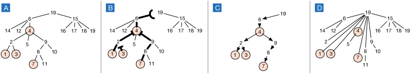
Figure 1: A: An example union-find tree with sample queries circled; B: Bolded edges are paths, together with their stopping points, that result from the traversal in Phase I; C: The traversal graph $R_{\cup}$ recorded as a result of Phase I; and D: The union-find tree after Phase II, which updates all traversed nodes to point to their roots.

5.1 Response Distributor

Consider a sequence $R_{\cup}=\langle(\textit{from}_{i},\textit{to}_{i})\rangle_{i=1}^{\lambda}$. We need a data structure RD such that after some preprocessing of $R_{\cup}$, can efficiently answer the query $\textit{RD}.\mbox{{allFrom}}(f)$ which returns a sequence containing all $\textit{to}_{i}$ where $\textit{from}_{i}=f$.

To meet the overall running time bound, the preprocessing step cannot take more than $O(\lambda)$ work and $O(\mathop{\mathrm{polylog}}(\lambda))$ depth. As far as we know, we cannot afford to generate, say, a sequence of sequences $RD$ where $RD[f]$ is a sequence containing all $\textit{to}_{i}$ such that $\textit{from}_{i}=f$. Instead, we propose a data structure with the following properties:

Lemma 9 (Response Distributor).

There is a data structure response distributor (RD) that from input $R_{\cup}=\langle(\textit{from}_{i},\textit{to}_{i})\rangle_{i=1}^{\lambda}$ can be constructed in $O(\lambda)$ work and $O(\mathop{\mathrm{polylog}}(n))$ depth. Each allFrom query can be answered in $O(\log\lambda)$ depth. Furthermore, if $\mathbb{F}$ is the set of unique $\textit{from}_{i}$ (i.e., $\mathbb{F}=\{\textit{from}_{i}\,:\,i=1,\dots,\lambda\}$), then

$$\mathop{\text{{E}}}\!\left[\sum_{f\in F}\textsf{Work}(\textit{RD}.\mbox{{allFrom}}(f))\right]=O(\lambda).$$

Proof.

Let $h$ be a hash function from the domain of $\textit{from}_{i}$’s (a subset of $[n]$) to $[\rho]$, where $\rho=3\lambda$. To construct an RD, we proceed as follows. Compute the hash for each $\textit{from}_{i}$ using $h(\cdot)$ and sort the ordered pairs $(\textit{from}_{i},\textit{to}_{i})$ by their hash values. Call this sorted array $A$. After sorting, we know that pairs with the same hash value are stored consecutively in $A$. Now create an array $o$ of length $\rho+1$ so that $o_{i}$ marks the beginning of pairs whose hash value is $i$. If none of them hash to $i$, $o_{i}=o_{i+1}$. These steps can be done using intSort and standard techniques in $O(\lambda)$ work and $O(\mathop{\mathrm{polylog}}(\lambda))$ depth because the hash values range within $O(\lambda)$.

To support $\mbox{{allFrom}}(f)$, we compute $\kappa=h(f)$ and look in $A$ between $o_{\kappa}$ and $o_{\kappa+1}-1$, selecting only pairs whose from matches $f$. This requires at most $O(\log|o_{\kappa+1}-o_{\kappa}|)=O(\log\lambda)$ depth. The more involved question is how much work is needed to support allFrom over all. To answer this, consider all the pairs in $R_{\cup}$ with $\textit{from}_{i}=f$. Let $n_{f}$ denote the number of such pairs. These $n_{f}$ pairs will be gone through by queries looking for $f$ and other entries that happen to hash to the same value as $f$ does. The exact number of times these pairs are gone through is $\beta_{f}:=\#\{s\in\mathbb{F}:h(f)=h(s)\}$. Hence, across all queries $f\in\mathbb{F}$, the total work is $\sum_{f\in\mathbb{F}}n_{f}\beta_{f}$. But $\mathop{\text{{E}}}\!\left[\beta_{f}\right]\leq 1+\frac{|\mathbb{F}|}{\rho}$, so

$$\sum_{f\in\mathbb{F}}\mathop{\text{{E}}}\!\left[n_{f}\beta_{f}\right]\leq\left(1+\tfrac{|\mathbb{F}|}{\rho}\right)\sum_{f\in\mathbb{F}}n_{f}\leq(1+\tfrac{\lambda}{3\lambda})\lambda\leq 2\lambda$$

because $|\mathbb{F}|\leq\lambda$ and $\sum_{f\in\mathbb{F}}n_{f}=\lambda$, completing the proof.

With this lemma, the cost of Bulk-Find can be stated as follows.

Lemma 10.

$\mbox{{Bulk-Find}}(U,S)$ does $O(|R_{\cup}|)$ work and has $O(\mathop{\mathrm{polylog}}(n))$ depth.

Proof.

The $R_{i}$’s, $F_{i}$’s, and $D_{i}$’s can be maintained directly as arrays. The roots and visited sets can be maintained as as bit flags on top of the vertices of $U$ as all we need are setting the bits (adding/removing elements) and reading their values (membership testing). There are two phases in this algorithm. In Phase I, the cost of adding $F_{i}$ to visited in iteration $i$ is bounded by $|R_{i}|$. Using standard parallel operations [11], the work of the other steps is clearly bounded by $|R_{i+1}|$, including mkFrontier because removeDup does work linear in the input, which is bounded by $|R_{i+1}|$. Thus, the work of Phase I is at most $O(\sum_{i}|R_{i}|)=O(|R_{\cup}|)$. In terms of depth, because the union-find tree has depth at most $O(\log n)$, the while loop can proceed for at most $O(\log n)$ times. Each iteration involves standard operations with depth at most $O(\log^{2}n)$, so the depth of Phase I is at most $O(\log^{3}n)$.

In Phase II, the dominant cost comes from expanding $D_{i}$ into $D_{i+1}$ by calling $\textit{RD}.\mbox{{allFrom}}$. By Lemma 9, across all iterations, the work caused by $\textit{RD}.\mbox{{allFrom}}$, run on each vertex once, is expected $O(|R_{\cup}|)$, and the depth is $O(\mathop{\mathrm{polylog}}(|R_{\cup}|))\leq O(\mathop{\mathrm{polylog}}(|R_{\cup}|))$. Overall, the algorithm requires $O(|R_{\cup}|)$ work and $O(\mathop{\mathrm{polylog}}(n))$ depth.

5.2 Bulk-Find’s Cost Equivalence to Serial find

In analyzing the work bound of the improved data structure, we will show that what Bulk-Find does is equivalent to some sequential execution of the standard find and requires the same amount of work, up to constants.

To gather intuition, we will manually derive such a sequence for the sample queries $S=\{1,3,4,7\}$ used in Figure 1. The query of $4$ went all the way to the root without merging with another flow. But the queries of $1$ and $7$ were stopped at $4$ and in this sense, depended upon the response from the query of $4$. By the same reasoning, because the query of $3$ merged with the query of $1$ (with $1$ proceeding on), the query of $3$ depended on the response from the query of $1$. Note that in this view, although the query of $3$ technically waited for the response at $2$, it was the query of $1$ that brought the response, so it depended on $1$. To derive a sequence execution, we need to respect the “depended on” relation: if $a$ depended on $b$, then $a$ will be invoked after $b$. As an example, one sequential execution order that respects these dependencies is $\mbox{{find}}(4),\mbox{{find}}(7),\mbox{{find}}(1),\mbox{{find}}(3)$.

We can check that by applying finds in this order, the paths traversed are exactly what the parallel execution does as $U.\mbox{{find}}{}$ performs full path compression.

We formalize this idea in the following lemma:

Lemma 11.

For a sequence of queries $S$ with which $\mbox{{Bulk-Find}}(U,S)$ is invoked, there is a sequence $S^{\prime}$ that is a permutation $S$ such that applying $U.\mbox{{find}}$ to $S^{\prime}$ serially in that order yields the same union-find forest as Bulk-Find’s and incurs the same traversal cost of $O(|R_{\cup}|)$, where $R_{\cup}$ is as defined in the Bulk-Find algorithm.

Proof.

For this analysis, we will associate every $(\textit{parent},\textit{child})\in R_{\cup}$ with a query $q\in S$. Logically, every query $q\in S$ starts a flow at $q$ ascending up the tree. If there are multiple flows reaching the same node, removeDup inside mkFrontier decides which flow to go on. From this view, for any nonroot node $u$ appearing in $R_{\cup}$, there is exactly one query flow from this node that proceeds up the tree. We will denote this flow by $\textsf{own}(u)$.

If a query flow is stopped partway (without reaching the corresponding root), the reason is either it merges in with another flow (via mkFrontier) or it recognizes another flow that visited where it is going before (via visited). For every query $q$ that is stopped partway, let $r(q)$ be the furthest point in the tree it has advanced to, i.e., $r(q)$ is the endpoint of the maximal path in $R_{\cup}$ for the query flow $q$.

In this set up, a query flow whose furthest point is $u$ will depend on the response from the query $\textsf{own}(u)$. Therefore, we form a dependency graph $G_{\textit{dep}}$ (“$u$ depends on $v$”) as follows. The vertices are all the vertices from $S$. For every query flow $q$ that is stopped partway, there is an arc $\textsf{own}(r(q))\to q$.

Let $S^{\prime}$ be a topologically-ordered sequence of $G_{\textit{dep}}$. Multiple copies of the same query vertex can simply be placed next to each other. If we apply $U.\mbox{{find}}{}$ serially on $S^{\prime}$, then all queries that a query vertex $q$ depends on in $G_{\textit{dep}}$ will have been called prior to $U.\mbox{{find}}(q)$. Because of full path compression, this means that $U.\mbox{{find}}(q)$ will follow $u\rightsquigarrow r(q)\to t$ ($r(q)\to t$ is one step), where $t$ is the root of the tree. Hence, every $U.\mbox{{find}}(q)$ traverses the same number of edges as $u\rightsquigarrow r(q)$ plus $1$. As every $R_{\cup}$ edge is part of a query flow, we conclude that the work of running $U.\mbox{{find}}$ on $S^{\prime}$ in that order is $O(|R_{\cup}|)$.

Finally, to obtain the bounds in Theorem 8, we modify Simple-Bulk-Query and Simple-Bulk-Update (in the relabeling step) to use Bulk-Find on all query pairs. The depth clearly remains $O(\mathop{\mathrm{polylog}}(n))$ per bulk operation. Aggregating the cost of Bulk-Find across calls from Bulk-Update and Bulk-Query, we know from Lemma 11 that there is a sequential order that has the same work. Therefore, the total work is bounded by $O((m+q)\alpha(m+q,n))$.

6 Implementation and Evaluation

This section discusses an implementation of the proposed data structure and its empirical performance.

6.1 Implementation

With an eye toward a simple implementation that delivers good practical performance, we set out to implement the simple bulk-parallel data structure from Section 4. The underlying union-find data structure $U$ maintains two arrays of length $n$—parent and sizes—one storing a parent pointer for each vertex, and the other tracking the sizes of the trees. The find and union operations follow a standard textbook implementation. On top of these operations, we implemented Simple-Bulk-Query and Simple-Bulk-Update as described earlier in the paper. We use standard sequence manipulation operations (e.g., filter, prefix sum, pack, remove duplicate) from the PBBS library [16]. There are two modifications that we made to improve practical performance of the implementation:

Path Compression: We wanted some benefits of path compression but without the full complexity of the work-efficient parallel algorithm from Section 5, to keep the code simple. We settled with the following pragmatic solution: The find operations inside Simple-Bulk-Query and Simple-Bulk-Update still run independently in parallel. But after finding the root, each operation traverses the tree one more time to update all the nodes on the path to point to the root. This leads to shorter paths for later bulk operations with clear performance benefits. However, for large bulk sizes, the approach may still perform significantly more work than the work-efficient solution because the path compression from a find operation may not benefit other find operations within the same minibatch.

Connected Components: The algorithm as described uses as a subroutine a linear-work parallel algorithm to find connected components. These linear work algorithms expect a graph representation that gives quick random access to the neighbors of a vertex. We found the processing cost to meet this requirement to be very high and instead implemented the algorithm for connectivity described in Blelloch et al. [3]. Although this has worse theoretical guarantees, it can work with a sequence of edges directly and delivers good real-world performance.

6.2 Experimental Setup

Environment: We performed experiments on an Amazon EC2 instance with $20$ cores (allowing for $40$ threads via hyperthreading) of $2.4$ GHz Intel Xeon E5-2676 v3 processors, running Linux 3.11.0-19 (Ubuntu 14.04.3). We believe this represents a baseline configuration of midrange workstations available in a modern cluster. All programs were compiled with Clang version 3.4 using the flag -O3. This version of Clang has the Intel Cilk runtime, which implements a work-stealing scheduler known to impose only a small overhead on both parallel and sequential code. We report wall-clock time measured using std::chrono::high_resolution_clock.

For robustness, we perform three trials and report the median running time. Although there is randomness involved in the connected component (CC) algorithm, we found no significant fluctuations in the running time across runs.

Datasets: Our study aims to study the behavior of the algorithm on a variety of graph streams. To this end, we use a collection of synthetic graph streams created using well-accepted generators. We include both power-law-type graphs and more regular graphs in the experiments. These are graphs commonly used in dynamic/streaming graph experiments (e.g., [13]). A summary of these datasets appear in Table 1.

Graph	#Vertices	#Edges	Notes
3Dgrid	$99.9$M	$300$M	3-d mesh
random	$100$M	$500$M	$5$ randomly-chosen neighbors per node
local5	$100$M	$500$M	small separators, avg. degree $5$
local16	$100$M	$1.6$B	small separators, avg. degree $16$
rMat5	$134$M	$500$M	power-law graph using rMat [4]
rMat16	$134$M	$1.6$B	a denser rMat graph

Table 1: Characteristics of the graph streams used in our experiments, showing for every dataset, the total number of nodes ($n$), the total number of edges ($m$), and a brief description.

The graph streams in our experiments differ substantially in how quickly they become connected. This input characteristic influences the data structure’s performance. In Figure 2, we show for each graph stream, the number of connected components at different points in the stream. The local16 graph becomes fully connected right around the midpoint of the stream. Both rMat5 and rMat16 continue to have tens of millions of components after consuming the whole stream. Note that in this figure, random and local5 are almost visually indistinguishable until the very end.

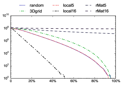
Figure 2: The numbers of connected components for each graph dataset at different percentages of the total graph stream processed.

Baseline: We directly compare our algorithms with union find (denoted UF), using both the union by size and a path compression variant, which has the optimal sequential running time. Most prior algorithms either focus on parallel graphs or streaming graphs, not parallel streaming graphs. We note that the algorithm of McColl et al. [13] that works in the parallel dynamic setting is not directly comparable to ours. Their algorithm focuses on supporting insertion and deletion of arbitrary edges, whereas ours is designed to take advantage of the insert-only setting.

6.3 Results

How does the bulk-parallel data structure perform on a multicore machine? To this end, we investigate the parallel overhead, speedup, and scalability trend.

Table 6.3 shows the timings for the baseline sequential implementation of union-find UF with and without path compression and the bulk-parallel implementation on a single thread for four different batch sizes, 500K, 1M, 5M, and 10M. To measure overhead, we first compare our implementation to union find without path compression: our implementation is between $1.01$x and $2.5$x slower except on local16, in which the bulk parallel achieves some speedups even on one thread. This is mainly because the number of connected components in local16 drops quickly to 1 as soon as midstream (Figure 2). With only 1 connected component, there is little work for bulk-parallel to be done after that. Compared to union find with path compression, our implementation, which does pragmatic path compression, shows nontrivial—but still acceptable—overhead, as to be expected because our solution does not fully benefit finds within the same minibatch.

Graph	UF	UF	Bulk-Parallel Using Batch Size
	(no p.c.)	(p.c.)	500K	1M	5M	10M
random	44.63	18.42	65.43	66.57	75.20	77.89
3Dgrid	30.26	14.37	61.10	62.00	71.74	75.07
local5	44.94	18.51	65.84	66.77	75.33	78.23
local16	154.40	46.12	114.34	108.92	114.80	117.55
rMat5	33.39	18.47	66.98	68.48	74.97	78.69
rMat16	81.74	35.29	83.27	76.64	76.03	77.62

Table 2: Running times (in seconds) on $1$ thread of the baseline union-find implementation UF with and without path compression (unaffected by the batch size) and the bulk-parallel data structure as the batch size is varied.

Table 6.3 shows the average throughputs (million edges/second) of Bulk-Update for different batch sizes. Here $T_{1}$ denotes the throughput on $1$ thread and $T_{20c}$ the throughput on $20$ cores (40 hyper-threads). We also show the speedup as measured by $T_{20c}/T_{1}$. We observe consistent speedup on all six datasets under all four batch sizes. Across all datasets, the general trend is that the larger the batch size, the higher was the speedup. This is to be expected, since a larger batch size means more work per core in processing each batch, and lesser overhead of synchronization.

Table 3: Average throughput (in million edges/second) and speedup of Bulk-Update for different batch sizes $b$, where $T_{1}$ is throughput on $1$ thread and $T_{20c}$ is the throughput on $20$ cores.

Figure 3 shows the average throughput (edges/sec) as the number of threads increases from 1 to $20c$, which represents 40 hyperthreads. Three different batch sizes were used for the experiments: 1M, 5M and 10M. The top chart represents the results on the random dataset, the middle chart on the local16 dataset and the bottom chart on the rMat16 dataset. In general, as the number of threads increases, the average throughput increases for all 3 datasets under different batch sizes. With a 10M batch size on 20 cores, we observe speedups between $8$–$11$x. On the rMat16 dataset (the bottom chart), the throughput starts to drop with batch size of 1M when the number of threads increases beyond 20. This is due to the relatively large number of connected components in the rMat16 dataset from the beginning towards the end of processing the entire dataset(see Figure 2). In this case, the work done per batch of input edges is relatively small, and a 1M batch size is too small for the rMat16 dataset to realize additional parallelization benefits beyond 20 threads.

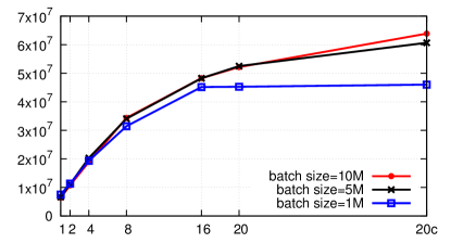
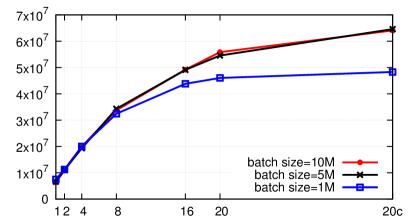
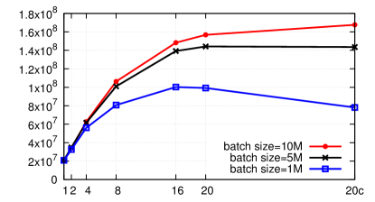
Figure 3: Average throughput (edges per second) as the number of threads is varied from 1 to $40$ (denoted by $20c$ as they run on 20 cores with hyperthreading). The graph streams shown are (top) random, (middle) local16, and (bottom) rMat16.

7 Conclusion

We presented a shared-memory parallel algorithm for incremental graph connectivity in the minibatch arrival model. Our algorithm has polylogarithmic parallel depth and its total work across all processors is of the same order as the work due to the best sequential algorithm for incremental graph connectivity. We also presented a simpler parallel algorithm that is easier to implement and has good practical performance.

This presents several natural open research questions. We list some of them here. (1) In case all edge updates are in a single minibatch, the total work of our algorithm is (in a theoretical sense), superlinear in the number of edges in the graph. Whereas, the optimal batch algorithm for graph connectivity, based on a depth-first search, has work linear in the number of edges. Is it possible to have an incremental algorithm whose work is linear in the case of very large batches, such as the above, and falls back to the union-find type algorithms for smaller minibatches? Note that for all practical purposes, the work of our algorithm is linear in the number of edges, due to very slow growth of the inverse Ackerman’s function. (2) Can these results on parallel algorithms be extended to the fully dynamic case when there are both edge arrivals as well as deletions?

References

- [1] Richard J. Anderson and Heather Woll. Wait-free parallel algorithms for the union-find problem. In Proceedings of the 23rd Annual ACM Symposium on Theory of Computing, May 5-8, 1991, New Orleans, Louisiana, USA, pages 370–380, 1991.
- [2] Jonathan Berry, Matthew Oster, Cynthia A. Phillips, Steven Plimpton, and Timothy M. Shead. Maintaining connected components for infinite graph streams. In Proc. 2nd International Workshop on Big Data, Streams and Heterogeneous Source Mining: Algorithms, Systems, Programming Models and Applications (BigMine), pages 95–102, 2013.
- [3] Guy E. Blelloch, Jeremy T. Fineman, Phillip B. Gibbons, and Julian Shun. Internally deterministic parallel algorithms can be fast. In Proceedings of the 17th ACM SIGPLAN Symposium on Principles and Practice of Parallel Programming, PPOPP 2012, New Orleans, LA, USA, February 25-29, 2012, pages 181–192, 2012.
- [4] Deepayan Chakrabarti, Yiping Zhan, and Christos Faloutsos. R-MAT: A recursive model for graph mining. In Proceedings of the Fourth SIAM International Conference on Data Mining, Lake Buena Vista, Florida, USA, April 22-24, 2004, pages 442–446, 2004.
- [5] Thomas H. Cormen, Charles E. Leiserson, Ronald L. Rivest, and Clifford Stein. Introduction to Algorithms (3. ed.). MIT Press, 2009.
- [6] Camil Demetrescu, Bruno Escoffier, Gabriel Moruz, and Andrea Ribichini. Adapting parallel algorithms to the W-stream model, with applications to graph problems. Theor. Comput. Sci., 411(44-46):3994–4004, 2010.
- [7] Camil Demetrescu, Irene Finocchi, and Andrea Ribichini. Trading off space for passes in graph streaming problems. ACM Transactions on Algorithms, 6(1), 2009.
- [8] Joan Feigenbaum, Sampath Kannan, Andrew McGregor, Siddharth Suri, and Jian Zhang. On graph problems in a semi-streaming model. Theor. Comput. Sci., 348(2-3):207–216, 2005.
- [9] Hillel Gazit. An optimal randomized parallel algorithm for finding connected components in a graph. SIAM J. Comput., 20(6):1046–1067, 1991.
- [10] IBM Corporation. Infosphere streams. http://www-03.ibm.com/software/products/en/infosphere-streams. Accessed Jan 2014.
- [11] Joseph JáJá. An Introduction to Parallel Algorithms. Addison-Wesley, 1992.
- [12] Bruce M. Kapron, Valerie King, and Ben Mountjoy. Dynamic graph connectivity in polylogarithmic worst case time. In Proceedings of the Twenty-Fourth Annual ACM-SIAM Symposium on Discrete Algorithms, SODA 2013, New Orleans, Louisiana, USA, January 6-8, 2013, pages 1131–1142, 2013.
- [13] Robert McColl, Oded Green, and David A. Bader. A new parallel algorithm for connected components in dynamic graphs. In 20th Annual International Conference on High Performance Computing, HiPC 2013, Bengaluru (Bangalore), Karnataka, India, December 18-21, 2013, pages 246–255, 2013.
- [14] Sanguthevar Rajasekaran and John H. Reif. Optimal and sublogarithmic time randomized parallel sorting algorithms. SIAM J. Comput., 18(3):594–607, 1989.
- [15] Raimund Seidel and Micha Sharir. Top-down analysis of path compression. SIAM J. Comput., 34(3):515–525, 2005.
- [16] Julian Shun, Guy E. Blelloch, Jeremy T. Fineman, Phillip B. Gibbons, Aapo Kyrola, Harsha Vardhan Simhadri, and Kanat Tangwongsan. Brief announcement: the problem based benchmark suite. In 24th ACM Symposium on Parallelism in Algorithms and Architectures, SPAA ’12, Pittsburgh, PA, USA, June 25-27, 2012, pages 68–70, 2012.
- [17] Julian Shun, Laxman Dhulipala, and Guy E. Blelloch. A simple and practical linear-work parallel algorithm for connectivity. In 26th ACM Symposium on Parallelism in Algorithms and Architectures, SPAA ’14, Prague, Czech Republic, pages 143–153, 2014.
- [18] Robert Endre Tarjan. Efficiency of a good but not linear set union algorithm. Journal of the ACM, 22(2):215–225, 1975.
- [19] M. Zaharia, T. Das, H. Li, T. Hunter, S. Shenker, and I. Stoica. Discretized streams: Fault-tolerant streaming computation at scale. In Proc. ACM Symposium on Operating Systems Principles (SOSP), pages 423–438, 2013.