Diphoton decay for a 750 GeV scalar boson in a $SU(6)\otimes U(1)_{X}$ model

Abstract

We propose a new $SU(6)\otimes U(1)_{X}$ GUT model free from anomalies, with a 750 GeV scalar candidate which can decay into two photons, compatible with the recent diphoton signal reported by ATLAS and CMS collaborations. This model gives masses to all fermions and may explain the 750GeV signal through one loop decays to $\gamma\gamma$ with charged vector and charged Higgs bosons, as well as up- and electron-like exotic particles that arise naturally from the condition of cancellation of anomalies of the $SU(6)\otimes U(1)_{X}$ group. We obtain, for different width approximations, allowed mass regions from 900 GeV to 3 TeV for the exotic up-like quark, in agreement with ATLAS and CMS collaborations data.

1 Introduction

Recently the ATLAS and CMS collaborations reported a diphoton signal excess with invariant mass of 750 GeV [1, 2] which has been the subject of many interpretations in the literature using different extensions of the standard model (SM) [3, 4, 5, 6, 7, 8, 9, 10, 11]. In this work, we consider the $SU(6)\otimes U(1)_{X}$ extension proposed in [13] in the framework of the flipped $SU(6)$ models [12] as a feasible model that may explain the diphoton excess. These kind of flipped models have very interesting features. First, by requiring a high breaking scale ($\sim 10^{17}$ GeV) for the flipped $SU(6)$ and its $SU(5)$ subgroup [14] the proton decay problem can be avoid. Second, they are able to solve the doublet-triplet splitting problem through the pseudo-Goldstone mechanism as in $SU(6)$ [15, 16] and $[SU(3)]^{3}$ [17]. Also, they provide unification of gauge couplings as in the flipped $SU(5)$ model [18, 19]. Finally, these models may develop see-saw masses compatible with the phenomenological active neutrinos [20, 21] if one singlet heavy state is introduced.

The $SU(6)\otimes U(1)_{X}$ extension considered here contains the $SU(3)_{C}\otimes SU(3)_{L}\otimes U(1)_{X}$ model (hereafter 331 model) [22, 23, 24, 25] as a subgroup that allow us address the observed diphoton excess through new exotic charged Higgs bosons into the loop at the TeV scale. In the flipped model, the $U(1)_{X}$ symmetry changes the exotic down type quark (charge $-1/3$) by an up type quark (charge $2/3$) in the multiplets, which increases the coupling with photons and gluons into the loop, resulting in a significantly enhanced $pp\rightarrow\gamma\gamma$ cross section, compatible with the reported data.

The 331 model can be embedded into the grand unified group $SU(6)\otimes U(1)_{X}$ with the following spontaneous symmetry breaking (SSB) chain:

$$SU(6)\otimes U(1)_{X}\overset{{\mathbf{\Phi}}}{\xrightarrow{\hskip 14.22636pt}}SU(3)_{C}\otimes SU(3)_{L}\otimes U(1)_{X}\overset{H_{1},H_{S}}{\xrightarrow{\hskip 28.45274pt}}$$ (1)

$$SU(3)_{C}\otimes SU(2)_{L}\otimes U(1)_{Y}\overset{H_{2},H_{3},H_{S}}{\xrightarrow{\hskip 42.67912pt}}SU(3)_{C}\otimes U(1)_{Q}$$

which are mediated by the five Higgs fields $\Phi$, $H_{1}$, $H_{2}$ , $H_{3}$ and $H_{S}$ in the $\mathbf{35}$, $\bar{\mathbf{6}}$, $\bar{\mathbf{6}}$ ,$\bar{\mathbf{15}}$ and $\bar{\mathbf{15}}$ representations, respectively. From the mixing of the real components of the fields $H_{1}$ and $H_{S}$ we will obtain two real scalar fields, our candidate for the 750 GeV signal ($\xi$), and the other at the TeV scale ($\xi^{\prime}$).

This paper is organized as follows. In section 2, we show the particle content of a $SU(6)\otimes U(1)_{X}$ model as an anomaly free theory which contains the 331, 321 and 31 subgroups and their SSB scheme. We describe the Yukawa Lagrangian showing that four Higgs fields are sufficient to give masses to all fermions. We also show the most general Higgs potential terms compatible with the symmetries and identify the relevant quartic couplings that will induce the process $pp\rightarrow\xi\rightarrow\gamma\gamma$. Section 3 is devoted to explore allowed regions consistent with the reported cross section of the 750 GeV signal. Finally, in section 4, we summarize our conclusions.

2 $SU(6)\otimes U(1)_{X}$ model

$SU(6)\otimes U(1)_{X}$ strong-electroweak models provide us a new framework which contains 331 and SM models for one family of fermions as effective low energy field theories. In order to include the three families we consider replicas of the first family as in the SM. Below, we describe some remarkable properties of these models.

• The cancellation of the $[SU(6)]^{3}$, $[SU(6)]^{2}U(1)_{X}$, $[\mathrm{Grav}]^{2}U(1)_{X}$ and $[U(1)_{X}]^{3}$ chiral anomaly equations, shown in reference [13], provide us a set of multiplets with non-trivial $U(1)_{X}$ charges which are family independent. We require two sextets $\mathbf{\bar{6}}$, one antisymmetric $\mathbf{15}$ multiplet and three singlets with charges $X_{\mathbf{\bar{6}}}=-2/3$, $X_{\mathbf{15}}=1/3$ and $X_{\mathbf{1}}=1$, respectively.

• The symmetry breaking $SU(6)\rightarrow SU(3)_{C}\otimes SU(3)_{L}\otimes U(1)_{Y^{\prime}}$ gives us the following branching rules:

  $$\bar{\mathbf{6}} =(\bar{\mathbf{3}}_{C}\otimes\mathbf{1}_{L})_{1/3}\oplus(\mathbf{1}_{C}\otimes\mathbf{3}_{L})_{-1/3},$$ (2)

  $$\mathbf{15} =(\bar{\mathbf{3}}_{C}\otimes\mathbf{1}_{L})_{2/3}\oplus(\mathbf{1}_{L}\otimes\mathbf{3}_{L})_{-2/3}\oplus(\mathbf{3}_{C}\otimes\bar{\mathbf{3}}_{L})_{0},$$ (3)

  where $(\mathbf{n}\otimes\mathbf{m})_{Y^{\prime}}$ are tensorial products of $\mathbf{n}$ $SU(3)_{C}$ multiplet with $\mathbf{m}$ $SU(3)_{L}$ multiplets and $Y^{\prime}$ corresponds to the $U(1)_{Y^{\prime}}$ quantum number normalized as $2Y^{\prime}/\sqrt{3}$, where:

  $$Y^{\prime}=\frac{1}{2\sqrt{3}}\;\mathrm{diag}\left(\begin{array}[]{cccccc}+1&+1&+1&-1&-1&-1\end{array}\right).$$ (4)

  This gives us the following multiplets for the first family:

  $$\psi_{L}=\left(\begin{array}[]{c}u^{c}\\ u^{c}\\ u^{c}\\ \nu_{e}\\ e^{-}\\ E^{-}\end{array}\right)_{L}\qquad\chi_{L}=\left(\begin{array}[]{c}U^{c}\\ U^{c}\\ U^{c}\\ N_{E}\\ E_{1}^{-}\\ E_{2}^{-}\end{array}\right)_{L}\qquad\Psi_{L}=\left(\begin{array}[]{cccccc}0&d^{c}&-d^{c}&d&u&U\\ -d^{c}&0&d^{c}&d&u&U\\ d^{c}&-d^{c}&0&d&u&U\\ -d&-d&-d&0&\nu_{e1}^{c}&-N_{E1}^{c}\\ -u&-u&-u&-\nu_{e}^{c}&0&E_{1}^{+}\\ -U&-U&-U&N_{E}^{c}&-E_{1}^{+}&0\end{array}\right)_{L}$$ (5)

  $$\mathbf{1}:\qquad e_{L}^{+},\qquad E_{L}^{+},\qquad E_{2L}^{+},\qquad\nu_{SL}$$ (6)

  where $U$ is a new up-like quark, $E^{-}$, $E_{1}^{-}$ and $E_{2}^{-}$ are new exotic charged leptons and $\nu_{e1R}$, $N_{EL}$ and $N_{ER1}$ are new neutrinos. In order to obtain fermion mass hierarchies among families, discrete symmetries can be introduced to obtain suitable mass matrix ansatz. The additional sterile neutrino $\nu_{S}$ with $X_{S}=0$ is necessary to produce see-saw mechanisms between neutrinos [26, 27, 28].

• The covariant derivatives for each type of multiplets are defined as follows:

  $$D_{\mu}\psi_{a} = \partial_{\mu}\psi_{a}+i\left(g_{6}A_{\mu}^{\alpha}(T_{\alpha})_{\;a}^{b}\right)\psi_{b}+ig_{X}\left(X_{\bar{\mathbf{6}}}\right)_{\;a}^{b}X^{\prime\mu}\psi_{b},$$ (7)

  $$D_{\mu}\Psi^{ab} = \partial_{\mu}\Psi^{ab}-i\left(g_{6}A_{\mu}^{\alpha}(T_{\alpha})_{\;cd}^{ab}\right)\Psi^{cd}-ig_{X}\left(X_{\mathbf{15}}\right)_{\;cd}^{ab}X^{\prime\mu}\Psi^{cd},$$ (8)

  where Latin indices run from 1 to 6, while Greek indices run from 1 to 35. The$\mathbf{15}$ generators are given by $(T_{\alpha})_{\;cd}^{ab}=(T_{\alpha})_{\;c}^{a}\delta_{\;d}^{b}+\delta_{\;c}^{a}(T_{\alpha})_{\;d}^{b}$.

• Gauge bosons are described by the $\mathbf{35}=\bar{\mathbf{35}}$ adjoint representation which obey the branching rule

  $$\begin{aligned} \mathbf{35}=(\mathbf{8}\otimes\mathbf{1})_{0}\oplus(\mathbf{1}\otimes\mathbf{8})_{0}\oplus(\mathbf{3}\otimes\bar{\mathbf{3}})_{2/3}\oplus(\bar{\mathbf{3}}\otimes\mathbf{3})_{-2/3}\oplus(\mathbf{1}\otimes\mathbf{1})_{0}\end{aligned},$$ (9)

  where $(\mathbf{8}\otimes\mathbf{1})_{0}$ are identified as QCD gluons; $(\mathbf{1}\otimes\mathbf{8})_{0}$ are electro-weak gauge bosons which contains $W^{\pm}_{\mu}$, $W^{\pm}_{3\mu}$, $W^{0}_{3\mu}$, $\overline{W}^{0}_{3\mu}$, $A^{3}_{\mu}$ and $A^{8}_{\mu}$ bosons; $(\mathbf{1}\otimes\mathbf{1})_{0}$ is a neutral boson $B_{Y^{\prime}{\mu}}$ from the $U(1)_{Y^{\prime}}$ symmetry, and $(\mathbf{3}\otimes\bar{\mathbf{3}})_{2/3}$ and $(\bar{\mathbf{3}}\otimes\mathbf{3})_{-2/3}$ are new leptoquark bosons: $X_{\mu}$ with electric charge $2/3$, and $Y_{1{\mu}}$ and $Y_{{\mu}2}$ with electric charge $-1/3$, which induces quark-lepton interchange processes. Their corresponding multiplet is:

  $$\mathbf{A}=\frac{1}{\sqrt{2}}\left(\begin{array}[]{cccccc}G_{\;\;1}^{1}&G_{\;\;2}^{1}&G_{\;\;3}^{1}&X^{1c}&Y_{1}^{1c}&Y_{2}^{1c}\\ G_{\;\;1}^{2}&G_{\;\;2}^{2}&G_{\;\;3}^{2}&X^{2c}&Y_{1}^{2c}&Y_{2}^{2c}\\ G_{\;\;1}^{3}&G_{\;\;2}^{3}&G_{\;\;3}^{3}&X^{3c}&Y_{1}^{3c}&Y_{2}^{3c}\\ X^{1}&X^{2}&X^{3}&D_{1}&W^{+}&W_{3}^{+}\\ Y_{1}^{1}&Y_{1}^{2}&Y_{1}^{3}&W^{-}&D_{2}&W_{3}^{0}\\ Y_{2}^{1}&Y_{2}^{2}&Y_{2}^{3}&W_{3}^{-}&\overline{W}_{3}^{0}&D_{3}\end{array}\right)$$ (10)

  where $G_{\;\;1}^{1}+G_{\;\;2}^{2}+G_{\;\;3}^{3}=0$. $D_{1}=A^{3}/\sqrt{2}+A^{8}/\sqrt{6}$, $D_{2}=-A^{3}/\sqrt{2}+A^{8}/\sqrt{6}$ and $D_{3}=-\sqrt{2}A^{8}/\sqrt{3}$ are the diagonal $SU(3)_{L}$ gauge fields. In addition, there is a new electrically neutral vector boson $X_{\mu}$ from $U(1)_{X}$ symmetry. In total, the $SU(6)\otimes U(1)_{X}$ group has 36 gauge bosons: eight gluons, eight electroweak bosons, eighteen leptoquark bosons and two electrically neutral bosons.

• Electric charge are constructed using all diagonal generators of $SU(6)\otimes U(1)_{X}$:

  $${Q}=aT_{3}+\frac{2b}{\sqrt{3}}T_{8}+\frac{2c}{\sqrt{6}}T_{15}+\frac{2d}{\sqrt{10}}T_{24}+\frac{2e}{\sqrt{15}}T_{35}+XI_{6},$$ (11)

  where the $a,b,c,d,e$ and $f$ constants are fixed such that the electric charge match with each charge from the multiplets. We find

  $${Q}=T_{3L}-\frac{1}{2\sqrt{6}}T_{15}-\frac{1}{2\sqrt{10}}T_{24}+\frac{2}{\sqrt{15}}T_{35}+XI_{6}=T_{3L}+\frac{Y}{2},$$ (12)

  where $Y$ is the usual hypercharge operator of the SM.

• The fermions contained in the model have the charges listed in Table 1.

  Left-handed
  	$T_{3L}$	$X$	$Y$	$Q$
  $u$	$+1/2$	$+1/3$	$+1/3$	$+2/3$
  $d$	$-1/2$	$+1/3$	$+1/3$	$-1/3$
  $U$	$0$	$+1/3$	$+4/3$	$+2/3$
  $\nu_{e}$	$+1/2$	$-2/3$	$-1$	$0$
  $e^{-}$	$-1/2$	$-2/3$	$-1$	$-1$
  $N_{E}$	$+1/2$	$-2/3$	$-1$	$0$
  $E_{1}^{-}$	$-1/2$	$-2/3$	$-1$	$-1$
  $E^{-}$	$0$	$-2/3$	$-2$	$-1$
  $E_{2}^{-}$	$0$	$-2/3$	$-2$	$-1$

      Right-handed $T_{3L}$ $X$ $Y$ $Q$ $u$ $0$ $+2/3$ $+4/3$ $+2/3$ $d$ $0$ $+1/3$ $-2/3$ $-1/3$ $U$ $0$ $+2/3$ $+4/3$ $+2/3$ $\nu_{e1}$ $0$ $-1/3$ $0$ $0$ $e^{-}$ $0$ $-1$ $-2$ $-1$ $N_{E1}$ $+1/2$ $-1/3$ $-1$ $0$ $E_{1}^{-}$ $-1/2$ $-1/3$ $-1$ $-1$ $E^{-}$ $0$ $-1$ $-2$ $-1$ $E_{2}^{-}$ $0$ $-1$ $-2$ $-1$

  Table 1: Quantum numbers for the fermionic sector of the model.

• The scalar sector is introduced to obtain the correct SSB chain. The two last symmetry breakings are fulfilled using two Higgs fields represented by sextets $\bar{\mathbf{6}}$ with $X_{H_{1},H_{2}}=1/3$. The directions of their VEV, $V_{1}$ and $v_{2}$, are selected to obtain electrically neutral vacua. In addition, $V_{1}$ is at the TeV scale while $v_{2}$ is at the electroweak scale. Two additional Higgs fields represented by $\mathbf{\bar{15}}$ multiplets with $X_{H_{3}}=-2/3$ and $X_{H_{S}}=1/3$ are introduced to give masses to down quarks and neutrinos, respectively.

  The first SSB needs a Higgs field from $\mathbf{35}$ adjoint representation with the following VEV:

  $$\left\langle\Phi\right\rangle_{0}=\mathcal{V}_{\mathrm{GUT}}\;\mathrm{diag}\left(\begin{array}[]{cccccc}+1&+1&+1&-1&-1&-1\end{array}\right),$$ (13)

  where $\mathcal{V}_{\mathrm{GUT}}\sim 10^{17}$ GeV breaks the gauge symmetry to $SU(3)_{C}\otimes SU(3)_{L}\otimes U(1)_{Y^{\prime}}$ providing masses to the leptoquark bosons. For the second and third SSBs, we define the following Higgs scalar multiplets:

  $$H_{1}=\left(\begin{array}[]{c}\phi_{1}^{1/3}\\ \phi_{1}^{1/3}\\ \phi_{1}^{1/3}\\ \varphi_{1}^{+}\\ \varphi_{1}^{0}\\ \frac{\xi_{1}+V_{1}+i\zeta_{1}}{\sqrt{2}}\end{array}\right),\qquad H_{2}=\left(\begin{array}[]{c}\phi_{2}^{1/3}\\ \phi_{2}^{1/3}\\ \phi_{2}^{1/3}\\ \varphi_{2}^{+}\\ \frac{h_{2}+v_{2}+i\eta_{2}}{\sqrt{2}}\\ \varphi_{2}^{0}\end{array}\right)$$ (14)

  $$H_{3}=\left(\begin{array}[]{cccccc}0&\phi_{3}^{2/3}&-\phi_{3}^{2/3}&\phi_{3}^{4/3}&\phi_{31}^{1/3}&\phi_{32}^{1/3}\\ -\phi_{3}^{2/3}&0&\phi_{3}^{2/3}&\phi_{3}^{4/3}&\phi_{31}^{1/3}&\phi_{32}^{1/3}\\ \phi_{3}^{2/3}&-\phi_{3}^{2/3}&0&\phi_{3}^{4/3}&\phi_{31}^{1/3}&\phi_{32}^{1/3}\\ -\phi_{3}^{4/3}&-\phi_{3}^{4/3}&-\phi_{3}^{4/3}&0&\phi_{3}^{+}&-\varphi_{3}^{+}\\ -\phi_{31}^{1/3}&-\phi_{31}^{1/3}&-\phi_{31}^{1/3}&-\phi_{3}^{+}&0&\frac{h_{3}+v_{3}+i\eta_{3}}{\sqrt{2}}\\ -\phi_{32}^{1/3}&-\phi_{32}^{1/3}&-\phi_{32}^{1/3}&\varphi_{3}^{+}&-\frac{h_{3}+v_{3}+i\eta_{3}}{\sqrt{2}}&0\end{array}\right),$$ (15)

  $$H_{S}=\left(\begin{array}[]{cccccc}0&\phi_{S}^{-1/3}&-\phi_{S}^{-1/3}&\phi_{S}^{1/3}&\phi_{S1}^{-2/3}&\phi_{S2}^{-2/3}\\ -\phi_{S}^{-1/3}&0&\phi_{S}^{-1/3}&\phi_{S}^{1/3}&\phi_{S1}^{-2/3}&\phi_{S2}^{-2/3}\\ \phi_{S}^{-1/3}&-\phi_{S}^{-1/3}&0&\phi_{S}^{1/3}&\phi_{S1}^{-2/3}&\phi_{S2}^{-2/3}\\ -\phi_{S}^{1/3}&-\phi_{3}^{4/3}&-\phi_{3}^{4/3}&0&\frac{\xi_{S}+V_{S}-i\zeta_{S}}{\sqrt{2}}&-\frac{h_{S}+v_{S}-i\eta_{S}}{\sqrt{2}}\\ -\phi_{S1}^{-2/3}&-\phi_{S1}^{-2/3}&-\phi_{S1}^{-2/3}&-\frac{\xi_{S}+V_{S}-i\zeta_{S}}{\sqrt{2}}&0&\varphi_{S}^{+}\\ -\phi_{S2}^{-2/3}&-\phi_{S2}^{-2/3}&-\phi_{S2}^{-2/3}&\frac{h_{S}+v_{S}-i\eta_{S}}{\sqrt{2}}&-\varphi_{S}^{+}&0\end{array}\right),$$ (16)

  where $V_{1},V_{S}\gg v_{2},v_{3},v_{S}\sim 246\mathrm{GeV}$. In this way, the SSB chain is given by Eq.(1).

• Vector boson masses: there are two electroweak SSBs in the low-energy $SU(3)_{L}\otimes U(1)_{X}$ model, the first $V$ at TeV and the second at $v$ GeV scale. After the TeV SSB $SU(3)_{L}\otimes U(1)_{X}\rightarrow SU(2)_{L}\otimes U(1)_{Y}$ the gauge bosons $A_{\mu}^{8}$ and $X_{\mu}$ mix them together into the weak hypercharge boson $B_{\mu}$ and a new massive electrically neutral gauge boson $Z_{X\mu}$ trough the following mixing matrix with the mixing angle $\tan\theta_{X}=-\sqrt{3}{g}/{g_{X}}$,

  $$\left(\begin{array}[]{c}B\\ Z_{X}\end{array}\right)=\left(\begin{array}[]{cc}\cos\theta_{X}&-\sin\theta_{X}\\ \sin\theta_{X}&\cos\theta_{X}\end{array}\right)\left(\begin{array}[]{c}A^{8}\\ -X\end{array}\right).$$ (17)

  The new gauge coupling constant is the electroweak hypercharge $g^{\prime}=g_{X}\sin\theta_{X}=-\sqrt{3}g\cos\theta_{X}$. The gauge bosons $W_{3\mu}^{\pm}$, $W_{3\mu}^{0}$ and $\overline{W}_{3\mu}^{0}$ acquire the same mass $M_{W_{3}}$ which is related to $M_{Z_{X}}$ by $\sin\theta_{W}$ in the following way

  $$M_{W_{3}}=\frac{gV}{2}\qquad,\qquad M_{Z_{X}}=\frac{gV}{\sqrt{3}\sin\theta_{X}}=\frac{2}{\sqrt{3}}\frac{M_{W_{3}}}{\sin\theta_{X}}$$ (18)

  where $V^{2}=V_{1}^{2}+2V_{S}^{2}$. In addition, the $\xi$ gauge couplings are given by

  $$\begin{split}\mathcal{L_{\xi VV}}&=\frac{\mathit{V}g^{2}}{3\sin^{2}\theta_{X}}\xi{Z_{X\mu}Z_{X}^{\mu}}+\frac{\mathit{V}{{\mathit{g}}^{2}}}{2}\xi\mathit{W_{3\mu}^{-}}\mathit{W_{3}^{+\mu}}+\frac{\mathit{V}{{\mathit{g}}^{2}}}{2}\xi\mathit{W_{3\mu}^{0}}\mathit{\overline{W}_{3}^{0\mu}}\\ &=\frac{M_{Z_{1}}^{2}}{V}\xi{Z_{X\mu}Z_{X}^{\mu}}+2\frac{M_{W_{3}}^{2}}{V}\xi\mathit{W_{3\mu}^{-}}\mathit{W_{3}^{+\mu}}+2\frac{M_{W_{3}}^{2}}{V}\xi\mathit{W_{3\mu}^{0}}\mathit{\overline{W}_{3}^{0\mu}}.\end{split}$$ (19)

  Here $\xi$ does not couple to $B_{\mu}$ because $M_{B}=0$. Secondly, for the GeV SSB $SU(2)_{L}\otimes U(1)_{Y}\rightarrow U(1)_{Q}$ will bring the well-known gauge boson mixing through the Weinberg angle $\tan\theta_{W}={g^{\prime}}/{g}$

  $$\left(\begin{array}[]{c}Z_{W}\\ A\end{array}\right)=\left(\begin{array}[]{cc}\cos\theta_{W}&-\sin\theta_{W}\\ \sin\theta_{W}&\cos\theta_{W}\end{array}\right)\left(\begin{array}[]{c}A^{3}\\ B\end{array}\right).$$ (20)

  The new gauge coupling constant is the electromagnetic charge $e=g_{2}\sin\theta_{W}=g_{Y}\cos\theta_{W}$ and the new gauge boson masses are

  $$M_{W_{3}^{+}}=\frac{g}{2}\sqrt{V^{2}+v^{2}},\qquad M_{W_{3}^{0}}=\frac{gV}{2},\qquad M_{W^{+}}=\frac{gv}{2}$$ (21)

  where $v^{2}=v_{2}^{2}+2v_{3}^{2}+2v_{S}^{2}=(246\mathrm{\,GeV})^{2}$. In addition, $Z_{W\mu}$ and $Z_{X\mu}$ acquire the following masses

  $$M_{Z_{W}}=\frac{gv}{2\cos\theta_{W}}=\frac{M_{W}}{\cos\theta_{W}},\qquad M_{Z_{X}}=\frac{2}{\sqrt{3}}\frac{M_{W_{3}}}{\sin\theta_{X}}.$$ (22)

  There is an additional gauge boson mixing between the two neutral $Z_{W}$ and $Z_{X}$ through the mixing angle $\tan\theta_{Z}\propto{v^{2}}/{V^{2}}$,

  $$\left(\begin{array}[]{c}Z\\ Z^{\prime}\end{array}\right)=\left(\begin{array}[]{cc}\cos\theta_{Z}&\sin\theta_{Z}\\ -\sin\theta_{Z}&\cos\theta_{Z}\end{array}\right)\left(\begin{array}[]{c}Z_{W}\\ Z_{X}\end{array}\right)$$ (23)

  obtaining the physical gauge boson masses $Z$ and $Z^{\prime}$,

  $$M_{Z}\approx M_{Z_{W}}\sqrt{1+\mathcal{O}\left(\frac{v^{2}}{V^{2}}\right)},\qquad M_{Z^{\prime}}\approx M_{Z_{X}}\sqrt{1-\mathcal{O}\left(\frac{v^{2}}{V^{2}}\right)}$$ (24)

2.1 Yukawa Lagrangian

The Yukawa Lagrangian that describes interactions between the Higgs and the fermion sector is the following

$$-\mathcal{L}_{\mathrm{Yukawa}}= \sum_{i=1,2}(\psi_{La}^{\mathrm{T}}\hat{C}h_{\psi i}\Psi_{L}^{ab}H_{ib}+\psi_{La}^{\mathrm{T}}\hat{C}h_{\psi ei}H_{i}^{a}e_{L}^{+}+\psi_{La}^{\mathrm{T}}\hat{C}h_{\psi Ei}H_{i}^{a}E_{L}^{+}+\psi_{La}^{\mathrm{T}}\hat{C}h_{\psi E_{2}i}H_{i}^{a}E_{2L}^{+}$$

$$+\;\chi_{La}^{\mathrm{T}}\hat{C}h_{\chi i}\Psi_{L}^{ab}H_{ib}+\chi_{La}^{\mathrm{T}}\hat{C}h_{\chi ei}H_{i}^{a}e_{L}^{+}+\chi_{La}^{\mathrm{T}}\hat{C}h_{\chi Ei}H_{i}^{a}E_{L}^{+}+\chi_{La}^{\mathrm{T}}\hat{C}h_{\chi E_{2}i}H_{i}^{a}E_{2L}^{+})+$$

$$+\;h_{3}\epsilon_{abcdef}\Psi_{L}^{\mathrm{T}ab}\hat{C}\Psi_{L}^{dc}H_{3}^{ef}+{\Psi_{L}^{\mathrm{T}}}^{ab}\hat{C}h_{S}{H_{S}}_{ab}\nu_{SL}+\nu_{SL}^{T}\hat{C}M_{S}\nu_{SL}+h.c,$$ (25)

where $a,\cdots,f=1,\cdots,6$. The terms $\psi_{La}^{\mathrm{T}}\hat{C}h_{\psi i}\Psi_{L}^{ab}H_{ib}$ and $\chi_{La}^{\mathrm{T}}\hat{C}h_{\chi i}\Psi_{L}^{ab}H_{ib}$ give masses to up quarks and leptons at the order of $\left\langle H_{i}\right\rangle$ and with Yukawa coupling constants $h_{\psi i}$ and $h_{\chi i}$. Terms containing couplings with singlet leptons, as for example $\psi_{La}^{\mathrm{T}}\hat{C}h_{\psi ei}H_{i}^{a}e_{L}^{+}$, give masses to $e_{L}^{+}$, $E_{L}^{+}$ and $E_{2L}^{+}$ with coupling constants $h_{\psi ei}$, $h_{\psi Ei}$ and $h_{\psi E_{2}i}$, respectively. The term that contains couplings with the scalar fields $H_{3}$, gives masses to down quarks with coupling constant $h_{3}$. The last two terms in Eq. (25) induce see-saw neutrino masses [29, 30, 31, 32], where $\nu_{SL}$ is a Majorana neutrino of mass $M_{S}$ which is fixed to give a light neutrino $\nu_{e}$, with mass at the order of eV.

First, for up quarks, we obtain the following non-diagonal mass matrix,

$$M_{uU}^{0}=\left(\begin{array}[]{cc}h_{\psi 2}v_{2}&h_{\psi 1}V_{1}\\ h_{\chi 2}v_{2}&h_{\chi 1}V_{1}\end{array}\right)$$ (26)

By diagonalizing the symmetric matrix $\left(M_{uU}^{0}\right)^{\mathrm{T}}M_{uU}^{0}$, we obtain the following masses

$$m_{U} \approx \sqrt{\frac{h_{\chi 1}^{2}+h_{\psi 1}^{2}}{2}}V_{1},$$

$$m_{u} \approx \frac{h_{\chi 1}h_{\psi 2}-h_{\psi 1}h_{\chi 2}}{\sqrt{h_{\chi 1}^{2}+h_{\psi 1}^{2}}}v_{2}.$$ (27)

Charged leptons acquire masses through the following mass matrix in the $(e^{-},E^{-},E_{1}^{-},E_{2}^{-})$ basis,

$$M_{E}=\left(\begin{array}[]{cccc}h_{\psi e2}v_{2}&h_{\psi E2}v_{2}&h_{\psi 1}V_{1}&h_{\psi E_{2}2}v_{2}\\ h_{\psi e1}V_{1}&h_{\psi E1}V_{1}&-h_{\psi 2}v_{2}&h_{\psi E_{2}1}V_{1}\\ h_{\chi e2}v_{2}&h_{\chi E2}v_{2}&h_{\chi 1}V_{1}&h_{\chi E_{2}2}v_{2}\\ h_{\chi e1}V_{1}&h_{\chi E1}V_{1}&-h_{\chi 2}v_{2}&h_{\chi E_{2}1}V_{1}\end{array}\right),$$ (28)

while neutrinos acquire masses through the following mass matrix in the $(\nu_{e},\nu_{e1}^{c},N_{E},N_{E1}^{c},\nu_{S})$ basis,

$$M_{N}=\left(\begin{array}[]{ccccc}0&h_{\psi 2}v_{2}&0&-h_{\psi 1}V_{1}&0\\ h_{\psi 2}v_{2}&0&h_{\chi 2}v_{2}&0&h_{S}V_{S}\\ 0&h_{\chi 2}v_{2}&0&-h_{\chi 1}V_{1}&0\\ -h_{\psi 1}V_{1}&0&-h_{\chi 1}V_{1}&0&h_{S}v_{S}\\ 0&h_{S}V_{S}&0&h_{S}v_{S}&M_{S}\end{array}\right).$$ (29)

Finally, the down quark acquire mass proportional to $\langle H_{3}\rangle=v_{3}$,

$$m_{d}=\sqrt{2}h_{3}v_{3}.$$ (30)

2.2 Higgs potential

The interactions between the four Higgs bosons are described by the following scalar potential,

$$V(H_{1},H_{2},H_{3},H_{S},\Phi)= -\mu_{1}^{2}H_{1}^{\dagger}H_{1}-\mu_{2}^{2}H_{2}^{\dagger}H_{2}-\mu_{3}^{2}\mathrm{Tr}(H_{3}^{\dagger}H_{3})-\mu_{S}^{2}\mathrm{Tr}(H_{S}^{\dagger}H_{S})^{2}-\mu_{\Phi}^{2}\mathrm{Tr}(\Phi)^{2}+$$

$$\lambda_{1}(H_{1}^{\dagger}H_{1})^{2}+\lambda_{2}(H_{2}^{\dagger}H_{2})^{2}+\lambda{}_{3}\mathrm{Tr}(H_{3})^{4}+\lambda^{\prime}_{3}(\mathrm{Tr}(H_{3})^{2})^{2}+$$

$$\lambda{}_{S}\mathrm{Tr}(H_{S})^{4}+\lambda^{\prime}_{S}(\mathrm{Tr}(H_{S})^{2})^{2}+\lambda{}_{\Phi}\mathrm{Tr}(\Phi)^{4}+\lambda^{\prime}_{\Phi}(\mathrm{Tr}(\Phi)^{2})^{2}+$$

$$\lambda_{12}(H_{1}^{\dagger}H_{1})(H_{2}^{\dagger}H_{2})+\lambda_{1S}(H_{1}^{\dagger}H_{1})\mathrm{Tr}(H_{S}^{\dagger}H_{S})^{2}+\lambda^{\prime}_{1S}(H_{1}^{\dagger}(H_{S})^{2}H_{1})+$$

$$\lambda_{13}(H_{1}^{\dagger}H_{1})\mathrm{Tr}(H_{3})^{2}+\lambda^{\prime}_{13}(H_{1}^{\dagger}(H_{3})^{2}H_{1})+\lambda_{2S}(H_{2}^{\dagger}H_{2})\mathrm{Tr}(H_{S}^{\dagger}H_{S})^{2}+$$

$$\lambda^{\prime}_{2S}(H_{2}^{\dagger}(H_{S})^{2}H_{2})+\lambda_{23}(H_{2}^{\dagger}H_{2})\mathrm{Tr}(H_{3})^{2}+\lambda^{\prime}_{23}(H_{2}^{\dagger}(H_{3})^{2}H_{2})+$$ (31)

$$\lambda_{3S}(\mathrm{Tr}H_{3}^{2})(\mathrm{Tr}H_{S}^{2})+\lambda^{\prime}_{3S}\mathrm{Tr}(H_{3}^{\dagger}H_{3}H_{S}^{\dagger}H_{S})+\lambda^{\prime\prime}_{3S}\mathrm{Tr}(H_{3}^{\dagger}H_{S}^{\dagger}H_{S}H_{3})+$$

$$\lambda_{1\Phi}(H_{1}^{\dagger}H_{1})\mathrm{Tr}(H_{\Phi})^{2}+\lambda^{\prime}_{1\Phi}(H_{1}^{\dagger}(H_{\Phi})^{2}H_{1})+\lambda_{2\Phi}(H_{2}^{\dagger}H_{2})\mathrm{Tr}(H_{\Phi})^{2}+$$

$$\lambda^{\prime}_{2\Phi}(H_{2}^{\dagger}(H_{\Phi})^{2}H_{2})+\lambda_{S\Phi}(\mathrm{Tr}H_{S}^{2})(\mathrm{Tr}\Phi^{2})+\lambda^{\prime}_{S\Phi}\mathrm{Tr}(H_{S}\Phi H_{S}\Phi)+$$

$$\lambda^{\prime\prime}_{S\Phi}\mathrm{Tr}(\Phi H_{S}H_{S}\Phi)+\lambda_{3\Phi}(\mathrm{Tr}H_{3}^{2})(\mathrm{Tr}\Phi^{2})+\lambda^{\prime}_{3\Phi}\mathrm{Tr}(H_{3}\Phi H_{3}\Phi)+$$

$$\lambda^{\prime\prime}_{3\Phi}\mathrm{Tr}(\Phi H_{3}H_{3}\Phi).$$

From $H_{2}$, $H_{3}$ and $H_{S}$ (equations (14), (15) and (16)) we obtain three electroweak Higgs doublets which breaks $SU(2)_{L}\times U(1)_{Y}$ into $U(1)_{Q}$. They are expressed as follow,

$$H_{2_{EW}}=\left(\begin{array}[]{c}\varphi_{2}^{+}\\ \frac{h_{2}+v_{2}+i\eta_{2}}{\sqrt{2}}\end{array}\right),\qquad H_{3_{EW}}=\left(\begin{array}[]{c}\varphi_{3}^{+}\\ \frac{h_{3}+v_{3}+i\eta_{3}}{\sqrt{2}}\end{array}\right),\qquad H_{S_{EW}}=\left(\begin{array}[]{c}\varphi_{S}^{+}\\ \frac{h_{S}+v_{S}+i\eta_{S}}{\sqrt{2}}\end{array}\right)$$ (32)

Thus, the model contains an effective three Higgs doublet model. For the charged sector, $\varphi_{2}^{\pm}$, $\varphi_{3}^{\pm}$ and $\varphi_{S}^{\pm}$ rotate into the Goldstone bosons $G^{\pm}$ associated to $W^{\pm}$, and the physical charged Higgs bosons $H_{1}^{\pm}$ and $H_{2}^{\pm}$.

2.3 Couplings with $\boldsymbol{\xi}$

As we mentioned before, from the mixing terms between the real fields $\xi_{1}$ in $H_{1}$ and $\xi_{S}$ in $H_{S}$, we obtain two real scalar fields: our candidate for the 750 GeV signal $\xi$, and one $\xi^{\prime}$ at the TeV scale. In particular, we are interested in the following trilinear terms coming from the quartic couplings between the weak multiplets of the Higgs potential Eq.((31)),

$$V_{\mathrm{trilinear}}=\lambda_{H_{1}}V\xi H_{1}^{+}H_{1}^{-}+\lambda_{H_{2}}V\xi H_{2}^{+}H_{2}^{-}+\lambda_{13}V\xi\phi_{3}^{+}\phi_{3}^{-}$$ (33)

where $\lambda_{H_{1}}$ and $\lambda_{H_{2}}$ are linear combinations of $\lambda_{12}$, $\lambda_{13}$ and $\lambda_{1S}$. The field $\phi_{3}^{\pm}$ is a charged singlet Higgs-like boson coming from the 15-dimensional representation $H_{3}$ in Eq.(15). For simplicity, we choose $\lambda_{H}=\lambda_{H_{1}}\sim\lambda_{H_{2}}\sim\lambda_{13}$. Thus, the equation (33) becomes

$$V_{\mathrm{trilinear}}=\lambda_{H}V\xi\left(H_{1}^{+}H_{1}^{-}+H_{2}^{+}H_{2}^{-}+\phi_{3}^{+}\phi_{3}^{-}\right).$$ (34)

For the vector boson sector, for simplicity and following [33] we consider general interactions of the form

$$g_{\gamma W_{3}W_{3}}=\kappa g_{ZWW}^{{\rm SM}},\quad g_{\gamma H^{+}H^{-}}=\lambda\left(p_{1}-p_{2}\right)^{\mu}$$ (35)

$$g_{ZW_{3}W_{3}}=\kappa^{\prime}g_{ZWW}^{{\rm SM}}, \quad g_{ZH^{+}H^{-}}=\lambda^{\prime}\left(p_{1}-p_{2}\right)^{\mu},\quad g_{ZH^{\text{+}}W_{3}^{-}}=\eta m_{W_{3}}g^{\mu\nu}.$$ (36)

In addition, from the fact that the scalar boson $\xi$ has not electroweak isospin and hypercharge, its couplings with the $A_{\mu}^{3}$ and $B_{\mu}$ gauge bosons are completely null, hence after the electroweak SSB at the GeV scale the $\xi$ boson remains without interaction with $A_{\mu}$ and $Z_{W\mu}$. Moreover, as the gauge bosons $Z_{W\mu}$ and $Z_{X\mu}$ mix them together into the physical gauge bosons $Z_{\mu}$ and $Z^{\prime}_{\mu}$, there could be some interaction between $\xi$ and $Z_{\mu}$. However, it is strongly suppressed by the $Z-$mixing angle $\tan\theta_{Z}\propto{v^{2}}/{V^{2}}$.

Finally, for the fermionic sector, the flavor eigenstates of quarks are related to their mass eigenstates trough the following mixing matrix,

$$\left(\begin{array}[]{c}u^{\prime}\\ c^{\prime}\\ t^{\prime}\\ U^{\prime}\\ C^{\prime}\\ T^{\prime}\end{array}\right)=\left(\begin{array}[]{ccc|ccc}R_{uu}&R_{uc}&R_{ut}&R_{uU}&R_{uC}&R_{uT}\\ R_{cu}&R_{cc}&R_{ct}&R_{cU}&R_{cC}&R_{cT}\\ R_{tu}&R_{tc}&R_{tt}&R_{tU}&R_{tC}&R_{tT}\\ \hline\cr R_{Uu}&R_{Uc}&R_{Ut}&R_{UU}&R_{UC}&R_{UT}\\ R_{Cu}&R_{Cc}&R_{Ct}&R_{CU}&R_{CC}&R_{CT}\\ R_{Tu}&R_{Tc}&R_{Tt}&R_{TU}&R_{TC}&R_{TT}\end{array}\right)\left(\begin{array}[]{c}u\\ c\\ t\\ U\\ C\\ T\end{array}\right).$$ (37)

The off-diagonal blocks mix SM and non-SM quarks. In particular, the $t$ and $U$ quarks are related by

$$\left(\begin{array}[]{c}t^{\prime}\\ U^{\prime}\end{array}\right)=\left(\begin{array}[]{c|c}R_{tt}&R_{tU}\\ \hline\cr R_{Ut}&R_{UU}\end{array}\right)\left(\begin{array}[]{c}t\\ U\end{array}\right)$$ (38)

where $R_{tt}=R_{UU}=\cos\theta_{tU}$ and $R_{Ut}=-R_{tU}=\sin\theta_{tU}\propto v_{2}/V_{1}$. Since $v_{2}/V_{1}\ll 1$ the mixing between $t$ and $U$ is small resulting in the suppression of the coupling between $\xi$ and $t$. In the same way the off-diagonal components of the mixing matrix in Eq. (37) are proportional to $v_{2}/V_{1}$ resulting in the suppression of these mixing terms splitting the up-quark sector in SM and non-SM up-quarks.

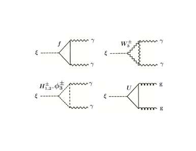
Figure 1: One loop processes involved in the decay widths $\Gamma_{gg}$ and $\Gamma_{\gamma\gamma}$. In this figure, $f=\{U,\>E^{-},\>E_{1}^{-},\>E_{2}^{-}\}$.

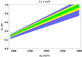
(a)

      

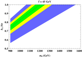
(b)

Figure 2: Contour plots of the production cross-section $\sigma(pp\to\xi\to\gamma\gamma)$ in femtobarns. The dashed line corresponds to the central value at 6 fb, and the shaded bands corresponds to regions at 68.3% (green), 95.5% (yellow) and 99.7% (light blue) C.L. exclusion limits from ATLAS and CMS combined data.

3 Diphoton decay

For the analysis of the diphoton decay, we take into account all the possible decay modes of the 750 GeV candidate. Firstly, the masses of charged Higgs bosons $H_{1,2}^{\pm}$ and $\phi_{3}^{\pm}$ are at the TeV scale, so the decay of $\xi$ at tree level into these charged Higgs bosons in the model is kinematically forbidden. Secondly, when the SSB $SU(3)_{L}\rightarrow SU(2)_{L}$ takes place, $U_{L}$ does not acquire a $SU(2)_{L}$ quantum number resulting in a $SU(2)_{L}$ singlet. As a consequence of that, the decay $\xi\rightarrow WW$ is forbidden too. Thirdly, the $\xi\rightarrow ZZ$ decay is negligible at tree-level as it is suppressed by the $Z-$mixing angle $\tan\theta_{Z}\propto{v^{2}}/{V^{2}}$. Similarly, the $\xi\rightarrow t\overline{t}$ decay is negligible at tree-level as the $\xi-t$ coupling is proportional to $\sin\theta_{tU}\propto v_{2}/V_{1}$. Finally, the decay $\xi\rightarrow hh$ is strongly constrained by ATLAS and CMS at 95%CL [34]. In this way, we obtain the following total decay width for $\xi$,

$$\Gamma=\Gamma_{\gamma\gamma}+\Gamma_{gg}+\Gamma_{Z\gamma}+\Gamma_{ZZ}.$$ (39)

The experimentally reported width of the resonance ranges between 0 and 100 GeV, and can be larger (‘broad’) or smaller (‘narrow’) than the experimental resolution of about 6-10 GeV [35]. The best-fit width reported by the ATLAS Collaboration is $\Gamma\sim 45\,\mathrm{GeV}\sim 0.06\,m_{\xi}$. So, in view of some tension with the CMS data we use three approximations for the decay width:

• A width approximation given by the experimentally reported width from the ATLAS Collaboration $\Gamma=45$ GeV.

• A width approximation for a narrower resonance with $\Gamma=1$ GeV.

• An approximation given only by one loop contributions, $\Gamma=\Gamma_{\gamma\gamma}+\Gamma_{gg}+\Gamma_{Z\gamma}+\Gamma_{ZZ}$.

Following [33, 36] the decay rates of $\xi$ are given by

$$\Gamma(\xi\to\gamma\gamma) =\frac{\alpha^{2}h_{U}^{2}m_{\xi}^{3}}{512\pi^{3}m_{U}^{2}}\big{|}\sum_{i}N_{ci}Q_{i}^{2}F_{i}\big{|}^{2},$$

$$\Gamma(\xi\to gg) =\frac{\alpha_{s}^{2}h_{U}^{2}m_{\xi}^{3}}{64\pi^{3}m_{U}^{2}}\big{|}\sum_{i}F_{i}\big{|}^{2},$$

$$\Gamma\left(\xi\to Z\gamma\right) =\frac{\alpha^{2}h_{U}^{2}m_{\xi}^{3}}{64\pi^{3}m_{U}^{2}}\left(1-\dfrac{m_{Z}^{2}}{m_{\xi}^{2}}\right)^{3}\left|\frac{7\kappa^{2}c_{w}}{2s_{w}}+\frac{2}{3}\sum_{i}N_{ci}Q_{i}^{2}+\frac{\lambda^{2}}{24\pi\alpha}\right|^{2},$$

$$\Gamma\left(\xi\to ZZ\right) =\frac{\alpha^{2}h_{U}^{2}m_{\xi}^{3}}{128\pi^{3}m_{U}^{2}}\mathcal{P}\left(\dfrac{m_{Z}^{2}}{m_{\xi}^{2}}\right)\left|\frac{7\kappa^{2}c_{w}{}^{2}}{2s_{w}{}^{2}}-\frac{2}{3}\sum_{i}N_{ci}Q_{i}^{2}-\frac{\lambda^{2}}{24\pi\alpha}-\frac{\eta^{2}}{96\pi\alpha}\right|^{2}$$ (40)

where $\mathcal{P}(x)=\sqrt{1-4x}\left(1-4x+6x^{2}\right)$ is a factor correcting the massive final states in the decay width. Here, $h_{U}^{2}=(h_{\chi 1}^{2}+h_{\psi 1}^{2})/2$ , i.e, we assume the same Yukawa coupling for the three families for simplicity and with the same mass $m_{U}$ and we have made $\kappa=\kappa^{\prime}$, $\lambda=\lambda^{\prime}$. The functions $F_{i}$

$$F_{i}(\tau_{i})=\begin{cases}2+3\tau_{i}+3\tau_{i}(2-\tau_{i})f(\tau_{i})&i=1\\ -2\tau_{i}\left[1+(1-\tau_{i})f(\tau_{i})\right]&i=1/2\\ \frac{1}{2}\tau_{i}\left[1-\tau_{i}f(\tau_{i_{i}})\right]&i=0\end{cases}$$ (41)

are spin dependent functions for the loop factor. For $\tau_{i}>1$ the function $f(\tau_{i})$ is

$$f(\tau_{i})=\left[\arcsin\left(\frac{1}{\sqrt{\tau_{i}}}\right)\right]^{2}.$$ (42)

with $\tau_{i}=4m_{i}^{2}/m_{\xi}^{2}$, where the masses of the particles into the loop are $m_{i}>375$ GeV.

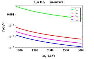
(a)

      

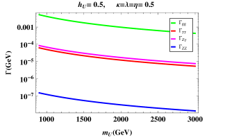
(b)

Figure 3: Different decay channels for the 750 GeV candidate at one loop level.

3.1 Production cross section

The total cross section $\sigma(pp\to\xi\to\gamma\gamma)$ in the narrow width approximation is given by

$$\sigma(pp\to\xi\to\gamma\gamma)=\frac{C_{gg}\Gamma(\xi\to gg)}{s\>m_{\xi}\Gamma}\Gamma(\xi\to\gamma\gamma).$$ (43)

where

$$C_{gg}=\frac{\pi^{2}}{8}\intop_{m_{\xi/s}}^{1}\frac{dx}{x}g(x)g(m_{\xi}^{2}/sx)$$ (44)

is the dimensionless partonic integral computed at the scale $\mu=m_{\xi}=750$ GeV and center of mass energy $\sqrt{s}=13\,\mathrm{TeV}$, obtaining $C_{gg}=2137$ [37]. For the analysis we have taken the combined-rescaled results for the cross section from CMS and ATLAS, $\sigma(pp\to\xi\to\gamma\gamma)=(2-8)\>\mathrm{fb}$ equally valid for $\sqrt{s}=8$ TeV and $C_{gg}=174$[34].

Fig. 1 shows all the possible one loop contributions from exotic charged Higgs bosons, gauge bosons and fermions. In the fermionic loop to $\gamma\gamma$ we take into account the multiplicity coming from the three families, i.e., three exotic quarks and nine exotic charged leptons. For this reason, the contribution coming from the charged Higgs bosons is almost negligible. We also take $m_{W_{3}^{\pm}}\sim 3$ TeV according to experimental constraints obtained by ATLAS and CMS Collaboration [39]. However, for $m_{W_{3}^{\pm}}\sim 3$ TeV the associated form factor $F_{1}$ reaches its asymptotic value so the cross section dependence on $m_{W_{3}^{\pm}}$ is suppressed. So, the production cross section will depend only on the Yukawa coupling $h_{U}$, the mass of the quarks $m_{U}$ and on the exotic charged lepton masses $m_{E}$, $m_{E_{1}}$ and $m_{E_{2}}$. From the lower bound reported by the ATLAS Collaboration searches on exotic heavy charged leptons [40] we set $m_{E}=m_{E_{1}}=m_{E_{2}}\sim 600$ GeV.

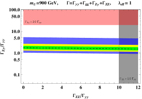
(a)

      

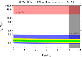
(b)

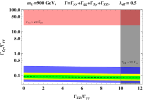
(c)

      

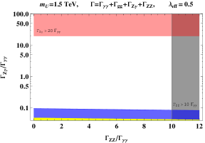
(d)

Figure 4: Contour plots of the production cross-section $\sigma(pp\to\xi\to\gamma\gamma)$ in femtobarns. The dashed line corresponds to the central value at 6 fb, and the shaded bands corresponds to regions at 68.3% (green), 95.5% (yellow) and 99.7% (light blue) C.L. exclusion limits from ATLAS and CMS combined data. The shaded red and gray regions are excluded.

Taking into account all the above conditions, we display in Fig.2 contour plots of the production cross-section $\sigma(pp\to\xi\to\gamma\gamma)$ as function of the up-type quark mass $m_{U}$ and the Yukawa coupling normalized as $h_{U}/4\pi$ for $\Gamma=1$ GeV and $\Gamma=45$ GeV. The lower bound of 900 GeV for $m_{U}$ corresponds to the reported value in recent searches on top- and bottom-like heavy quarks from ATLAS and CMS Collaborations [41] and the upper bound of 3 TeV corresponds to the asymptotic value obtained from the fermionic from factor $F_{1/2}$. We obtain allowed regions for both $\Gamma=1$ GeV and $\Gamma=45$ GeV widths for the scalar particle of 750 GeV in agreement with the ATLAS and CMS Collaborations data. In Fig.2 (a) we obtain values for $h_{U}/4\pi$ from $0.2$ to $1.0$ and an allowed mass region for the up-like quark from 900 GeV to 3.0 TeV at 99.7% CL. In Fig.2 (b) the model is excluded for $h_{U}/4\pi<0.6$ and $m_{U}>1.5$ TeV at 99.7% CL.

Finally, for the case $\Gamma=\Gamma_{\gamma\gamma}+\Gamma_{gg}+\Gamma_{Z\gamma}+\Gamma_{ZZ}$, we show in Fig. 3 the different contributions in Eq. (40) for the decay width of $\xi$. From Fig. 3 (a), the case $\kappa=\lambda=\eta=0$ and $h_{U}=0.5$ corresponds to pure fermionic contributions into the loops. We can see that the contributions (ignoring the dominant $\Gamma_{gg}$) $\Gamma_{\gamma\gamma},$ $\Gamma_{Z\gamma}$, $\Gamma_{ZZ}$ have branching ratios of order $64\%,$ $25\%$, $11\%$ respectively. On the other hand, the case $\kappa=\lambda=\eta=0.5$ and $h_{U}=0.5$ in Fig. 3 (b), corresponds to both fermionic and bosonic contributions into the loop with $\mathrm{BR}_{\gamma\gamma},$ $\mathrm{BR}_{Z\gamma}$, $\mathrm{BR}_{ZZ}$ of order $43\%,$ $56\%$, $1\%$ respectively.

In this way, and taking into account current bounds on $\Gamma_{Z\gamma}/\Gamma_{\gamma\gamma}$ and $\Gamma_{ZZ}/\Gamma_{\gamma\gamma}$ [42], we display in Fig.4 contour plots of the production cross-section $\sigma(pp\to\xi\to\gamma\gamma)$ in the $\Gamma_{Z\gamma}/\Gamma_{\gamma\gamma}$-$\Gamma_{ZZ}/\Gamma_{\gamma\gamma}$ plane. For simplicity, we have set $\lambda_{eff}\equiv\kappa=\lambda=\eta=h_{U}$ in such a way that the contour plots only depend on $m_{U}$ and $\lambda_{eff}$. In general, for low values of $m_{U}$ the ratio $\Gamma_{Z\gamma}/\Gamma_{\gamma\gamma}$ is of order $\Gamma_{Z\gamma}/\Gamma_{\gamma\gamma}\sim 1$, and for greater values of $m_{U}$ we have $\Gamma_{Z\gamma}/\Gamma_{\gamma\gamma}<1$. We also observe that the greater the ratio $\Gamma_{Z\gamma}/\Gamma_{\gamma\gamma}$, the stronger the coupling $\lambda_{eff}$. However, if $\lambda_{eff}>3$ the model is completely excluded by the bound $\Gamma_{Z\gamma}<20\Gamma_{\gamma\gamma}$ for all $m_{U}$.

4 Summary

We have presented an anomaly-free model based on the electroweak-strong unification group $SU(6)\otimes U(1)_{X}$, containing the $SU(3)_{C}\otimes SU(3)_{L}\otimes U(1)_{X}$ as a subgroup. We break the gauge symmetry down to $SU(3)_{C}\otimes U(1)_{Q}$ and at the same time give masses to the fermion fields in the model in a consistent way by five Higgs fields $\Phi$, $H_{1}$, $H_{2}$ , $H_{3}$ and $H_{S}$. These Higgs fields and their VEVs set two different mass scales: $\upsilon=256$ GeV $<<V$. From the mixing terms between the real fields $\xi_{1}$ in $H_{1}$ and $\xi_{S}$ in $H_{S}$, we obtain two real scalar fields: our candidate for the 750 GeV signal $\xi$, and one $\xi^{\prime}$ at the TeV scale. For the analysis of the diphoton decay, we take into account all the possible decay modes of the 750 GeV candidate considering three approximations for the decay width: $\Gamma=1$ GeV, $\Gamma=45$ GeV and $\Gamma=\Gamma_{\gamma\gamma}+\Gamma_{gg}+\Gamma_{Z\gamma}+\Gamma_{ZZ}$. Then, taking various simplified assumptions on the parameter space, we show that the states $U$, $E$, $E_{1}$, $E_{2}$, $W_{3}^{\pm}$, $H_{1,2}^{\pm}$ and $\phi_{3}^{\pm}$ into the loop can explain the diphoton excess for each one of the width approximations according to ATLAS and CMS bounds on all the particle masses involved and on the decay widths $\Gamma_{Z\gamma}$ and $\Gamma_{ZZ}$.

References

- [1] Talk by Jim Olsen, CMS Collaboration, “CMS 13 TeV Results", CERN Jamboree, December 15, 2015. Plots are presented in, http://cms-results.web.cern.ch/cms-results/public-results/preliminary-results/LHC-Jamboree-2015/index.html.
- [2] Talk by Marumi Kado, ATLAS Collaboration, “ATLAS 13 TeV Results", CERN Jamboree, December 15, 2015. Plots are presented in, https://twiki.cern.ch/twiki/bin/view/ AtlasPublic/December2015-13TeV .
- [3] K. Harigaya and Y. Nomura, arXiv:1512.04850; Y. Mambrini, G. Arcadi and A. Djouadi, arXiv:1512.04913; M. Backovic, A. Mariotti and D. Redigolo, arXiv:1512.04917; A. Angelescu, A. Djouadi and G. Moreau, arXiv:1512.04921; Y. Nakai, R. Sato and K. Tobioka, arXiv:1512.04924; S. Knapen, T. Melia, M. Papucci and K. Zurek, arXiv:1512.04928; D. Buttazzo, A. Greljo and D. Marzocca, arXiv:1512.04929; A. Pilaftsis, arXiv:1512.04931; R. Franceschini et al., arXiv:1512.04933; S. D. McDermott, P. Meade and H. Ramani, arXiv:1512.05326; R. Benbrik, C.-H. Chen, T. Nomura, arXiv:1512.06028; J. Ellis, et al., arXiv:1512.05327; M. Low, A. Tesi and L.-T. Wang, arXiv:1512.05328; B. Bellazzini, R. Franceschini, F. Sala and J. Serra, arXiv:1512.05330; R. S. Gupta, et al., arXiv:1512.05332; C. Peterson and R. Torre, arXiv:1512.05333; E. Molinaro, F. Sannino and N. Vignaroli, arXiv:1512.05334.
- [4] B. Dutta, et al., arXiv:1512.05439; Q.-H. Cao, et al., arXiv:1512.05542; S. Matsuzaki and K. Yamawaki, arXiv:1512.05564; A. Kobakhidze, et al., arXiv:1512.05585; R. Martinez, F. Ochoa and C. F. Sierra, arXiv:1512.05617; P. Cox, A. D. Medina, T. S. Ray and A. Spray, arXiv:1512.05618; D. Becirevic, E. Bertuzzo, O. Sumensari and R. Z. Funchal, arXiv:1512.05623; J. M. No, V. Sanz and J. Setford, arXiv:1512.05700; S. V. Demidoz and D. S. Gorunov, arXiv:1512.05723; W. Chao, R. Huo and J. Yu, arXiv:1512.05738; S. Fichet, G. V. Gersdorff and C. Royon, arXiv:1512.05751; D. Curtin, C. B. Verhaaren, arXiv:1512.05753, L. Bian, N. Chen, D. Liu and J. Shu, arXiv:1512.05759; J. Chakrabortty, et al., arXiv:1512.05767; A. Ahmed, et al., arXiv:1512.05771; C. Csaki, J. Hubisz and J. Terning, arXiv:1512.05776; A. Falkowski, O. Slone and T. Volaksky, arXiv:1512.05777; D. Aloni, et al., arXiv:1512.05778; Y. Bai, J. Berger and R. Lu, arXiv:1512.05779.
- [5] E. Gabrielli, et al., arXiv:1512.05961; J. S. Kim, J. Reuter, K. Rolbiecki and R. R. de Austri, arXiv:1512.06083; A. Alves, A. G. Dias and K. Sinha, arXiv:1512.06091; E. Megias, O. Pujolas and M. Quiros, arXiv:1512.06106; L. M. Carpenter, R. Colburn and J. Goodman, arXiv:1512.06107; J. Bernon and C. Smith, arXiv:1512.06113; W. Chao, arXiv:1512.06297; M. T. Arun and P. Saha, arXiv:1512.06335; C. Han, H. M. Lee, M. Park and V. Sanz, arXiv:1512.06376; S. Chang, arXiv:1512.06426; M. Luo, et al., arXiv:1512.06670.
- [6] I. Chakraborty and A. Kundu, arXiv:1512.06508; R. Ding, L. Huang, T. Li and B. Zhu, arXiv:1512.06560; H. Han, S. Wang and S. Zheng, arXiv:1512.06562; X. -F. Han and L. Wang, arXiv:1512.06587; J. Chang, K. Cheung and C. Lu, arXiv:1512.06671; D. Bardhan, et al., arXiv:1512.06674; T.-F. Feng, X.-Q. Li, H.-B. Zhang and S.-M. Zhao, arXiv:1512.06696; O. Antipin, M. Mojaza and F. Sannino, arXiv:1512.06708; F. Wang, L. Wu, J. M. Yang and M. Zhang, arXiv:1512.06715; J. Cao, et al., arXiv:1512.06728; F. P. Huang, C. S. Li, Z. L. Liu and Y. Wang, arXiv:1512.06732; W. Liao and H. -Q. Zheng, arXiv:1512.06741; J. J. Heckman, arXiv:1512.06773; M. Dhuria and G. Goswami, arXiv:1512.06782; X.-J. Bi, Q. -F. Xiang, P.-F. Yin and Z.-H. Yu, arXiv:1512.06787; J. S. Kim, K. Rollbiecki and R. R. de Austri, arXiv:1512.06797; L. Berthier, J. M. Cline, W. Shepherd and M. Trott, arXiv:1512.06799; W. S. Cho et al., arXiv:1512.06824; J. M. Cline and Z. Liu, arXiv:1512.06827; M. Bauer and M. Neubert, arXiv:1512.06828; M. Chala, M. Duerr, F. Kahlhoefer and K. S. Hoberg, arXiv:1512.06833; D. Barducci et al. arXiv:1512.06842.
- [7] S. M. Boucenna, S. Morisi and A. Vicente, arXiv:1512.06878; C. W. Murphy, arXiv:1512.06976; A. E. C. Hernandez and I. Nisandzic, arXiv:1512.07165; U. K. Dey, S. Mohanty and G. Tomar, arXiv:1512.07212; G. M. Pelaggi, A. Strumia, E. Vigiani, arXiv:1512.07225; J. de Blas, J. Santiago and R. V. -Morales, arXiv:1512.07229; A. Belyaev, et al., arXiv:1512.07242; P. S. B. Dev and D. Teresi, arXiv:1512.07243; W.-C. Huang, Y. Tsai and T.-C. Yuan, arXiv:1512.07268; S. Moretti and K. Yagyu, arXiv:1512.07462; K. M. Patel and P. Sharma, arXiv:1512.7468; M. Badziak, arXiv:1512.07497; S. Chakraborty, A. Chakraborty and S. Raychaudhuri, arXiv:1512.07527; W. Altmannshoefer, et al., arXiv:1512.07616; M. Cvetic, J. Halverson and P. Langacker, arXiv:1512.07622; J. Gu and Z. Liu, arXiv:1512.07624.
- [8] Q.-H. Cao, S.-L. Chen and P.-H. Gu, arXiv:1512.07541; P. Dev, R. N. Mohapatra and Y. Zhang, arXiv:1512.08507; B. C. Allanach, P. Dev, S. A. Renner and K. Sakurai, arXiv:1512.07645; H. Davoudiasl and C. Zhang, arXiv:1512.07672; N. Craig, P. Draper, C. Kilic and S. Thomas, arXiv:1512.07733; K. Das and S. K. Rai, arXiv:1512.07789; K. Cheung, et al., arXiv:1512.07853; J. Liu, X.-P. Wang and W. Xue, arXiv:1512.07885; J. Zhang and S. Zhou, arXiv:1512.07889; J. A. Casas, J. R. Espinosa and J. M. Moreno, arXiv:1512.07895; L. J. Hall, K. Harigaya and Y. Nomura, arXiv:1512.07904.
- [9] H. Han, S. Wang, S. Zheng and S. Zheng, arXiv:1512.07992; J.-C. Park and S. C. Park, arXiv:1512.08117; A. Salvio and A. Mazumdar, arXiv:1512.08184; D. Chway, R. Dermivsek, T. H. Jung and H. D. Kim, arXiv:1512.08221; G. Lo, et al., arXiv:1512.08255; M. Son and A. Urbano, arXiv:1512.08307; Y.-L. Tang and S.-H. Zhu, arXiv:1512.08323; H. An, C. Cheung and Y. Zhang, arXiv:1512.08378; J. Cao, F. Wang and Y. Zhang, arXiv:1512.08392; F. Wang, et al., arXiv:1512.08434; C. Cai, Z.-H. Yu and H. Zhang, arXiv:1512.08440; Q.-H. Cao, et al., arXiv:1512.08441; J. E. Kim, arXiv:1512.08467; J. Gao, H. Zhang and H. X. Zhu, arXiv:1512.08478; W. Chao, arXiv:1512.08484; X.-J. Bi, et al., arXiv:1512.08497; F. Goertz, J. F. Kamenik, A. Katz and M. Nardecchia, arXiv:1512.08500; L. A. Anchordoqui, I. Antoniadis, H. Goldberg and X. Huang, arXiv:1512.08502; N. Bizot, S. Davidson, M. Frigerio and J.-L. Kneur, arXiv:1512.08508; K. Kaneta, S. Kang, H.-S. Lee, arXiv:1512.09129; I. Low, J. Lykken, arXiv:1512.09089.
- [10] L. E. Ibanez, V. M. Lozano, arXiv:1512.08777; E. Ma, arXiv:1512.09159; L. Marzola, et al., arXiv:1512.09136; Y. Jiang, Y.-Y. Li, T. Liu, arXiv:1512.09127; A. E. C. Hernandez, arXiv:1512.09092; S. Kanemura, N. Machida, S. Odori, T. Shindou, arXiv:1512.09053; S. Kanemura, et al., arXiv:1512.09048; X.-J. Huang, W.-H. Zhang, Y.- F. Zhou, arXiv:1512.08992; Y. Hamada, T. Noumi, S. Sun, G. Shiu, arXiv:1512.08984; S. K. Kang, J. Song, arXiv:1512.08963; C.-W. Chiang, M. Ibe, T. T. Yanagida, arXiv:1512.08895; A. Dasgupta, M. Mitra, D. Borah, arXiv:1512.09202.
- [11] A. E. Faraggi, J. Rizos, arXiv:1601.03604; A. Djouadi, J. Ellis, R. Godbole, J. Quevillon, arXiv:1601.03696; J. H. Davis, M. Fairbairn, J. Heal, P. Tunney, arXiv:1601.03153; R. Ding, Z.-L. Han, Y. Liao, X.-D. Ma, arXiv:1601.02714; M. Fabbrichesi, A. Urbano, arXiv:1601.02447; J. Cao, et al., arXiv:1601.02570; P. Ko, T. Nomura, arXiv:1601.02490; S. Fichet, G. v. Gersdorff, C. Royon, arXiv:1601.01712; I. Sahin, arXiv:1601.01676; D. Borah, S. Patra, S. Sahoo, arXiv:1601.01828; S. Bhattacharya, S. Patra, N. Sahoo, N. Sahu, arXiv:1601.01569; F. DEramo, J. de Vries, P. Panci, arXiv:1601.01571; H. Ito, T. Moroi, Y. Takaesu, arXiv:1601.01144; A. E. C. Hernandez, I. d. M. Varzielas, E. Schumacher, arXiv:1601.00661; T. Modak, S. Sadhukhan, R. Srivastava, arXiv:1601.00836; C. Csaki, J. Hubisz, S. Lombardo, J. Terning, arXiv:1601.00638; U. Danielsson, R. Enberg, G. Ingelman, T. Mandal, arXiv:1601.00624; D. Palle, arXiv:1601.00618; K. Ghorbani, H. Ghorbani, arXiv:1601.00602; X-F. Han, et al., arXiv:1601.00534; E. Palti, arXiv:1601.00285; P. Ko, Y. Omura, C. Yu, arXiv:1601.00586; T. Nomura, H. Okada, arXiv:1601.00386; H. Zhang, arXiv:1601.01355; S. Jung, J. Song, Y. W. Yoon, arXiv:1601.00006; I. Dorsner, S. Fajfer, N. Kosnik, arXiv:1601.03267; C. Hati, arXiv:1601.02457; D. Stolarski, R. V.- Morales, arXiv:1601.02004; A. Berlin, arXiv:1601.01381; F. F. Deppisch, C. Hati, S. Patra, P. Pritimita, U. Sarkar, arXiv:1601.00952; B. Dutta, et al., arXiv:1601.00866; A. Karozas, S.F. King, G. K. Leontaris, A. K. Meadowcroft, arXiv:1601.00640; W. Chao, arXiv:1601.00633; arXiv:1601.04678; C. T. Potter, arXiv:1601.00240; A. Ghoshal, arXiv:1601.04291; T. Nomura, H. Okada, arXiv:1601.04516; Ufuk Aydemir, Tanumoy Mandal, arXiv:1601.06761 [hep-ph].
- [12] S. Cecotti et al, Phys. Lett. B156, 318 (1985); G. Lazarides and Q. Shafi, Nucl. Phys. B329, 183 (1990); B338, 442 (1990); C. Panagiotakopoulos, Int. J. Mod. Phys. A5, 2359 (1990).
- [13] R. Martinez, William A. Ponce, Luis A. Sanchez, Phys.Rev.D65:055013, (2002).
- [14] C. Panagiotakopoulos, Physics Letters B269, 71-76 (1991).
- [15] K. Inoue, A. Kakuto and T. Takano, Progr. Theor. Phys. 75 (1986) 664; A. Anselm and A. Johansen, Phys. Lett. B200 (1988) 331; Z. Berezhiani and G. Dvali, Sov. Phys. Lebedev Institute Reports 5 (1989) 55.
- [16] R. Barbieri, G. Dvali and A. Strumia, Nucl. Phys. B391 (1993) 487; R. Barbieri, G. Dvali and M. Moretti, Phys. Lett. B312 (1993) 137; R. Barbieri, G. Dvali, A. Strumia, Z. Berezhiani, L.Hall, Nucl.Phys. B432 (1994) 49; Z. Berezhiani, Phys. Lett. B355 (1995) 481; Z. Berezhiani, C. Csaki and L. Randall, Nucl. Phys. B444 (1995) 61; G. Dvali and S. Pokorski, Phys. Rev. Lett. 78 (1997) 807.
- [17] G. Dvali and Q. Shafi, Phys. Lett. B326 (1994) 258; B339 (1994) 241.
- [18] S. Barr, Phys. Lett. B112 (1982) 219; Phys. Rev. D40 (1989) 2457; J.-P. Derendinger, J. Kim and D.V. Nanopoulos, Phys. Lett. B139 (1984)170.
- [19] I. Antoniadis, J. Ellis, S. Hagelin and D.V. Nanopoulos, Phys. Lett. B194 (1987) 231; Phys. Lett. B231 (1987) 65.
- [20] J. Ellis, D.V. Nanopoulos, K. Olive, Phys.Lett.B300, 121-127 (1993).
- [21] Q. Shafi, Zurab Tavartkiladze, Nucl.Phys.B552, 67-87 (1999).
- [22] F. Pisano and V. Pleitez, Phys. Rev. D46, 410 (1992); R. Foot, O.F. Hernandez, F. Pisano, V. Pleitez, Phys. Rev. D47, 4158 (1993); V. Pleitez and M.D. Tonasse, Phys. Rev. D48, 2353 (1993); Nguyen Tuan Anh, Nguyen Anh Ky, Hoang Ngoc Long, Int. J. Mod. Phys. A16, 541 (2001).
- [23] P.H. Frampton, Phys. Rev. Lett. 69, 2889 (1992); P.H. Frampton, P. Krastev and J.T. Liu, Mod. Phys. Lett. 9A, 761 (1994); P.H. Frampton et. al. Mod. Phys. Lett. 9A, 1975 (1994)
- [24] R. Foot, H.N. Long and T.A. Tran, Phys. Rev. D50, R34 (1994); H.N. Long, ibid. 53, 437 (1996); ibid, 54, 4691 (1996); Mod. Phys. Lett. A13, 1865 (1998); Nguyen Anh Ky, Hoang Ngoc Long, Int. J. Mod. Phys. A16, 541 (2001)
- [25] Rodolfo A. Diaz, R. Martinez, F. Ochoa, Phys. Rev. D69, 095009 (2004); Rodolfo A. Diaz, R. Martinez, F. Ochoa, Phys. Rev. D72, 035018 (2005); Fredy Ochoa, R. Martinez, Phys. Rev D72, 035010 (2005).
- [26] E. Ma and G. Rajasekaran, Phys. Rev. D 64, 113012 (2001); K. S. Babu, E. Ma and J. W. F. Valle, Phys. Lett. B 552, 207 (2003).
- [27] G. Altarelli, F. Feruglio, L. Merlo, Tri-Bimaximal Neutrino Mixing and Discrete Flavor Symmetries, arXiv: 1205.5133v3[hep-ph].
- [28] A. E. Carcamo Hernandez, R. Martinez, arXiv:1501.05937v2 [hep-ph].
- [29] Wyler, D., and Wolfenstein, L., Nucl. Phys. B 218, 205 (1983).
- [30] Mohapatra, R. N., and Valle, J. W. F., Phys. Rev. D 34, 1642 (1986).
- [31] ’t Hooft, G., 1980, in Proceedings of 1979 Carg‘ese Institute on Recent Developments in Gauge Theories, edited by ’t Hooft, G., et al. (Plenum Press, New York), p. 135.
- [32] E. Catano M., R Martinez, and F. Ochoa, Phys. Rev. D 86, 073015 (2012).
- [33] Qing-Hong Cao, Yandong Liu, Ke-Pan Xie, Bin Yan, Dong-Ming Zhang, Phys. Rev. D93, 075030 (2016).
- [34] John Ellis, Sebastian A. R. Ellis, J. Quevillon, Veronica Sanz, Tevong You, arXiv:1512.05327.
- [35] Alessandro Strumia, arXiv:1605.09401 [hep-ph].
- [36] J.F. Gunion, H.E. Haber, G. Kane and S. Dawson. The Higgs Hunter’s Guide. Addison-Wesley Publishing Company. 1990; R. Martinez, M. A. Perez, and J. J. Toscano, Phys. Rev. D 40, 1722 (1989); R. Martinez, M.A. Perez, J.J. Toscano, Phys.Lett. B234 (1990) 503; R. Martinez, M.A. Perez, Nucl.Phys. B347 (1990) 105-119.
- [37] A.D. Martin, W.J. Stirling, R.S. Thorne, G. Watt, “Parton distributions for the LHC”, Eur. Phys. J. C63 (2009) 189 [arXiv:0901.0002].
- [38] Stefano Di Chiara, Luca Marzola, Martti Raidal, arXiv:1512.04939.
- [39] ATLAS Collaboration, JHEP 12, 55 (2015) ; CMS Collaboration, “Search for leptonic decays of W’ bosons in pp collisions at = 8 TeV”, report CMS-PAS-EXO-12-060, March 2013.
- [40] ATLAS Collaboration, Phys. Rev. D 92, 032001 (2015).
- [41] CMS Collaboration, Phys. Rev. D 93, 012003 (2016); ATLAS Collaboration, arXiv:1602.05606 [hep-ex]; CMS Collaboration arXiv:1507.07129 [hep-ex].
- [42] Roberto Franceschini, Gian F. Giudice, Jernej F. Kamenik, Matthew McCullough, Francesco Riva, Alessandro Strumia, Riccardo Torre, arXiv:1604.06446 [hep-ph].