Perceptual Vector Quantization for Video Coding

Abstract

This paper applies energy conservation principles to the Daala video codec using gain-shape vector quantization to encode a vector of AC coefficients as a length (gain) and direction (shape). The technique originates from the CELT mode of the Opus audio codec, where it is used to conserve the spectral envelope of an audio signal. Conserving energy in video has the potential to preserve textures rather than low-passing them. Explicitly quantizing a gain allows a simple contrast masking model with no signaling cost. Vector quantizing the shape keeps the number of degrees of freedom the same as scalar quantization, avoiding redundancy in the representation. We demonstrate how to predict the vector by transforming the space it is encoded in, rather than subtracting off the predictor, which would make energy conservation impossible. We also derive an encoding of the vector-quantized codewords that takes advantage of their non-uniform distribution. We show that the resulting technique outperforms scalar quantization by an average of 0.90 dB on still images, equivalent to a 24.8% reduction in bitrate at equal quality, while for videos, the improvement averages 0.83 dB, equivalent to a 13.7% reduction in bitrate.

1 Introduction

Video codecs are traditionally based on scalar quantization of discrete cosine transform (DCT) coefficients with uniform quantization step sizes. High-quality encoders signal quantization step size changes at the macroblock level to account for contrast masking [1]. The adjustment cannot be applied at a level smaller than a full macroblock and applies to all frequencies uniformly. Audio codecs have long considered frequency-dependent masking effects and more recently, the Opus codec [2] has integrated masking properties as part of its bitstream in a way that does not require explicit signaling.

We apply the same principles to the Daala video codec [3], using gain-shape vector quantization to conserve energy. We represent each vector of AC coefficients by a length (gain) and a direction (shape). The shape is an $N$-dimensional vector that represents the coefficients after dividing out the gain. The technique originates from the CELT mode [4] of the Opus audio codec, where splitting the spectrum into bands and coding an explicit gain for each band preserves the spectral envelope of the audio. Similarly, conserving energy in videohas the potential to preserve textures rather than low-passing them. Explicitly quantizing a gain allows a simple contrast masking model with no signaling cost. Vector quantizing the shape keeps the number of degrees of freedom the same as scalar quantization, avoiding redundancy in the representation.

Unlike audio, video generally has good predictors available for the coefficients it is going to code, e.g., the motion-compensated reference frame. The main challenge of gain-shape quantization for video is figuring out how to apply that prediction without losing the energy-conserving properties of explicitly coding the gain of the input vector. We cannot simply subtract the predictor from the input vector: the length of the resulting vector would be unrelated to the gain of the input. That is, the probability distribution of the points on the hypersphere is highly skewed by our predictor, rather than being fixed, like in CELT. Section 3 shows how to transform the hypersphere in a way that allows us to easily model this skew. Finally, we derive a new way of encoding the shape vector that accounts for the fact that low-frequency AC coefficients have a larger variance than high-frequency AC coefficients. We then compare the quality obtained using the proposed technique to scalar quantization on both still images and videos.

2 Gain-Shape Quantization

Most video and still image codecs use scalar quantization. That is, once the image is transformed into frequency-domain coefficients, they quantize each (scalar) coefficient separately to an integer index. Each index represents a certain scalar value that the decoder uses to reconstruct the image. For example, using a quantization step size of 10, a decoder receiving indices -2, +4, produces reconstructed coefficients of -20, +40, respectively. Scalar quantization has the advantage that each dimension can be quantized independently from the others.

With vector quantization, an index no longer represents a scalar value, but an entire vector. The possible reconstructed vectors are no longer constrained to the regular rectangular grid above, but can be arranged in any way we like, either regularly, or irregularly. Each possible vector is called a codeword and the set of all possible codewords is called a codebook. The codebook may be finite if we have an exhaustive list of all possibilities, or it can also be infinite in cases where it is defined algebraically (e.g., scalar quantization is equivalent to vector quantization with a particular infinite codebook).

Gain-shape vector quantization represents a vector by separating it into a length and a direction. The gain (the length) is a scalar that represents how much energy is in the vector. The shape (the direction) is a unit-norm vector that represents how that energy is distributed in the vector. In two dimensions, one can construct a gain-shape quantizer using polar coordinates, with gain being the radius and the shape being the angle. In three dimensions, one option (of many) is to use latitude and longitude for the shape. In Daala, we don’t restrict ourselves to just two or three dimensions. For a 4x4 transform, we have 16 DCT coefficients. We always code the DC separately, so we are left with a vector of 15 AC coefficients to quantize. If we quantized the shape vector with scalar quantization, we would have to code 16 values to represent these 15 coefficients: the 15 normalized coefficients plus the gain. That would be redundant and inefficient. But by using vector quantization, we can code the direction of an $N$-dimensional vector with $(N-1)$ degrees of freedom, just like polar coordinates in 2-D and latitude and longitude in 3-D. Classically, vector quantization provides other advantages, such as the space filling advantage, the shape advantage, and the memory advantage [5], but we benefit very little, if at all, from these. Our primary interest is in elminating redundancy in the encoding.

In Daala, as in CELT, we use a normalized version of the pyramid vector quantizer described by Fischer [6] for the shape codebook. Fischer’s codebook is defined as the set of all $N$-dimensional vectors of integers where the absolute value of the integers sum to $K$:

$$\mathbf{y}\in\mathbb{Z}^{N}:\sum_{i=0}^{N-1}\left|y_{i}\right|=K\ .$$ (1)

$K$ is called the number of pulses because one can think of building such a vector by distributing $K$ different pulses of unit amplitude, one at a time, among the $N$ dimensions. The pulses can point in either the positive or negative direction, but all of the ones in the same dimension must point in the same direction. For $N=2$ and $K=2$, our codebook has 8 entries:

$$(2,0),\ (-2,0),\ (1,1),\ (1,-1),\ (-1,1),\ (-1,-1),\ (0,2),\ (0,-2)$$

The normalized version of the codebook simply normalizes each vector to have a length of 1. If $\mathbf{y}$ is a codeword in Fischer’s non-normalized codebook, then the corresponding normalized vector is simply

$$\mathbf{u}=\mathbf{y}/\left\|\mathbf{y}\right\|_{L2}\ .$$ (2)

The advantages of this codebook are that it is flexible (any value of $K$ will work), it does not require large lookup tables for each $K$, and it is easy to search. Its regularity means that we can construct vectors on the fly and don’t have to examine every vector in the codebook to find the best representation for our input.

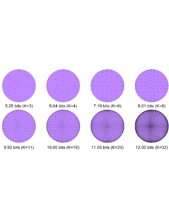
Figure 1: Normalized-pyramid vector quantizer in three dimensions. The codewords are spread relatively uniformly on the sphere (perfect uniformity is provably impossible in 3 dimensions, and not actually desirable for Laplacian sources).

The number of dimensions, $N$, is fixed, so the parameter $K$ determines the quantization resolution of the codebook (i.e., the spacing between codewords). As the gain of our vector increases, we need more points on our $N$-dimensional sphere to keep the same quantization resolution, so $K$ must increase as a function of the gain.

For the gain, we can use simple scalar quantization:

$$\hat{g}=\gamma Q\ ,$$ (3)

where $Q$ is the quantization step size, $\gamma$ is the quantization index, and $\hat{g}$ is the reconstructed (quantized) gain.

3 Prediction

Video codecs rarely code blocks from scratch. Instead, they use inter- or intra-prediction. In most cases, that prediction turns out to be very good, so we want to make full use of it. The naive approach is to just subtract the prediction from the coefficients being coded, and then apply gain-shape quantization to the residual. While this can work, we lose some of the benefits of gain-shape quantization because the gain no longer represents the contrast of the block being coded, only how much the image changed compared to the prediction.

An early attempt at warping the shape codebook [7] to increase resolution close to the prediction gave little benefit despite the increase in complexity. In this work, we instead transform the space so that the predictor lies along one of the axes, allowing us to treat that axis as “special”. This gives us much more direct control over the quantization and probability modeling of codewords close to the predictor than the codebook warping approach. We compute the transform using a Householder reflection, which is also computationally cheaper than codebook warping. The Householder reflection constructs a reflection plane that turns the prediction into a vector with only one non-zero component. Let $\mathbf{r}$ be the vector containing the prediction coefficients. The Householder reflection is defined by a vector that is normal to the reflection plane:

$$\mathbf{v}=\frac{\mathbf{r}}{\left\|\mathbf{r}\right\|}+s\mathbf{e}_{m}\,,$$ (4)

where $\mathbf{e}_{m}$ is a unit vector along axis $m$, $s=\mathrm{sign\left(r_{m}\right)}$ and axis $m$ is selected based on the largest component of the prediction, to minimize numerical error. The decoder can compute both values without sending any additional side information. The input vector $\mathbf{x}$ is reflected using $\mathbf{v}$ by computing

$$\mathbf{z}=\mathbf{x}-2\frac{\mathbf{v}^{T}\mathbf{x}}{\mathbf{v}^{T}\mathbf{v}}\mathbf{v}\ .$$ (5)

Fig. 2 illustrates the process. From this point, we focus on quantizing $\mathbf{z}$, knowing that its direction is likely to be close to $\mathbf{e}_{m}$.

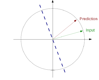
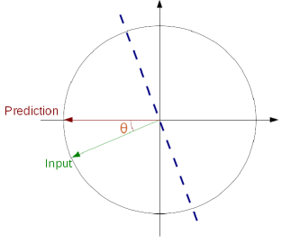
Figure 2: Householder reflection in 2 dimensions. Left: original prediction and input $\mathbf{x}$. Right: reflected input $\mathbf{z}$.

Once the prediction is aligned along an axis, we can code how well it matches the input vector using an angle $\theta$, with

$$\cos\theta=\frac{\mathbf{x}^{T}\mathbf{r}}{\left\|\mathbf{x}\right\|\left\|\mathbf{r}\right\|}=\frac{\mathbf{z}^{T}\mathbf{r}}{\left\|\mathbf{z}\right\|\left\|\mathbf{r}\right\|}=-\frac{sz_{m}}{\left\|\mathbf{z}\right\|}$$ (6)

The position of the input vector along the prediction axis on the unit hypersphere is simply $\cos\theta$, and the distance between the input and the prediction axis is $\sin\theta$. We could choose to code $\cos\theta$, or $1-\cos\theta$, or $\sin\theta$, but directly coding $\theta$ using scalar quantization turns out to be the optimal choice for minimizing mean-squared error (MSE).We then apply gain-shape quantization to the remaining dimensions, knowing that the gain of the remaining coefficients is just the original gain multiplied by $\sin\theta$. The quantized coefficients are reconstructed from the gain $\hat{g}$, the angle $\hat{\theta}$, and a unit-norm codeword $\mathbf{u}$ as

$$\mathbf{\hat{z}}=\hat{g}\left(\cos\hat{\theta}\mathbf{e}_{m}+\sin\hat{\theta}\mathbf{u}\right)\ ,$$ (7)

where $\hat{g}$, $\hat{\theta}$, and $\mathbf{u}$ are jointly rate-distortion-optimized in the encoder. Because of the angle $\hat{\theta}$, dimension $m$ can be omitted from $\mathbf{u}$, which now has $N-1$ dimensions and $N-2$ degrees of freedom (since its norm is unity). Thus the total number of degrees of freedom we have to encode for an $N$-dimensional vector remains $N$. Although one might expect the Householder reflection to distort the statistics of the coefficients in the $N-1$ dimensions remaining in $\mathbf{u}$ in unpredictable ways, since high-variance LF coefficients could be mixed with low-variance HF coefficients, in practice we find they remain relatively unchanged.

4 Activity Masking

Video and still image codecs have long taken advantage of the fact that contrast sensitivity of the human visual system depends on the spatial frequency of a pattern. The contrast sensitivity function is to vision what the absolute threshold of hearing is to audition.

Another factor that influences our perception of contrast is the presence of more contrast at the same location. We call this activity masking. It is the visual equivalent of auditory masking, where the presence of a sound can mask another sound. While auditory masking has been at the center of all audio coding technology since the 80s [8], the use of activity masking in video coding is comparatively new and less advanced. This is likely due to the fact that activity masking effects are much less understood than auditory masking, which has been the subject of experiments since at least the 30s [9].

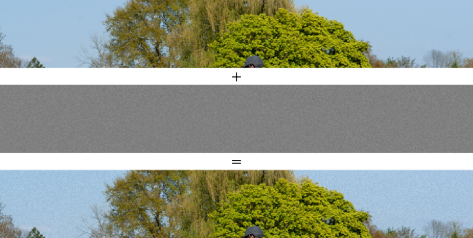
Figure 3: Contrast-dependent masking of noise. Top: original image. Middle: spatially uniform noise. Bottom: noisy image. The noise added to the bottom image is clearly visible in the sky area because of the lack of texture in that part of the original image. On the other hand, it is barely visible in the trees because it is masked by the texture present in the original image.

Fig. 3 demonstrates activity masking and how contrast in the original image affects our perception of noise. Taking into account activity masking has two related, but separate goals:

• Increasing the amount of quantization noise in high-contrast regions of the image, while decreasing it in low-contrast regions; and

• Ensuring that low-contrast regions of the image do not get completely washed out (i.e. keeping some AC).

Together, these two tend to make bit allocation more uniform throughout the frame, though not completely uniform — unlike CELT, which has uniform allocation due to the logarithmic sensitivity of the ear.

We want to make the quantization noise vary as a function of the original contrast, typically using a power law. In Daala, we make the quantization noise follow the amount of contrast raised to the power $\alpha=1/3$. We can control the resolution of the shape quantization simply by controlling the value of $K$ as a function of the gain. For gain quantization we can derive a scalar quantizer based on quantization index $\gamma$ that follows the desired resolution:

$$\frac{\partial\hat{g}}{\partial\gamma} =Q\hat{g}^{\alpha}$$

$$\hat{g}^{-\alpha}\partial\hat{g} =Q\partial\gamma$$

$$\frac{\hat{g}^{1-\alpha}}{1-\alpha} =Q\gamma$$

$$\hat{g} =\left(\left(1-\alpha\right)Q\gamma\right)^{1/\left(1-\alpha\right)}$$

$$\hat{g} =Q_{g}\gamma^{1/\left(1-\alpha\right)}$$ (8)

$$\hat{g} =Q_{g}\gamma^{\beta}$$ (9)

where $Q_{g}=\left(\left(1-\alpha\right)Q\right)^{\beta}$ is the new gain resolution and “master” quality parameter and $\beta=1/\left(1-\alpha\right)$ controls the activity masking. The effect of activity masking on our gain quantizer is equivalent to a uniform scalar quantizer applied to the companded gain. The encoder compands the gain by raising it to the power $\left(1-\alpha\right)$, and the decoder expands it back by raising it to the power $1/\left(1-\alpha\right)$. This results in a better resolution close to $g=0$ and worse resolution as the gain increases, as shown in Fig. 4. Fig. 5 shows the effect of activity masking on the spherical codebook.

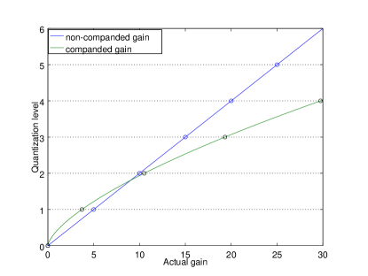
Figure 4: Gain companding example for $Q=5$. For small gains, the quantization levels result in a small change to the gain, but for large gains, the the interval is larger.

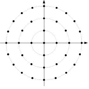
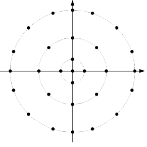
Figure 5: Effect of activity masking on the codebook. Left: no activity masking ($\alpha=0$). Right: with activity masking ($\alpha=1/3$).

When using prediction, it is important to apply the gain companding to the original $N$-dimensional coefficient vector rather than to the $N-1$ remaining coefficients after prediction. In practice, we only want to consider activity masking in blocks that have texture rather than edges. The easiest way to do this is to assume all 4x4 blocks have edges and all 8x8 to 32x32 blocks as having texture. Also, we currently only use activity masking for luma because chroma masking is much less well-understood. For blocks where we disable activity masking, we still use the same quantization described above, but set $\alpha=0$.

5 Coding Resolution

It is desirable for a single quality parameter to control $K$ and the resolution of the gain and $\theta$. That quality parameter should also take into account activity masking. The MSE-optimal angle quantization resolution is the one that matches the gain resolution. Assuming the vector distance is approximately equal to the arc distance, we have

$$Q_{\theta}=\frac{\partial\hat{g}/\partial\gamma}{\hat{g}}=\frac{Q_{g}\beta\gamma^{\beta-1}}{Q_{g}\gamma^{\beta}}=\frac{\beta}{\gamma}\ .$$ (10)

The quantized angle is thus given by

$$\hat{\theta}=Q_{\theta}\tau\ ,$$ (11)

where $\tau$ is the angle quantization index. In practice, we round $Q_{\theta}$ to an integer fraction of $\pi/2$.

5.1 Setting $K$

Using an i.i.d. Laplace source normalized to unit norm, we simulated quantization with different values of $N$ and $K$. The resulting distortion is shown in Fig. 6. The asymptotic distortion for large values of $K$ is approximately

$$D_{pvq}=\frac{\left(N-1\right)^{2}+C_{K}\left(N-1\right)}{24K^{2}}\ ,$$ (12)

with $C_{K}=4.$

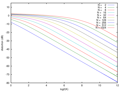
Figure 6: PVQ distortion as a function of $N$ and $K$ for a Laplace-distributed source

The distortion due to scalar quantization of the gain is (asymptotically)

$$D_{g} =\frac{1}{12}\left(\partial\hat{g}/\partial\gamma\right)^{2}$$

$$=\frac{\beta^{2}Q_{g}^{2}\gamma^{2\beta-2}}{12}\ .$$ (13)

To achieve uniform distortion along all dimensions, the distortion due to the $N-2$ PVQ degrees of freedom must be $N-2$ times greater than that due to quantizing the gain, so

$$\left(N-2\right)D_{g} =\left(\hat{g}\sin\hat{\theta}\right)^{2}D_{pvq}$$

$$\frac{\left(N-2\right)\beta^{2}Q_{g}^{2}\gamma^{2\beta-2}}{12} =\left(Q_{g}\gamma^{\beta}\sin\hat{\theta}\right)^{2}\frac{\left(N-2\right)^{2}+C_{K}\left(N-2\right)}{24K^{2}}$$

$$\left(N-2\right)\beta^{2} =\frac{\gamma^{2}\sin^{2}\hat{\theta}\left[\left(N-2\right)^{2}+C_{K}\left(N-2\right)\right]}{2K^{2}}$$

$$K =\frac{\gamma\sin\hat{\theta}}{\beta}\sqrt{\frac{N+C_{K}-2}{2}}$$ (14)

This avoids having to signal $K$. It is determined only by $\gamma$ and $\hat{\theta}$, both known by the decoder.

5.2 Gain Prediction and Loss Robustness

When using inter-frame prediction, the gain of the predictor is likely to be highly correlated with the gain we are trying to code. We want to use it to save on the cost of coding $\hat{g}$. However, since (14) depends on the quantized gain $\gamma$, any encoder-decoder mismatch in the predicted gain (e.g., caused by packet loss) would cause the decoder to decode the wrong number of symbols, causing an encoder-decoder mismatch in the entropy coding state and making the rest of the frame unrecoverable. For video applications involving unreliable transport (such as RTP), this must be avoided.

Since the prediction is usually good, we can approximate $\sin\hat{\theta}\approx\hat{\theta}$. Substituting (11) into (14), we have

$$K =\frac{\gamma\sin\frac{\beta\tau}{\gamma}}{\beta}\sqrt{\frac{N+C_{K}-2}{2}}$$

$$\approx\tau\sqrt{\frac{N+C_{K}-2}{2}}\ .$$ (15)

Using (15), the decoder’s value of $K$ will depend on the quantization index $\tau$, but not the gain, nor the actual angle $\hat{\theta}$. Any error in the prediction caused by packet loss may result in different values for $\hat{g}$, $\hat{\theta}$, or the Householder reflection parameters, but it will not cause entropy decoding errors, so the effect will be localized, and the frame will still be decodable.

6 Application to Video Coding

To apply gain-shape vector quantization to DCT coefficients, it is important to first divide the coefficients into frequency bands just like for audio, to avoid moving energy across octaves or orientations during the quantization process. Fig. 7 illustrates the current bands we use for different block sizes. Blocks of 4x4, 8x8 and 16x16 are split into 1, 4, and 7 bands, respectively. DC is always excluded and scalar quantized separately.

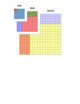
Figure 7: Band definition for 4x4, 8x8 and 16x16 blocks. The low frequencies are recursively divided following the pattern of smaller blocks. 4x4 blocks have all their AC coefficients in a single band.

6.1 Signaling

The last thing we need to discuss is how the parameters are transmitted from the encoder to the decoder. An important aspect of PVQ is to build activity masking into the codec, so that no extra information needs to be transmitted. We avoid explicitly signaling quantization resolution changes depending on the amount of contrast like other codecs currently do. Better, instead of only being able to signal activity masking rate changes at the macroblock level, we can do it at the block level and even per frequency band. We can treat horizontal coefficients independently of the vertical and diagonal ones, and do that separately for each octave.

Let’s start with the simplest case, where we do not have a predictor. The first parameter we code is the gain, which is raised to the power $(1-\alpha)$ when activity masking is enabled. From the gain alone, the bit-stream defines how to obtain $K$, so the decoder knows what $K$ is without the need to signal it. Once we know K, we can code the N-dimensional pyramid VQ codeword. Although it may look like we code more information than scalar quantization because we code the gain, it is not the case because knowing K makes it cheaper to code the remaining vector since we know the sum of the absolute values.

The case with prediction is only slightly more complicated. We still have to encode a gain, but this time we have a prediction, so we can use it to make coding the gain cheaper. After the gain, we code the angle $\theta$ with a resolution that depends on the gain. Last, we code a VQ codeword in $N-1$ dimensions. We only allow angles smaller than $\pi/2$, indicating a positive correlation with the predictor. To handle the cases where the input is poorly or negatively correlated with the predictor, we code a “no reference” flag. When set, we ignore the reference and only code the gain and an N-dimensional pyramid VQ codeword (no angle).

6.2 Coefficient Encoding

Encoding coefficients quantized with PVQ differs from encoding scalar-quantized coefficients since the sum of the coefficients’ magnitude is known (equal to $K$). While knowing $K$ places hard limits on the coefficient magnitudes that reduce the possible symbols that can be coded, much larger gains can be had by using it to improve probability modeling. It is possible to take advantage of the known $K$ value either through modeling the distribution of coefficient magnitudes or by modeling the length of zero runs. In the case of magnitude modeling, the expectation of the magnitude of coefficient $n$ is modeled as

$$E\left(\left|y_{n}\right|\right)=\mu\frac{K_{n}}{N-n}\ ,$$ (16)

where $K_{n}$ is the number of pulses left after encoding coefficients from $0$ to $n-1$ and $\mu$ depends on the distribution of the coefficients. For run-length modeling, the expectation of the position of the next non-zero coefficient is given by

$$E\left(run\right)=\nu\frac{N-n}{K_{n}}\ ,$$ (17)

where $\nu$ also models the coefficient distribution. Given the expectation, we code a value by assuming a Laplace distribution with that expectation. The parameters $\mu$ and $\nu$ are learned adaptively during the coding process, and we can switch between the two strategies based on $K_{n}$. Currently we start with magnitude modeling and switch to run-length modeling once $K_{n}$ drops to 1.

7 Results

The contrast masking algorithm is evaluated on both still a set of 50 still images taken from Wikipedia and downsampled to 1 megapixel, and on a set of short video clips ranging from CIF to 720p in resolution. First, the PSNR performance of scalar quantization vs. vector quantization is compared in Fig. 8a and 8c. To make comparison easier, we use a flat quantization matrix for both scalar and vector quantization.

Since we expect the use of contrast masking to make measurements such as PSNR worse, we evaluate its effect using a fast implementation of multi-scale structural similarity (FAST-SSIM) [10]. Fig. 8b and 8d show the FAST-SSIM results with and without contrast masking. For still images, the average improvement is 0.90 dB, equivalent to a 24.8% reduction in bitrate at equal quality, while for videos, the average improvement is 0.83 dB, equivalent to a 13.7% reduction in bitrate.

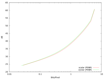
(a) Still image, PSNR of scalar vs vector quantization

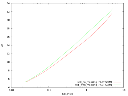
(b) Still image, FAST-SSIM with and without masking

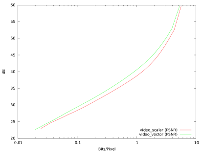
(c) Video, PSNR of scalar vs vector quantization

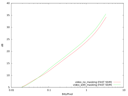
(d) Video, FAST-SSIM with and without masking

Figure 8: Comparing scalar quantization to vector quantization with and without contrast masking.

8 Conclusion

We have presented a perceptual vector quantization technique for still images and video. We have shown that it can be used to implement adaptive quantization based on contrast masking without any signaling in a way that improves quality. For now, contrast masking is restricted to the luma planes. It remains to be seen if a similar technique can be applied to the chroma planes.

This work is part of the Daala project [3]. The full source code, including all of the PVQ work described in this paper is available in the project git repository [11].

References

- [1] Osberger, W., [Perceptual Vision Models for Picture Quality Assessmnet and Compression Applications ], Queensland University of Technology, Brisbane (1999).
- [2] Valin, J.-M., Vos, K., and Terriberry, T. B., “Definition of the Opus Audio Codec.” RFC 6716 (Proposed Standard) (Sept. 2012).
- [3] “Daala website.” https://xiph.org/daala/.
- [4] Valin, J.-M., Maxwell, G., Terriberry, T. B., and Vos, K., “High-quality, low-delay music coding in the opus codec,” in [Proc. 135th AES Convention ], (Oct. 2013).
- [5] Lookabaugh, T. D. and Gray, R. M., “High-resolution quantization theory and the vector quantizer advantage,” IEEE Transactions on Information Theory 35, 1020–1033 (Sept. 1989).
- [6] Fischer, T. R., “A pyramid vector quantizer,” IEEE Trans. on Information Theory 32, 568–583 (1986).
- [7] Valin, J.-M., Terriberry, T. B., Montgomery, C., and Maxwell, G., “A high-quality speech and audio codec with less than 10 ms delay,” IEEE Trans. Audio, Speech and Language Processing 18(1), 58–67 (2010).
- [8] Johnston, J. D., “Transform coding of audio signals using perceptual noise criteria,” Selected Areas in Communications, IEEE Journal on 6(2), 314–323 (1988).
- [9] Fletcher, H. and Munson, W. A., “Relation between loudness and masking,” The Journal of the Acoustical Society of America 9(1), 78–78 (1937).
- [10] Chen, M.-J. and Bovik, A. C., “Fast structural similarity index algorithm,” in [Proc. ICASSP ], 994–997 (march 2010).
- [11] “Daala git repository.” https://git.xiph.org/daala.git.