Optimal Redshift Weighting For Redshift Space Distortions

Abstract

The low statistical errors on cosmological parameters promised by future galaxy surveys will only be realised with the development of new, fast, analysis methods that reduce potential systematic problems to low levels. We present an efficient method for measuring the evolution of the growth of structure using Redshift Space Distortions (RSD), that removes the need to make measurements in redshift shells. We provide sets of galaxy-weights that cover a wide range in redshift, but are optimised to provide differential information about cosmological evolution. These are derived to optimally measure the coefficients of a parameterisation of the redshift-dependent matter density, which provides a framework to measure deviations from the concordance $\Lambda$CDM cosmology, allowing for deviations in both geometric and/or growth. We test the robustness of the weights by comparing with alternative schemes and investigate the impact of galaxy bias. We extend the results to measure the combined anisotropic Baryon Acoustic Oscillation (BAO) and RSD signals.

1 Introduction

Forthcoming galaxy redshift surveys are motivated, to a large extent, by obtaining galaxy clustering measurements to accurately quantify the observed acceleration in the expansion of the Universe. It is to be hoped that these observations will reveal insight into the physical mechanism responsible for the cosmic acceleration, be it a new scalar field currently contributing to the energy budget of the Universe as Dark Energy, modification of gravitational laws on cosmological scales, or an unknown alternative to the Standard Cosmological Model.

Because the large-scale galaxy distribution is expected to follow a Gaussian random field, for which the statistical information is fully encoded in 2-point statistics, the central quantities in the analysis of galaxy surveys are the Correlation Function and its Fourier-space analogue, the Power Spectrum. The observed projections of these quantities encode significant cosmological information, including the positions of the Baryonic Acoustic Oscillations (BAO), which can be used as standard rulers to reconstruct the expansion history of the Universe, (Héctor Gil-Marín & SDSS-III Collaboration, 2016). The statistics also encode Redshift Space Distortions (RSD), which provide information about the large-scale growth of cosmological structure, (Hamilton, 1998).

The improvement in the statistical precision afforded by forthcoming surveys including DESI, (Levi et al., 2013) and Euclid, (Laureijs et al., 2011) are impressive, and will push at least an order of magnitude beyond current measurements. The improvement warrants a concerted effort to improve the methods used to analyse these data, and recent key developments include “reconstruction” to remove non-linear BAO damping, (Eisenstein et al., 2007), and the development of fast methods to measure the anisotropic clustering signal, (Bianchi et al., 2015; Scoccimarro, 2015).

One additional question to be answered is how best to combine future data from different volumes within the surveys, without losing information from galaxy pairs that span different bins, if using a binned approach and to optimally recover the desired signal. To deal with the first concern, we can make the transition from splitting into redshift-bins, to instead adopting weights that act to provide smoother windows on the data.

To optimise the weights, we must consider two factors: the first concerns changes in the observational efficiency as a function of position on the sky and redshift, and leads to weights that vary as a function of observed galaxy density, (Feldman et al., 1994), and bias , (Percival et al., 2004). The second concerns the cosmological models that we wish to distinguish between: Feldman et al. (1994), Percival et al. (2004) wished to optimally measure a power spectrum, which was assumed to be fixed within a survey volume. If instead, we wish to measure cosmological parameters that vary across a sample, for example a quantity that evolves with redshift, then the weights must additionally be optimised to measure this evolution.

In general, RSD measurements are made for a particular volume, presented as a single measurement at an effective redshift; if e.g. the growth factor varies in a non-linear way across the sample, the effective redshift is not a good approximation, by contrast by weighting the sample we allow for variation in redshift of all the measured quantities.

Zhu et al. (2015) presented weights optimised for measuring the distance-redshift relationship using the BAO signal. They considered a second-order expansion of the distance-redshift relationship around a fiducial cosmological model, and provided sets of weights for the monopole and quadrupole moments of the correlation function (or power spectrum) designed to optimally measure these parameters. In this paper we extend this derivation to the measurement of Redshift-Space Distortions, considering the weights required for these measurements, and how they compare to the BAO-optimised weights.

The outline of the paper is as follows. In Sec. 2 we briefly go through the method of linear data compression and we underline the advantages related. In Sec. 3 we present the cosmological model. In Sec. 4 we build to a derivation of the optimal weighting scheme for redshift space distortion measurements parametrized with respect to the matter energy density evolution in redshift, $\Omega_{m}(z)$. The choice of $\Omega_{m}$ parametrization allows to easily extend the results for more general clustering models which include both redshift space distortion and Alcock & Paczyński effects (1979), AP. In the second part of the section we compare them with other possible weights optimized for RSD measurements and we discuss our assumption for linear bias model. In Sec. 5 we derive the generalisation of optimal weights for RSD and AP test combined measurements. In Sec. 6 we discuss our results and present potential future improvements and applications.

2 Optimal Weights

The derivation of optimal weights is equivalent to the problem of optimal data compression: we use the weights to reduce the number of data points that need to be analysed to recover the cosmological parameters. We will now review how to optimally linearly compress our data, in the case of a covariance matrix known a priori, as described in Tegmark et al. (1997). Further details on the Karhunen-Loève methods in e.g. Vogeley & Szalay (1996) and Pope et al. (2004).

Given the $n$-dimensional data-set ${\bf x}$, assumed to be Gaussian distributed with mean ${\bf\mu}$ and covariance $C$, it can be linearly compressed into a new data-set $y$,

$$y=\textbf{w}^{T}\textbf{x},$$ (1)

where ${\bf w}$ is a $n$-dimensional vector of weights. The measurement $y$ has mean ${\bf w}^{T}{\bf\mu}$ and variance ${\bf w}^{T}C{\bf w}$.

The Fisher information matrix $F$ is defined as the second derivative of the logarithmic likelihood function $\mathcal{L}\equiv-\ln L$,

$$F_{ij}\equiv\left\langle\frac{\partial^{2}\mathcal{L}}{\partial\theta_{i}\partial\theta_{j}}\right\rangle,$$ (2)

for a set of parameters to be measured $\theta_{i}$. For a single parameter $\theta_{i}$,

$$F_{ii}=\frac{1}{2}\left(\frac{{\bf w}^{T}C_{,i}{\bf w}}{{\bf w}^{T}C{\bf w}}\right)^{2}+\frac{\left({\bf w}^{T}\mu_{,i}\right)^{2}}{{\bf w}^{T}C{\bf w}},$$ (3)

where the index $,i$ denotes $\partial/\partial\theta_{i}$. Note that the normalisation of the weights is arbitrary The search for optimal weights is equivalent to maximising $F_{ii}$ with respect to ${\bf w}$.

For a measurement of 2-point statistics from a galaxy survey, we should consider that ${\bf x}$ is the arrays formed by the measurements of the over-density squared, $\delta^{2}$ in configuration or Fourier space. Working in Fourier space, the covariance matrix $C$ of the power spectrum of the modes in the absence of a survey window is diagonal; for each redshift slice with volume $dV$ and expected galaxy density $\overline{n}(r)$,

$$C\sim\left(P_{\rm fid}+1/\overline{n}(r)\right)^{2}\dfrac{1}{dV},$$ (4)

where we have made the assumption that around the likelihood maxima, the power spectra $P_{fid}$ are drawn from a Gaussian distribution with fixed covariance matrix, e.g. Kalus et al. (2016). In this case, the first term in Eq. (3) vanishes. Maximising $F_{ii}$ with respect to ${\bf w}$, we find the only non-trivial eigenvector to be

$${\bf w}^{T}=C^{-1}{\bf\mu}_{,i},$$ (5)

and the new compressed data set reduces to

$$y={\bf\mu}_{,i}^{T}C^{-1}{\bf x}.$$ (6)

Note that, to linear order, $y$ contains the same information as ${\bf x}$, which can be checked by substituting ${\bf w}=C^{-1}{\bf\mu}_{,i}$ in Eq. (3), and seeing that $F$ remains unchanged. Eq. (5) forms the basis for our derivation of optimal weights.

Eq. (3) shows why it does not make sense to optimise for the set of $\delta$ (as opposed to $\delta^{2}$). This is because, although now the second term in Eq. (3) now vanishes as $\langle\delta\rangle=0$, the resulting eigenvector equation derived from the first term shows that there is no single set of optimal weights, even under the simplifying assumption of a diagonal covariance matrix. We can still apply the weights derived for $\delta^{2}$ to individual galaxies if we assume that the scales upon which clustering is being measured are small with respect to the cosmological changes that affect the relative weights. We would then simply weight each galaxy (and the expected density used to estimate $\delta$) by ${\bf w}_{\rm gal}=\sqrt{{\bf w}_{\delta^{2}}}$.

Note that the optimal set of weights given in Eq. (5) depends upon the derivatives of $\mu_{i}=P_{,i}$. Consequently in the rest of the paper we concentrate our analysis on the form of $P_{,i}$, which directly gives the form for the weights. If $P_{,i}$ matches for different measurements, then the optimal weights will also match.

The weights can be seen as a generalisation of the FKP weights presented in Feldman et al. (1994). The FKP weights are obtained by minimising the fractional variance in the power under the assumption that fluctuations are Gaussian and have the form

$$w_{\rm FKP}(r)=\frac{1}{1+\overline{n}(r)P(k)};$$ (7)

The weights defined by Eq. (5) depend on the inverse of the covariance matrix: assuming the redshift slices to be independent we can invert the Covariance matrix for a chosen scale and recover the FKP weights.

The cosmological model-dependent weights depend on the covariance matrix assumed and on the derivative of the mean value of the model with respect to the parameter that we want to estimate. Thus, once these quantities are fixed, it is not trivial to adapt a particular set of weights for different models. However, it would be very useful to set up weights that can be applied to make different measurements: both for computational reasons and in order to perform joint fits to the data. In this work we will start by deriving weights to be applied to RSD measurements and then we will broaden this to consider jointly measuring the RSD and the AP effect. Comparing the set of weights in these different situations shows whether it is likely that a single set of weights can be used to make optimal measurements in both situations.

3 Cosmological Model

3.1 Fiducial Cosmology

The $\Lambda$CDM scenario predicts the nature of dark energy as a cosmological constant with equation of state parameter $w=-1$ where the dynamical expansion of the Universe is specified by Friedmann equation

$$\frac{H_{\rm fid}^{2}(z)}{H_{0,fid}^{2}}=\Omega_{m,0,\rm fid}(1+z)^{3}+\Omega_{k,\rm fid}(1+z)^{2}+\Omega_{\Lambda,\rm fid}(z),$$ (8)

where the subscript the “$0$” stands for quantities evaluated at $z=0$ while “$\rm fid$” denotes fiducial quantities. With $\Omega_{\Lambda,\rm fid}$ dark energy density, $\Omega_{k,\rm fid}=1-\Omega_{m,\rm fid}-\Omega_{\Lambda,\rm fid}$ curvature, and $H_{0}$ the present-day Hubble parameter. We have

$$\Omega_{m,\rm fid}(z)=\frac{\Omega_{m,0,\rm fid}(1+z)^{3}}{H_{\rm fid}^{2}(z)/H^{2}_{0,\rm fid}},$$ (9)

where $\Omega_{m,0}$ refers to energy density evaluated at $z=0$. In a Friedmann-Roberston-Walker universe the solution for the linear growth factor $D_{\rm fid}(z)$ and the dimensionless linear growth rate $f$ are given by

$$\begin{split}g_{\rm fid}(\Omega_{m,\rm fid}(z))&\equiv\frac{D_{\rm fid}(z)}{a}\\ &=\frac{5\Omega_{m,\rm fid}(z)H_{\rm fid}^{3}(z)}{2(1+z)^{2}}\int_{z}^{\infty}\mathrm{d}z^{\prime}\frac{(1+z^{\prime})}{H_{\rm fid}^{3}(z^{\prime})}\end{split}$$ (10)

with scale factor $a$;

$$\begin{split}f_{\rm fid}(\Omega_{m,\rm fid}(z))=&-1-\frac{\Omega_{m,\rm fid}(z)}{2}+\Omega_{\Lambda,\rm fid}(z)\\ &+\frac{5\Omega_{m,\rm fid}(z)}{2g_{\rm fid}(z)}.\end{split}$$ (11)

Under the assumption of a flat universe i.e. $\Omega_{k,\rm fid}=0$, we have $\Omega_{\Lambda,\rm fid}(z)=1-\Omega_{m,\rm fid}(z)$.

For the fiducial galaxy bias model we choose a simple ad hoc functional form as used in Rassat et al. (2008), which is approximately correct for the $H\alpha$ galaxies to be observed by the Euclid survey,

$$b_{\rm fid}=\sqrt{1+z}.$$ (12)

3.2 Parametrising deviations

The derivation presented in Sec. 2 required us to define the parameters that we wish to optimise measurement of. We wish to choose parameters that allow us to measure deviations from the $\Lambda$CDM model. In the absence of compelling alternative cosmological models, we choose parameters that define an expansion in redshift of the cosmological behaviour we wish to understand - in our case the structure growth rate, and the expansion rate. Both of these can be modelled by deviations in $\Omega_{m}(z)$ away from the fiducial model, and we adopt this quantity as the redshift-evolving quantity that we wish to understand, rather than the distance-redshift relation considered by Zhu et al. (2015), which does not easily extend to structure growth differences. We expand $\Omega_{m}(z)$ around the fiducial model as,

$$\dfrac{\Omega_{m}(z)}{\Omega_{m,\rm fid}(z)}=q_{0}(1+q_{1}y(z)+\frac{1}{2}q_{2}y(z)^{2}),$$ (13)

we fix a pivot redshift $z_{p}$ within the survey redshift range and $y$ is defined as $y(z)+1\equiv\dfrac{\Omega_{m,\rm fid}(z)}{\Omega_{m,\rm fid}(z_{p})}$; the expansion parameters $q_{0}$, $q_{1}$, $q_{2}$ are obtained from Eq. 13 and its first and second derivatives evaluated at $z_{p}$;

$$\begin{split}q_{0}=&\dfrac{\Omega_{m}(z_{p})}{\Omega_{m,\rm fid}(z_{p})},\\ q_{1}=&\dfrac{\Omega_{m,\rm fid}(z_{p})}{\Omega_{m}(z_{p})}\dfrac{d\Omega_{m}/dz|_{z_{p}}}{d\Omega_{m,\rm fid}/dz|_{z_{p}}}-1,\\ q_{2}=&\bigg{[}\frac{\Omega_{m,\rm fid}(z_{p})}{\Omega_{m}(z_{p})}\frac{d^{2}\Omega_{m}}{dz^{2}}|_{z_{p}}-\frac{d^{2}\Omega_{m,\rm fid}}{dz^{2}}|_{z_{p}}\\ &-\left.\left(\dfrac{\Omega_{m,fid}(z_{p})}{\Omega_{m}(z_{p})}\dfrac{d\Omega_{m}/dz|_{z_{p}}}{d\Omega_{m,\rm fid}/dz|_{z_{p}}}-1\right)\left(\dfrac{2}{\Omega_{m,\rm fid}(z_{p})}\right.\right.\\ &\left(\frac{d\Omega_{m,\rm fid}}{dz}\right)^{2}|_{z_{p}}\left.+\frac{d^{2}\Omega_{m,\rm fid}}{dz^{2}}|_{z_{p}}\right)\bigg{]}\dfrac{\Omega_{m,\rm fid}(z_{p})}{\left(d\Omega_{m,\rm fid}/dz|_{z_{p}}\right)^{2}}.\end{split}$$ (14)

The Hubble parameter with respect to $\Omega_{m}(z)$ is

$$\frac{H^{2}(z)}{H^{2}_{0}}=\frac{\Omega_{m,0}(1+z)^{3}}{\Omega_{m}(z)},$$ (15)

where we have assumed that the dark matter equation of state is fixed,

$$\mathcal{P}=w\rho;\;w=0$$ (16)

with pressure $\mathcal{P}$ and matter density $\rho$.

A broader range of models could be derived by perturbing the homogeneous solution of the Einstein equations, but in this work we restrict ourselves to deviations close to $\Lambda\rm CDM$ in the dark energy and curvature components. The $\Omega_{m}$ parametrisation allows for many deviations from $\Lambda\rm CDM$: all the standard cosmological parameters can be written in terms of the $q_{i}$ parameters e.g. if we want to allow for modified gravity models we can parametrize the growth factor as a function of $\Omega_{m}(z)$. Alternatively, if we are studying the deviations from a fiducial geometry we can parametrize the AP parameters. We assume that Eqns. (10) & (11) hold for the perturbed $\Omega_{m}(z)$, which fix how the parameters $q_{i}$ lead to deviations in the growth rate away from the fiducial model.

4 Redshift weighting assuming known distance-redshift relation

In this section we derive a set of optimal weights to measure $\Omega_{m}(z)$ and the bias when the distance-redshift relation is assumed known, i.e we derive the weights for an observed power spectrum that contains only the distortion due to RSD and not due to AP effect.

We will discuss three different cases with different assumptions about parameters assumed known: the first two aim to estimate $\Omega_{m}(z)$ and the third the bias, parametrised by $b\sigma_{8}(z)$. In 4.2 we consider the case in which the bias is known and fixed to a fiducial model; in this case we are considering that the information about $\Omega_{m}$ is coming from all the terms of the Power Spectrum multipoles. We discuss this set of weight with respect to different fiducial models for the bias in order to test how knowing the bias would affect the results. However this first set of weights does not match the actual RSD measurements condition in which the bias is unknown. We then consider in 4.3 a case for RSD measurements where we assume the growth information is not coming from tangential power and the only information to be considered comes from $f\sigma_{8}$. Bias evolution plays an important role for clustering measurements even if, in the redshift range of interest for future and current surveys, $\Omega_{m}$ is significantly more sensitive to redshift than bias, (see Sec. 3). As our last case, in 4.4, we consider for completeness a set of weight to measure the bias relation as a function of redshift.

4.1 Modelling the observed power spectrum

For simplicity we adopt a linear model for the redshift-space distortions, assume that we are working in the plane parallel approximation, and assume a linear deterministic bias model so that the power spectrum in redshift space, $P^{s}$ is related to the real power spectrum $P$ by

$$P^{s}(\textbf{k})=(b+f\mu^{2}_{\textbf{k}})^{2}P(k)$$ (17)

where $P(k)$ is the linear real space power spectrum and where $\mu_{\textbf{k}}\equiv\hat{\textbf{z}}\cdot\hat{\textbf{k}}$ is the cosine of the angle between the wavevector k and the line of sight $\hat{\textbf{z}}$, (Kaiser, 1987).

It is common to decompose $P^{s}$ into an orthonormal basis of Legendre polynomials such that, in linear regime, the redshift power spectrum is well described by its first three non-null moments: monopole $P_{0}$, quadrupole $P_{2}$ and hexadecapole $P_{4}$.

$$P^{s}(\textbf{k})=\mathcal{P}_{0}(\mu_{\textbf{k}})P_{0}(k)+\mathcal{P}_{2}(\mu_{\textbf{k}})P_{2}(k)+\mathcal{P}_{4}(\mu_{\textbf{k}})P_{4}(k),$$ (18)

related with $P(k)$ through ,

$$P_{0}(k)=\left(b^{2}+\frac{2}{3}bf+\frac{1}{5}f^{2}\right)P(k)$$ (19)

,

$$P_{2}(k)=\left(\frac{4}{3}bf+\frac{4}{7}f^{2}\right)P(k),$$ (20)

$$P_{4}(k)=\left(\frac{8}{35}f^{2}\right)P(k).$$ (21)

We normalise the power spectrum using the standard variance of the galaxy distribution smoothed on scale $R=8h^{-1}$Mpc, $\sigma_{8}(z)$, where

$$\sigma_{8}(z)=\sigma_{8,0}D(z)=\sigma_{8,0}\frac{g(z)}{1+z}.$$ (22)

This normalisation enters into Eq. (17) in a way that is perfectly degenerate with $b$ and $f$, which could be replaced by new parameters $(b\sigma_{8})$ and $(f\sigma_{8})$.

4.2 Optimal weights to measure $\Omega_{m}(z)$ assuming known bias

We build optimal weights by taking the derivative of the power spectrum model with respect to the parameters $q_{i}$, As discussed in section 2, hereafter we only consider the component of these weights that varies with $P_{,i}$, which we denote for the monopole, quadrupole and hexadecapole, respectively $w_{0}$, $w_{2}$, $w_{4}$. For simplicity we refer to these as the “weights”, but it is worth remembering that there is a missing inverse variance component.

$$w_{\ell,q_{i}}=\dfrac{\partial P_{\ell}}{\partial q_{i}}$$ (23)

We explicitly write the redshift dependence of P on the $q_{i}$ parameters, so that the right side of Eq. (23) becomes

$$\dfrac{\partial P_{\ell}}{\partial q_{i}}=\dfrac{\partial P_{\ell}}{\partial f}\dfrac{\partial f}{\partial q_{i}}+\dfrac{\partial P_{\ell}}{\partial\sigma_{8}}\dfrac{\partial\sigma_{8}}{\partial q_{i}}$$ (24)

This second term assumes that we are recovering information from both radial and transverse modes. This is true for the transverse component if the bias is known perfectly. We build our set of weights as a function of redshift, for the monopole we have

$$w_{0,i}=\left(\frac{2}{3}b+\frac{2}{5}f\right)\sigma_{8}^{2}\frac{\partial f}{\partial q_{i}}+\left(b^{2}+\frac{2}{3}bf+\frac{1}{5}f^{2}\right)2\sigma_{8}\frac{\partial\sigma_{8}}{\partial q_{i}}$$ (25)

with

$$\frac{\partial f(z)}{q_{i}}=\frac{\partial\Omega_{m}(z)}{\partial q_{i}}\bigg{(}\frac{5}{2g(z)}-\frac{1}{2}\bigg{)}-\frac{\partial\Omega_{m}(z)}{\partial q_{i}}-\frac{5}{2}\frac{\Omega_{m}(z)}{g^{2}(z)}\frac{\partial g(z)}{\partial q_{i}},$$ (26)

$$\frac{\partial\sigma_{8}(z)}{\partial q_{i}}=\dfrac{\sigma_{8,0}}{1+z}\frac{\partial g(z)}{\partial q_{i}};$$ (27)

where

$$\begin{split}&\frac{\partial g(z)}{\partial q_{i}}=\frac{5}{2(1+z)^{2}}\bigg{(}\frac{\partial\Omega_{m}(z)}{\partial q_{i}}H^{3}(z)+3H^{2}(z)\frac{\partial H(z)}{\partial q_{i}}\Omega_{m}(z)\bigg{)}\cdot\\ &\int_{z}^{\infty}\mathrm{d}z^{\prime}\frac{(1+z^{\prime})}{H^{3}(z^{\prime})}-\frac{15\Omega_{m}(z)H^{3}(z)}{2(1+z)^{2}}\int_{z}^{\infty}\mathrm{d}z^{\prime}\frac{(1+z^{\prime})}{H^{4}(z^{\prime})}\frac{\partial H(z^{\prime})}{\partial q_{i}}\end{split}$$ (28)

$$\begin{split}\frac{\partial H(z)}{\partial q_{i}}=H_{0}\frac{1}{2}\left(\frac{\Omega_{m,0}(1+z)^{3}}{\Omega_{m}(z)}\right)^{-1/2}\frac{(1+z)^{3}}{\Omega_{m}(z)}\\ \cdot\left(\frac{\partial\Omega_{m,0}}{\partial q_{i}}-\frac{\Omega_{m,0}}{\Omega_{m}}\frac{\partial\Omega_{m}(z)}{\partial q_{i}}\right),\end{split}$$ (29)

with

$$\begin{split}\frac{\partial\Omega_{m}}{\partial q_{0}}&=\Omega_{m,fid}(z),\\ \frac{\partial\Omega_{m}}{\partial q_{1}}&=\Omega_{m,\rm fid}(z)y(z),\\ \frac{\partial\Omega_{m}}{\partial q_{2}}&=\Omega_{m,\rm fid}(z)\frac{y^{2}(z)}{2}.\\ \end{split}$$ (30)

Note that in the equations above the $P(k)$ term has been factored out; all the terms are evaluated at $q_{0}=1$ since we are ignoring the weights dependence on cosmology.

Similarly for the quadrupole and for the hexadecapole

$$\begin{split}w_{2,q_{i}}&=\left(\frac{4}{3}b+\frac{8}{7}f\right)\sigma_{8}^{2}\frac{\partial f}{\partial q_{i}}+\left(\frac{4}{3}bf+\frac{4}{7}f^{2}\right)2\sigma_{8}\frac{\partial\sigma_{8}}{\partial q_{i}},\\ &\\ w_{4,i}&=\frac{16}{35}f\sigma_{8}^{2}\frac{\partial f}{\partial q_{i}}+\frac{8}{35}f^{2}2\sigma_{8}\frac{\partial\sigma_{8}}{\partial q_{i}}.\end{split}$$ (31)

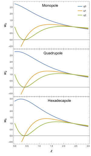
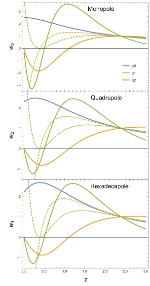
Figure 1 shows the set of weights for the monopole, quadrupole and hexadecapole, with a convenient normalization. All the plot are generated considering a $\Lambda$CDM model with $\Omega_{m,0}=0.31$ as the fiducial cosmology. We explore a wide redshift range to see general trends, as if we are analysing data from a range of surveys. We fix a pivot redshift in $z_{p}=0.4$. All three weights with respect to parameters $q_{0}$ (blue lines) show a peak at redshift $z\sim 0.1-0.2$; this is due to $\partial\Omega_{m}/\partial q_{i}$ term which rapidly grows until about $z\sim 2$ and then tends to a constant. The peak corresponds to the $\Omega_{m}\sim\Omega_{\Lambda}$ epoch: the weights aim to highlight the deviations from the fiducial cosmology $\Lambda\rm CDM$, and therefore peak approximately in the range of the equivalence between matter and $\Lambda$. At higher redshifts the weights decrease due to the decreasing dependence of $\Omega_{m}(z)$ on $f$ and $\sigma_{8}$.

The weights about the slope parameters, $q_{1}$ (orange line), rapidly grow at low redshift driven by $\partial\Omega_{m}/\partial q_{1}$ and $\partial P_{\ell}/\partial\sigma_{8}$, and then start decreasing as $\partial f/\partial\Omega_{m}$ and $\partial P_{\ell}/\Omega_{m}$ dominate. We see that they pickup small differences about the peak due to the different dependencies on $P_{\ell}$.

The green lines displays the weights with respect to the second order parameter $q_{2}$: they are similar, with a minimum about $z$ $\sim 0.5$: this difference with respect to $q_{0}$ and $q_{1}$ is due to the $\partial\Omega_{m}/\partial q_{2}$ term, which starts decreasing with $z$ until about $z\sim 0.4$ and then slowly increases. Comparing the monopole, quadrupole and hexadecapole weights we see that the weights behave in a similar way for all three statistics; the hexadecapole weights show a faster decrease for all three parameters, due to the absence of the bias dependence. However the differences with monopole and quadrupole are small, confirming our assumption that the bias choice does not drastically change the weights in the region of interest.

Figure 1: The weights for the monopole ($w_{0}$) , quadrupole ($w_{2}$) and hexadecapole ($w_{4}$) with respect to the $q_{i}$ parameters: blue lines indicate the weight with respect to $q_{0}$, orange lines indicate the weight with respect to $q_{1}$ and the green lines the weight with respect to $q_{2}$. These weights assume a fiducial bias evolving as $b=\sqrt{1+z}$ and were calculated for RSD measurements assuming that the bias is known, as described in Sec. 4.2.

4.2.1 Application of the method

We have derived a set of weights that compress the information available in the power spectrum across a range of redshifts. In practice, to apply the method, we weight galaxies, assuming ${\bf w}_{\rm gal}=\sqrt{{\bf w}_{\delta^{2}}}$, to obtain a set of monopole, quadrupole and hexadecapole for each set of weights.

If we were only interested in a single parameter, (e.g. $q_{0}$) and we thought all the information came from the monopole, we would measure the weighted $P_{w,0}$ by applying the $w_{0,q_{0}}$ to each galaxy; we would then fit $q_{0}$ by comparing the data with the theoretical prediction for the monopole, weighted at different redshifts as

$$P_{0,w_{0,q_{0}}\rm model}(k)=\int dz\;P_{0}(k,z)\cdot w_{0,q_{0}}(z).$$ (32)

Where the $P_{0}(k,z,q_{0})$ corresponds to the monopole prediction, e.g Eq.19 and we have ignored the window effects. If we further assume the simple linear model for RSD, (Kaiser, 1987),

$$P_{0}(k,z)=\left(b^{2}+\frac{2}{3}bf(\Omega_{m}(q_{0},z))+\frac{1}{5}f(\Omega_{m}(q_{0},z))^{2}\right)P(k);$$ (33)

we can express $f$ in terms of $\Omega_{m}(q_{0},z)$ according to Eq. 11.

In order to simultaneously measure all three $q_{i}$ parameters, we measure each multipole weighted to be optimal for each $q_{i}$ parameters, i.e. we weight galaxies with the different $w_{i,q_{j}}$ functions and we build a data vector $\Pi$ as,

$$\Pi^{T}=(P_{0,w_{0},q_{0}},P_{0,w_{0},q_{1}},P_{0,w_{0},q_{2}}\;...\;P_{4,w_{4},q_{2}})^{\rm T}.$$ (34)

Note that each weighted multipole $P_{i,w_{i,q_{j}}}$ provides a particular piece of information about $\Omega_{m}(z)$ that optimizes the measurement of each $q_{i}$. We constrain the three $q_{i}$ by jointly fitting from the data-vector $\Pi$ compared with a $\Pi_{\rm model}$. In practice we assume a Gaussian likelihood and minimize

$$\chi^{2}\propto(\Pi-\Pi_{\rm model})^{\rm T}C^{-1}(\Pi-\Pi_{\rm model});$$ (35)

where each $P_{i,w_{i,q_{j}}}$ inside $\Pi_{\rm model}$ is modeled as in Eq. 32. The $C^{-1}$ term corresponds to the joint covariance matrix.

4.2.2 The dependence on the fiducial bias model

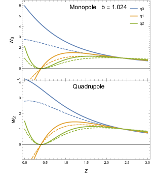
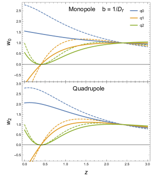
We now test the robustness of the set of weights for $\Omega_{m}$, presented in 4.2, with respect to the bias model. To do this we compute sets of weights from different choices of $b(z)$. We first derive the set of weights presented in Sec. 4, parametrized with respect to $\Omega_{m}$, fixing a constant bias, $b=1.024$, which is our fiducial value at $z=0.45$, then we repeat for $b=1/D_{\rm fid}(z)$.

Figures 2, 3 show that the behaviour of the weights with redshift is similar to previous results and there are no significant differences in the shapes. As expected the differences are more visible in the monopole (top panel) than in the quadrupole (bottom panel) since the former is more sensitive to galaxy bias. We exclude the weights for the hexadecapole since it does not depend on galaxy bias.

Figure 2: Solid lines as Fig. 1, but assuming a constant bias $b=1.024$. We compare this set of weights with the results presented in Fig 1, (dashed lines), obtained assuming a bias evolving as $b=\sqrt{1+z}$.

Figure 3: Solid lines as Fig. 1, but assuming a fiducial bias evolving with redshift as $b=1/D_{f}(z)$. We compare this set of weights with the results presented in Fig 1, (dashed lines), obtained assuming a bias evolving as $b=\sqrt{1+z}$.

4.3 Optimal weights to measure $\Omega_{m}(z)$ with unknown bias

RSD measurements constrain the product of the two key parameters $f$ and $\sigma_{8}$ and it is common to consider a single measurement of $[f\sigma_{8}]$, marginalising over an unknown bias. Therefore we present a set of weights that matches the philosophy of current RSD measurements: we consider the term $[b\sigma_{8}]$ to be independent from $[f\sigma_{8}]$ since we marginalize over the bias. Considering e.g. the monopole

$$P_{0}=\bigg{(}[b\sigma_{8}]^{2}+\frac{2}{3}[b\sigma_{8}][f\sigma_{8}](z)+\frac{1}{5}[f\sigma_{8}]^{2}(z)\bigg{)}P(k)/(\sigma_{8}^{2})$$ (36)

for unknown bias the dependence on the $q_{i}$ parameters is only through $[f\sigma_{8}]$. We derive the set of weight by taking the derivative of $P_{0}$, $P_{2}$, $P_{4}$ with respect to $q_{1}$, $q_{2}$, $q_{3}$,

$$w_{0,q_{i}}\equiv\left(\frac{2}{3}[b\sigma_{8}]+\frac{2}{5}[f\sigma_{8}](z)\right)\frac{\partial[f\sigma_{8}]}{\partial q_{i}}(z),$$ (37)

$$w_{2,q_{i}}\equiv\left(\frac{4}{3}[b\sigma_{8}]+\frac{8}{7}[f\sigma_{8}](z)\right)\frac{\partial[f\sigma_{8}]}{\partial q_{i}}(z),$$ (38)

$$w_{4,q_{i}}\equiv\left(\frac{16}{35}[f\sigma_{8}](z)\right)\frac{\partial[f\sigma_{8}]}{\partial q_{i}}(z),$$ (39)

where the derivatives $\partial[f\sigma_{8}]/\partial q_{i}(z)$ are obtained using Eq. 26 and 27.

Figure 4: Solid lines show weights for the monopole ($w_{0}$) quadrupole ($w_{2}$) and hexadecapole ($w_{4}$) , with respect to the $q_{i}$ parameters ignoring the information in $b\sigma_{8}$ term, as described in Sec. 4.3. These are compared with the weights presented in Fig. 1 (dashed lines), which assume the bias is known.

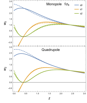
Figure 4, shows the set of weights for the monopole, quadrupole and hexadecapole parametrized with respect to $q_{0}$, $q_{1}$, $q_{2}$, when ignoring the information contained in $[b\sigma_{8}]$, conveniently normalised. We compare them with the weights derived in 4.2, presented in Fig 1, (dashed lines). The main difference between the two set of weights lies on the assumptions we make for galaxy bias: if we are setting it as completely unknown, considering only the information contained in $[f\sigma_{8}]$ or if we are including $[b\sigma_{8}]$ term, constraining $b(z)$ to a fiducial model; however the plots show a very similar behaviour between the two cases, it is clear then that the tangential modes do not play a large role in determining optimal weights.

4.4 Optimal weights to measure bias

For completeness we will show how to derive weights that optimally measure the evolution of the bias parameter around the fiducial model.

In an analogous manner to Eq. 13 we model $[b\sigma_{8}](z)$ as an expansion about a fiducial model $[b\sigma_{8}]_{\rm fid}$:

$$\dfrac{[b\sigma_{8}](z)}{[b\sigma_{8}]_{\rm fid}(z)}=\eta_{0}\left(1+\eta_{1}x+\dfrac{1}{2}\eta_{2}x^{2}\right)$$ (40)

about a pivot redshift $z_{p}$, where $1+x\equiv\frac{[b\sigma_{8}]_{\rm fid}(z)}{[b\sigma_{8}]_{\rm fid}(z_{p})}$.

The $\eta$ parameters correspond to the derivative 0,1,2 of $[b\sigma_{8}](z)$ relation evaluated at $z_{p}$.

In analogy with measuring $q_{i}$, we can derive a set of weights that optimally estimate the bias-redshift through the $\eta_{j}$ parameters,

$$w_{\ell,\eta_{j}}=\frac{\partial P_{\ell}}{\partial[b\sigma_{8}]}\frac{\partial[b\sigma_{8}]}{\eta_{j}}$$ (41)

This set of weights can be applied instead of the set of weights with respect to $\Omega_{m}$ in case we want to measure deviations from the fiducial model chosen for the bias. We do not plot these weights for simplicity but include the derivation to show how they could be calculated.

5 Redshift weighting assuming unknown distance-redshift relation

Our previous results provide an optimal scheme specific for RSD measurements; as pointed out in the introduction it would be very useful to optimize at the same time geometric measurements and thus enable measurements that include all the parameters both for computational costs either for accuracy of the results. An optimal weighted scheme for BAO measurements has been recently presented in Zhu et al. (2015) where the authors describe a weighting scheme parametrized with respect to the distance-redshift relation, including the AP effect modelled as

$$\begin{split}k_{\perp}&\rightarrow\alpha^{-1}(1+\epsilon)k_{\perp},\\ k_{\parallel}&\rightarrow\alpha^{-1}(1+\epsilon)^{-2}k_{\parallel},\end{split}$$ (42)

with parameters $\alpha$, for isotropic deformation and $\epsilon$, for anisotropic. The method optimises only BAO measurements, constraining the covariance matrix at BAO scales and ignoring the growth parameters.

In this section we will account for both distortions due to peculiar velocities and distortions due to incorrect choice of geometry described by Alcock-Paczyński effect. We still use a parametrization of $\Omega_{m}(z)$ to define deviations from our fiducial model as described in Eq. 13.

5.1 Modelling AP and RSD in the observed $P(k)$

We denote $k^{t}$ and $k$ the true and observed coordinates respectively, then assuming an incorrect geometry transforms the coordinates

$$\begin{split}k^{t}&=\frac{k}{\alpha_{\perp}}\left[1+\mu^{2}\left(\frac{\alpha_{\perp}^{2}}{\alpha_{\parallel}^{2}}-1\right)\right]^{1/2},\\ \mu^{t}&=\mu\frac{\alpha_{\perp}}{\alpha_{\parallel}}\left[1+\mu^{2}\left(\frac{\alpha_{\perp}^{2}}{\alpha_{\parallel}^{2}}-1\right)\right]^{-1/2},\end{split}$$ (43)

with $\alpha_{\parallel}$ defined as the ratio between the observed and the true Hubble parameter, $H(z)/H_{t}(z)$ and $\alpha_{\perp}$ defined as ratio between the true and the observed angular diameter distance $D_{A,t}(z)$ / $D_{A}(z)$, e.g. (Ballinger et al., 1996); the multipoles at the observed $k$ are related to the Power Spectrum at $k^{t}$, through

$$P_{\ell}(k)=\frac{2\ell+1}{2}\int_{-1}^{1}d\mu P(k^{t},\mu^{t})\mathcal{L}_{\ell}(\mu)$$ (44)

For linear redshift space distortion, Kaiser (1987), inserting the transformation of the coordinates given by Eq. 43, the galaxy power spectrum at the true wavenumber is

$$\begin{split}P^{s}(k^{t},\mu^{t})=\dfrac{1}{\alpha_{\perp}^{2}\alpha_{\parallel}}P\left[\frac{k}{\alpha_{\perp}}\left[1+\mu^{2}\left(\frac{\alpha_{\perp}^{2}}{\alpha_{\parallel}^{2}}-1\right)\right]^{1/2}\right]&\\ \left[1+\mu^{2}\left(\frac{\alpha_{\perp}^{2}}{\alpha_{\parallel}^{2}}-1\right)\right]^{-2}\left\{1+\mu^{2}\left[(\beta+1)\frac{\alpha_{\perp}^{2}}{\alpha_{\parallel}^{2}}-1\right]\right\}^{2}&.\end{split}$$ (45)

We use the notation $\beta\equiv f/b$ for simplicity with equations. We expand at first order $P$ in the right side of Eq. 45, in order to get analytical derivatives with respect to the expansion parameters. We have tested numerically that this approximation does not influence our conclusions. Introducing $\varphi\equiv\frac{\alpha_{\perp}^{2}}{\alpha_{\parallel}^{2}}-1$, we can expand the right side of Eq. 45 to first order about $(\alpha_{\perp},\varphi)=(1,0)$, using

$$\begin{split}&P\left[\frac{k}{\alpha_{\perp}}\left(1+\mu^{2}\varphi\right)^{1/2}\right]\approx P(k)+\\ &(\alpha_{\perp}-1)\left.\dfrac{\partial P}{\partial k}\dfrac{\partial k}{\partial k^{t}}\dfrac{\partial k^{t}}{\partial\alpha_{\perp}}\right|_{\begin{subarray}{c}{\alpha_{\perp}=1}\\ {\;\;\;\varphi=0}\end{subarray}}+\varphi\left.\dfrac{\partial P}{\partial k}\dfrac{\partial k}{\partial k^{t}}\dfrac{\partial k^{t}}{\partial\varphi}\right|_{\begin{subarray}{c}{\alpha_{\perp}=1}\\ {\;\;\;\varphi=0}\end{subarray}}\end{split}$$ (46)

Substituting in Eq. 45 and then in Eq. 44, we obtain models of the multipoles accounting for both RSD and AP effects to be

$$\begin{split}&P_{\ell}(k)=\dfrac{2\ell+1}{2}\int_{-1}^{1}d\mu\mathcal{L}_{\ell}(\mu)\left\{P(k)\left(1+\mu^{2}\beta\right)^{2}+\right.\\ &\varphi\left[\dfrac{1}{2}\dfrac{\partial P}{\partial\ln k}\mu^{2}\left(1+\mu^{2}\beta\right)^{2}+P(k)(-2\mu^{2})(1+\beta\mu^{2})^{2}+\right.\\ &\left.2\mu^{2}(1+\beta\mu^{2})(1+\beta)P(k)-\dfrac{1}{2}P(k)(1+\mu^{2}\beta)^{2}\right]+\\ &\left.(1-\alpha_{\perp})(1+\mu^{2}\beta)^{2}\left(\frac{\partial P}{\partial\ln k}+3P(k)\right)\right\}\end{split}$$ (47)

In particular it holds that $P^{s}(k)$ at linear order is described by the first three multipoles, Ross & et al. (2015). The monopole, quadrupole and hexadecapole are

$$\begin{split}P_{0}(k)&=\dfrac{1}{2}\sigma_{8}^{2}\bigg{\{}\left(2+\dfrac{4}{3}\beta+\dfrac{2}{5}\beta^{2}\right)P(k)+\varphi\bigg{[}\bigg{(}\dfrac{1}{3}+\dfrac{2}{5}\beta+\dfrac{1}{7}\beta^{2}\bigg{)}\\ &\dfrac{\partial P}{\partial\ln k}-\left(1+\dfrac{2}{15}\beta-\dfrac{1}{35}\beta^{2}\right)P(k)\bigg{]}+(1-\alpha_{\perp})\bigg{(}2\\ &+\dfrac{4}{3}\beta+\dfrac{2}{5}\beta^{2}\bigg{)}\left(\frac{\partial P}{\partial\ln k}+3P(k)\right)\bigg{\}},\\ P_{2}(k)&=\dfrac{5}{2}\sigma_{8}^{2}\bigg{\{}\bigg{(}\dfrac{8}{15}\beta+\dfrac{8}{35}\beta^{2}\bigg{)}P(k)+\varphi\bigg{[}\bigg{(}\dfrac{2}{15}+\dfrac{8}{35}\beta\\ &+\dfrac{2}{21}\beta^{2}\bigg{)}\dfrac{\partial P}{\partial\ln k}-\left.\left(\dfrac{4}{21}\beta+\dfrac{4}{105}\beta^{2}\right)P(k)\right]+(1-\\ &\alpha_{\perp})\left(\dfrac{8}{15}\beta+\dfrac{8}{35}\beta^{2}\right)\left.\left(\frac{\partial P}{\partial\ln k}+3P(k)\right)\right\},\\ P_{4}(k)&=\dfrac{9}{2}\sigma_{8}^{2}\bigg{\{}\dfrac{16}{315}\beta^{2}P(k)+\varphi\left[\left(\dfrac{16}{315}\beta+\dfrac{8}{231}\beta^{2}\right)\dfrac{\partial P}{\partial\ln k}\right.\\ &-\left.\left(\dfrac{32}{315}\beta+\dfrac{24}{385}\beta^{2}\right)P(k)\right]+(1-\alpha_{\perp})\dfrac{16}{315}\beta^{2}\bigg{(}\frac{\partial P}{\partial\ln k}+\\ &3P(k)\bigg{)}\bigg{\}}.\end{split}$$ (48)

5.2 AP and RSD weights derivation, assuming known bias

As before, the weights for the power spectrum multipoles, assuming information from both RSD and AP effects, are obtained by taking the derivative of the $P_{i}$ with respect to the $q_{i}$ parameters defined in 3.2,

$$\begin{split}w_{\ell,q_{i}}=\dfrac{\partial P_{\ell}}{\partial q_{i}}&=\frac{\partial P_{\ell}}{\partial\varphi}\frac{\partial\varphi}{\partial q_{i}}+\frac{\partial P_{\ell}}{\partial\alpha_{\perp}}\frac{\partial\alpha_{\perp}}{\partial q_{i}}\\ &+\frac{\partial P_{\ell}}{\partial\beta}\frac{\partial\beta}{\partial f}\frac{\partial f}{\partial q_{i}}+\frac{\partial P_{\ell}}{\partial\sigma_{8}}\frac{\partial\sigma_{8}}{\partial q_{i}}.\end{split}$$ (49)

all the derivatives are evaluated at the fiducial model. In case of flat universe we have

$$\alpha_{\perp}(z)=\frac{\int^{z}_{0}\mathrm{d}z^{\prime}1/H(q_{i},z^{\prime})}{\int^{z}_{0}\mathrm{d}z^{\prime\prime}1/H_{\rm fid}(z^{\prime\prime})}$$ (50)

Inserting the definition of $\beta$ and $\varphi$,

$$\begin{split}&\frac{\partial\beta}{\partial f}=\frac{1}{b},\\ &\dfrac{\partial\varphi}{\partial q_{i}}=-\dfrac{2\alpha_{\perp}^{3}}{\alpha_{\parallel}^{3}}\bigg{(}\frac{1}{\alpha_{\perp}}\frac{\partial\alpha_{\parallel}}{\partial q_{i}}+\frac{-\alpha_{\parallel}}{\alpha^{2}_{\perp}}\frac{\partial\alpha_{\perp}}{\partial q_{i}}\bigg{)},\\ \end{split}$$ (51)

where

$$\begin{split}\frac{\partial\alpha_{\parallel}}{\partial q_{i}}&=-\frac{1}{H_{\rm fid}(z)}\frac{\partial H}{\partial q_{i}},\\ \frac{\partial\alpha_{\perp}}{\partial q_{i}}&==\frac{\int^{z}_{0}\mathrm{d}z^{\prime}-\frac{1}{H_{\rm fid}^{2}(z^{\prime})}\frac{\partial H}{\partial q_{i}}}{\int^{z}_{0}\mathrm{d}z^{\prime\prime}1/H_{\rm fid}(z^{\prime\prime})}.\\ \end{split}$$ (52)

In Appendix References we present the derivatives of the multipoles $P_{i}$ with respect to $\varphi$, $\alpha_{\perp}$, $f$ and $\sigma_{8}$.

The weights have arbitrary normalization but we cannot factor out the scale dependence as we did for the RSD weights since we now have two different $k$-dependent terms $P$ and $dP/d\ln k$. However Zhao et al. (2015) show that this dependence is very weak.

Figure 5 shows the weights optimal for RSD and AP measurements evaluated at $k=0.1$ $h\;\rm MPc^{-1}$, for the monopole, quadrupole and hexadecapole respectively. Blue lines indicate the weights with respect to $q_{0}$, orange lines with respect to $q_{1}$ and green lines with respect to $q_{2}$. Comparing with the previous result that assumed a known distance-redshift relation (dashed lines), it is possible to see that the behaviour of the three weights does not change drastically. In general the redshift dependence is stronger including also the AP effect and the new weights show a more enhanced maximum. Since the contribution from $\varphi$ and $\alpha_{\perp}$ vanish for $q_{0}$, the weights $w_{i,q_{0}}$ are equivalent to the previous weights without AP effect. (Fig 1).

5.3 AP-RSD weights assuming unknown bias

If we now neglect the information given by $[b\sigma_{8}]$, as we did for one set of RSD weights, we substitute $\beta=f/b$, then we change the Eq. LABEL:cool to

$$\begin{split}w_{\ell,q_{i}}=\dfrac{\partial P_{\ell}}{\partial q_{i}}&=\frac{\partial P_{\ell}}{\partial\varphi}\frac{\partial\varphi}{\partial_{i}}+\frac{\partial P_{\ell}}{\partial\alpha_{\perp}}\frac{\partial\alpha_{\perp}}{\partial q_{i}}\\ &+\frac{\partial P_{\ell}}{\partial f\sigma_{8}}\frac{\partial f\sigma_{8}}{\partial q_{i}},\end{split}$$ (53)

where we have assumed that $\partial[b\sigma_{8}]/\partial q_{i}=0$.

In Sec 4 we showed that there are no significant differences between the cases in which $b\sigma_{8}$ is known and unknown, however, for the reasons discussed in Sec. 4, they are more consistent with the RSD measurements. We do not plot any new results since the differences are very small.

Figure 5: The RSD + AP optimal weights for the monopole $w_{0}$, quadrupole $w_{2}$, hexadecapole $w_{4}$. Blue lines indicate the weights with respect to the $q_{0}$ parameter. Orange lines indicate the weights with respect to the $q_{1}$ parameter and green lines indicates the weights with respect to the $q_{2}$ parameter. We compare them with previous results, where the distance-redshift relation was fixed (dashed lines); the weights $w_{\ell,q_{0}}$ (blue lines) are equivalent to the previous weights without AP effect since the contribute from $\varphi$ and $\alpha_{\perp}$ vanish because of $\partial H(q_{i})/\partial q_{0}=0$. The RSD+AP weights show enhanced features due to AP parameters, whose importance increases with redshift.

6 Discussion

In the first part of the paper we presented a set of optimal redshift dependent weights for RSD measurements. These functions allow us to optimally compress the original dataset while minimising the error a priori provided by the Fisher matrix, on the parameters we want to measure. In contrast to current RSD measurements, which compare the data with the model at a single effective redshift, the weights presented account for the redshift evolution of the cosmological effects, since the measurements are now compared with a weighted model covering a range of redshifts. The method is based on a particular choice of a relation in redshift we want to measure/investigate, e.g modelled as an expansion about a fiducial model. We derived the set of weights that optimally estimates deviations from a $\Lambda CDM$ background, modelled using variations of $\Omega_{m}(z)$; we modelled $\Omega_{m}(z)$ as a polynomial expansion in terms of parameters $q_{i}$ about a fixed fiducial models $\Omega_{m,\rm fid}$, then we applied the compression method as described in Tegmark et al. (1997) and derived the set of weights that optimally estimates the expansion parameters. As explained in section 2, our weights generalise the FKP weights: they take in account of the galaxy density distribution through the Covariance Matrix and allow sensitivity to the redshift dependence of the statistics we are measuring.

We started assuming a known distance-redshift relation and considering two different cases: one in which the bias is known and constrained to a fiducial model and one in which the bias is unknown and we marginalize over it. We compared them and we showed the consistency between the two scheme: this means that the bias does not play a large role in determining the weights. We also tested our assumptions on the fiducial bias model by deriving the previous results for two different bias models. We confirmed also in this case that the weights are not significantly sensitive to $b(z)$. For completeness we presented a further set of weights that optimize the measurement of bias.

In order to improve future measurements we extended the previous weights to a more general case, when the distance-redshift relation is unknown: we modelled the observed power spectrum including the AP effect; we introduced two new distortion parameters $\varphi$, $\alpha_{\perp}$ in $P(k)$ describing the AP effect. The set of weights obtained for RSD and AP measurements is scale dependent through the ratio of $P(k)$ and its logarithmic derivative. This is not a particular issue for future applications since this dependence is predicted to be very weak, moreover considering e.g. Camb, (Lewis & Bridle, 2002), computing $P(k)$ model in real space or its derivative will not require high computational time, provided we apply these weights after calculating the power. Zhu et al. did not face with this problem since they constrained every quantity on the BAO scale (k $\sim$ $0.1hMpc^{-1}$ ). We compared the new results with the weights accounting for RSD only at BAO scale showing that the redshift dependence is now increased by the inclusion of the AP parameters.

In order to correctly apply the weighting scheme we will need to understand how to combine with weights designed to correct for systematic density field distortions. The derivations presented made a number of assumptions (e.g the fact that the Power Spectrum shape is equal for each redshift slice and that $P$ is Gaussian distributed). It would be interesting to see if the weights change when we relax these assumptions -we leave this for future work.

Appendix A Derivative of the multipoles with respect to $\varphi$, $\alpha_{\perp}$, $\beta$, $\sigma_{8}$.

We here present the derivatives of the generalised multipoles computed in Sec. 5.1, with respect to the redshift dependent parameters.

$$\begin{split}\frac{\partial P_{0}}{\partial\varphi}=&\frac{1}{2}\sigma_{8}^{2}\bigg{[}\bigg{(}\frac{1}{3}+\frac{2}{5}\beta+\frac{1}{7}\beta^{2}\bigg{)}\frac{\partial P}{\partial\ln k}-\bigg{(}1+\dfrac{2}{15}\beta-\\ &\dfrac{1}{35}\beta^{2}\bigg{)}P(k)\bigg{]}\\ \frac{\partial P_{0}}{\partial\alpha_{\perp}}=&-\frac{1}{2}\sigma_{8}^{2}\bigg{(}2+\dfrac{4}{3}\beta+\dfrac{2}{5}\beta^{2}\bigg{)}\bigg{(}\frac{\partial P}{\partial\ln k}+3P(k)\bigg{)}\\ \frac{\partial P_{0}}{\partial\beta}=&\frac{1}{2}\sigma_{8}^{2}\bigg{\{}\bigg{(}\frac{4}{3}+\frac{4}{5}\beta\bigg{)}P(k)\\ \frac{\partial P_{0}}{\partial\sigma_{8}}=&\sigma_{8}\bigg{(}2+\dfrac{4}{3}\beta+\dfrac{2}{5}\beta^{2}\bigg{)}P(k)\end{split}$$ (54)

$$\begin{split}\frac{\partial P_{2}}{\partial\varphi}=&\frac{5}{2}\sigma_{8}^{2}\bigg{[}\bigg{(}\dfrac{2}{15}+\dfrac{8}{35}\beta+\dfrac{2}{21}\beta^{2}\bigg{)}\dfrac{\partial P}{\partial\ln k}-\bigg{(}\dfrac{4}{21}\beta+\dfrac{4}{105}\beta^{2}\\ &\bigg{)}P(k)\bigg{]}\\ \frac{\partial P_{2}}{\partial\alpha_{\perp}}=&-\frac{5}{2}\sigma_{8}^{2}\bigg{(}\dfrac{8}{15}\beta+\dfrac{8}{35}\beta^{2}\bigg{)}\bigg{(}\frac{\partial P}{\partial\ln k}+3P(k)\bigg{)}\\ \frac{\partial P_{2}}{\partial\beta}=&\frac{5}{2}\sigma_{8}^{2}\bigg{(}\frac{8}{15}+\frac{16}{35}\beta\bigg{)}P(k)\\ \frac{\partial P_{2}}{\partial\sigma_{8}}=&5\sigma_{8}\bigg{(}\dfrac{8}{15}\beta+\dfrac{8}{35}\beta^{2}\bigg{)}P(k)\end{split}$$ (55)

$$\begin{split}\frac{\partial P_{4}}{\partial\varphi}=&\dfrac{9}{2}\sigma_{8}^{2}\bigg{[}\left(\dfrac{16}{315}\beta+\dfrac{8}{231}\beta^{2}\right)\dfrac{\partial P}{\partial\ln k}-\left(\dfrac{32}{315}\beta+\dfrac{24}{385}\beta^{2}\right)\\ P(k)\bigg{]}\\ \frac{\partial P_{4}}{\partial\alpha_{\perp}}=&-\dfrac{9}{2}\sigma_{8}^{2}\bigg{\{}\dfrac{16}{315}\beta^{2}\bigg{(}\frac{\partial P}{\partial\ln k}+3P(k)\bigg{)}\bigg{\}}\\ \frac{\partial P_{4}}{\partial\beta}=&\dfrac{9}{2}\sigma_{8}^{2}\dfrac{32}{315}\beta P(k)\\ \frac{\partial P_{4}}{\partial\sigma_{8}}=&9\sigma_{8}\dfrac{16}{315}\beta^{2}P(k)\end{split}$$ (56)

In case we wish to neglect the $[b\sigma_{8}]$ term, we need to substitute the derivatives w.r.t. $\beta$ and $\sigma_{8}$, with the derivatives $\partial P_{i}/\partial[f\sigma_{8}]$.

References

- Ballinger et al. (1996) Ballinger W. E., Peacock J. A., Heavens A. F., 1996, MNRAS, 282, 877
- Bianchi et al. (2015) Bianchi D., Gil-Marín H., Ruggeri R., Percival W. J., 2015, MNRAS, 453, L11
- Eisenstein et al. (2007) Eisenstein D. J., Seo H.-J., White M., 2007, ApJ, 664, 660
- Feldman et al. (1994) Feldman H. A., Kaiser N., Peacock J. A., 1994, ApJ, 426, 23
- Hamilton (1998) Hamilton A. J. S., 1998, in Astrophysics and Space Science Library, Vol. 231, The Evolving Universe, Hamilton D., ed., p. 185
- Héctor Gil-Marín & SDSS-III Collaboration (2016) Héctor Gil-Marín, Will J. Percival A. J. C., SDSS-III Collaboration, 2016, MNRAS, 460, 4210
- Kaiser (1987) Kaiser N., 1987, MNRAS, 227, 1
- Kalus et al. (2016) Kalus B., Percival W. J., Samushia L., 2016, MNRAS, 455, 2573
- Laureijs et al. (2011) Laureijs R. et al., 2011, ArXiv e-prints 1110.3193
- Levi et al. (2013) Levi M. et al., 2013, ArXiv e-prints 1308.0847
- Lewis & Bridle (2002) Lewis A., Bridle S., 2002, Phys. Rev., D66, 103511
- Percival et al. (2004) Percival W. J., Verde L., Peacock J. A., 2004, MNRAS, 347, 645
- Pope et al. (2004) Pope A., Szalay A., Matsubara T., Blanton M. R., Eisenstein D. J., Gray J., Jain B., 2004, in American Institute of Physics Conference Series, Vol. 743, The New Cosmology: Conference on Strings and Cosmology, Allen R. E., Nanopoulos D. V., Pope C. N., eds., pp. 120–128
- Rassat et al. (2008) Rassat A. et al., 2008, ArXiv e-prints 0810.0003
- Ross & et al. (2015) Ross A. J., et al., 2015, in American Astronomical Society Meeting Abstracts, Vol. 225, American Astronomical Society Meeting Abstracts, p. 125.02
- Scoccimarro (2015) Scoccimarro R., 2015, ArXiv e-prints 1506.02729
- Tegmark et al. (1997) Tegmark M., Taylor A. N., Heavens A. F., 1997, ApJ, 480, 22
- Vogeley & Szalay (1996) Vogeley M. S., Szalay A. S., 1996, ApJ, 465, 34
- Zhao et al. (2015) Zhao G.-B., et al., 2015. In preparation
- Zhu et al. (2015) Zhu F., Padmanabhan N., White M., 2015, MNRAS, 451, 236