Suppression of quadrupole and octupole modes in red giants observed by Kepler

Abstract

The asteroseismology of red giant stars has continued to yield surprises since the onset of high-precision photometry from space-based observations. An exciting new theoretical result shows that the previously observed suppression of dipole oscillation modes in red giants can be used to detect strong magnetic fields in the stellar cores. A fundamental facet of the theory is that nearly all the mode energy leaking into the core is trapped by the magnetic greenhouse effect. This results in clear predictions for how the mode visibility changes as a star evolves up the red giant branch, and how that depends on stellar mass, spherical degree, and mode lifetime. Here, we investigate the validity of these predictions with a focus on the visibility of different spherical degrees. We find that mode suppression weakens for higher degree modes with an average reduction in the quadrupole mode visibility of up to 49% for the least evolved stars in our sample, and no detectable suppression of octupole modes, in agreement with the theoretical predictions. We furthermore find evidence for the influence of increasing mode lifetimes on the measured visibilities along the red giant branch, in agreement with previous independent observations. These results support the theory that strong internal magnetic fields are responsible for the observed suppression of non-radial modes in red giants. We also find preliminary evidence that stars with suppressed dipole modes on average have slightly lower metallicity than normal stars.

1 Introduction

The asteroseismology of red giant stars has become a highlight of the CoRoT and Kepler space missions (for general reviews see e.g. Chaplin & Miglio 2013; García & Stello 2015). One feature that has made these stars interesting, is the presence of non-radial oscillation modes that reveal properties of the stellar cores. The non-radial modes have a mixed nature, behaving like acoustic (or p) modes in the envelope with pressure acting as the restoring force, and as gravity (or g) modes in the core region with buoyancy being the restoring force (e.g. Bedding 2014). The p- and g-mode cavities are separated by an evanescent zone, which the waves can tunnel through from either side. The exact p- and g-‘mixture’, or flavor, of a mixed mode depends on its frequency and spherical degree, $\ell$. Modes with frequencies close to the acoustic resonant frequencies of the stellar envelope tend to be more p-mode like, while those far from the acoustic resonances are much more g-mode like. The latter therefore probe deeper into the stellar interior compared to the former. How much the flavor changes from mode to mode across the acoustic resonances depends on the overall coupling between the envelope and the core. The overall aspects of mode mixing in red giants arising from this coupling is well understood theoretically (Dupret et al. 2009). Observationally, the dipole modes ($\ell=1$) have turned out to be particularly useful probes of the core because of their stronger coupling between core and envelope. The characterization of dipole mixed modes (Beck et al. 2011) led to the discovery that red giant branch stars can be clearly distinguished from red clump stars (Bedding et al. 2011), and to the detection of radial differential rotation (Beck et al. 2012). Modes of higher spherical degree are also mixed, but the weaker coupling makes it difficult to observe the modes with strong g-mode flavor. The quadrupole modes ($\ell=2$) we observe, and to a larger degree the octupole modes ($\ell=3$), are therefore on average more acoustic compared to the dipole modes, and hence less sensitive to the stellar core.

One particular observational result about the dipole modes posed an intriguing puzzle. The ensemble study of a few hundred Kepler red giants by Mosser et al. (2012) showed that a few dozen stars – about 20% of their sample – had significantly lower power in the dipole modes than ‘normal’ stars. However, no significant suppression of higher degree modes was reported, leading to the conclusion only dipole modes were affected.

Recent theoretical work has proposed that the mechanism responsible for the mode suppression results in almost total trapping of the mode energy that leaks into the g-mode cavity (Fuller et al. 2015). They put forward magnetic fields in the core region of the stars as the most plausible candidate for the suppression mechanism. This interpretation was further supported by the observation that mode suppression only occurs in stars above 1.1M_⊙, with an increasing fraction up to 50-60% for slightly more massive stars, all of which hosted convective cores during their main sequence phase; strongly pointing to a convective core dynamo as the source of the mode suppressing magnetic field (Stello et al. 2016). Both Fuller et al. (2015) and Stello et al. (2016) focused their analysis on dipole modes. However, the theory by Fuller et al. (2015) does allow one to predict the magnitude of the suppression for higher degree modes. Agreement with observations of these modes would provide important support for the proposed mechanism.

In this paper, we use 3.5 years of Kepler data of over 3,600 carefully selected red giant branch stars to investigate the mode suppression in the non-radial modes of degree $\ell=1$, 2, and 3, and compare theoretical predictions with our observed mode visibilities.

2 Theoretical predictions

We use the Modules for Experiments in Stellar Evolution (MESA, release #7456, Paxton et al. 2011, 2013, 2015) to compute stellar evolution models of low-mass stars from the zero age main sequence to the tip of the red giant branch. Non-rotating models have been computed using an initial metallicity of $Z=0.02$ with a mixture taken from Asplund et al. (2005) and adopting the OPAL opacity tables (Iglesias & Rogers 1996). We calculate convective regions using the mixing-length theory with $\alpha_{\rm MLT}=2.0$. The boundaries of convective regions are determined according to the Schwarzschild criterion.

We calculate the expected visibilities for dipole, quadrupole, and octupole modes in models with masses $1.1\,$M_⊙, $1.3\,$M_⊙, $1.5\,$M_⊙, $1.7\,$M_⊙, and $1.9\,$M_⊙ following Fuller et al. (2015). According to the theory, the ratio of suppressed mode power to normal mode power is

$$\frac{V_{\rm sup}^{2}}{V_{\rm norm}^{2}}=\bigg{[}1+\Delta\nu\,\tau\,T^{2}\bigg{]}^{-1}\,,$$ (1)

where $\Delta\nu$ is the large frequency separation, $\tau$ is the radial mode lifetime measurable from the observed frequency power spectrum (e.g. Corsaro et al. 2015)), and $T$ is the wave transmission coefficient through the evanescent zone. $T$ is calculated via

$$T=\exp\bigg{[}-\int^{r_{2}}_{r_{1}}dr\sqrt{-\frac{\big{(}L_{\ell}^{2}-\omega^{2}\big{)}\big{(}N^{2}-\omega^{2}\big{)}}{v_{s}^{2}\omega^{2}}}\bigg{]}\,.$$ (2)

Here, $r_{1}$ and $r_{2}$ are the lower and upper boundaries of the evanescent zone, $L_{\ell}^{2}=l(l+1)v_{s}^{2}/r^{2}$ is the Lamb frequency squared, $N$ is the buoyancy frequency, $\omega$ is the angular wave frequency, and $v_{s}$ is the sound speed. We calculate $\Delta\nu$ and the frequency of maximum power, $\nu_{\mathrm{max}}$, using the scaling relations of Brown et al. (1991) and Kjeldsen & Bedding (1995) with the solar references values, $\Delta\nu$${}_{\odot}=135.1\,$$\mu$Hz and $\nu_{\mathrm{max}}$${}_{\odot}=3090\,$$\mu$Hz.

3 Data analysis

3.1 Sample selection

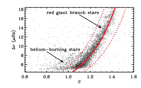
Our initial selection of stars was based on the analysis by Stello et al. (2013) of 13,412 red giants from which we adopt their measurements of $\Delta\nu$ and $\nu_{\mathrm{max}}$, as well as their estimates of stellar mass based on the combination of those seismic observables with photometrically-derived effective temperatures using scaling relations (see Stello et al. 2013,  for details). In order to select only red giant branch stars from this sample we follow the approach by Stello et al. (2016). We selected all 3,993 stars with $\nu_{\mathrm{max}}$ $>50\,$$\mu$Hz and $M<2.1\,$M_⊙, which based on stellar models is expected to select only red giant branch stars (e.g. Stello et al. 2013). However, this selection do not take measurement uncertainties in $\nu_{\mathrm{max}}$ and $M$ into account, possibly introducing some helium-core burning stars into our sample towards the lower end of the $\nu_{\mathrm{max}}$ bracket. We therefore performed a few additional steps to further reduce the possible ‘contamination’ by helium-burning stars in our sample.

First, we derived the offset from zero of the harmonic series of radial modes, known as $\varepsilon$ in the asymptotic relation, $\nu=\Delta\nu(n+\ell/2+\varepsilon)$, where $\nu$ is the mode frequency and $n$ is the radial order. This offset is known to be different for helium-burning stars (Kallinger et al. 2012; Christensen-Dalsgaard et al. 2014) relative to red giant branch stars of similar density, and hence has diagnostic power to distinguish the two types of stars. To measure $\varepsilon$ we calculated frequency power spectra for each star using long-cadence ($\Delta t\simeq 29.4\,$minutes) Kepler data obtained between 2009 May 2 and 2012 Oct 3, corresponding to observing quarters 0–14, or a total of about 54,000 data points per star. We used the method by Huber et al. (2009) to fit and remove the background noise profile of the spectra, and then selected the central $\pm 2$$\Delta\nu$ spectral range around $\nu_{\mathrm{max}}$, which we folded with an interval of $\Delta\nu$. The folded spectrum was smoothed by a Gaussian function with a full-width-half-maximum of 0.1$\Delta\nu$, and correlated with a model of the spectrum (Figure 1).

Figure 1: (a) Folded and smoothed spectrum (black curve) of the central 4$\Delta\nu$-wide region around $\nu_{\mathrm{max}}$ of a normal star (KIC2141255). Regions dominated by modes of degrees, $\ell=0$, 1, 2, and 3 are indicated. The red curve shows the model shifted to the position resulting in the largest correlation with the data. (b) Correlation versus shift between model and data. (c) and (d) The same as (a) and (b), but for a star with suppressed non-radial modes (KIC4348666).

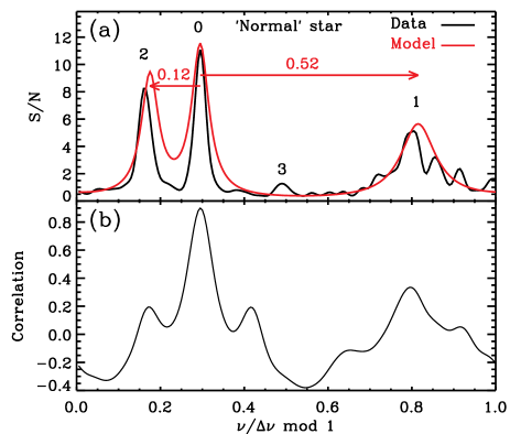
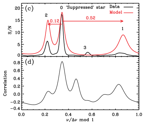
Each spherical degree in the model was described by a Lorentzian profile with relative heights of 1.0, 0.5, and 0.8 for the $\ell=0$, $\ell=1$, and $\ell=2$ modes, and widths of 5%, 10%, and 5% of $\Delta\nu$, respectively. The Lorentzian profiles were centered relative to each other with the one representing quadrupole modes being 0.12$\Delta\nu$ to the left of the radial mode profile, and the one representing the dipole modes being 0.52$\Delta\nu$ to the right of the radial mode following the results by Huber et al. (2010) (see Figure 1). The shift between data and model providing the largest correlation was adopted as $\varepsilon\!\!\mod 1$. Only the 3,721 stars with $\varepsilon$ within $\pm 0.1$ of the $\Delta\nu$-$\varepsilon$ relation by Corsaro et al. (2012) ($\varepsilon=0.634+0.63\log(\Delta\nu)$) were kept in our sample (see Figure 2).

Figure 2: $\Delta\nu$ versus $\varepsilon$ of the 3,993 red giants from the Stello et al. (2013) sample with $\nu_{\mathrm{max}}$ $>50\,$$\mu$Hz and $M<2.1\,$M_⊙. The solid red curve shows the relation by Corsaro et al. (2012), and the dotted red curves show the relation shifted by $\pm 0.1$.

Second, we cross matched our remaining sample with the stars identified as burning helium by Stello et al. (2013) and Mosser et al. (2014) based on their dipole-mode period spacings. We found 86 helium-burning stars this way, which we removed. We note that all but eight of these helium-burning contaminants had $\nu_{\mathrm{max}}$ $<70\,$$\mu$Hz (and all $<85\,$$\mu$Hz). Although our remaining sample could potentially still include some helium-burning stars if they were not in the Stello et al. (2013) and Mosser et al. (2014) samples, the above cross match indicates such contaminants would most likely have $\nu_{\mathrm{max}}$ $<70\,$$\mu$Hz. As a final check, we visually inspected the power spectra of the remaining sample (3,635 stars), which led to the removal of 24 stars that appeared to be helium-core burning or had spectra of such poor quality (low signal-to-noise or bad window function) that the stellar classification was ambiguous.

3.2 Mode visibility measurements

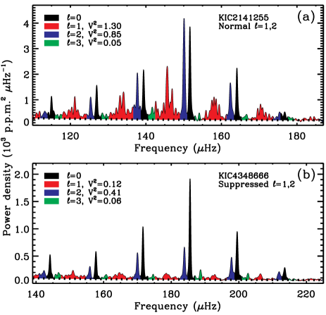
To measure the mode visibilities, we first needed to identify the regions in the power spectra dominated by the different modes. Here, we used the $\varepsilon$ values found in the previous step (Sect. 3.1) to locate the four central radial modes closest to $\nu_{\mathrm{max}}$, and followed the approach by Stello et al. (2016) for masking the parts of the spectra dominated by $\ell=0$, $\ell=1$, $\ell=2$, and $\ell=3$ modes. The regions we chose were $\varepsilon-0.06<(\nu/\Delta\nu\mod 1)<\varepsilon+0.10$ for $\ell=0$, $\varepsilon+0.25<(\nu/\Delta\nu\mod 1)<\varepsilon+0.78$ for $\ell=1$, $\varepsilon-0.22<(\nu/\Delta\nu\mod 1)<\varepsilon-0.06$ for $\ell=2$, and $\varepsilon+0.10<(\nu/\Delta\nu\mod 1)<\varepsilon+0.25$ for $\ell=3$. In this way, the entire 4$\Delta\nu$-wide central part of the spectrum was divided up into distinct segments associated with either $\ell=0$, $\ell=1$, $\ell=2$, or $\ell=3$ modes. In Figure 3 we show a couple of representative spectra with the results of the masking, identifying the different mode degrees. See also Figure 1 in Stello et al. (2016) who used the exact same scheme.

Figure 3: Representative power spectra of two red giants from our sample. For clarity the spectra have been smoothed by 0.03$\Delta\nu$, which partly merges the power from individual mixed modes into one broad peak around each acoustic resonance. The colored regions indicate the integrated power associated with each mode of degree $\ell=0$, 1, 2, and 3. The horizontal dashed curves shows the estimated noise profile (a) Star with normal mode visibility, $V^{2}$, of the non-radial modes. (b) Star with low mode visibilities in both dipole and quadrupole modes, but normal octupole mode visibility.

Finally, the mode visibilities, $V^{2}$, of the non-radial modes were derived as the ratio of the total mode power of the segments associated with a given degree relative to the total radial mode power. For this we used the background corrected spectra described in Sect. 3.1. We note that the uncertainty in the background estimation introduces measurement scatter on top of the intrinsic spread in the visibilities, potentially pushing intrinsically low values of $V^{2}$ below zero. Rejecting those stars or artificially pushing them up to $V^{2}=0$ would be statistically incorrect and bias our measurements of the average $V^{2}$.

4 Results

4.1 The dipole modes revisited

In Figure 4 we show our measurements of the dipole mode visibility as function of $\nu_{\mathrm{max}}$. We denote the stars below the dotted line as the dipole-suppressed sample, as opposed to the ‘normal’ stars. As shown in Fuller et al. (2015) and Stello et al. (2016), the predicted visibilities of the suppressed dipole modes (solid lines) match the observations remarkably well, and with normal stars on average being less massive. Here, we show that the prediction for the dipole-mode suppression is insensitive to stellar mass for the typical mass range of the Kepler red giants (the solid black curves fall almost on top of each other), which is also what we observe in the data. The slight dependence on mode lifetime, $\tau$, is illustrated by comparing the black curves (all $\tau=20\,$days) with the gray curves based on a $1.7\,$M_⊙ track just above ($\tau=10\,$days) and below ($\tau=40\,$days) the black curves. We find no variation in the average visibility ($V^{2}_{\ell=1}=1.35$) and its scatter for the normal stars as a function on $\nu_{\mathrm{max}}$.

Figure 4: Visibility of dipole modes ($V^{2}_{\ell=1}$) for 3,611 red giants below the red giant branch luminosity bump. Stars evolve from right to left, and their approximate $\log g$ values are shown on the top axis. The rms scatter in $V^{2}_{\ell=1}$ is 0.26 (or 20%) for the normal stars. The color of each symbol indicates the stellar mass according to the scale on the right-hand side. The solid black lines are the predicted visibilities from 1.1M_⊙, 1.3M_⊙, 1.5M_⊙, 1.7M_⊙, and 1.9M_⊙ models adopting an average mode lifetime of 20 days in agreement with Corsaro et al. (2015) (Sect, 2). The solid gray curves are the predicted visibilities from 1.7M_⊙ models for mode lifetimes of 10 days (highest $V^{2}_{\ell=1}$) and 40 days (lowest $V^{2}_{\ell=1}$). The dotted fiducial line, adopted from Stello et al. (2016), separates dipole-suppressed and normal stars. The observed dipole visibilities are identical to those by Stello et al. (2016).

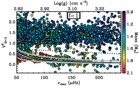
In an attempt to determine if the dipole-suppressed sample is somehow distinct other than by their mass (Stello et al. 2016), we do not find them to be statistically different in terms of their distance and position on sky. If we focus on the mass range $1.5<M$/M_⊙ $<1.8$, where we find the highest number and fraction (50–60%) of dipole-suppressed stars (Stello et al. 2016), the dipole-suppressed sample is on average slightly more metal poor (by $0.045\pm 0.017$ dex) than the normal stars, and slightly hotter (by $26.9\pm 8.9\,$K) (based on SDSS-APOGEE DR12, Alam et al. 2015).

4.2 The quadrupole and octupole modes

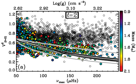
The quadrupole and octupole visibilities are shown in Figures 5 (a) and (b), respectively. Here, we only show the dipole-suppressed sample as filled symbols, to make it easier to distinguish them from the normal population shown as empty symbols. While less dramatic than the dipole modes, the quadrupole modes show significant reduction in mode power for the dipole-suppressed sample. The least evolved stars ($210<\,\,$$\nu_{\mathrm{max}}$/$\mu$Hz $<240$) show on average $V^{2}_{\ell=2}=0.350\pm 0.053$, compared to $V^{2}_{\ell=2}=0.688\pm 0.003$ for all the normal stars, corresponding to 49% reduction in power. Although there is overall good agreement between the predictions and the observations, the trend of the visibility as a function of $\nu_{\mathrm{max}}$ is predicted to be steeper than observed if we, as done here, assume a fixed mode lifetime along the red giant branch (Figure 5(a)). We used a lifetime of $20\,$days, which is representative for the average value found by Corsaro et al. (2015). This assumption could, at least partly, explain the discrepancy, because the observed mode lifetimes are most likely increasing as red giants evolve towards lower $\nu_{\mathrm{max}}$ and lower $T_{\mathrm{eff}}$. The variation in mode lifetime was found to be roughly 50% by Corsaro et al. (2015, their Figure 7) across a sample spanning a $\nu_{\mathrm{max}}$ range of $\sim 110-160\,$$\mu$Hz (their Table A.2). Our sample span a much larger $\nu_{\mathrm{max}}$ range, and for reference we therefore also show the $1.7\,$M_⊙ tracks in gray with factors of two difference in mode lifetime; 10 and 40 days, respectively. Based on this, we conclude that an increasing mode lifetime along the red giant branch could possibly explain the apparent discrepancy of the predicted versus observed trend seen in Figure 5(a). A mode lifetime of $\sim 15\,$days at $\nu_{\mathrm{max}}$ $=200\,$$\mu$Hz and a lifetime of $\sim 30\,$days at $\nu_{\mathrm{max}}$ $=70\,$$\mu$Hz would provide a better match to the data. However, we note that the predicted visibilities of the suppressed sample depends somewhat on the overshoot beyond classical Schwarzschild implemented in the stellar models (Cantiello et al. 2016, in prep.), so we defer a more thorough analysis to future work, but point out here the possibility of constraining either the mode lifetime or the overshoot given independent measurements of the other.

Figure 5: (a) Visibility of quadrupole modes for the same stars as shown in Figure 4. The notation follows that of Figure 4 except only the dipole-suppressed stars (those below the dotted line in Figure 4) are shown by filled symbols. The observed rms scatter in $V^{2}_{\ell=2}$ is 0.14 (or 20%) for the normal stars. (b) The same as panel (a) but for octupole modes. Here, the observed $V^{2}_{\ell=3}$ scatter is 0.05 (84%).

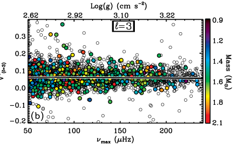
Turning to the octupole modes (Figure 5(b)), we see no significant effect of the suppression, as anticipated by theory (solid black curves) because they are almost purely acoustic envelope modes. We find the average visibilities to be $V^{2}_{\ell=3}=0.0591\pm 0.0009$ for the normal stars, and $V^{2}_{\ell=3}=0.0577\pm 0.0018$ for the dipole-suppressed sample, which are the same within $1\sigma$. In Figure 5(b) we do not show the tracks of different mode lifetimes because they are essentially indistinguishable from the black curves.

4.3 Discussion

Both the evolution of the predicted mode visibility as a function of $\nu_{\mathrm{max}}$ (for fixed spherical degree) and its dependence on mode degree (for fixed $\nu_{\mathrm{max}}$) are essentially determined by the difference in coupling between the core and envelope as the star evolves (or as seen by modes of different degree). The key aspect of this predicted behavior is that there is perfect trapping of the mode energy leaking into the core by the suppression mechanism. Hence, given the agreement reported here between theory and observations for both $\ell=2$ and $\ell=3$ modes, in addition to what is seen for dipole modes, supports this notion that the mode suppression mechanism indeed traps almost, if not, all the energy that leaks into the core region.

The theoretical predictions presented in Figures 4 and  5 are derived relative to non-suppressed stars, and are hence scaled to the observed average visibilities of the normal stars. We note that the absolute scale of the observed visibilities reported here are not directly comparable with expectations for the normal stars (Ballot et al. 2011) because we simply integrated the power over fixed regions of the spectrum in terms of $\Delta\nu$. Due to the presence of mixed modes, which strictly speaking exist across the entire spectrum, small amounts of power (from gravity-dominated modes far from the acoustic resonant frequencies) from one degree of modes will be present in the regions that we associate with modes of another degree. Direct comparisons would therefore need to be based on simultaneous fitting of model profiles to all the modes in the spectrum, which is currently not practically possible for large numbers of stars (Corsaro et al. 2015). Similarly, any differences between the average visibilities reported here and those by Mosser et al. (2012), are most likely due to slight different choices for the mode integration regions in the two studies.

5 Summary and outlook

We have measured oscillation mode power in over 3,600 red giant stars, and compared our results to theoretical predictions based on the “magnetic greenhouse” mechanism proposed by Fuller et al. (2015) for dipole mode suppression. Our results from modes of spherical degrees $\ell\leq 3$, provide strong support for one of the main assertions of the theory behind the mode suppression – all mode energy leaking into the g-mode cavity of a star is efficiently trapped or dissipated. Specifically, we confirm the up to almost 100% suppression for dipole modes previously shown and measure for the first time up to 49% suppression on average of the quadrupole modes and no suppression of the octupole modes. We find it likely that a variation in the mode lifetime along the red giant branch could explain the small difference in slope between our prediction and the observations in the $V^{2}_{\ell=2}$ versus $\nu_{\mathrm{max}}$ diagram. However, the variation required needs to be confirmed by measurements of the mode lifetime of radial modes for a robust sample of stars with $\nu_{\mathrm{max}}$ around 220$\mu$Hz and 70$\mu$Hz.

Further tests of the magnetic greenhouse effect could be implemented with determinations of the lifetimes of the suppressed dipole modes, or the measurement of suppressed dipole mode visibilities in helium-burning clump stars (Cantiello et al. 2016 in prep.)