The slowest spinning X-ray pulsar in an extragalactic globular cluster

Abstract

Neutron stars are thought to be born rapidly rotating and then exhibit a phase of a rotation-powered pulsations as they slow down to 1–10 s periods. The significant population of millisecond pulsars observed in our Galaxy is explained by the recycling concept: during an epoch of accretion from a donor star in a binary system, the neutron star is spun up to millisecond periods. However, only a few pulsars are observed during this recycling process, with relatively high rotational frequencies. Here we report the detection of an X-ray pulsar with $P_{\rm spin}=1.20$ s in the globular cluster B091D in the Andromeda galaxy, the slowest pulsar ever found in a globular cluster. This bright (up-to 30% of the Eddington luminosity) spinning-up pulsar, persistent over the 12 years of observations, must have started accreting less than 1 Myr ago and has not yet had time to accelerate to hundreds of Hz. The neutron star in this unique wide binary with an orbital period $P_{\rm orb}=30.5$ h in a 12 Gyr old, metal rich star cluster, accretes from a low mass, slightly evolved post-main sequence companion. We argue that we are witnessing a binary formed at relatively recent epoch by getting a $\sim$0.8$M_{\hbox{$\odot$}}$ star in a dynamical interaction – a viable scenario in a massive dense globular cluster like B091D with high global and specific stellar encounter rates. This intensively accreting non-recycled X-ray pulsar provides therefore a long-sought missing piece in the standard pulsar recycling picture.

1. Introduction

Around 2000 pulsars are known, where the majority of these are ’regular’ pulsars which have pulse periods between tens of milliseconds to approximately a second, and magnetic field strengths of $\sim$10¹² G (Manchester et al., 2005). These pulsars show a general spin down to longer periods. However, a few hundred of these pulsars show much shorter periods, of the order a millisecond, along with lower magnetic fields of $\sim$10⁸ G. It is believed that these millisecond pulsars (MSPs) are the descendants of neutron stars/pulsars found in X-ray binaries. Accretion onto a neutron star from a close companion is believed to transfer angular momentum to the neutron star, spinning it up to periods of milliseconds (Alpar et al., 1982; Radhakrishnan & Srinivasan, 1982). This is strongly supported by both the discovery of a MSP in an X-ray binary system (SAX 1808.4-3658, Wijnands & van der Klis, 1998) and the presence of kilo-Hertz Quasi-Periodic Oscillations in many LMXBs, which have been found to show millisecond pulsation periods (see van der Klis, 1998, and references therein). More recently, Archibald et al. (2009) showed that the previously accreting millisecond pulsar FIRST J102347.67+003841.2 had ceased to accrete and radio pulsations could subsequently be observed, thus supporting the ’recycled’ pulsar idea (see Patruno & Watts (2012) for a review).

Many of the known MSPs are found in Galactic globular clusters (GCs), where as of the end of 2015, almost 140 MSPs have been detected. Globular clusters are dense spherical systems of $\sim$10⁴–10⁶ old stars (e.g. Hénon, 1961). Their old age implies that they should also contain many compact objects (e.g. Hut et al., 1992). Stellar encounters, which are extremely rare in lower density regions, can occur in globular clusters on time-scales comparable with or less than the age of the Universe. This would indicate that many Galactic globular cluster stars have undergone at least one encounter in its lifetime. Encounters between stars is one way in which binaries can be produced. The encounter rate ($\Gamma$) due to tidal capture (Fabian et al., 1975) is proportional to the encounter cross-section, the relative velocity of the stars and the number density of stars in the cluster (core). Both primordial binary systems and those formed due to encounters should exist in globular clusters due to the dense environments, but encounters between a binary and either a single star or a binary system would more readily occur as the cross sections are significantly larger, thus increasing the likelihood of an encounter. This explains the large number of recycled pulsars that we observe in GCs.

However, a small number (6) have periods greater than 0.1 s and these pulsars have not yet been fully recycled. The longest of these, B 1718-19 in NGC 6342, has a period of 1.004 s and a magnetic field of $\sim 10^{12}$ G, typical of a ’regular’ pulsar. It appears to be a young pulsar, with a characteristic age of 1 $\times$ 10⁷ years (Lyne et al., 1993). Lyne et al. (1993) propose that this young pulsar originated either from a collision between an old neutron star and a cluster star, or that a white dwarf accreting from a companion underwent an accretion induced collapse (Michel, 1987). Verbunt & Freire (2014) suggest that the current main-sequence companion of an old neutron star in that system has replaced the original one in an exchange encounter.

Following the recent detection of coherent pulsations from an ultra-luminous X-ray source (ULX) in the M82 galaxy ($\simeq$3.5 Mpc away) using NuSTAR data (Bachetti et al., 2014), which showed that this bright source was in fact a neutron star, we started to search archive XMM-Newton data to find similar sources, in order to address questions such as how can such super-Eddington luminosities be possible in a neutron star (see e.g. Mushtukov et al., 2015; King & Lasota, 2016, for further discussion).

In this paper we describe the analysis that made it possible to detect a 1.2 s pulsar in the X-ray binary 3XMM J004301.4+413017, associated with the globular cluster B091D from the Revised Bologna Catalog of M31 (catalog ) globular clusters (RBC V.5; Galleti et al., 2004), using public data. For brevity we denote the pulsar XB091D after its host globular cluster designation. This is the first persistently accreting X-ray pulsar hosting a neutron star detected in M31 (catalog ), and it also has the longest period among all known pulsars (rotation-powered and accreting) in globular clusters, being more than an order of magnitude slower than the mildly recycled accreting pulsar from Terzan 5 globular cluster (Papitto et al., 2011). We note that this pulsar has also recently been detected by Esposito et al. (2016), but these authors interpret the nature of this source quite differently. In this paper, we discuss possible evolutionary scenarios that may produce such slowly rotating neutron stars in globular clusters.

The content is organized as follows: Section 2 briefly describes the XMM-Newton photon database (which will be described in detail elsewhere) and the dataset used for the initial pulsation detection, as well as the XMM-Newton pulsar factory analysis methods which resulted in the automated detection of the pulsed X-ray emission; Section 3 covers the manual blind search for pulsed emission in all available XMM-Newton data for this source and the determination of source’s orbital parameters; Section 4 and 5 summarize our findings on the timing and spectral properties of this source which are then discussed in Section 6 where we also argue on the possible origin and evolution of this system.

2. Pulsations search data and methods

2.1. Photon database

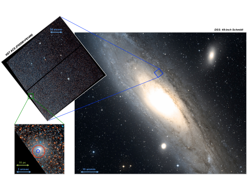
Figure 1.— The position of the XB091D and its host globular cluster B091D in the Andromeda galaxy in several scales – using colored images from the Digitized Sky Survey and HST ACS. On the zoomed inset in the bottom left corner, we overplot the 95% confidence level X-ray positional uncertainties from the Chandra (red circle) and XMM-Newton (blue circle) catalogs.

For this study we created a database of all photons registered by the EPIC/pn detector of the XMM-Newton satellite and operated in imaging mode during the 7781 observations that took place between 2000 and mid 2013. These are the same observations that were used to compile the 3XMM-DR5 catalog (Rosen et al., 2015). The photon data were taken from the event lists called PIEVLI files publicly available from the XMM-Newton science archive. These are science-ready data products that come from the pipeline run by the XMM-Newton Survey Science Centre (XMM SSC). Each file is a binary table with one row per event that contains the following information: (a) event time (satellite clock), (b) raw CCD pixel and projected sky coordinates relative to the nominal pointing position, (c) corrected and uncorrected event energy; (d) event quality flag; (e) CCD number. Each PIEVLI file also contains good time intervals determined separately for each pn CCD by the XMM SSC pipeline software. We point out that it is not necessary to retrieve the complete XMM-Newton observation archive (ODF archive) for the massive scale timing analysis with the XMM-Newton.

These event lists represent the lowest and most detailed data level we use for initial timing studies. These are accompanied by higher level data in the form of the 3XMM-DR5 catalog of X-ray sources and their individual observations acting essentially as an index for the navigation within the photon database. The connection between these two very different sets of information is achieved by means of the known transformation between pixel coordinates of the events and world coordinates of the X-ray sources from the 3XMM-DR5 catalog. We used the World Coordinate System (WCS) transformation data available for every EPIC/pn exposure in the PIEVLI file. In this fashion one can make event extraction for any detection from the 3XMM-DR5 catalog using its world coordinates, right ascension and declination.

The catalog of X-ray sources was cross-matched with other catalogs of astrophysical objects in order to find possible counterparts and determine the source type or location within a galaxy. This gives us the possibility to easily extract arbitrary photon lists of e.g. all photons coming from the M31 (catalog ) galaxy, or all photons from known magnetars.

The last stage before being able to launch our timing analysis codes over the sequence of extracted photon lists is the barycentric correction, i.e. correcting the event times to the Solar System barycenter. For this purpose we used the XMM-Newton orbit files fed to the barycen task from the XMM-Newton SAS version 13.5 software and the source positions from the 3XMM-DR5 catalog.

We note that it is now possible to access this photon database as well as the 3XMM-DR5 catalog data through the convenient web interface that we developed while working on the 3XMM-DR5 catalog compilation and this project. In particular, one can extract barycentered photons in arbitrary regions from the observation level event lists using nothing but a web browser. More details on this website for the quick-look science analysis of the XMM-Newton data will be presented in a separate paper (Zolotukhin et al., in prep.)

2.2. Pulsar factory analysis software

The photon database provides a way to easily extract calibrated and barycentered event lists for arbitrary sets of astrophysical sources observed with the EPIC/pn camera on board the XMM-Newton satellite. We developed an analysis software aimed at finding coherent pulsations in the photon database, optimized for high throughput.

It consists of few analysis layers. First, for each event list it produces the power density spectrum (PDS) adapting the time binning so that the Nyquist frequency is well above 2 kHz and the total number of bins between gaps in the light curve is factorable with small prime numbers for better performance with the numpy FFT algorithm. In the PDS the algorithm searches for peaks exceeding the 99 per cent detection level, including the number of trials, following the standard rules from Leahy et al. (1983). If such peaks are found, it launches the $Z^{2}_{n}$ test (Buccheri et al., 1983) in the vicinity of their frequencies. If a peak from the PDS is confirmed with the $Z^{2}_{n}$ test, an accelerated search with the PRESTO code (Ransom, 2001) is launched to constrain further or discard this pulsation frequency candidate. As the final step of the automated procedure the pulsar factory checks this frequency in other observations of this source from the 3XMM-DR5 catalog. If the detection is highly significant ($>$$n\sigma$, where $n$ can vary between runs) or the same frequency is found in other detections, an operator is notified.

We first tested the XMM-Newton pulsar factory code using XMM-Newton data on a set of known X-ray bright magnetars from the McGill Online Magnetar Catalog (Olausen & Kaspi, 2014). After achieving the stable detection of known coherent pulsation periods in this automated regime, we launched a larger period search on the unstudied sample of X-ray sources in the catalog. The M31 (catalog ) galaxy was an obvious choice of survey region for its large number of known X-ray sources and its relatively low distance, and was included in our first survey.

Table 1Best orbital solution found in this paper.

Parameter	Value
$P_{\rm orb}$	1.27101304(16) d
$T_{\rm asc}$	MJD 56104.791(26)
$a\sin i/c$	2.89(13) l-sec
$e$	$<$0.003

Note. — Brackets indicate 1-$\sigma$ uncertainties, as returned by TEMPO2. The upper limit on the eccentricity is the maximum uncertainty returned by the ELL1 model, for values of the eccentricity always consistent with 0.

Table 2XMM-Newton observations used for timing analysis in this study and its main results.

ObsID	Obs. start	Exposure	$P_{\rm spin}$	$S$ / d.o.f.	Pulse depth
	UTC	(s)	(s)
0112570101	2002-01-06 18:45:45	64317	1.203898(49)	8.7	$0.33\pm 0.07$
0405320701	2006-12-31 14:24:50	15918	1.203731(11)	4.1	$0.28\pm 0.08$
0405320901	2007-02-05 03:44:24	16914
0505720201	2007-12-29 13:42:13	27541	1.203738(10)	7.3	$0.20\pm 0.05$
0505720301	2008-01-08 07:01:05	27219
0505720401	2008-01-18 15:11:47	22817
0505720501	2008-01-27 22:28:21	21818
0551690201	2008-12-30 03:27:52	21916	1.203662(8)	5.0	$0.23\pm 0.05$
0551690301	2009-01-09 06:19:54	21918
0551690501	2009-01-27 07:23:03	21912
0551690601	2009-02-04 13:21:03	26917
0600660201	2009-12-28 12:42:54	18820	1.203675(13)	4.2	$0.25\pm 0.08$
0600660501	2010-01-25 02:39:14	19715
0650560301	2011-01-04 18:10:16	33415	1.203651(8)	9.1	$0.31\pm 0.06$
0650560401	2011-01-15 00:16:57	24316
0650560601	2011-02-03 23:58:12	23918
0674210201	2011-12-28 01:07:36	19034	1.203634(13)	4.9	$0.35\pm 0.09$
0674210301	2012-01-07 02:47:01	15433
0674210401	2012-01-15 15:00:38	19916
0674210501	2012-01-21 12:22:03	17317
0690600401	2012-06-26 06:29:43	122355	1.203698(4)	20.6	$0.23\pm 0.03$
0700380501	2012-07-28 15:16:27	11914
0700380601	2012-08-08 23:08:08	23916
0701981201	2013-02-08 22:19:55	23918	1.20373(13)	7.0	$0.45\pm 0.14$

Note. — Available observations were split into 9 blocks which were analysed with the assumption that NS spin period $P_{\rm spin}$ does not change much within them. $S$ / d.o.f. is the statistical significance of the obtained solution as defined in the Appendix A.1. Pulse depth (also referred as pulsed fraction) is defined as quantity $A$ there as well. Uncertainties represent $1\sigma$ confidence interval.

3. Detection and orbital parameters

During the M31 (catalog ) test run, the automated XMM-Newton pulsar factory algorithm detected pulsations, at about the same period, in 3 observations (ObsIDs: 0112570101, 0505720301, P0650560301) of the source 3XMM J004301.4+413017. The $Z^{2}_{n}$ test triggered by the detection confirmed the candidate. These detections are fully reproducible online from the source’s event extraction pages, e.g. for observation 0112570101: http://xmm-catalog.irap.omp.eu/pievli/101125701010068.

In order to look for the detected pulsation in more ObsIDs, we ran an accelerated search with PRESTO in all ObsIDs containing the source. The very high values of period derivative required by the accelerated search, the clear improvement of detection significance when adding a second derivative in the search, and the shape of the track in the phaseogram shown by PRESTO, pointed towards the presence of orbital modulation. Largely following the same procedure described in Bachetti et al. (2014), we cut the two longest ObsIDs into chunks, 10–30 ks long, and ran an accelerated search with custom-made software, searching the solution in the $\nu-\dot{\nu}$ plane (where $\nu$ indicates the pulse frequency) that yielded the highest $Z^{2}_{2}$ statistics.

Inside the long ObsIDs (0112570101, 0690600401) the best-solution frequency and frequency derivative clearly followed a sinusoidal law with a period between 1 and 2 days, as expected from orbital modulation. We fitted simultaneously the two values of frequency and frequency derivative in ObsID 0690600401 with the expected variation due to orbital motion, and obtained a first estimate of the orbital parameters ($P_{\rm orb}\sim 1.2$ d, $a\sin i/c\sim 2.60$ l-sec, $T_{\rm asc}\approx{\rm MJD}56104.789$, where $a\sin i/c$ is the projected semi-major axis and $T_{\rm asc}$ the time of passage through the ascending node). Starting from the first rough estimate of these parameters and, by trial-and-error, trying to align the pulses in the phaseogram in the chunks first, then calculating TOAs with a custom implementation of the fftfit method (Taylor, 1992) and using TEMPO2 to fit an orbital solution with the ELL1 model, we reached a solution valid to ObsID 0690600401. We then applied the solution to the other long ObsID, refining the orbital parameters so that every residual orbital modulation was eliminated by assuming a constant spin through the observation. The solution found in this way is the following: $P_{\rm orb}\approx 1.2695$ d, $a\sin i/c\approx 2.886$, $T_{\rm asc}\approx 56104.7907$. Then, we addressed the ObsIDs in between, using “quantized” values of the orbital period that conserved the ascending node passages close to the two long ObsIDs. For every value, we calculated the scatter that it produced on the TOAs and selected the one that produced the lowest scatter. The eccentricity fitted by ELL1 was always consistent with 0 at the $\sim 2\sigma$ level, with an uncertainty of 0.002–0.003. We use this last number as an upper limit on the eccentricity. The full solution is in Table 1.

We used this solution to look for pulsations in the remaining ObsIDs and refine the estimate. In the next section we describe this procedure.

4. Refined timing analysis

Except a few cases (ObsIDs: 0112570101, 0650560301, 0690600401), all other individual observations yield poor photon statistics in order to determine the pulsation period and the pulse shape with enough statistical significance for detailed interpretation.

Therefore, we attempted the search of coherent pulsations by combining several datasets spanning 2 to 5 months in different years of observations by assuming that the period did not change among individual observations within each block. First, we corrected all the photon arrival times using the orbital elements of the binary system reported above. Then we used the period grid search using the $S$ statistics with regularization (see Appendix for details) leaving the orbital phase as an additional free parameter.

Then, for each year we started with the first observation typically taken in late December or early January and then started adding observations checking that the $S$ statistics around the probable period, according to the increase in the exposure time suggesting that the pulsations are still coherent. If the $S$ statistics (Leahy et al., 1983) did not increase or decrease when we added the additional observation, we concluded that the period changed significantly and started a new block. The results of our timing analysis are provided in Table 2 and the blocks of observations used for coherent searches are separated with horizontal lines. We estimated uncertainties of the period measurements analytically from the photon statistics, exposure time, and the pulse properties as explained in the Appendix. In Fig. 2 we provide the 9 recovered pulse profiles between 2002 and 2012.

We note that when correcting photon arrival times using the orbital solution of Esposito et al. (2016), we were only able to get sufficient pulsations significance in three observations (0112570101, 0650560301, 0690600401), whereas in all remaining datasets the pulsating signal was not detected because it was smeared. At the same time the orbital solution obtained in this study allows to significantly detect pulsations in all observations listed in Table 2. Though these two orbital parameter estimates agree on the order of magnitude with each other, the solution presented here is more precise.

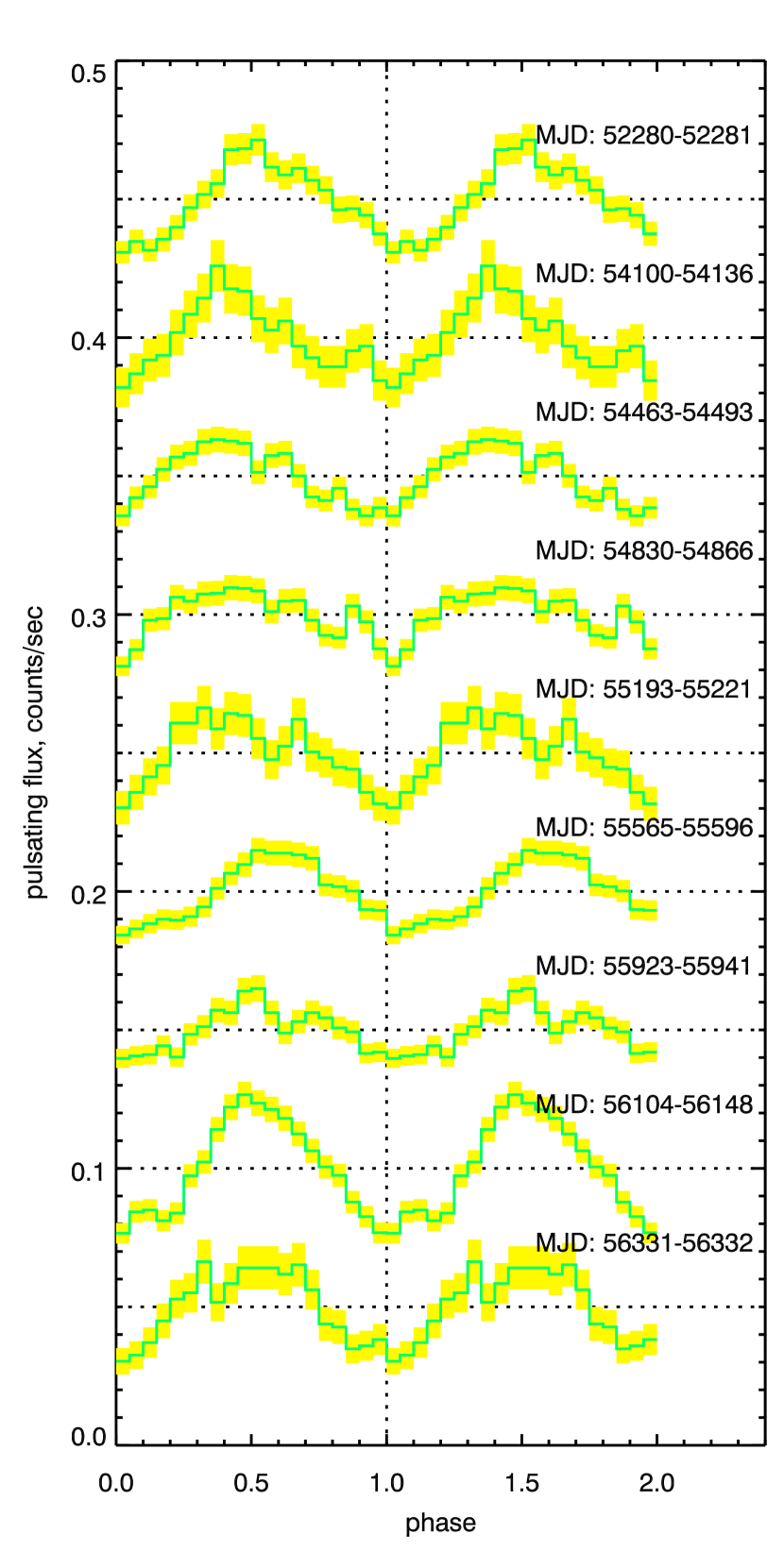
Figure 2.— Recovered pulse profiles of XB091D obtained from the search for coherent pulsations using the regularized $S$ statistics in 9 combined datasets listed in Table 2. The shift along the Y axis is arbitrary and is made for clarity.

This analysis of combined datasets reveals a spin-up trend observed in XB091D which is otherwise hard to be detected in individual observations, see Fig. 3. Despite at least one probable $\dot{P}$ sign change (note e.g. a period increase in the next to last dataset comprising observations from Jun to Aug 2012), it is likely that the neutron star spins up. On average the spin-up rate amounts to $\dot{P}\approx-5.7\times 10^{-13}$ s s^-1 if we consider all 9 period estimates obtained, or $\dot{P}\approx-7.1\times 10^{-13}$ s s^-1 if we reject the most recent dataset, having the largest period uncertainty.

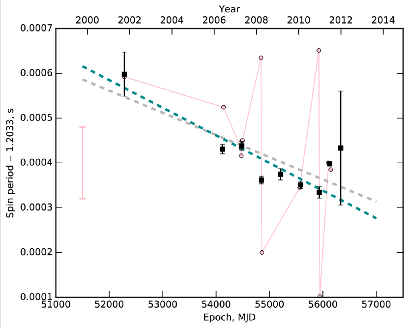
Figure 3.— Evolution of neutron star spin period. Spin period estimates obtained from individual observations are displayed in light color. They fluctuate strongly, however a typical uncertainty of individual measurement (plotted separately on the left) is large due to the poor photon statistics. What might be interpreted as a frequent change of $\dot{P}$ is, in reality, driven by these uncertainties. For this reason, we use the combined datasets listed in Table 2 to estimate better local period solutions. These are indicated by black dots in the plot. Their uncertainties are computed as per Appendix A.1 and illustrate the better quality of the combined datasets analysis. Note that in some cases the spin period estimates are not available from individual observations, however combining these datasets with adjacent ones often improves the pulse statistics. The dashed gray line is a linear fit to the period estimates from combined datasets. Dashed cyan line is the same but discarding the last period estimate due to its large uncertainty.

5. Spectral Analysis

We considered all imaging observations in which XB091D was in the f.o.v. of the EPIC instruments. Data reduction was performed with the standard epproc and emproc pipelines coming with the XMM-Newton Science Analysis Software (SAS v.14) and using the latest calibration files. From the raw event lists we selected high energy photons ($>$10 keV for the pn and between 10 and 12 keV for the MOS) and built light curves with 50 s binning, in order to identify and filter out time intervals affected by high particle background. Threshold count rates were set at 0.4 $\rm ct\,s^{-1}$ and 0.35 $\rm ct\,s^{-1}$ for the pn and MOS, respectively. We then used the interactive xmmselect task from the SAS to extract source and background spectra from the filtered event lists, starting with ObsID 0690600401 which has the largest counts statistics.

In this observation the source lies in the f.o.v. of all three EPIC cameras. We extracted source counts from a circular region of 25^′′ radius, while for the background we selected events from a nearby region free of sources within the same CCD. We applied the (FLAG==0)&&(PATTERN==0) filtering options during selection of pn events, in order to have the spectrum of the highest possible quality. For MOS counts we used the standard filtering flags, (#XMMEA_EM)&&(PATTERN<=12). The extracted spectra were then re-binned in order to have at least 40 and 25 counts per energy bin for the pn and MOS, respectively.

Spectral fitting was performed with XSPEC v12.9 (Arnaud, 1996). The spectrum of XB091D can be described by an absorbed power law with exponential cut-off, wabs(cflux*cutoffpl) in XSPEC. The spectrum is hard, with a photon index $\Gamma=0.20\pm 0.5$, a cut-off energy $E_{\rm cut}=4.6\pm 0.4$ keV, and low absorption, $n_{H}=3.79\times 10^{20}$ cm^-2, obtained from PN spectrum alone. We kept this value fixed in the simultaneous pn+MOS fit. This best-fit column density is in broad agreement with the expected value from the Dickey & Lockman (1990) in the direction of M31 (catalog ). The reduced chi square of the fit is 1.16 for 310 degrees of freedom. We present a plot of the best-fit folded spectrum and model for ObsID 0690600401 in Fig. 4.

We then analyzed all other observations, discarding those data sets where the source extraction region overlapped with CCD gaps or columns of bad pixels, and applying less stringent filtering options, (FLAG==0)&&(PATTERN<=4). In any case, given the lower count statistics, for all but ObsID 0700380601 a simpler absorbed power law model, wabs(cflux*powerlaw), is sufficient to fit the spectra adequately. We used the multiplicative component cflux, which returns the source’s flux directly as a parameter of the fit, to characterize variations with the epoch of the unabsorbed $0.3-10$ keV band luminosity, and of the hardness ratio HR, where $\rm HR=Flux_{5-10\,keV}/Flux_{0.3-5\,keV}$, assuming a distance to M31 (catalog ) of 752 kpc (Riess et al., 2012) and isotropic emission (Fig. 5). Intriguingly, the shape of the spectrum seems to be related with the luminosity of the source, where the harder spectra occur at higher luminosities, see Fig. 6.

Trudolyubov & Priedhorsky (2004) model the source X-ray spectrum with a hard power-law. Shaw Greening et al. (2009) similarly find its photon index to be $0.9\pm 0.1$ and interpret it as the high-mass X-ray binary (HMXB) nature of the source. Esposito et al. (2016) note that for some observations the absorbed power-law model does not provide satisfactory results and fit a blackbody + power-law model, as well as a cut-off power-law, which agree with our results within the uncertainties. They also note a similar ’harder-brighter’ correlation between the source luminosity and its spectral shape.

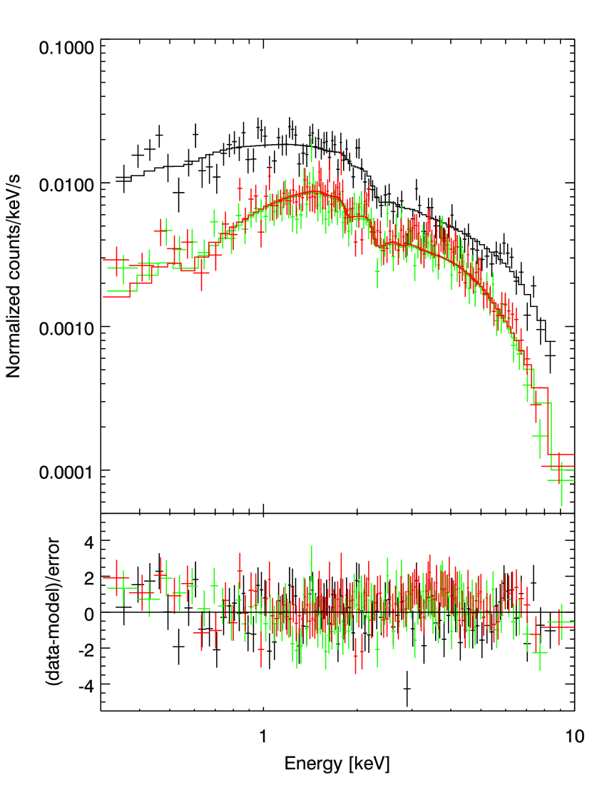
Figure 4.— Best-fit X-ray spectrum and folded model of XB091D during ObsID 0690600401. pn data are black, MOS1 are green and MOS2 are red. See main text for details.

Figure 5.— ${\it(Top)}$ Unabsorbed $0.3\textup{--}10$ keV luminosity of XB091D, in units of $10^{38}\,\rm erg/s$, versus the epoch of the observation. ${\it(Bottom)}$ Ratio of the unabsorbed fluxes estimated in the $5-10$ keV and $0.3-5$ keV bands, respectively. Error bars correspond to $1\sigma$ confidence limits.

Figure 6.— Hardness ratio versus the unabsorbed $0.3\textup{--}10$ keV luminosity of XB091D. Error bars correspond to $1\sigma$ confidence limits.

6. Discussion

We first estimate the chance association probability of this X-ray source with the globular cluster B091D projection without being physically associated, as Esposito et al. (2016) favor an interpretation with the pulsar not associated with the GC. The association was first suggested by Supper et al. (2001) based on ROSAT data and confirmed by Trudolyubov & Priedhorsky (2004) when the first XMM-Newton and Chandra data became available. These works, however, do not provide an assessment of the probability of the false association.

XB091D is included in 3XMM-DR5 with R.A.=00:43:01.478, Dec=+41:30:16.94 (J2000) and 1$\sigma$ positional uncertainty of 0.13^′′. These coordinates are computed as a weighted average of all individual detections, most of them being largely off-axis. The coordinates from ObsID 0690600401, the one with the smallest off-axis angle (1.82^′), are: R.A.=00:43:01.440, Dec=+41:30:17.30 (J2000), or 0.56^′′ away from the averaged coordinates, with a 1$\sigma$ positional uncertainty of 0.19^′′. Chandra Source Catalog Release 1.1 (Evans et al., 2010) includes this source as CXO J004301.4+413016 with coordinates R.A.=00:43:01.469, Dec=+41:30:16.80 (J2000) and the major semi-axis of the 95% confidence level error ellipse of 1.19^′′. The Bologna catalog gives B091D center coordinates as R.A.=00:43:01.446, Dec=+41:30:17.15 (J2000), which is consistent with the cluster center we find from the HST image within 0.15^′′ of its astrometric calibration uncertainty. Distances between the cluster center and the X-ray source coordinates are 0.41^′′ for the averaged XMM-Newton position, 0.17^′′ for ObsID 0690600401 position, and 0.44^′′ for the Chandra position. In our association probability calculations, we therefore assume that the X-ray source is located within 1^′′ from the cluster center.

There are 38 GCs (including candidates) between 14 and 16^′ projected distance from M31 (catalog )’s center in the Bologna catalog which yields their density $6.0\times 10^{-5}$ GCs per square arcsec at this angular distance from galaxy center. This gives a low probability ($1.2\times 10^{-2}$) of having a GC within 1^′′ of one of the 70 brightest X-ray sources from the 3XMM-DR5 catalog in M31 (catalog ). In fact, only 4 of the 70 brightest X-ray sources lie in this annulus. Therefore, their density of $6.3\times 10^{-6}$ per square arcsec is translated to the probability of only $7.5\times 10^{-4}$ of having a bright X-ray source within 1^′′ of any of the globular clusters. It is therefore highly likely that this X-ray source belongs to B091D globular cluster. Given the probability of coincidence, we assume below that the source belongs to the GC, and do not discuss alternative interpretations.

The detection of pulsations at $\sim 0.83$ Hz secures the identification of the source with a spinning neutron star. This is the first object of this class identified in the Andromeda Galaxy, and one of the most distant pulsars observed to date. Also given that XB091D resides inside the globular cluster it spins slower than any known sources in a GC (see Introduction) and about ten times slower than the slowest accreting pulsar in a globular cluster known previously, the $\sim 11$ Hz IGR J17480-2466 in Terzan 5 (Papitto et al., 2011). Its orbital period of 30.5 hr is also the longest known for accreting globular cluster binaries (see table 5 in Bahramian et al., 2014).

Given the maximum observed X-ray luminosity of the system $L_{\rm X}=1.2\times 10^{38}$ ${\rm erg\,s}^{-1}$ (see Fig. 5) which is close to Eddington, one can determine the corresponding mass accretion rate assuming that bolometric luminosity does not greatly exceed the X-ray luminosity: $\dot{M}=\frac{L_{\rm X}R_{\rm NS}}{GM_{\rm NS}}=1.0\times 10^{-8}$ $M_{\hbox{$\odot$}}$ yr^-1. We note that the observed X-ray variability of a factor $\simeq 3-4$ (see Fig. 5) excludes significant contribution from other unresolved X-ray sources residing in the same host globular cluster. We cannot completely rule out the possibility that we observe 2 superimposed X-ray sources residing in the same globular cluster, though the probability of this coincidence is relatively low: in our Galaxy there is only one globular cluster known to host two bright persistent LMXBs, M15 (White & Angelini, 2001). In case of the superposition we can only refer to the pulsed part of the flux (typically 20 per cent, see Table 2) as originating from this X-ray source. This would adjust our calculation of the accretion rate and the magnetic field below by a small factor, without affecting the important conclusions.

For a neutron star spinning with a 1.2 s period, the corotation radius is $R_{\rm C}=(GMP^{2}/4\pi^{2})^{1/3}\simeq 1890M_{1.4}^{1/3}$ km, where $M_{1.4}$ is the NS mass in units of $1.4$$M_{\hbox{$\odot$}}$.

We employ same approach as in Papitto et al. (2011) to estimate the lower and upper limits for the magnetic field of the neutron star given that it persistently accretes matter from the companion. It is reasonable to assume in this case that the accretion disk is truncated at the radius $R_{in}$ between the radius of the neutron star $R_{\rm NS}$ and the corotation radius $R_{\rm C}$: $R_{\rm NS}<R_{in}\mathrel{\hbox{\hbox to0.0pt{\hbox{\lower 4.0pt\hbox{$\sim$}}\hss}\hbox{$<$}}}R_{\rm C}=1890M_{1.4}^{1/3}$. The inner disk radius can be approximately defined (e.g. Ghosh & Lamb, 1978) from the balance between kinetic energy of the falling gas and the magnetic energy of the NS magnetosphere: $R_{in}\simeq 160M^{1/7}_{1.4}R_{6}^{-2/7}L_{37}^{-2/7}\mu_{28}^{4/7}$, where $R_{6}$ is the neutron star radius in units of 10 km, $L_{37}$ is the accretion luminosity in units of $10^{37}$ erg s^-1 and $\mu_{28}$ is the magnetic dipole moment of the NS in units of $10^{28}$ G cm³. After trivial transformations we obtain: $0.008L^{1/2}_{37_{\rm max}}<\mu_{28}\mathrel{\hbox{\hbox to0.0pt{\hbox{\lower 4.0pt\hbox{$\sim$}}\hss}\hbox{$<$}}}75L^{1/2}_{37_{\rm min}}$ We substitute the minimum ($L_{37_{\rm min}}=3.5$) and maximum ($L_{37_{\rm max}}=12.0$) observed X-ray luminosity into the resulting expression and obtain: $2.7\times 10^{8}\,{\rm G}<B\mathrel{\hbox{\hbox to0.0pt{\hbox{\lower 4.0pt\hbox{$\sim$}}\hss}\hbox{$<$}}}1.4\times 10^{12}\,{\rm G}$. This upper limit corresponds to the case of equilibrium rotation of the neutron star when the accretion disk is truncated at corotation radius and the falling matter does not transfer any angular momentum to the neutron star. If the system is indeed in equilibrium, the derivative of the NS spin period $\dot{P}$ would be fluctuating in sign with small typical values. This is indeed what happens if one analyses individual observations of XB091D (see Fig. 3, light gray). Assuming coherent rotation between adjacent observations separated by few months we were able to significantly improve the statistics and constrain period to much better precision which allowed us to detect constant average spin-up of the neutron star.

We find an average spin-up rate $\dot{\nu}\approx 4.0\textup{--}5.0\times 10^{-13}$ Hz s^-1, only a factor of two–three less than that of IGR J17480$-$2446 which possesses a spin frequency derivative of $\dot{\nu}\approx 1.2\times 10^{-12}$ Hz s^-1 (Cavecchi et al., 2011; Patruno et al., 2012). Such a significant average spin-up rate, if confirmed in future observations, may indicate that XB091D is not in equilibrium rotation and in this case its magnetic field estimate should be lower than the equilibrium value of $B\simeq 1.4\times 10^{12}$ G. IGR J17480$-$2446’s average spin-up rate agrees well with the accretion of disk matter angular momentum given the observed luminosity $2\textup{--}7\times 10^{37}$ ${\rm erg\,s}^{-1}$ and independent estimates of the inner radius of accretion disk from the quasi-periodic oscillations (Papitto et al., 2011). From simple considerations a torque exerted on the neutron star by accreted material moving in a Keplerian disk is $N=2\pi I\dot{\nu}=\dot{M}\sqrt{GMR_{in}}$, where $I$ is the NS moment of inertia usually assumed to be $10^{45}$ g cm². Therefore we could roughly estimate the inner disk radius to be $R_{in}\simeq 30$ km and corresponding magnetic field $B\simeq 5\times 10^{8}$ G computed for the minimum observed accretion rate $\dot{M}=2.6\times 10^{-9}$ $M_{\hbox{$\odot$}}$ yr^-1. This simple computation yields results which are very similar to the ones for IGR J17480$-$2446: $R_{i}n\mathrel{\hbox{\hbox to0.0pt{\hbox{\lower 4.0pt\hbox{$\sim$}}\hss}\hbox{$<$}}}20$ km, $B\simeq 7\times 10^{8}$ G (Papitto et al., 2011). The observed average spin-up rate is not compatible with this simple model for the maximum observed accretion rate $\dot{M}=1.0\times 10^{-8}$ $M_{\hbox{$\odot$}}$ yr^-1 as it gives $R_{in}$ below 10 km.

It is not clear to what extent this $\dot{P}$ estimate is influenced by the pulsar’s acceleration along the line of sight $a_{l}$ in the globular cluster gravitational field, which adds a term $a_{l}/c$ to $\dot{P}/P$. However, the largest known absolute value of $\dot{P}/P$ from pulsars in globular clusters (measured in B1718$-$19 in NGC 6342) amounts to $\dot{P}/P\approx 1\times 10^{-15}$ s^-1 and can be used as the upper limit of $a_{l}/c$ for pulsars in globular clusters. We therefore do not expect it to influence our spin-up rate estimate much.

On the other hand, many accreting X-ray pulsars (including LMXBs) are known to undergo lengthy episodes of spin-ups and spin-downs, at the same time staying close to their equilibrium rotation period (e.g. Chakrabarty et al., 1997; Bildsten et al., 1997; Perna et al., 2006). If confirmed, the penultimate dataset in Fig. 3 indicates at least one switch from the spin-up to the spin-down regime. We therefore cannot exclude the equilibrium rotation of the neutron star in XB091D and hence larger value of its magnetic field $B\simeq 1.4\times 10^{12}$ G.

XB091D exhibits rather small luminosity changes during the observed 11 years span (see Fig. 5) which increases to 12 years if we consider an ObsID 0112570601 from the end of 2000 at very large off-axis angle which however shows very similar flux in the 3XMM-DR5 catalog. The hard X-ray spectrum (see Fig. 4) of the source is typical for LMXBs, however it cannot be used alone to discard other possible interpretations such as an HMXB nature. Keeping in mind the association with a globular cluster, this evidence allows us to classify the source as a persistent LMXB. Assuming 100 per cent duty cycle and persistent accretion at the observed rate, it becomes possible to estimate time to spin up XB091D to millisecond period, $P/\dot{P}\simeq 50\textup{--}100\times 10^{3}$ yr. Extrapolating to the past, it would take XB091D only 1 Myr or even less to spin up from 10 s period to its observed value.

6.1. Properties of host globular cluster B091D and comparison with Galactic globular clusters

In order to compare B091D to Terzan 5, the host cluster of the slowest known accreting X-ray pulsar in a globular cluster (Papitto et al., 2011), and several other massive globular clusters in the Milky Way hosting dense stellar cores, we used archival imaging and measurements of stellar velocity dispersion and stellar populations of globular clusters from literature. Knowing the cluster structural parameters (e.g. the central stellar density $\rho_{0}$ and the core radius $r_{c}$) and central stellar velocity dispersions $\sigma_{0}$ in cluster cores, we can directly compare the numbers of LMXB formation events by tidal capture using the relation for encounters rate from Verbunt & Hut (1987):

$$\Gamma\propto\rho_{0}^{2}r_{c}^{3}/\sigma_{0}$$ (1)

Terzan 5 is a massive ($M=2\times 10^{6}$ $M_{\hbox{$\odot$}}$) very metal rich cluster ([Fe/H] $\simeq 0$ dex) hosting a rich population of X-ray binaries. It possesses multiple stellar populations (Ferraro et al., 2009) so it is believed to be a nucleus of a dwarf galaxy heavily stripped by the Milky Way. It has a small core radius $r_{c}=0.16$ pc, a very high central stellar density $\rho_{0}=1.58\times 10^{6}$ $M_{\hbox{$\odot$}}$ pc^-3 (Prager et al., 2016, from the long-term timing observations of pulsars population), and a tidal radius $r_{t}\approx 6.7$ pc (Lanzoni et al., 2010). Its central velocity dispersion is estimated to be $\sigma_{0}=12.7$ km s^-1 (Gnedin et al., 2002). Terzan 5 has one of the densest known stellar cores among globular clusters in our Galaxy (Cohn et al., 2002).

B091D was included in the sample of M31 (catalog ) GCs with stellar velocity dispersions measured from high resolution optical spectra (Strader et al., 2011). However, their dynamical models are based on ground based images and, therefore, might be inaccurate.

We downloaded high resolution Hubble Space Telescope optical images for B091D from the Barbara A. Mikulski Archive for Space Telescopes obtained in the framework of the HST GO program 10273 “Accurately Mapping M31’s Microlensing Population” (P.I.: A. Crotts). The cluster is located close to the edge of the field of view on two single exposures in the F555W (exposure time $t_{exp}=151$ sec) and F814W ($t_{exp}=457$ sec) filters obtained with the HST Advanced Camera for Surveys Wide Field Camera. Several pixels in the $F814W$ image close to the cluster core are saturated. We generated HST point-spread functions in the two filters using the tinytim software (Krist et al., 2011) and then ran the galfit 2-dimensional image fitting code (Peng et al., 2002) and fitted King (1966) profiles into B091D images masking saturated pixels in the $F814W$ image.

We obtained the following parameters for the $F555W$ profile: core radius $r_{c}=0.110$^′′$\,=0.42$ pc, truncation radius $r_{t}=7.1$^′′$\,=27$ pc, central surface brightness $\mu_{0,555}=13.61$ mag arcsec^-2 or $I_{0}=1.31\times 10^{5}L_{\odot}$ pc^-2 that corresponds to $\rho_{0}\approx 8\times 10^{5}$ $M_{\hbox{$\odot$}}$ pc^-3, ellipticity $e=0.92$. Uncertainties on the structural parameters are an order of 5–7 per cent. The parameters obtained from fitting the $F814W$ image ($r_{c}=0.15$^′′, $r_{t}=6.3$^′′, $\mu_{0,814}=13.44$ mag arcsec^-2, $e=0.89$) are consistent within uncertainties with those obtained from $F555W$ except the core radius probably affected by saturated pixels. We notice that Agar & Barmby (2013) used the same datasets and performed similar analysis. However, for some reason, their values of central surface brightness and core radius derived from the $F555W$ image differ from the $F814W$ one by almost three orders of magnitude and look quite unrealistic. The latter set of parameters ($F814W$) agrees reasonably well with our estimates. We note, that our $r_{c}$ value is somewhat smaller than a core radius $r_{0}=0.54$ pc reported by Peacock et al. (2010) obtained from the analysis of ground based near-infrared $K$-band images.

Following Richstone & Tremaine (1986) and converting into proper units, we estimate the $V$ band dynamical mass-to-light ratio of B091D as: $(M/L)_{V}\approx 333\sigma_{0}^{2}/(r_{c}I_{0})$, where $\sigma_{0}$ is a central projected stellar velocity dispersion in km s^-1, $r_{c}$ is a core radius in pc, $I_{0}$ is a central surface brightness in $L_{\odot}$ pc^-2. The aperture correction for the observed value $\sigma=18.6\pm 1.0$ km s^-1 (Strader et al., 2011) obtained by the integration of the King model yields $\sigma_{0}=21.0\pm 1.3$ km s^-1, hence $(M/L)_{V,\mbox{dyn}}=2.6\pm 0.4(M_{\odot}/L_{\odot})_{V}$ or $M_{dyn}=(9.6\pm 1.5)\times 10^{5}$ $M_{\hbox{$\odot$}}$ assuming $V=15.39$ mag.

Substituting these values in Eq. 1, we estimate the ratio of the stellar encounter rates in Terzan 5 and B091D to be: $\Gamma_{\mathrm{Terzan~{}5}}/\Gamma_{\mathrm{B091D}}\simeq 0.34$ that means that the LMXB formation by capture in the core of B091D is 2.9 times more likely than in Terzan 5, one of the densest globular clusters in our Galaxy which also possesses the richest population of X-ray sources observed in a globular cluster (Heinke et al., 2006). As encounter number $\Gamma$ was shown to correlate with the numbers of X-ray binaries in globular clusters (Pooley et al., 2003) we can therefore expect B091D to be quite prolific globular cluster having X-ray binaries population similar or larger than that of Terzan 5 and continuously forming new systems at present epoch.

Caldwell et al. (2011) reported old stellar population ($t\approx 12$ Gyr) and a metallicity ${\rm[Fe/H]}=-0.70$ dex for B091D making it a representative of “red” metal-rich globular clusters. For the Kroupa (2002) stellar initial mass function, these parameters correspond to the stellar mass-to-light ratio $(M/L)_{*,V}=2.6(M_{\odot}/L_{\odot})$. This remarkable agreement with the dynamical $(M/L)_{V,\mbox{dyn}}$ suggests that B091D did not experience stellar mass loss due to tidal stripping by M31 (catalog ) after dynamical relaxation and stellar mass segregation if it had been born with the Kroupa IMF.

Assuming a simple spherically symmetric model, the estimated two-body relaxation timescale of B091D is $t_{\mbox{relax}}\approx 1$ Gyr (Spitzer & Hart, 1971; Spitzer, 1987). Therefore, it is not expected to have undergone the core collapse because it occurs at $t_{cc}\approx 17t_{\mbox{relax}}$ (Baumgardt et al., 2002). The dense stellar core in B091D probably formed over 10 Gyr ago and is not a result of its secular evolution.

We use the recent dynamical analysis for a large sample of Galactic globular clusters by Baumgardt (2017) and additional data from the Harris catalog (Harris, 1996), 2010 edition to compare B091D and similar clusters from the Milky Way (see Table 3). It turns out that none of the Galactic globular clusters reaches the central velocity dispersion $\sigma_{0}=21$ km s^-1 observed in B091D. The two closest analogs are NGC 6388 and NGC 6441. Interestingly, similarly to B091D they also both harbor metal rich stars ($-0.55$ and $-0.46$ dex), are massive (masses slightly over $10^{6}$ $M_{\hbox{$\odot$}}$), and possess dense stellar cores with central densities around $4\textup{--}5\times 10^{5}$ $M_{\hbox{$\odot$}}$ pc^-3, which were probably reached primordially because both clusters have expected core collapse times exceeding the Hubble time. Two other clusters, although having much lower stellar metallicities, with central velocity dispersions approaching 20 km s^-1 analyzed by Baumgardt (2017) are $\omega$ Cen and M54 (catalog ). The latter one also posseses a compact dense stellar core similar to B091D. A common characteristic of these four objects and B091D is their high dynamical mass-to-light ratios, which suggest that their present day stellar mass functions are compatible with the Kroupa IMF for B091D, NGC 6388 and NGC 6441 and is even slightly steeper at low masses for M54 (catalog ) and $\omega$ Cen. Conversely, the vast majority of other Galactic globular clusters are substantially less massive. They, therefore, have undergone the depletion of low-mass stars by the tidal stripping because they are globally mass segregated so that low-mass stars migrated to the outskirts, hence their dynamical mass-to-light ratios have lowered compared to what one would expect for the Kroupa IMF.

It is agreed in the community, that well studied $\omega$ Cen (Bekki & Freeman, 2003; Gnedin et al., 2002) and M54 (catalog ) (Siegel et al., 2007) are likely the tidally stripped nuclei of dwarf galaxies; M54 (catalog ) is thought to be residing at the core of the Sagittarius dwarf spheroidal galaxy. This makes them analogous to ultra-compact dwarf (UCDs) galaxies (Drinkwater et al., 2003) observed in the nearby Virgo and Fornax clusters, which are known to have mass-to-light ratios consistent with the Kroupa IMF when the two-body relaxation timescales are long (Chilingarian et al., 2011). UCDs are proven to be tidally stripped galactic nuclei by the recent discovery of central massive black holes (Seth et al., 2014) and by their stellar population properties (Francis et al., 2012) similar to much more massive tidally stripped M32-like compact elliptical galaxies (Chilingarian et al., 2009; Chilingarian & Zolotukhin, 2015). The only known stellar systems where central luminosity densities exceed $10^{5}$ $L_{\hbox{$\odot$}}$ pc^-3 are nuclear star clusters in low and intermediate luminosity galaxies, cEs, some UCDs (Evstigneeva et al., 2008) and some globular clusters. Among $\sim$160 Galactic globular clusters in the Harris catalog, only a handful possess $\rho_{0}>10^{5}$ $L_{\hbox{$\odot$}}$ pc^-3 and are not marked as core collapsed. Three of them are Terzan 5, NGC 6388, and NGC 6441. In the light of new structural and dynamical data (namely $\sigma_{0}$, $\rho_{0}$, M/L ratios) presented in Baumgardt (2017) and also keeping in mind that stripped nuclei should contribute to the high end of GC luminosity function (see e.g. Pfeffer et al., 2014), we suspect that NGC 6388 and NGC 6441 are, in fact, heavily tidally stripped galactic nuclei. Interestingly, these two clusters have extremely extended and peculiar horizontal branches making them unique compared to other GCs (Brown et al., 2016), which can be explained only by very high helium abundances (see Bellini et al., 2013; Brown et al., 2016) that may be an evidence of self-enrichment during the extended period of star formation common for galactic nuclei but uncommon for globular clusters. So as B091D, given how similar they are in terms of both stellar population and internal structure and dynamics. They, however, must have undergone a somewhat higher degree of tidal stripping than M54 (catalog ).

Keeping in mind that Terzan 5 hosting another slow X-ray pulsar is also suspected to be a stripped galaxy nucleus, this raises a question whether some specific conditions in nuclear star clusters favor the formation of LMXBs. Possibly, very high stellar densities reached in galactic nuclei similar to those in core collapsed globular clusters but on an order of magnitude larger spatial scale (see table 2 in Evstigneeva et al., 2008 for central surface brightness and size values of UCD cores) provide an effective formation channel of relativistic binaries via close encounters (see also Dabringhausen et al. (2012) on overabundance of LMXBs in UCDs). We illustrate this by comparing $\Gamma$ values of discussed clusters in Table 3. NGC 6388, NGC 6441 and B091D have large central densities $\rho_{0}$ and at the same time large cores $r_{c}$, and therefore very high encounter rates $\Gamma$ which even exceed the one of the densest cluster Terzan 5.

We also compare another dynamical parameter for GCs, the encounter rate for a single binary, $\gamma\propto\rho_{0}/\sigma_{0}$ (Verbunt, 2003; Verbunt & Freire, 2014). It is expected that a higher $\gamma$ indicates a higher rate of exchange encounters in a globular cluster and therefore higher observed frequency of exchange encounter products – such as isolated pulsars, slow young neutron stars and other kinds of exotic objects believed to be formed by the disruption of X-ray binaries. The lifetime of a binary until the next encounter which increases their chances to get disrupted or to exchange companion star is proportional to $1/\gamma$. We computed $\gamma$ values for B091D, Terzan 5, and the four clusters discussed above which we think can all be classified as UCDs using the updated global mass-to-light ratios and central velocity dispersions from Baumgardt (2017) and structural parameters from the Harris catalog. We note, that Baumgardt (2017) demonstrated (see their fig. 3) that the M/L ratio in the cluster core is close to the global value while the radial M/L profiles often exhibit a dip explained by the mass segregation. In the units of the reference globular cluster M4 from Verbunt & Freire (2014), $\gamma_{\rm B091D}=23\,\gamma_{\rm M4}$. This makes B091D similar to the top 5 GCs of our Galaxy by this parameter.

Table 3Structural parameters of B091D and similar globular clusters in the Milky Way, their stellar encounter rate $\Gamma$, and their stellar encounter rate for a single binary $\gamma$.

Name	log $\rho_{0}$	M/L	$r_{c}$	$\sigma_{0}$	$\Gamma$	$\gamma$
	($L_{\odot}$/pc3)	($\odot$)	(pc)	(km/s)
M4	3.64	1.70	0.72	4.5	1	1
Terzan 5	5.78	2.6	0.16	13	170	73
NGC6388	5.37	2.11	0.38	15	200	20
$\omega$ Cen	3.15	2.54	3.45	17	6.7	0.12
NGC6441	5.26	2.30	0.51	17	300	15
M54	4.69	2.18	0.62	19	30	3.4
B091D	5.49	2.6	0.42	21	490	23

Note. — $\omega$ Cen does not have a compact core but is included here because of its high central velocity dispersion. M4 is included only as the $\Gamma$ and $\gamma$ unit scale. $\Gamma$ is computed as $(\rho_{0}M/L)^{2}r_{c}^{3}/\sigma_{0}$, and $\gamma$ is computed as $(\rho_{0}M/L)/\sigma_{0}$, where $\rho_{0}$ is a central volume luminosity density; result is rounded to 2 significant figures. The list is sorted by the central velocity dispersion.

6.2. System age and formation scenarios

Caldwell et al. (2011) estimated the age of B091D globular cluster to be 12 Gyr. Generally, there exists few evolutionary sequences of binaries formed more than 10 Gyr ago that start an accretion episode of required intensity at the present time and hence could explain the origin of XB091D. For instance, in Podsiadlowski et al. (2002) binaries with initial mass of a secondary star $M_{2}$ between 1.0 and 1.2 $M_{\hbox{$\odot$}}$, initial orbital period $P$ between 0.5 and 100 days, exhibit accretion episodes of order $\simeq 100$ Myr in duration after $\simeq 10\textup{--}12$ Gyr of evolution, reaching peak accretion rate $\dot{M}_{\rm peak}\simeq{\rm few}\times 10^{-8}$ $M_{\hbox{$\odot$}}$ yr^-1 with average accretion rate $\dot{\left<M\right>}\simeq{\rm few}\times 10^{-9}$ $M_{\hbox{$\odot$}}$ yr^-1. This shows that scenario of primordial origin of XB091D when the system formed at early epochs of its host globular cluster around 12 Gyr ago and started accretion episode which we observe today very recently, is not forbidden by the evolution theories of isolated binary systems.

A scenario when XB091D hosts a primordial neutron star must explain how a neutron star which formed 12 Gyr ago kept the most probable value of its current magnetic field $B\simeq 1.4\times 10^{12}$ G, provided that neutron stars are thought to be born with magnetic fields $B\simeq 10^{13}\textup{--}10^{14}$ G (Faucher-Giguère & Kaspi, 2006). It is not clear whether non-accreting neutron stars preserve their magnetic field for a long time or not. Some models estimate it to decay with the characteristic time that spans from $\sim 10^{6}$ (e.g. Narayan & Ostriker, 1990) to $\sim 10^{8}$ years (e.g. Bhattacharya et al., 1992). Given the lack of consensus about the magnetic field decay in neutron stars, we cannot rule out the primordial neutron star origin in XB091D. In this context, we note that Ivanova et al. (2008) find in their simulations that less than 10% of the primordial binaries in a given GC that survived core collapse supernova, remain in the original system after 11 Gyr (see their table 4). In this case if XB091D hosts a primordial neutron star, it must have acquired the current secondary at a later epoch. Then a probable channel to get a companion is a binary exchange (Verbunt & Freire, 2014). This is supported in particular by the fact that exchange encounters favor wide binary systems like XB091D with orbital periods of more than 1 day (e.g. Verbunt, 2003).

Alternative formation scenario that is capable of producing a neutron star in an old globular cluster is an accretion-induced collapse (AIC) when a massive ($\simeq 1.2M$) ONeMg white dwarf (WD) accretes matter from a companion until it reaches the Chandrasekhar limit $M=1.44$$M_{\hbox{$\odot$}}$. AIC is anticipated to be responsible for the population of slow isolated pulsars with high magnetic fields in GCs (e.g. Lyne et al., 1996; Breton et al., 2007) and to be the origin of some slow accreting X-ray pulsars in the field such as 4U 1626$-$67 (e.g. Yungelson et al., 2002), though it has never been observed directly. Ivanova et al. (2008) claim that in a typical globular cluster during 9.5$-$12.5 Gyr production of LMXBs from AIC is two to three times more efficient than any other dynamical formation channel, such as physical collisions, tidal captures and binary exchanges. A cluster like Terzan 5 (and therefore very similar B091D) is thought to produce from AIC $9.35\pm 1.20$ LMXBs per Gyr at ages $11\pm 1.5$ Gyr (Ivanova et al., 2008) which is not negligible even considering the short lifetime of such binaries. One characteristic property of a NS formed in AIC event is its low mass, $M_{\rm NS}\simeq 1.26$ $M_{\hbox{$\odot$}}$. We doubt however that it is possible to constrain the neutron star mass in this system to support or discard an AIC hypothesis. No optical identification and spectroscopic observations of companion star is possible with current generation of astronomical instrumentation of a source in globular cluster at M31 (catalog ) distance. In case of AIC origin of the neutron star in XB091D there are several reasons to suspect that we currently observe accretion episode powered by a new donor after dynamical exchange event took place with the original binary that hosted AIC. During AIC white dwarf loses roughly 0.2$M_{\hbox{$\odot$}}$ in the form of binding energy and probably some mass in a supernova shell, which makes the binary orbit wider therefore detaching binary and halting mass transfer. Time between AIC and resumption of mass transfer in the ultra-compact system with white dwarf donor is $\simeq 10^{8}$ yr (Verbunt et al., 1990), though it obviously strongly depends on donor properties – for example on the presence of magnetic braking that brings the secondary into contact with its Roche lobe, or the rate of the secondary star radius increase due to its nuclear evolution. On the other hand, the donor loses a significant fraction of its mass to power AIC event so that it can be incapable of powering an intensive accretion episode, which we are currently observing. Prolonged epochs without accretion increase the chances for the binary exchange inside a globular cluster with a high specific encounter rate $\gamma$.

The mass loss of the original donor to trigger the AIC event should be within $0.2\textup{--}0.3$ $M_{\hbox{$\odot$}}$ range. From our orbital solution we estimate the donor mass function to be 0.0160, in agreement with Esposito et al. (2016). This is translated to the minimum donor mass of $M_{2}=0.36$$M_{\hbox{$\odot$}}$ in case of edge-on system with inclination angle $i=90$ deg. The lack of X-ray eclipses in the longest observation which covers all orbital period means we can constrain the donor mass a little further as the system’s inclination is then less than $\simeq 70$ deg: $M_{2}>0.38$$M_{\hbox{$\odot$}}$. For a random distribution of inclination angles, one has the 90 per cent a priori probability of observing a binary system at an angle $i>26$ deg. For the observed mass function, this inclination corresponds to $M_{2}=1.04$$M_{\hbox{$\odot$}}$. Therefore the 90 per cent confidence interval for the donor mass is $0.38\leq M_{2}\leq 1.04$$M_{\hbox{$\odot$}}$. In fact for a 12 Gyr old globular cluster B091D the main sequence turn-off mass is 0.8$M_{\hbox{$\odot$}}$. All stars within B091D with mass $\mathrel{\hbox{\hbox to0.0pt{\hbox{\lower 4.0pt\hbox{$\sim$}}\hss}\hbox{$>$}}}1.0$ $M_{\hbox{$\odot$}}$ must have evolved to red giants and even become white dwarfs. So the reasonable upper limit on the donor mass is $M_{2}\simeq 0.8\textup{--}0.9$ $M_{\hbox{$\odot$}}$ which corresponds to the low-mass sub-giants and stars leaving the main sequence.

Using Eggleton (1983) formula and considering limits for the mass ratio ($M_{1}=1.25$$M_{\hbox{$\odot$}}$, $M_{2}=0.9$$M_{\hbox{$\odot$}}$ and $M_{1}=2.0$$M_{\hbox{$\odot$}}$, $M_{2}=0.4$$M_{\hbox{$\odot$}}$) it is easy to estimate the size of the Roche lobe for the companion star: $1.64\leq R_{L_{2}}\leq 2.24$$R_{\hbox{$\odot$}}$. Therefore, to fill its Roche lobe the donor must be an evolved star which has recently left the main sequence and has its radius increased to about $2$$R_{\hbox{$\odot$}}$. The current high accretion rate can be understood as driven by the nuclear evolution of the binary with rapidly increasing radius.

It is very unlikely that a low-mass star with $M_{2}\simeq 0.4\textup{--}0.5$$M_{\hbox{$\odot$}}$ (e.g. donor that powered AIC event) can reach 1.6$R_{\hbox{$\odot$}}$ radius. This could however be influenced by the X-ray irradiation of the donor surface but its effect is not well understood presently. For the most likely value of the donor mass $M_{2}=0.8$$M_{\hbox{$\odot$}}$ the inclination of the orbital plane is $\simeq 30$ deg and the orbital separation is 6.27–6.96$R_{\hbox{$\odot$}}$ (0.029–0.032 AU). This makes XB091D the widest known accreting binary system in a globular cluster.

The pulsar recycling theory (Bhattacharya & van den Heuvel, 1991) assumes that after rotation-powered phase of classical pulsar finishing with $P_{\rm spin}\approx 1\textup{--}10$ s neutron stars can be spun up to $P_{\rm spin}\approx 1\textup{--}10$ ms by an accreting donor in binary system. XB091D very well fits into this picture being observed at the earliest stages of its accretion spin-up phase. Whereas very similar pulsar IGR J17480$-$2466 from Terzan 5 represents a mildly recycled system, XB091D is a missing example of non-recycled neutron star which nonetheless is accreting very intensively. The endpoint of the evolution of XB091D in a few million years is likely to be a millisecond radio pulsar in a wide ($\simeq$ several days) orbit with a white dwarf companion. Such MSP systems are numerous, but their progenitors like IGR J17480$-$2466 and XB091D have relatively short lifetimes at high mass transfer rates, so very few of them are observed.

7. Conclusions

We report an independent detection of a luminous ($L_{\rm X}=3\textup{--}12\times 10^{37}$ ${\rm erg\,s}^{-1}$) accreting X-ray pulsar in the Andromeda galaxy in the public data of 38 observations obtained by the XMM-Newton observatory between 2000 and 2013. In 13 observations we detected 15 to 30 per cent pulsed emission with period of 1.2 s. Our analysis is fully reproducible online using the XMM-Newton photon database available at http://xmm-catalog.irap.omp.eu.

We demonstrate that this X-ray binary is associated with a massive 12 Gyr old globular cluster B091D hosting a very dense stellar core and possessing a high stellar encounter rate. Therefore this system is a very unusual example of a non-recycled pulsar intensively accreting. At 1.2 s its neutron star spins 10 times slower than the former slowest known X-ray pulsar in globular clusters – a mildly recycled system IGR J17480$-$2446 in Terzan 5.

From the X-ray timing analysis we estimate the binary system orbital parameters, including its orbital period of 30.5 h. By combining several adjacent datasets in order to increase the photon statistics, we obtain a phase connected solution in 9 extended periods of time over the 11 years baseline and detect an average neutron star’s spin-up rate of $\dot{P}\simeq-7.1\times 10^{-13}$ s s^-1, which however has at least one episode of spin-down. If the system is not in an equilibrium rotation and the spin-up persists, from this number we estimate that the accretion onset happened less than 1 Myr ago, because it will only take $\approx 10^{5}$ yr for this system to become a conventional millisecond pulsar.

The detected average spin-up rate matches that expected from the angular momentum accretion of Keplerian disk with the accretion rate $\dot{M}\simeq 3\times 10^{-9}$ $M_{\hbox{$\odot$}}$ yr^-1 if the inner boundary of the disk is at $R_{in}\simeq 30$ km. If we assume that the neutron star in XB091D indeed is not in the equilibrium rotation, we can estimate its magnetic field to be $B\simeq 5\times 10^{8}$ G. The observed change to spin-down, however, favors an equilibrium configuration with a larger value $B\simeq 1.4\times 10^{12}$ G which is also supported by the hard observed X-ray spectrum. From the orbital separation and the donor Roche lobe size, also keeping in mind that the system has been persistently accreting over the past 12 years, we conclude that the secondary must be a slightly evolved low-mass star with the mass close to the main sequence turn-off for a 12 Gyr old globular cluster $M_{2}\simeq 0.8$$M_{\hbox{$\odot$}}$.

Based on these properties, we cannot distinguish between a primordial NS origin and its formation at a later epoch e.g. in the AIC event. However, in both cases it is highly unlikely that we observe an original binary where the NS was formed. In the AIC case the system has likely experienced an exchange interaction and the neutron star captured a non-exhausted low-mass donor star. In the case of a primordial NS it must have acquired a secondary star after it was formed. In both cases the most likely process of getting a donor star is an exchange encounter and the donor started to overflow its Roche lobe very recently, less than 1 Myr ago. These formation scenarios are in line with the measured properties of XB091D and correspond to the expectations that follow from the global properties of the host globular cluster, namely its high encounter rate for a single binary $\gamma$, a predicted indicator of the frequency of binary systems that form via exchange encounters. XB091D is the first accreting non-recycled X-ray pulsar which completes the picture of pulsar recycling.

Appendix A Improved period search and error analysis for the epoch folding technique

A.1. Error analysis for the epoch folding of a single observations

Here we follow Leahy et al. (1983); Leahy (1987) in order to perform the period search using the epoch folding technique and make an additional step and estimate the period determination uncertainty from statistical considerations.

Let us consider a harmonic signal with a period $P$ over some constant background so that the pulse shape is expressed as:

$$f(t)=a+b\sin t$$

$$a=N_{\gamma}/T$$ (A1)

where $b$ is the pulse amplitude and $a$ is the background value that we estimate from the total number of photons $N_{\gamma}$ registered during the total exposure time $T$. Here we assume that the exposure filling factor is 100 per cent, i.e. no gaps took place during the exposure time due to e.g. soft proton flares.

If we now perform the epoch folding with a slightly different period $P+\Delta P,\Delta P\ll P$, it will cause the phase shift of the last pulse:

$$\Delta\phi=\frac{2\pi T\Delta P}{P^{2}}$$ (A2)

Hereafter, we take the continuum limit and replace all sums with integrals. The discretization does not change the final results much because the reduction in the method sensitivity is only 3.3 per cent for $n=10$ bins per phase and 0.8 per cent for $n=20$ used by us here (Leahy, 1987). Then we can estimate the phase smeared folded pulse shape as a function of $\Delta\phi$:

$$f_{1}(t,\Delta\phi)=\frac{1}{\Delta\phi}\int_{0}^{\Delta\phi}(a+b\sin(t-\tau))d\tau=$$

$$a+\frac{2b}{\Delta\phi}\sin\frac{\Delta\phi}{2}\sin(t-\frac{\Delta\phi}{2})$$ (A3)

Now we can compute the $S$ statistics (Leahy et al., 1983) as

$$S(\Delta\phi)=\int_{0}^{2\pi}\frac{(f_{1}(t,\Delta\phi)-a)^{2}}{f_{1}(t,\Delta\phi)}dt\approx\frac{1}{a}\int_{0}^{2\pi}(f_{1}(t,\Delta\phi)-a)^{2}dt=$$

$$\frac{2\pi b^{2}}{a\Delta\phi^{2}}(1-\cos\Delta\phi)=\frac{4\pi b^{2}}{a\Delta\phi^{2}}\sin^{2}\frac{\Delta\phi}{2}$$ (A4)

For the simplicity of the computation, here we assume that the pulse is shallow (e.g. $b\ll a$) and hence we take $1/a$ outside the integral. More general analytical calculation is bulky and does not change the result very much because it depends weakly on the $b/a$ ratio as $\sim\sqrt{1-(b/a)^{2}}$.

Now keeping in mind that $S$ is in fact the $\chi^{2}$ statistics, we can estimate the period uncertainty by solving the equation $S(\Delta\phi)=S(0)-1$. The Taylor expansion of Eq. A4 to the 4-th power on $\Delta\phi$ yields:

$$\frac{\pi b^{2}}{a}(1-\frac{\Delta\phi^{2}}{12})=\frac{\pi b^{2}}{a}-1$$ (A5)

Solving it for $\Delta\phi$ and introducing the pulse depth $A=b/a$ (as in Leahy, 1987):

$$\Delta P=\sqrt{\frac{3}{\pi^{3}}}\frac{P^{2}}{A\sqrt{N_{\gamma}T}}$$ (A6)

A.2. Analytic formulation for the epoch folding of coherent pulsations in two observations

Now let us consider a harmonic signal with a period $P$ observed in two observations with exposure times $T$ and $T/n$ (without the loss of generality we take a real number $n\geq 1$). The second observation starts at the moment $mT$ ($m$ is a real number, $m\geq 1$). Then, the folded phase shape resulting from the sum of the two observations becomes:

$$f_{1}(t,\Delta\phi,m,n)=\frac{1}{\Delta\phi}(\int_{0}^{\Delta\phi}(a+b\sin(t-\tau))d\tau+\int_{m\Delta\phi}^{(m+1/n)\Delta\phi}(a+b\sin(t-\tau))d\tau)$$ (A7)

Here the second integral has a multiplier $(1/\Delta\phi)$ rather than $(n/\Delta\phi)$ because it will contribute as $(1/n)$ to the total pulse. Omitting bulky computations and trigonometric transformations, the $S$ statistics computed in the shallow pulse approximation ($b\ll a$, see above) becomes:

$$S(\Delta\phi,m,n)=\frac{4\pi b^{2}}{a\Delta\phi^{2}}(\sin^{2}\frac{\Delta\phi}{2}+\sin^{2}\frac{\Delta\phi}{2n}+2\sin\frac{\Delta\phi}{2}\sin\frac{\Delta\phi}{2n}\cos(\frac{\Delta\phi}{2}-\frac{\Delta\phi}{2n}-m\Delta\phi))$$ (A8)

This expression is non-negative for any $\Delta\phi$ and it has several properties of interest for our analysis. It is virtually identical to the light pattern formed by the double slit diffraction of a coherent source on the slits of unequal widths. Adding the second dataset separated from the first one in time introduces the modulation of the $S$ statistics from a single observation (Eq. A4) with the amplitude $(1+1/n)^{2}$ and the high frequency $m/2\pi$ (see Fig. 7). Then, depending on the statistics defined by the total number of registered photons, the 1$\sigma$ confidence region for the period $P$ may either shrink into a single modulated peak so that the period uncertainty $\Delta P$ will be given by the equation similar to Eq. A6:

$$\Delta P_{\mathrm{peak}}=\sqrt{\frac{3}{\pi^{3}}}\frac{P^{2}\sqrt{1+1/n}}{A\sqrt{N_{\gamma}T}(m+1/n)}$$ (A9)

or cover several secondary peaks in which case a single value of $\Delta P$ becomes meaningless because the real $P$ value may reside in one of several secondary peaks in the confidence region. The multiple solution situation occurs when the phase shift $\Delta\phi$ that corresponds to the period uncertainty $\Delta P$ from Eq. A4 (with $T$ corrected to the total exposure time $T_{\mathrm{tot}}=T(1+1/n)$) exceeds the phase distance between secondary peaks: $\Delta\phi>2\pi/m$ assuming $m\ll 1$. Hence, we can estimate the number of secondary peaks $n_{\mathrm{sec}}$ within the upper envelope of the $S$ distribution by equating the phase shift to $2\pi n_{\mathrm{sec}}/m$:

$$n_{\mathrm{sec}}=2\lfloor\sqrt{\frac{3}{\pi^{3}}}\frac{m}{A\sqrt{a}}\rfloor$$ (A10)

This quantity depends on the count rate $a=N_{\gamma}/T_{\mathrm{tot}}$ and not on the actual counts. This conclusion looks counter-intuitive at first, however, it is trivially explained by the fact that we work in phase space. Therefore, when the pulse statistics grows because of the increased exposure time, the main peak becomes narrower in terms of $\Delta P$ and if we keep the separation between observations constant, $m$ will decrease. In the case of XB091D $a\approx 0.1$ and $A\approx 0.3$, we will get $\sim 3m$ secondary peaks on either side of the primary one if we combine two observations. Another important property of Eq. A8 is that one can use the measured modulation amplitude of the $S$ statistics for the period search in two observations in order to estimate the possible period variation. If the observed modulation stays close to the value predicted by Eq. A8 plus the stochastic component $S_{noise}$ that a $\chi^{2}_{n-1}$ statistics with mean $(n-1)$ (Leahy, 1987), we can conclude that the period change between two observations is undetectable.

All the computations presented above can be trivially generalized to the case of $N_{\mathrm{obs}}>2$. However, all expressions become very lengthy and difficult to understand. The envelope size for the confidence region that might still contain multiple narrow peaks (1$\sigma$) can be estimated as:

$$\Delta P_{\mathrm{mult}}=\sqrt{\frac{3}{\pi^{3}}}\frac{P^{2}}{A\sqrt{N_{\gamma\mathrm{tot}}T_{\mathrm{tot}}}}$$ (A11)

where $T_{\mathrm{tot}}$ indicates the total good time interval (GTI) and $N_{\gamma\mathrm{tot}}$ is the total number of detected photons.

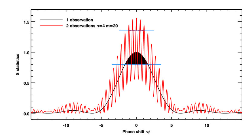
Figure 7.— Examples of the $S$ statistics for the period search (without the stochastic component) for one observation (black line) with a total exposure $T$ shown as black solid line and for two observations (red line) with exposure times $T_{1}=T$ and $T_{2}=T/4$ with the second observations starting at the moment $T_{s}=12T$. Shaded areas show examples of confidence regions: for the red curve it contains two secondary peaks on either side of the primary one.

A.3. Regularization of the pulse shape

We can improve the period search procedure by assuming the pulse shape to be smooth. This idea is similar to regularization techniques used in the image/signal reconstruction and therefore we can exploit similar mathematical methods. As long as the period is determined by searching the maximum of the $S$ statistics, we introduce the penalization factor that depends on the pulse shape $p(\phi)$ as:

$$S_{\mathrm{reg}}=S(1+k\int_{0}^{2\pi}(\frac{d^{2}p(\phi)}{d\phi^{2}})^{2}d\phi)^{1/2}$$ (A12)

Here $k$ is a positive coefficient that defines the degree of regularization. Numerically, the second derivative is computed for a discrete pulse shape as $\frac{3}{2}(box(p,3)-p)$ where $box(p,3)$ denotes the boxcar smoothing of the pulse $p$ with a window of 3 pixels.

Applying the regularization to real data results in much smoother pulse shapes while the periods always stay within the uncertainties predicted from the $S$ statistics or the analytic formulations provided above (Eq. A11). We stress that we do not smooth the actual pulse shape but rather bias the period search statistically towards smoother shapes. In Fig. 8 (left panel) we show an example of the recovered pulse shape from the dataset obtained in January of 2002 (ObsID: 0112570101) with and without regularization using $k=(2/3)^{2}$. The right panel shows the $S$ statistics without (blue) and with (green) regularization obtained from the folded epoch period search in 20 phase bins. Therefore, the $S$ statistics includes a stochastic contribution with the variance $<S_{\mathrm{rand}}>=19$. It is clear from the plot that the regularized solution lies within the $1\sigma$ confidence area, i.e. the period values are consistent within statistical uncertainties, however, the recovered pulse shape looks substantially smoother in the regularized case.

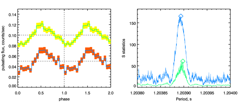
Figure 8.— The pulse profile recovered from the observation collected on 2002-01-06 (ObsID: 0112570101). (Left) The yellow and red lines are pulse shapes obtained with and without regularization respectively. (Right) The green and blue lines represent the S statistics versus spin period for the search with and without regularization respectively.

References

- Agar & Barmby (2013) Agar, J. R. R., & Barmby, P. 2013, AJ, 146, 135
- Alpar et al. (1982) Alpar, M. A., Cheng, A. F., Ruderman, M. A., & Shaham, J. 1982, Nature, 300, 728
- Archibald et al. (2009) Archibald, A. M., Stairs, I. H., Ransom, S. M., et al. 2009, Science, 324, 1411
- Arnaud (1996) Arnaud, K. A. 1996, in Astronomical Society of the Pacific Conference Series, Vol. 101, Astronomical Data Analysis Software and Systems V, ed. G. H. Jacoby & J. Barnes, 17
- Bachetti (2015) Bachetti, M. 2015, Astrophysics Source Code Library, record ascl:1502.021
- Bachetti et al. (2014) Bachetti, M., Harrison, F. A., Walton, D. J., et al. 2014, Nature, 514, 202
- Bahramian et al. (2014) Bahramian, A., Heinke, C. O., Sivakoff, G. R., et al. 2014, ApJ, 780, 127
- Baumgardt (2017) Baumgardt, H. 2017, MNRAS, 464, 2174
- Baumgardt et al. (2002) Baumgardt, H., Hut, P., & Heggie, D. C. 2002, MNRAS, 336, 1069
- Bekki & Freeman (2003) Bekki, K., & Freeman, K. C. 2003, MNRAS, 346, L11
- Bellini et al. (2013) Bellini, A., Piotto, G., Milone, A. P., et al. 2013, ApJ, 765, 32
- Bhattacharya & van den Heuvel (1991) Bhattacharya, D., & van den Heuvel, E. P. J. 1991, Phys. Rep., 203, 1
- Bhattacharya et al. (1992) Bhattacharya, D., Wijers, R. A. M. J., Hartman, J. W., & Verbunt, F. 1992, A&A, 254, 198
- Bildsten et al. (1997) Bildsten, L., Chakrabarty, D., Chiu, J., et al. 1997, ApJS, 113, 367
- Breton et al. (2007) Breton, R. P., Roberts, M. S. E., Ransom, S. M., et al. 2007, ApJ, 661, 1073
- Brown et al. (2016) Brown, T. M., Cassisi, S., D’Antona, F., et al. 2016, ApJ, 822, 44
- Buccheri et al. (1983) Buccheri, R., Bennett, K., Bignami, G. F., et al. 1983, A&A, 128, 245
- Caldwell et al. (2011) Caldwell, N., Schiavon, R., Morrison, H., Rose, J. A., & Harding, P. 2011, AJ, 141, 61
- Cavecchi et al. (2011) Cavecchi, Y., Patruno, A., Haskell, B., et al. 2011, ApJ, 740, L8
- Chakrabarty et al. (1997) Chakrabarty, D., Bildsten, L., Grunsfeld, J. M., et al. 1997, ApJ, 474, 414
- Chilingarian et al. (2009) Chilingarian, I., Cayatte, V., Revaz, Y., et al. 2009, Science, 326, 1379
- Chilingarian & Zolotukhin (2015) Chilingarian, I., & Zolotukhin, I. 2015, Science, 348, 418
- Chilingarian et al. (2011) Chilingarian, I. V., Mieske, S., Hilker, M., & Infante, L. 2011, MNRAS, 412, 1627
- Cohn et al. (2002) Cohn, H. N., Lugger, P. M., Grindlay, J. E., & Edmonds, P. D. 2002, ApJ, 571, 818
- Dabringhausen et al. (2012) Dabringhausen, J., Kroupa, P., Pflamm-Altenburg, J., & Mieske, S. 2012, ApJ, 747, 72
- Dickey & Lockman (1990) Dickey, J. M., & Lockman, F. J. 1990, ARA&A, 28, 215
- Drinkwater et al. (2003) Drinkwater, M. J., Gregg, M. D., Hilker, M., et al. 2003, Nature, 423, 519
- Eggleton (1983) Eggleton, P. P. 1983, ApJ, 268, 368
- Esposito et al. (2016) Esposito, P., Israel, G. L., Belfiore, A., et al. 2016, MNRAS, 457, L5
- Evans et al. (2010) Evans, I. N., Primini, F. A., Glotfelty, K. J., et al. 2010, ApJS, 189, 37
- Evstigneeva et al. (2008) Evstigneeva, E. A., Drinkwater, M. J., Peng, C. Y., et al. 2008, AJ, 136, 461
- Fabian et al. (1975) Fabian, A. C., Pringle, J. E., & Rees, M. J. 1975, MNRAS, 172, 15
- Faucher-Giguère & Kaspi (2006) Faucher-Giguère, C.-A., & Kaspi, V. M. 2006, ApJ, 643, 332
- Ferraro et al. (2009) Ferraro, F. R., Dalessandro, E., Mucciarelli, A., et al. 2009, Nature, 462, 483
- Francis et al. (2012) Francis, K. J., Drinkwater, M. J., Chilingarian, I. V., Bolt, A. M., & Firth, P. 2012, MNRAS, 425, 325
- Galleti et al. (2004) Galleti, S., Federici, L., Bellazzini, M., Fusi Pecci, F., & Macrina, S. 2004, A&A, 416, 917
- Ghosh & Lamb (1978) Ghosh, P., & Lamb, F. K. 1978, ApJ, 223, L83
- Gnedin et al. (2002) Gnedin, O. Y., Zhao, H., Pringle, J. E., et al. 2002, ApJ, 568, L23
- Harris (1996) Harris, W. E. 1996, AJ, 112, 1487
- Heinke et al. (2006) Heinke, C. O., Wijnands, R., Cohn, H. N., et al. 2006, ApJ, 651, 1098
- Hénon (1961) Hénon, M. 1961, Annales d’Astrophysique, 24, 369
- Heyl et al. (2015) Heyl, J., Richer, H. B., Antolini, E., et al. 2015, ApJ, 804, 53
- Hut et al. (1992) Hut, P., McMillan, S., Goodman, J., et al. 1992, PASP, 104, 981
- Ivanova et al. (2008) Ivanova, N., Heinke, C. O., Rasio, F. A., Belczynski, K., & Fregeau, J. M. 2008, MNRAS, 386, 553
- King & Lasota (2016) King, A., & Lasota, J.-P. 2016, arXiv, arXiv:1601.03738
- King (1966) King, I. R. 1966, AJ, 71, 64
- Krist et al. (2011) Krist, J. E., Hook, R. N., & Stoehr, F. 2011, in Society of Photo-Optical Instrumentation Engineers (SPIE) Conference Series, Vol. 8127, Society of Photo-Optical Instrumentation Engineers (SPIE) Conference Series, 0
- Kroupa (2002) Kroupa, P. 2002, Science, 295, 82
- Lanzoni et al. (2010) Lanzoni, B., Ferraro, F. R., Dalessandro, E., et al. 2010, ApJ, 717, 653
- Leahy (1987) Leahy, D. A. 1987, A&A, 180, 275
- Leahy et al. (1983) Leahy, D. A., Darbro, W., Elsner, R. F., et al. 1983, ApJ, 266, 160
- Lyne et al. (1993) Lyne, A. G., Biggs, J. D., Harrison, P. A., & Bailes, M. 1993, Nature, 361, 47
- Lyne et al. (1996) Lyne, A. G., Manchester, R. N., & D’Amico, N. 1996, ApJ, 460, L41
- Manchester et al. (2005) Manchester, R. N., Hobbs, G. B., Teoh, A., & Hobbs, M. 2005, AJ, 129, 1993
- Michel (1987) Michel, F. C. 1987, Nature, 329, 310
- Mushtukov et al. (2015) Mushtukov, A. A., Suleimanov, V. F., Tsygankov, S. S., & Poutanen, J. 2015, MNRAS, 447, 1847
- Narayan & Ostriker (1990) Narayan, R., & Ostriker, J. P. 1990, ApJ, 352, 222
- Olausen & Kaspi (2014) Olausen, S. A., & Kaspi, V. M. 2014, ApJS, 212, 6
- Osborne et al. (2001) Osborne, J. P., Borozdin, K. N., Trudolyubov, S. P., et al. 2001, A&A, 378, 800
- Papitto et al. (2011) Papitto, A., D’Aì, A., Motta, S., et al. 2011, A&A, 526, L3
- Patruno et al. (2012) Patruno, A., Alpar, M. A., van der Klis, M., & van den Heuvel, E. P. J. 2012, ApJ, 752, 33
- Patruno & Watts (2012) Patruno, A., & Watts, A. L. 2012, ArXiv e-prints, arXiv:1206.2727
- Peacock et al. (2010) Peacock, M. B., Maccarone, T. J., Knigge, C., et al. 2010, MNRAS, 402, 803
- Peng et al. (2002) Peng, C. Y., Ho, L. C., Impey, C. D., & Rix, H.-W. 2002, AJ, 124, 266
- Perna et al. (2006) Perna, R., Bozzo, E., & Stella, L. 2006, ApJ, 639, 363
- Pfeffer et al. (2014) Pfeffer, J., Griffen, B. F., Baumgardt, H., & Hilker, M. 2014, MNRAS, 444, 3670
- Podsiadlowski et al. (2002) Podsiadlowski, P., Rappaport, S., & Pfahl, E. D. 2002, ApJ, 565, 1107
- Pooley et al. (2003) Pooley, D., Lewin, W. H. G., Anderson, S. F., et al. 2003, ApJ, 591, L131
- Prager et al. (2016) Prager, B., Ransom, S., Freire, P., et al. 2016, ArXiv e-prints, arXiv:1612.04395
- Radhakrishnan & Srinivasan (1982) Radhakrishnan, V., & Srinivasan, G. 1982, Current Science, 51, 1096
- Ransom (2001) Ransom, S. M. 2001, PhD thesis, Harvard University
- Richstone & Tremaine (1986) Richstone, D. O., & Tremaine, S. 1986, AJ, 92, 72
- Riess et al. (2012) Riess, A. G., Fliri, J., & Valls-Gabaud, D. 2012, ApJ, 745, 156
- Rosen et al. (2015) Rosen, S. R., Webb, N. A., Watson, M. G., et al. 2015, ArXiv e-prints, arXiv:1504.07051
- Seth et al. (2014) Seth, A. C., van den Bosch, R., Mieske, S., et al. 2014, Nature, 513, 398
- Shaw Greening et al. (2009) Shaw Greening, L., Barnard, R., Kolb, U., Tonkin, C., & Osborne, J. P. 2009, A&A, 495, 733
- Siegel et al. (2007) Siegel, M. H., Dotter, A., Majewski, S. R., et al. 2007, ApJ, 667, L57
- Spitzer (1987) Spitzer, L. 1987, Dynamical evolution of globular clusters
- Spitzer & Hart (1971) Spitzer, Jr., L., & Hart, M. H. 1971, ApJ, 164, 399
- Strader et al. (2011) Strader, J., Caldwell, N., & Seth, A. C. 2011, AJ, 142, 8
- Supper et al. (2001) Supper, R., Hasinger, G., Lewin, W. H. G., et al. 2001, A&A, 373, 63
- Taylor (1992) Taylor, J. H. 1992, Philosophical Transactions: Physical Sciences and Engineering, 341, 117
- Trudolyubov et al. (2005) Trudolyubov, S., Kotov, O., Priedhorsky, W., Cordova, F., & Mason, K. 2005, ApJ, 634, 314