A Central Limit Theorem for Punctuated Equilibrium
K. Bartoszek
krzysztof.bartoszek@liu.se, krzbar@protonmail.ch,
Department of Computer and Information Science, Linköping University, 581 83 Linköping, Sweden
Abstract
Current evolutionary biology models usually assume that a phenotype undergoes
gradual change. This is in stark contrast to biological intuition, which
indicates that change can also be punctuated—the phenotype can jump.
Such a jump could especially occur at speciation, i.e. dramatic
change occurs that drives the species apart. Here we derive
a Central Limit Theorem for punctuated equilibrium. We show that,
if adaptation is fast, for weak convergence to normality to hold,
the variability in the occurrence of change has to disappear with time.
Keywords :
Branching diffusion process, Conditioned branching process,
Central Limit Theorem, Lévy process,
Punctuated equilibrium, Yule–Ornstein–Uhlenbeck with jumps process
A long–standing debate in evolutionary biology is whether
changes take place at times of speciation
(punctuated equilibrium Eldredge and Gould [28], Gould and Eldredge [32])
or gradually over time (phyletic gradualism, see references in Eldredge and Gould [28]).
Phyletic gradualism is in line with Darwin’s original envisioning of evolution
(Eldredge and Gould [28]).
On the other hand, the theory of punctuated equilibrium was an answer to what
fossil data was indicating (Eldredge and Gould [28], Gould and Eldredge [31, 32]).
A complete unbroken fossil series was rarely observed, rather
distinct forms separated by
long periods of stability (Eldredge and Gould [28]).
Darwin saw
“the fossil record more
as an embarrassment than as an aid to his theory” (Eldredge and Gould [28])
in the discussions with Falconer at the birth of the theory of evolution.
Evolution with jumps was proposed
under the name “quantum evolution” (Simpson [50]) to the scientific community.
However, only later (Eldredge and Gould [28]) was punctuated equilibrium re–introduced
into contemporary mainstream evolutionary theory.
Mathematical modelling of punctuated evolution on phylogenetic trees
seems to be still in its infancy
(but see Bokma [19, 21, 22], Mattila and Bokma [37], Mooers and Schluter [42], Mooers et al. [43]).
The main reason is that we do not seem to have sufficient understanding
of the stochastic properties of these models.
An attempt was made in this direction (Bartoszek [10])—to derive the tips’ mean,
variance, covariance and interspecies correlation for a branching
Ornstein–Uhlenbeck (OU) process with jumps at speciation, alongside
a way of quantitatively
assessing the effect of both types of evolution.
Very recently Bastide et al. [15] considered the problem
from a statistical point of view and proposed an Expectation–Maximization
algorithm for a phylogenetic Brownian motion with jumps
and OU with jumps in the drift function model. This work
is very important to indicate as it includes estimation software
for a punctuated equilibrium model, something not readily available earlier.
Bitseki Penda et al. [18] also recently looked into estimation
procedures for bifurcating Markov chains.
Combining jumps with an OU process is attractive
from a biological point of view. It is consistent with the
original motivation behind punctuated equilibrium.
At branching, dramatic events occur that drive species
apart. But then stasis between these jumps
does not mean that no change takes place, rather
that during it “fluctuations of little or no accumulated consequence” occur (Gould and Eldredge [32]).
The OU process fits into this idea because
if the adaptation rate is large enough, then the process reaches stationarity
very quickly and oscillates around the optimal state.
This then can be interpreted as stasis between the jumps—the small
fluctuations.
Mayr [38] supports this sort of reasoning by hypothesizing that
“The further removed in time a species from the original speciation
event that originated it, the more its genotype will
have become stabilized and the more it is likely to resist change.”
It should perhaps be noted at this point, that a Reviewer pointed out that the modelling
approach presented in this work is not the same as the “classical
view of punctuated equilibrium”. One would expect the jump to take place
in the direction of the optimum trait value. However, here at speciation
the jump is allowed to take place in any direction, also away from the optimum.
Then, after the jump, a relaxation period occurs and the trait
is allowed to evolve back to the optimum. Such a view on the jumps
is similar to e.g. Bokma [19, 21]’s modelling approach, however, there
the Brownian motion (BM) process was considered so no optimum parameter was present.
All the presented here results, concern the balance between the relaxation phenomena
and the jumps’ magnitudes and chances of occurring. One way of maybe thinking
about jumps going against the optimum, is that at the speciation event
a short–lived (as afterwords evolution goes again in the direction
of the previous optimum), random environmental niche appeared that allowed part of the species’
population to break–off and form a new species. However, to make this any more formal
one would have to link it with models for the environment, fitness and trait
dependent speciation, which is beyond the scope of this paper.
In this work we build up on previous results (Bartoszek [10], Bartoszek and Sagitov [12]) and
study in detail the asymptotic behaviour of the average of the tip
values of a branching OU process, with jumps at speciation points,
evolving on a pure birth tree.
To the best of our knowledge the work here is one of the
first to consider the effect of jumps on a
branching OU process in a phylogenetic context (but also look at Bastide et al. [15]).
It is possible that some of the results could be special
subcases of general results on branching Markov
processes (e.g. Abraham and Delmas [1], Bansaye et al. [8], Cloez and Hairer [24], Marguet [36], Ren et al. [46, 47, 48]).
However, these studies use a very heavy functional analysis
apparatus, which unlike the direct one here,
could be difficult for the applied reader. Bansaye et al. [8], Guyon [33], Bitseki Penda et al. [17]’s works
are worth pointing out as they connect their results on bifurcating Markov processes
with biological settings where branching phenomena are applicable, e.g. cell growth.
In the work here we can observe the (well known)
competition between the tree’s speciation and OU’s adaptation (drift)
rates, resulting in a phase transition when the latter is half the former
(the same as in the no jumps case
Adamczak and Miłoś [2, 3], Ané et al. [4], Bartoszek and Sagitov [12]).
We show here that if variability in jump occurrences disappears with time
or the model is in the critical regime (plus a bound assumption on the jumps’ magnitude and chances of occurring),
then the contemporary sample mean will be asymptotically normally distributed. Otherwise
the weak limit can be characterized as a “normal distribution with a
random variance”. Such probabilistic characterizations are important
as tools for punctuated phylogenetic models are starting to be developed
(e.g. Bastide et al. [15]).
This is partially due to an uncertainty of what is estimable, especially
whether the contribution of gradual and punctuated change
may be disentangled (but Bokma [22] indicates that they should be distinguishable).
Large sample size distributional approximations will allow for choosing seeds
for numerical maximum likelihood procedures and sanity checks if the results of numerical
procedures make sense. For example in the one–dimensional OU case it is known that (for a Yule tree)
the sample average is a consistent estimator of the long term mean and the sample variance of
the OU process’ stationary variance (Bartoszek and Sagitov [12]). In the BM (Yule tree) case one can have
a consistent estimator of the diffusion coefficient [13].
Hence, from these sample statistics one can construct starting values for numerical estimation
procedures (as e.g. mvSLOUCH does now, [14]).
Often a key ingredient in studying branching Markov processes is a
“Many–to–One” formula—the law of the trait
of an uniformly sampled individual in an “average” population (e.g. Marguet [36]). The approach
in this paper is that on the one hand we condition
on the population size, , but then to obtain the law (and its limit) of the contemporary
population, we consider moments of uniformly sampled species and the covariance between a
uniformly sampled pair of species.
The strategy to study the limit behaviour is to first condition
on a realization of the Yule tree and jump pattern (on which branches after speciation did the jump
take place). This is, as
conditional on the phylogeny and jump locations, the collection of the contemporary tips’ trait values
will have a multivariate normal distribution, and hence their sample average will be normally distributed.
We are able to represent (under the above conditioning) the variance of the sample average in terms of
transformations of the number of speciation events on randomly selected lineage,
time to coalescent of randomly selected pair of tips
and the number of common speciation events for a randomly selected pair of tips.
We consider the conditional (on the tree and jump pattern) expectation
of these transformations and then look at the rate of decay to
of the variances of these conditional expectations. If this rate of decay
is fast enough, then they will converge to a constant and
the normality of an appropriately scaled average of tips species will be retained in the limit.
Very briefly this rate of decay depends on how the product of the probability and variance
of the jump behaves along the nodes of the tree. We do not necessarily
assume (as previously in Bartoszek [10]) that the jumps are homogeneous on the whole tree.
First, in Section 2 we provide a series of formal definitions
that introduce key random variables associated with the phylogeny
that are necessary for this study.
Afterwords, in Section 3 we introduce the considered probabilistic model
and the concepts from Section 2 in a more intuitive manner.
Then, in Section 4 we present the main results. Section
5 is devoted to a series of technical convergence lemmata that
characterize the speed of decay of the effect of jumps
on the variance and covariance of tip species. Finally, in Section 6
we calculate the first two moments of a scaled sample average,
introduce a particular random variable related to the model and put this
together with the previous convergence lemmata to prove the
Central Limit Theorems (CLTs) of this paper.
It should be acknowledged at this point that
in the original arXiv preprint of this paper the convergence
to normality results were stated in an incomplete manner.
In particular the limiting normality in the critical regime was not described correctly.
The current characterization was noticed during the
collaboration with Torkel Erhardsson [11] and
more details on the previous mischaracterization can be found in Remark 4.7.
2 Notation
We first introduce two separate labellings for the tip and internal nodes
of the tree. Let the origin of the tree have label “”.
Next we label from “” to “” the internal nodes
of the tree in their temporal order of appearance. The root
is “”, the node corresponding to the second speciation event
is “” and so on. We label the tips of the
tree from “” to “” in an arbitrary fashion.
This double usage of the numbers “” to “”
does not generate any confusion as it will always
be clear whether one refers to a tip or internal node.
Definition 2.1
Definition 2.2
where denotes the cardinality of set .
Definition 2.3
For ,
Definition 2.4
For , define the finite sequence of length
as
Definition 2.5
For and ,
let be a binary random variable such that
where the should be understood in the natural way that there exists a position
in the sequence s.t. .
Definition 2.6
For and ,
let be a binary random variable equalling
iff a jump (an event that will be discussed in more detail Section 3)
took place just after the –th speciation event
in the sequence .
Definition 2.7
For and ,
let be a binary random variable equalling
iff and
, where .
Definition 2.8
For ,
where for two sequences and we define the operation
or in other words is the common prefix of sequences and .
Definition 2.9
For ,
where for a finite sequence , means its length.
Remark 2.10
We have the in the above definition of as we are interested
in counting the speciation events that could have a jump common to both lineages.
As the jump occurs after a speciation event, the jumps connected to the coalescent
node of tip nodes and cannot affect both of these tips (see Section 3.2).
Definition 2.11
For and ,
let be a binary random variable such that
For a sequence , the operation chooses the maximum value present in the sequence.
Definition 2.12
For ,
Definition 2.13
For and ,
let be a binary random variable equalling
iff and .
Definition 2.14
For and ,
let be a binary random variable equalling
iff and .
Definition 2.15
Let be uniformly distributed on and
be uniformly distributed on the set of ordered pairs
drawn from (i.e. ,
for )
Some of the variables defined in Defn. 2.15 are illustrated in Figs. 1, 5
and further described in the captions. It might be also useful to refer to Bartoszek [10], especially
Fig. A., therein.
Remark 2.16
For the sequences , ,
, , ,
the –th element is naturally indicated as
, , ,
, ,
respectively.
Remark 2.17
We drop the in the superscript for the random variables
, , , ,
and as their distribution will not depend
on (see Lemma 3.1 Section 3). In fact, in principle, there will be
no need to distinguish between
the version with and without the tilde. However, such a
distinction will make it more clear to what one is referring to in the subsequent derivations
in this work.
3 A model for punctuated stabilizing selection
3.1 Phenotype model
Stochastic differential equations (SDEs) are today the standard language to
model continuous traits evolving on a phylogenetic tree. The general
framework is that of a diffusion process
(1)
The trait, , follows Eq. (1) along each branch
of the tree (with possibly branch specific parameters).
At speciation times
this process divides into two processes evolving independently from that point.
A workhorse of contemporary phylogenetic comparative methods (PCMs) is the OU process
(2)
where sometimes the parameters , , are
allowed to vary over the tree
(see e.g. Bartoszek et al. [14], Beaulieu et al. [16], Butler and King [23], Hansen [34], Mitov et al. [41, 40]).
Without loss of generality, for the purpose of the results here, we could have taken .
However, we choose to retain the parameter for consistency with previous literature.
In this work we keep all the parameters (, , ) identical over the whole tree.
The probabilistic properties (e.g. B. de Saporta and Yao [7])
and statistical procedures (e.g. Azaïs et al. [6])
for processes with jumps have of course been developed.
In the phylogenetic context
there have been a few attempts to go beyond the diffusion framework
into Lévy process, including Laplace motion,
(Bartoszek [9], Duchen et al. [26], Landis et al. [35])
and jumps at speciation points (Bartoszek [10], Bastide et al. [15], Bokma [20, 21]).
We follow in the spirit of the latter
and consider that just after a branching point, with a probability
, independently on each daughter lineage, a jump can occur.
It is worth underlining here a key difference of this model from the one
considered by Bastide et al. [15]. Here after speciation
each daughter lineage may with probability jump (independently of the other).
In Bastide et al. [15]’s model, in the OU case,
the jump is not in the trait value but in the drift function, of Eq. (2).
We assume that the jump random variable, added to the trait’s value, is normally distributed with mean
and variance . In other words, if at time there
is a speciation event, then just after it, independently for each daughter lineage, the trait
process will be
(3)
where means the value of respectively just before and
after time , is a binary random variable with probability of being
(i.e. jump occurs) and .
The parameters and can, in particular, differ between speciation events.
Taking or we recover the YOU without jumps model and results
[described by 12].
3.2 The branching phenotype
In this work we consider a fundamental model of phylogenetic tree growth — the
conditioned on number of tip species pure birth process (Yule tree).
We first make the notation from Section 2 more intuitive,
illustrating it also in Figs. 1 and 5
(see also Bartoszek [10], Bartoszek and Sagitov [12], Sagitov and Bartoszek [49]).
We consider a tree that has tip species.
Let be the tree height, the time from today
(backwards) to the coalescent of a pair of randomly chosen tip species,
the time to coalescent of tips , ,
the number of speciation events on a random lineage,
the number of common speciation events for a
random pair of tips minus one
and
the number of common speciation events for
tips , minus one.
The jumps take place after the speciation event so
any jump associated with the speciation event that
split the two lineages, e.g. in Fig. 1
speciation event for the pair of lineages and ,
cannot be common to the the two lineages. Hence, in the
caption Fig. 1, we have
, see also Remark 2.10.
Furthermore, let be the sequence of nodes on a randomly chosen
lineage and be a binary sequence indicating if a jump took
place after each respective node in the sequence.
Finally, let be the time
between speciation events and ,
and be respectively the probability
and variance of the jump just after the –th speciation event
on each daughter lineage. It is worth recalling that (unlike in Bastide et al. [15]’s model)
both daughter lineages may jump independently of each other. It is also
worth reminding the reader that previously (in Bartoszek [10])
the jumps were homogeneous over the tree, in this manuscript
we allow their properties to vary with the nodes of the tree.
The following simple, yet very powerful, lemma
comes from the uniformity of the choice of pair to coalesce at the –th
speciation event in the backward description of the Yule process. The
proof can be found in Bartoszek [10] on p. (by no means do I claim this well known result as my own).
Lemma 3.1
Consider for a Yule tree the indicator random variables that the –th (counting from the root)
speciation event lies on a randomly selected lineage and
that the –th speciation event lies on the path from the origin to
the most recent common ancestor of a randomly selected pair of tips.
Then for all
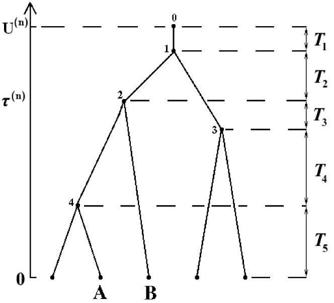
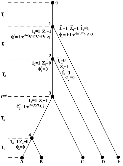
Figure 1:
A pure–birth tree with the various time components marked on it.
If we “randomly sample” node “A”, then and
the indexes of the speciation events on this random lineage are
,
and .
Notice that
always.
The between speciation times on this lineage are
, , and .
If we “randomly sample” the pair of extant
species “A” and “B”, then and the two nodes coalesced at time
.
The random index of their joint speciation event is
.
See also Fig. 5 and Bartoszek [10]’s Fig. A.. for a more detailed discussion on relevant notation.
The internal node labellings – are marked on the tree. The OUj process
evolves along the branches of the tree and we only observe the trait
values at the tips. For given tip, say “A” the value of the trait process
will be denoted . Of course here .
We called the model a conditioned one.
By conditioning we consider stopping the tree growth just before
the species occurs, or just before the –th speciation event.
Therefore, the tree’s height is a random stopping time.
The asymptotics considered in this work are when .
The key model parameter describing the tree component is , the birth rate. At the start,
the process starts with a single particle and then splits with rate .
Its descendants behave in the same manner. Without loss
generality we take , as this is equivalent to rescaling time.
In the context of phylogenetic
methods this branching process has been intensively studied
(e.g. Bartoszek and Sagitov [12], Crawford and Suchard [25], Edwards [27], Gernhard [29, 30], Mulder and Crawford [44], Sagitov and Bartoszek [49], Steel and McKenzie [53]),
hence here we will just describe its key property.
The time between speciation events and is exponential with
parameter . This is immediate from the memoryless
property of the process and the distribution of the minimum
of i.i.d. exponential random variables. From this we obtain some important
properties of the process.
Let be the –th harmonic number, and
then their expectations and Laplace transforms are (Bartoszek and Sagitov [12], Sagitov and Bartoszek [49])
where
being the gamma function.
Now let be the –algebra that
contains information on the Yule tree and jump pattern.
By this we mean that conditional on
we know exactly how the tree looks like (esp. the interspeciation times )
and we know at what parts of the tree (at which lineage(s) just after which speciation
events) did jumps take place. The motivation behind such conditioning is that
conditional on the contemporary tips sample is a multivariate normal one.
When one does not condition on the normality does not hold—the randomness
in the tree and presence/absence of jumps distorts normality.
Bartoszek [10] previously studied
the branching Ornstein–Uhlenbeck with jumps (OUj) model
and it was shown
(but, therein for constant and and
therefore there was no need to condition on the jump pattern) that,
conditional on the tree height and number of tip species
the mean and variance of the trait value of tip species (out of the contemporary),
(see also Fig. 1), are
(4)
, and are realizations
of the random variables , and when lineage is picked.
A key difference that the phylogeny brings in, is that the tip measurements
are correlated through the tree structure. One can easily show that conditional on ,
the covariance
between traits belonging to tip species and , and is
(5)
where , correspond to
the realization of random variables , , but
reduced to the common part of lineages and ,
while ,
correspond to realizations of ,
when the pair is picked.
We will call, the considered model the
Yule–Ornstein–Uhlenbeck with jumps (YOUj) process.
Remark 3.2
Keeping the parameter
constant on the tree is not as simplifying as it might seem. Varying
models have been considered since the introduction of the OU process
to phylogenetic methods (Hansen [34]). However, it can very often happen
that the parameter is constant over whole clades, as these
species share a common optimum due to some common discrete characteristic. Therefore, understanding the model’s
behaviour with a constant is a crucial first step.
Furthermore, if constant clades are apart far enough
one could think of them as independent samples
and attempt to construct a test (based on normality of the species’ averages)
if jumps have a significant effect
(compare Thms. 4.1 and 4.6).
For this one would have to make the very difficult to biologically justify
assumption of constant model parameters between clades. Though, one can imagine
special situations where the levels of are connected to a discrete
characteristic common to many clades, e.g. fresh water or seawater.
On the other hand CLTs and other asymptotical results for changing model
parameters and different levels of are an exciting
future research direction.
Remark 3.3
It should be noted that the phylogeny could be introduced using
a formal branching process approach and the
offspring’s’ generating function (e.g. Ch. III.3, Athreya and Ney [5]).
Then, the branching trait model can be described (jointly with the tree)
as a “Markov process in the space of integer–valued measures on ”
(Adamczak and Miłoś [3]). However, in this work here we do not use any of the
machinery from that direction and so we refrain from defining the setup in that language
so as to avoid adding yet another layer of notation. On the other hand, the way of defining
the model used here is constructive—in the sense that it can be directly coded in
a simulation procedure.
3.3 Martingale formulation
Our main aim is to study the asymptotic behaviour of the sample average and
it actually turns out to be easier to work with scaled trait values, for
each ,
Denoting
we have
(6)
The initial condition of course will be .
Remark 3.4
We remark, that here it becomes evident that the specific value of , will
not play any role in obtaining the presented here results. What only matters is the
initial displacement from , but even this will not contribute in any way
to the rate of convergence, only as a scaling constant for the
expectation of
(see Proof of Thm. 4.1).
Just as was done by Bartoszek and Sagitov [12]
we may construct a martingale related to the average
It is worth pointing out that is observed just before the –th
speciation event. An alternative formulation would be to observe it just after
the –st speciation event.
Then (cf. Lemma of Bartoszek and Sagitov [12]), we define
This is a martingale with respect to , the –algebra
containing information on the Yule –tree and the phenotype’s evolution,
i.e. .
4 Asymptotic regimes — main results
Branching Ornstein–Uhlenbeck models commonly have three asymptotic regimes
(Adamczak and Miłoś [2, 3], Ané et al. [4], Bartoszek [10], Bartoszek and Sagitov [12], Ren et al. [46, 47]).
The dependency between the adaptation rate
and branching rate governs in which regime the process is.
If , then the contemporary sample is similar to an i.i.d. sample,
in the critical case, , we can, after appropriate rescaling,
still recover the “near” i.i.d. behaviour
and if , then the process has “long memory”
(“local correlations dominate over the OU’s ergodic properties”, Adamczak and Miłoś [2, 3]).
In the context considered here by “near” and “similar” to i.i.d. we mean that the resulting CLTs resemble those
of an i.i.d. sample. For example the limit distribution of the normalized sample average
in the YOU regime [Thm. in 12] is
and taking
we obtain the classical limit (as intuition
could suggest with instantaneous adaptation).
In the YOUj setup the same three asymptotic regimes can be observed, even though
Adamczak and Miłoś [2, 3], Ren et al. [46, 47]
assume that
the tree is observed at a given time point, ,
with being random. In what follows here,
the constant may change between (in)equalities. It may in particular depend on
. We illustrate the below Theorems in Fig. 2.
We consider the process
which is the the normalized sample mean of the YOUj process with .
The next two Theorems consider its,
depending on , asymptotic with behaviour.
Theorem 4.1
Assume that the jump probabilities and jump variances are constant equalling and
respectively.
(I)
If and ,
then the conditional variance of the scaled sample mean
converges in to a finite mean and variance random variable .
The scaled sample mean,
converges weakly to random variable
whose characteristic function can be expressed in terms of the Laplace transform of
(II)
If ,
then is asymptotically normally distributed with mean and
variance .
In particular the conditional variance of the scaled sample mean
converges in (and hence in ) to the constant .
(III)
If , then converges almost surely and in to a random variable
with finite first two moments.
Remark 4.2
For the a.s. and convergence to hold in Part (III), it suffices that the
sequence of jump variances is bounded.
Of course, the first two moments will differ if the jump variance is not constant.
Remark 4.3
After this remark we will define the concept of a sequence converging to
with density . Should the reader find it easier, they may forget that the
sequence converges with density , but think of the sequence simply
converging to . The condition of convergence with density is
a technicality that through ergodic theory allows us to slightly
weaken the assumptions of the theorem that gives a normal limit.
Definition 4.4
A subset of
positive integers is said to have density (e.g. Petersen [45]) if
where is the indicator function of the set .
Definition 4.5
A sequence converges to with density if
there exists a subset of
density such that
Theorem 4.6
Assume that the sequence is bounded.
Then, depending on the process has the following
asymptotic with behaviour.
(I)
If ,
goes to with density
and the sequences , are such that
the sequences of expectations
converge, then the process is asymptotically normally distributed with mean and
variance .
(II)
If ,
and the sequences , are such that
the sequence of expectations
converges,
then is asymptotically normally distributed with mean and
variance .
It is worth pointing out that Thm. 4.6 covers the extreme cases and .
The convergence conditions on the expectations look rather daunting, however they will
simplify very compactly if and are constant or
(with density ). These we discuss after the proof of the theorem,
when we also mention why the assumptions on these expectations are necessary.
Remark 4.7
In the original arXiv preprint of this paper it was stated that convergence to normality
in the regimes will only take place if
is bounded and goes to with density .
Normality in the and regimes was noticed thanks
to the collaboration with Torkel Erhardsson
[11] and then, the results and proofs in this manuscript
were adjusted.
Remark 4.8
The assumption with density
is an essential one for the limit to be a normal distribution, when . This is
visible from the proof of Lemma 5.5. In fact, this is the
key difference that the jumps bring in—if their magnitude or
their uncertainty in occurrence is too large, then they will disrupt the weak convergence.
One possible way of achieving the above condition is to keep constant and allow ,
the chance of jumping becomes smaller relative to the number of species.
Alternatively, , which could
mean that with more and more species—smaller and smaller jumps occur at speciation.
Actually, one could intuitively think of this as biologically more realistic.
We are in the Yule, no extinction, case so with time there will be more and
more species (species here can be understood, if it helps intuition
as non–mixing, for some reason, populations). If they all live in some
spatially confined area, then as the number of species grows
there could be more and more competition. If one considers a trait
that is related to what is competed for, then
smaller and smaller differences
in phenotype could drive the species apart. Specialization occurs and tinier
and tinier niches are filled.
This reasoning of course
further assumes that the number of individuals grows with the number
of species. Furthermore, under the considered YOUj model the long time mean, , is the same
for all species, so even though there is an initial displacement
(into a different niche) with time the trait will try to revert to its optimum.
Hence, the above is not aiming for making any authoritative biological
statements, nor provide an interpretation of the whole YOUj model. Rather,
it has as its goal of giving some intuition on jump variance decreasing to
with time/number of species.
Remark 4.9
In Thm. 4.6 we do not consider the “fast branching/slow adaptation”,
regime. By assuming with density , it is possible
to make the influence of the jumps disappear asymptotically, just like in the case,
see Example 6.6. However, no further insights, than those in Thm. 4.1
will be readily available, similarly as Bartoszek and Sagitov [12] note for the YOU without jumps model. This
is as the used here methods, do not seem to easily extend
to the situation, beyond what is presented in this manuscript.
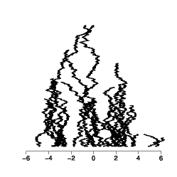
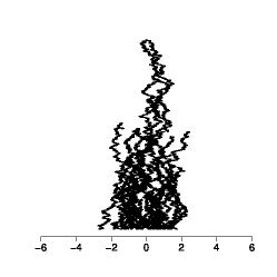
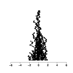
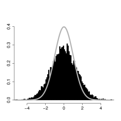
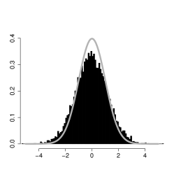
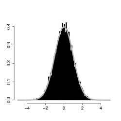
Figure 2:
Left: centre: and right: .
Top row: examples of simulated YOUj process trajectories,
bottom row: histograms of sample averages,
left: scaled by ,
centre: scaled by ,
right: scaled by .
In all three cases, , , ,
. The phylogenetic trees are pure birth trees
with conditioned on number of tips, for the trajectory plots and
for the histograms.
The histograms are based on simulated trees.
The sample mean and variances of the scaled data in the histograms are
left: , centre: and right: .
The gray curve painted on the histograms is the standard normal distribution.
The phylogenies are simulated by the TreeSim R package
(Stadler [51, 52]) and simulations of phenotypic evolution and trajectory plots
are done by functions of the, available on CRAN, mvSLOUCH R package.
We can see that as decreases the sample
variance is further away from the asymptotical (after scaling) and the histogram from
normality (though when we should not expect normality). This is as with
smaller convergence is slower.
5 A series of technical lemmata
We will now prove a series of technical lemmata describing the asymptotics of
driving components of the considered YOUj process.
For two sequences , the notation
will mean that
with and
.
Notice that always
when is used a defined or undefined constant
is present within . The key property is that
the asymptotic behaviour with does not change
after the sign.
The general approach to proving these lemmata is related to that in the proof
of Bartoszek and Sagitov [12]’s Lemma .
What changes here is that we need to take into account
the effects of the jumps [which were not considered in 12].
However, we noticed that there is an error in the proof of
Bartoszek and Sagitov [12]’s Lemma . Hence, below for the convenience
of the reader, we do not only cite the lemma but also provide
the whole corrected proof. In Remark 5.2, following the proof,
we briefly point the problem in the original wrong proof and
explain why it does not influence the rest of
Bartoszek and Sagitov [12]’s results.
Proof
For a given realization of the Yule -tree we denote by and
two versions of that are independent conditional
on . In other words
and correspond to two
independent choices of pairs of tips out of available. Conditional
on all heights in the tree are known—the randomness
is only in the choice out of the pairs or equivalently sampling out of the
set of coalescent heights. We have,
Let be the probability that two randomly chosen tips coalesced at the –th speciation event.
We know that (cf. Stadler [51]’s proof of her Theorem 4.1, using for our
or Bartoszek and Sagitov [12]’s Lemma 1 for a more general statement)
Writing
and as the times between speciation events are independent and exponentially distributed
we obtain
On the other hand,
Taking the difference between the last two expressions we find
Noticing that we are dealing with a telescoping sum and hence using the relation
(8)
we see that it suffices to study the asymptotics of,
where
To consider these two asymptotic relations we observe that for large
Now since
,
it follows
and
Summarizing
Remark 5.2
Bartoszek and Sagitov [12]
wrongly stated in their Lemma that
for all .
From the above we can see that this holds only for . This does not however change
Bartoszek and Sagitov [12]’s main results.
If one inspects the proof of Theorem therein, then one can see
that for it is required that
,
where .
This by Lemma 5.1 holds. Bartoszek and Sagitov [12]’s Thm. does not depend on the rate of
convergence,
only that with .
This remains true, just with a different rate.
Let be the sequence of speciation events on a random lineage
and be the jump pattern (binary sequence jump took place, did not take place
just after speciation event )
on a randomly selected lineage.
Lemma 5.3
For random variables derived
from the same random lineage and
a fixed jump probability
we have
(9)
Proof
We introduce the random variables
and
where is the binary random variable if a jump took place at the –th speciation event
of the tree for our considered random lineage.
Obviously
Immediately (for )
We illustrate the random objects defined above in Fig. 5.
The term can be
expressed as
(same as with
in Lemma 5.1),
where and are two copies of
that are independent given ,
i.e. for a given tree we sample two lineages and ask if the –th speciation event
is on both of them. This will occur if these lineages coalesced at a speciation event
. Therefore,
Together with the above
Now
We notice that we are dealing with a telescoping sum, we take advantage of Eq. (8) again
and consider the three parts in turn.
(11)
Putting these together we obtain
On the other hand the variance is bounded from below by
5.
Its asymptotic behaviour is tight
as the calculations there are accurate up to a constant (independent of ).
This is further illustrated by graphs
in Fig. 3.
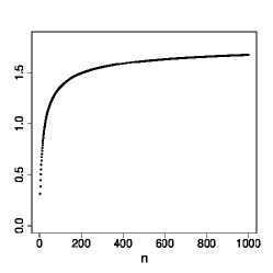
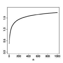
Figure 3: Numerical evaluation of scaled Eq. (5) for
different values of . The scaling for
left: equals ,
centre: equals
and right equals
In all cases, .
The value of the leading constant comes from a careful treatment
of the summation in Lemma 5.3.
The sums are approximated by definite integrals and the leading constant
resulting from the integration is remembered (in the panel on the right).
Corollary 5.4
Let and be respectively the jump probability and
variance at the –th speciation event, such that the sequence is bounded.
We have
iff with density .
Proof
We consider the case, .
Notice that in the proof of Lemma 5.3
.
If the jump probability and variance are not constant, but as in the Corollary, then
Notice that if with density , then so will
.
The Corollary is a consequence of a more general ergodic property, similar to Petersen [45]’s Lemma (p. ).
Namely take and if a bounded sequence
with density , then
To show this say the sequence is bounded by , let be
the set of natural numbers such that if and
define . Then
Denoting by the cardinality of a set ,
the former sum is bounded above by , which, by assumption,
tends to as . For the latter sum, given ,
if we choose such that for all and
such that for all ,
then for all , one has that
and now one has that the former sum is bounded above by
and the latter by . This proves the result.
On the other hand if does not go to with density , then
When we obtain the Corollary using the same ergodic argumentation for
Let be the sequence of speciation events on
the lineage from the origin of the tree to the most recent common ancestor
of a pair of randomly selected tips
and be the jump pattern
(binary sequence jump took place, did not take place just after speciation event )
on the lineage from the origin of the tree to the most recent common ancestor
of a pair of randomly selected tips.
Lemma 5.5
For random variables derived
from the same random pair of lineages and a fixed jump probability
(12)
Proof
We introduce the notation
and by definition we have
We introduce the random variable
where is the binary random variable if a jump took place just after the –th speciation event
of the tree for our considered lineage and obviously (for )
We illustrate the random objects defined above in Fig. 5.
We can write similarly (but not exactly the same) as for
As usual (just as for in Lemma 5.1)
let and
be two conditionally on independent copies of
and now
Writing out a product of two sums, for , as
and using the law of total probability to condition on the speciation event at which the two nodes
coalesced, we have
To aid intuition, we point out that cases 5 and 5 correspond to the case when
the two pairs of tips coalesce at the same node while cases 5–5
when at different nodes, .
We first observe
and
(14)
Using the above, we consider each of the five components in this sum separately.
The variance is bounded from below by
5 and as these derivations
are correct up to a constant (independent of )
the variance behaves as above. This is further illustrated by graphs
in Fig. 4.
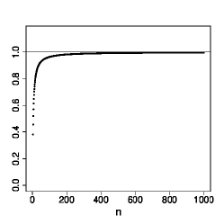
Figure 4:
Numerical evaluation of scaled Eq. (5) for
different values of . The scaling for
left: equals ,
centre: equals
and right equals
In all cases, .
The value of the leading constant comes from a careful treatment
of the summation in Lemma 5.5, component 5.
The sums (centre and right panel) are approximated by definite integrals and the leading constant
resulting from the integration is remembered. In the case the convergence is very slow.
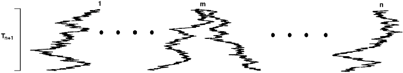
Figure 5:
Illustration of the key random variables used in
Lemmata 5.3, 5.5
and defined in Section 2.
We “randomly sample” (out of the five) the lineage leading to
tip A and the pair of tips (A,C) out of possible.
As jumps take place just after speciation events there
is no associated jump at the third speciation event for
the (A,C) pair. We have
as it would be one for three (A,B, or C) randomly
sampled lineages out of the five possible.
One should remember that for an OU process, , for
one has ,
hence all contributions of the jumps to the variance and covariance are modified by ,
where is the distance from the jump to the tip. Intuitively writing, the variable
will then be (for )
the contribution of the jumps to the variance of the randomly sampled lineage,
while will then be (for )
the contribution of the jumps to the variance of the randomly sampled lineage.
Remark 5.6
In Lemma 5.5 we assumed that . The case of
is trivial, as then for all , and hence the
variance will be . The case is more interesting. It means that there
will be a jump on each lineage after each speciation event. This however
implies that the variability due to the uncertainty, if a jump did or did not
take place, disappears. Hence, a faster rate of convergence will be present in
component 5. It will be for ,
for and for , i.e. same as in components
5, 5 and 5.
The proof of the next Corollary, 5.7,
is exactly the same as of Corollary 5.4.
Corollary 5.7
Let and be respectively the jump probability and
variance at the –th speciation event, such that the sequence is bounded.
We have
iff with density .
Lemma 5.8
For random variables ,
and a fixed jump probability
(15)
Proof
We introduce the random variable
and obviously
Writing out
(20)
Lemma 5.9
For random variables
and a fixed jump probability
(21)
Proof
We introduce the random variable for
and obviously
As in the proofs of previous lemmata we denote by and
realizations of and that are conditionally
independent given . In other words, given a particular Yule tree
and will correspond to two independent
choices of pairs of tip species.
In the below derivations will correspond to the node where the random pair,
connected to , coalesced and will correspond to the node where the random pair
coalesced. Notice that the conditional expectation of
given that the coalescent took place at node is
. Writing out
We may recognize that, after bounding from below
by appropriately , or ,
under the sums over we will have a difference corresponding
to a telescoping sum, i.e. Eq. (8).
This implies that the whole covariance must be positive.
Notice the similarity to the sums
present in Eqs. (11) and (14).
We also give intuition how all the individual sums arose. Component
5 corresponds to the case where both randomly sampled pairs coalesce at the
same node. Component 5 corresponds to the situation where the random pair
of tips associated with coalesced later (further away from the origin of the tree),
than the random pair associated with . Components 5 and
5 correspond to the opposite situation. In particular
component 5 is when the “” node on the path from the origin
to node “” is earlier than or at the same node as the coalescent associated with
and component 5 when later.
Remark 5.10
Notice that the proof of Lemma 5.9 can easily be continued, in the same fashion
as the proofs of Lemmata 5.1–5.8 to
find the rate of the decay to of .
However, in order not to further lengthen the technicalities we remain at showing the sign of the
covariance, as we require only this property.
To avoid unnecessary notation it will be always assumed
that under a given summation sign
the random variables are derived
from the same random lineage and
also are derived
from the same random pair of lineages
Lemma 6.1
Conditional on
the first two moments of the scaled sample average are
Proof
The first equality is immediate. The variance follows from
This immediately entails the second moment.
Before stating the next lemma we remind the reader of a key, for this manuscript, result presented in
Bartoszek [10]’s Appendix A. (top of second column, p. ) in the case of constant
(22)
Lemma 6.2
Assume that the jump probability is constant, equalling , at every speciation event.
Let
and then for all and greater than some
converges a.s. and in to a random variable
with expectation
In particular for (and also , see Remark 6.3)
is a constant and the convergence is a.s. and .
Prooffor
We know that
for some constant , as by Eq. (22).
Furthermore, by Lemma 5.5 , for some constant .
Looking in detail, one can see from Eq. (22),
that will (from large enough) converge monotonically to its limit.
It will be decreasing with for and increasing for .
If one considers the asymptotic behaviour, then
the leading term will be .
Direct calculations show that for it will be decreasing, as it behaves as
, for it will be increasing as it behaves as
, while for for it will be increasing as it behaves as
.
Therefore, if one studies the proof of the downcrossing inequality
and submartingale convergence theorem (e.g. Thm. , Cor. , p. , Medvegyev [39]) one
will notice that only the monotonicity (which in the classical submartingale convergence theorem is
a consequence of the sequence being a submartingale) and boundedness
of the expectations of the sequence of positive random variables are required for the
almost sure convergence. All of the above is met in our case for .
Hence, by the above a.s.
for some random variable and as all expectations are finite,
and the variance is uniformly bounded we have .
This entails
.
Also we have
uniform integrability of and hence convergence.
Proof for
By Lemma 5.5 we know that
behaves as . Therefore,
.
Therefore, converges a.s. and in to a constant .
Proof for
is the same as the proof for , except that
now the leading terms in the asymptotic behaviour of
will be
.
This causes the sequence of expectations to be increasing (from large enough) and we may
argue similar as when .
From Eq. (22)
we obtain and
is bounded by a constant by Lemma 5.5.
Remark 6.3
If , we are in the trivial case of no jumps. When , in regime
we will have converging a.s. and in to a constant, denoted above as
, by the same argument
that takes place for , i.e. as the rate of decay to of
is faster than .
In the regime the argumentation presented above
holds for and no convergence to a constant can be deduced, as Lemma 5.5
does not provide a different rate of decay of .
Remark 6.4
It is worth noticing that has a very interesting recursive structure.
Denote by the value that would
take if the randomly chosen pair of species would be tips and
and by the value that would
take if tip is sampled.
where is a binary random variable indicating whether it is the –th lineage that split
(see Fig. 6). It is worth emphasizing that the sum defining splits
according to whether one picks both members of the pair of species splitting in the last
speciation event or only one of them.
Figure 6: The situation of the process between the –th and –st split. Node split
so and for . The time between the splits is .
Obviously the distribution of the vector is uniform
on the –element set
. In particular note
Furthermore, shows resemblance to a martingale as the coefficient
converges to monotonically, depending on
from above or below, while
.
Proof of Theorem 4.1, Part (I), We will show convergence in probability of the conditional mean and variance
for a finite mean and variance random variable .
Then, due to the conditional normality of this will give the
convergence of
characteristic functions
and the desired weak convergence, i.e.
Using Lemma 6.1 and that the Laplace transform
of the average coalescent time [Lemma in 12] is
(23)
we can calculate
Therefore we have in and hence in .
Remembering that
was assumed constant, equalling ,
Lemma 6.1 states that
Remembering that was assumed constant, equalling ,
we know that
Putting these individual components together we obtain the convergence and hence
Proof of Part (III),
We notice that the martingale (with respect to )
has
uniformly bounded second moments. Namely by Lemma 6.1,
a modification of Lemma 5.8, Cauchy–Schwarz, bounding by a constant
and remembering that in this case is constant
To deal with one slightly modifies the proof
of Lemma 5.8. Namely instead of considering the random variable ,
consider
and then doing similar calculations one will obtain a decay of order .
It is also worth pointing out that using Bartoszek and Sagitov [12]’s Lemma 3
for a more detailed consideration of ,
would not result in a different rate of decay, than what Cauchy–Schwarz provides, i.e. .
Hence, and by the martingale convergence theorem,
a.s. and in .
We obtain
a.s. and in , where is the a.s. and limit of
(cf. Lemma 9 in Bartoszek and Sagitov [12]).
Notice that for the convergence to hold in the regime,
it is not required that
is constant, only bounded.
We may also obtain directly the first two moments of
(however, for these formulæ to hold, has to be constant)
From the proof of Part (I), Theorem 4.1
we know that in probability.
Then, by the assumptions of the theorem on the expectations
Furthermore, Lemma
5.3 (the sequence is bounded by assumption)
and Corollary 5.7 ( with density by assumption) imply
Therefore we obtain that in probability
and by convergence of characteristic functions
we obtain the asymptotic normality. Notice that on the other hand using
the Cauchy–Schwarz inequality, Lemmata 5.8 and 5.9
we obtain
where is some sequence decaying to with a rate depending on .
Assume now that does not converge with density .
Then, by Corollary 5.7 we will have
implying
and hence, the convergence of the characteristic functions as above does not hold.
Therefore, the convergence with density is
a necessary assumption for the asymptotic normality.
Proof of Part (II),
This is proved in the same way as Part (I).
Due to the boundedness of (implying is bounded)
and as before
Then, due to the assumption on the expectation we have that
as due to the boundedness of by Lemma 5.5
Remark 6.5
The boundedness assumption for (), together with the convergence to
with density of (for ) allows for controlling
. The boundedness assumption would still allow for showing that
is bounded but would not suffice for convergence. For example,
consider constant and for odd and for even.
Then, for we would have in probability
It does seem that for the assumption that is bounded
could be relaxed. However, it would essentially require that one explicitly
assumes that the sequences , are such that the
sequences of the variances of the conditional expectations converge to
(as was needed for the sequences of the expectations).
Example 6.6
Assume that with density .
Then,
by the same ergodic argument as in Corollary 5.4
and following the steps in the proof of Thm. 4.6
we obtain
that for we have
resulting in
and for we have also
resulting in
.
Hence, to recover [12]’s CLTs one needs the stronger
assumption of with density .
Acknowledgements
A significant part of this work was done at the Department of
Mathematics, Uppsala University, Sweden, during my postdoc which was supported
by the Knut and Alice Wallenberg Foundation. Currently I am supported by the
Swedish Research Council (Vetenskapsrådet) grant no. –.
I would like to acknowledge Olle Nerman for his suggestion on adding jumps to the
branching OU process, Wojciech Bartoszek for helpful suggestions concerning
ergodic arguments, Venelin Mitov and Tanja Stadler for many discussions.
I would like to thank anonymous reviewers who found a number of errors and
whose comments immensely improved the manuscript. I am especially grateful
for pointing out a number of flaws in the original proof
of Corollary 5.4 and suggesting a significantly more elegant way
of proving it. I am also grateful to Torkel Erhardsson and our collaboration
[11] which allowed for a correct formulation
of Thms. 4.1 and 4.6.
References
Abraham and Delmas [2012]
R. Abraham and J.-F. Delmas.
A continuum–tree–valued Markov process.
Ann. Appl. Probab., 40(3):1167–1211,
2012.
Adamczak and Miłoś [2014]
R. Adamczak and P. Miłoś.
U–statistics of Ornstein–Uhlenbeck branching particle system.
J. Th. Probab., 27(4):1071–1111, 2014.
Adamczak and Miłoś [2015]
R. Adamczak and P. Miłoś.
CLT for Ornstein–Uhlenbeck branching particle system.
Elect. J. Probab., 20(42):1–35, 2015.
Ané et al. [2017]
C. Ané, L. S. T. Ho, and S. Roch.
Phase transition on the convergence rate of parameter estimation
under an Ornstein–Uhlenbeck diffusion on a tree.
J. Math. Biol., 74:355–385, 2017.
Athreya and Ney [2004]
K. B. Athreya and P. E. Ney.
Branching Processes.
Dover Publications, New York, 2004.
Azaïs et al. [2014]
R. Azaïs, F. Dufour, and A. Gégout-Petit.
Non–parametric estimation of the conditional distribution of the
interjumping times for piecewise–deterministic Markov processes.
Scand. J. Stat., 41(4):950–969, 2014.
B. de Saporta and Yao [2005]
B. de Saporta and J.-F. Yao.
Tail of a linear diffusion with Markov switching.
Ann. Appl. Probab., 15(1B):992–1018,
2005.
Bansaye et al. [2011]
V. Bansaye, J.-F. Delmas, L. Marsalle, and V. C. Tran.
Limit theorems for Markov processes indexed by continuous time
Galton-–Watson trees.
Ann. Appl. Probab., 21(6):2263–2314,
2011.
Bartoszek [2012]
K. Bartoszek.
The Laplace motion in phylogenetic comparative methods.
In Proceedings of the Eighteenth National Conference on
Applications of Mathematics in Biology and Medicine, Krynica Morska, pages
25–30, 2012.
Bartoszek [2014]
K. Bartoszek.
Quantifying the effects of anagenetic and cladogenetic evolution.
Math. Biosci., 254:42–57, 2014.
Bartoszek and Erhardsson [2019]
K. Bartoszek and T. Erhardsson.
Normal approximation for mixtures of normal distributions and the
evolution of phenotypic traits.
ArXiv e-prints, 2019.
Bartoszek and Sagitov [2015a]
K. Bartoszek and S. Sagitov.
Phylogenetic confidence intervals for the optimal trait value.
J. App. Prob., 52:1115–1132, 2015a.
Bartoszek and Sagitov [2015b]
K. Bartoszek and S. Sagitov.
A consistent estimator of the evolutionary rate.
J. Theor. Biol., 371:69–78, 2015b.
Bartoszek et al. [2012]
K. Bartoszek, J. Pienaar, P. Mostad, S. Andersson, and T. F. Hansen.
A phylogenetic comparative method for studying multivariate
adaptation.
J. Theor. Biol., 314:204–215, 2012.
Bastide et al. [2017]
P. Bastide, M. Mariadassou, and S. Robin.
Detection of adaptive shifts on phylogenies by using shifted
stochastic processes on a tree.
J. R. Statist. Soc. B, 2017.
Beaulieu et al. [2012]
J. M. Beaulieu, D.-C. Jhwueng, C. Boettiger, and B. C. O’Meara.
Modeling stabilizing selection: Expanding the Ornstein–Uhlenbeck
model of adaptive evolution.
Evolution, 66:2369–2389, 2012.
Bitseki Penda et al. [2014]
S. V. Bitseki Penda, H. Djellout, and A. Guillin.
Deviation inequalities, moderate deviations and some limit theorems
for bifurcating Markov chains with application.
Ann. Appl. Probab., 24(1):235–291, 2014.
Bitseki Penda et al. [2017]
S. V. Bitseki Penda, M. Hoffmann, and A. Olivier.
Adaptive estimation for bifurcating Markov chains.
Bernoulli, 23(4B):3598–3637, 2017.
Bokma [2002]
F. Bokma.
Detection of punctuated equilibrium from molecular phylogenies.
J. Evol. Biol., 15:1048–1056, 2002.
Bokma [2003]
F. Bokma.
Testing for equal rates of cladogenesis in diverse taxa.
Evolution, 57(11):2469–2474, 2003.
Bokma [2008]
F. Bokma.
Detection of “punctuated equilibrium” by Bayesian estimation of
speciation and extinction rates, ancestral character states, and rates of
anagenetic and cladogenetic evolution on a molecular phylogeny.
Evolution, 62(11):2718–2726, 2008.
Bokma [2010]
F. Bokma.
Time, species and seperating their effects on trait variance in
clades.
Syst. Biol., 59(5):602–607, 2010.
Butler and King [2004]
M. A. Butler and A. A. King.
Phylogenetic comparative analysis: a modelling approach for adaptive
evolution.
Am. Nat., 164(6):683–695, 2004.
Cloez and Hairer [2015]
B. Cloez and M. Hairer.
Exponential ergodicity for Markov processes with random switching.
Bernoulli, 21(1):992–1018, 2015.
Crawford and Suchard [2013]
F. W. Crawford and M. A. Suchard.
Diversity, disparity, and evolutionary rate estimation for unresolved
Yule trees.
Syst. Biol., 62(3):439–455, 2013.
Duchen et al. [in press 2016]
P. Duchen, C. Leuenberger, S. M. Szilàgyi, L. Harmon, J. Eastman,
M. Schweizer, and D. Wegmann.
Inference of evolutionary jumps in large phylogenies using Lévy
processes.
Syst. Biol., in press 2016.
Edwards [1970]
A. W. F. Edwards.
Estimation of the branch points of a branching diffusion process.
J. Roy. Stat. Soc. B, 32(2):155–174,
1970.
Eldredge and Gould [1972]
N. Eldredge and S. J. Gould.
Punctuated equilibria: an alternative to phyletic gradualism.
In T. J. M. Schopf and J. M. Thomas, editors, Models in
Paleobiology, pages 82–115. Freeman Cooper, San Francisco, 1972.
Gernhard [2008a]
T. Gernhard.
The conditioned reconstructed process.
J. Theor. Biol., 253:769–778, 2008a.
Gernhard [2008b]
T. Gernhard.
New analytic results for speciation times in neutral models.
B. Math. Biol., 70:1082–1097, 2008b.
Gould and Eldredge [1977]
S. J. Gould and N. Eldredge.
Punctuated equilibria: the tempo and mode of evolution reconsidered.
Paleobiology, 3(2):115–151, 1977.
Gould and Eldredge [1993]
S. J. Gould and N. Eldredge.
Punctuated equilibrium comes of age.
Nature, 366:223–227, 1993.
Guyon [2007]
J. Guyon.
Limit theorems for bifurcating Markov chains. Application to the
detection of cellular aging.
Ann. Appl. Probab., 17(5/6):1538–1569,
2007.
Hansen [1997]
T. F. Hansen.
Stabilizing selection and the comparative analysis of adaptation.
Evolution, 51(5):1341–1351, 1997.
Landis et al. [2013]
M. J. Landis, J. G. Schraiber, and M. Liang.
Phylogenetic analysis using Lévy processes: finding jumps in the
evolution of continuous traits.
Syst. Biol., 62(2):193–204, 2013.
Marguet [2019]
A. Marguet.
Uniform sampling in a structured branching population.
Bernoulli, 25(4A):2649–2695, 2019.
Mattila and Bokma [2008]
T. M. Mattila and F. Bokma.
Extant mammal body masses suggest punctuated equilibrium.
Proc. R. Soc. B, 275:2195–2199, 2008.
Mayr [1982]
E. Mayr.
Speciation and macroevolution.
Evolution, 36:1192–1132, 1982.
Medvegyev [2007]
P. Medvegyev.
Stochastic Integration Theory.
Oxford University Press, Oxford, 2007.
Mitov et al. [2019]
V. Mitov, K. Bartoszek, and T. Stadler.
Automatic generation of evolutionary hypotheses using mixed
Gaussian phylogenetic models.
PNAS, pages 16921–16926, 2019.
Mitov et al. [2020]
V. Mitov, K. Bartoszek, G. Asimomitis, and T. Stadler.
Fast likelihood calculation for multivariate Gaussian phylogenetic
models with shifts.
Theor. Pop. Biol., 131:66–78, 2020.
Mooers and Schluter [1998]
A. Ø. Mooers and D. Schluter.
Fitting macroevolutionary models to phylogenies: an example using
vertebrate body sizes.
Contrib. Zool., 68:3–18, 1998.
Mooers et al. [1999]
A. Ø. Mooers, S. M. Vamosi, and D. Schluter.
Using phylogenies to test macroevolutionary hypotheses of trait
evolution in Cranes (Gruinae).
Am. Nat., 154:249–259, 1999.
Mulder and Crawford [2015]
W. H. Mulder and F. W. Crawford.
On the distribution of interspecies correlation for Markov models
of character evolution on Yule trees.
J. Theor. Biol., 364:275–283, 2015.
Petersen [1983]
K Petersen.
Ergodic Theory.
Cambridge University Press, Cambridge, 1983.
Ren et al. [2014]
Y.-X. Ren, R. Song, and R. Zhang.
Central limit theorems for supercritical branching Markov
processes.
J. Func. Anal., 266:1716–1756, 2014.
Ren et al. [2015]
Y.-X. Ren, R. Song, and R. Zhang.
Central limit theorems for supercritical superprocesses.
Stoch. Proc. Appl., 125:428–457, 2015.
Ren et al. [2017]
Y.-X. Ren, R. Song, and R. Zhang.
Central limit theorems for supercritical branching nonsymmetric
Markov processes.
Ann. Appl. Probab., 45(1):564–623, 2017.
Sagitov and Bartoszek [2012]
S. Sagitov and K. Bartoszek.
Interspecies correlation for neutrally evolving traits.
J. Theor. Biol., 309:11–19, 2012.
Simpson [1947]
G. G. Simpson.
Tempo and mode in evolution.
Columbia University Press, New York, 1947.
Stadler [2009]
T. Stadler.
On incomplete sampling under birth-death models and connections to
the sampling-based coalescent.
J. Theor. Biol., 261(1):58–68, 2009.
Stadler [2011]
T. Stadler.
Simulating trees with a fixed number of extant species.
Syst. Biol., 60(5):676–684, 2011.
Steel and McKenzie [2001]
M. Steel and A. McKenzie.
Properties of phylogenetic trees generated by Yule–type speciation
models.
Math. Biosci., 170:91–112, 2001.