Optimal enzyme rhythms in cells

Abstract

Cells can use periodic enzyme activities to adapt to periodic environments or existing internal rhythms and to establish metabolic cycles that schedule biochemical processes in time. A periodically changing allocation of the protein budget between reactions or pathways may increase the overall metabolic efficiency. To study this hypothesis, I quantify the possible benefits of small-amplitude enzyme rhythms in kinetic models. Starting from an enzyme-optimised steady state, I score the effects of possible enzyme rhythms on a metabolic objective and optimise their amplitudes and phase shifts. Assuming small-amplitude rhythms around an optimal reference state, optimal phases and amplitudes can be computed by solving a quadratic optimality problem. In models without amplitude constraints, general periodic enzyme profiles can be obtained by Fourier synthesis. The theory of optimal enzyme rhythms combines the dynamics and economics of metabolic systems and explains how optimal small-amplitude enzyme profiles are shaped by network structure, kinetics, external rhythms, and the metabolic objective. The formulae show how orchestrated enzyme rhythms can exploit synergy effects to improve metabolic performance and that optimal enzyme profiles are not simply adapted to existing metabolic rhythms, but that they actively shape these rhythms to improve their own (and other enzymes’) efficiency. The resulting optimal enzyme profiles “portray” the enzymes’ dynamic effects in the network: for example, enzymes that act synergistically may be coexpressed, periodically and with some optimal phase shifts. The theory yields optimality conditions for enzyme rhythms in metabolic cycles, with static enzyme adaptation as a special case, and predicts how cells should combine transcriptional and posttranslational regulation to realise enzyme rhythms at different frequencies.

Keywords: Metabolic oscillation, metabolic control theory, optimal control, enzyme oscillation, periodic synergy, allosynchrony, pattern formation

1 Introduction

The lives of organisms are shaped by biological rhythms such as sleep rhythms or seasonal flowering. By adapting to daily or yearly rhythms in the environment, organisms can perform actions when conditions are best, and can anticipate changes, e.g. producing storage compounds for the night or winter times. Other rhythms like heart beat, breathing, or menstrual cycle emerge spontaneously. There are also rhythms within cells (e.g. the cell division cycle or circadian photosynthesis [1]) and specifically in metabolism [2, 3], as widely visible in gene expression data. Yeast cells show autonomous metabolic oscillations that involve genome-wide periodic gene expression [4, 5], as well as periodic production, storage, and consumption of metabolites. These oscillations also exist in single cells [6], and cell populations may auto-synchronise to show joint oscillations [7] in which cells adapt to varying conditions created by the entire cell population. They involve large parts of the transcriptome, with different functional subsystems peaking in different phases. Expression oscillations accompany both “outside” changes like day-night cycles or cell cycle and “internal” oscillations like to repiratory or metabolic cycles in yeast, which appear to be autonomous, but possibly synchronised with other cycles.

While mechanisms behind biochemical oscillations [8] and the molecular regulators of genome-wide expression oscillations have been thoroughly studied, their functions are still debated. Metabolic oscillations may be a side effect of dynamics, for example of overshooting gene regulation, but they may also have specific functions – in other words: they may provide benefits. It has been claimed that “pumping”, i.e. periodic concentration and flux changes, can increase the efficiency of biochemical pathways [9, 10]. More generally, metabolic cycles may allow cells to arrange their metabolic processes in time and across the entire metabolic network to optimise the resource usage [3]: mutually incompatible processes may be run at different times to avoid adverse effects, while other biochemical processes may run in “concerted actions” or in a favourable temporal order. The yeast metabolic cycle shows a characteristic sequence of physiological phases that functionally build on each other [11], which may be coupled to the cell cycle or not [2, 12], and characteristic metabolic changes also occur during the cell cycle and circadian rhythms [6].

In this paper, I study the potential benefits of metabolic rhythms from a theoretical angle. If metabolic rhythms are controlled by enzyme activities, optimal metabolic cycles must involve optimal periodic enzyme profiles or “enzyme rhythms”. Based on kinetic models, I ask what enzyme amplitudes and phases would maximise metabolic efficiency as a proxy for cell fitness. Predicting optimal enzyme activity profiles across the metabolic network and in time, is a difficult problem. In a slowly changing environment, cells may adapt their enzyme expression quasi-statically in every moment [13], and slow rhythms in the environment promote slow, synchronous enzyme rhythms. However, such a myopic strategy does not allow cells to produce storage compounds for future usage, and it ignores that metabolism is dynamic: when external metabolite concentrations or enzyme levels oscillate fast, they create damped waves in the network, reaching different network regions at different times. In this case, a quasi-static adaptation is logically impossible. But cells may use existing (e.g. day-night) rhythms to their advantage: they may arrange biochemical processes in time, running each of them when the biochemical conditions are best (availability of substrates, cofactors, or thermodynamic driving force). Plants, for example, produce and store energy compounds during the day, when light is available, and shift some energy-demanding processes to night hours. Once some of the enzyme levels oscillate, they change the metabolic dynamics and create incentives for further enzyme adaptation. This changes again the metabolic dynamics, requiring further adaptation, and so on. Eventually, this leads to a metabolic cycle in which different processes are specifically run at different times, possibly anticipating future demands. In this cycle, enzyme levels are not just adapted in each moment, but they also produce compounds for the next phase of the cycle. In an optimal cycle, the enzyme profiles must be self-consistent, i.e. adapted to the dynamics created by the environment and by the enzyme profile itself.

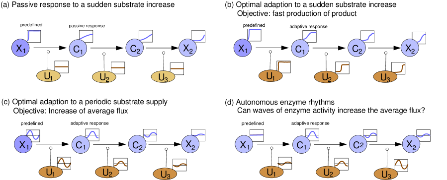
Figure 1: Metabolic dynamics and enzyme adaptation in a linear pathway. Metabolites are shown by circles (dark blue: external substrate with predefined level; light blue: internal metabolites), enzymes are shown by ellipses. Each enzyme produces the substrate for the following enzyme. (a) Constant enzyme levels (yellow). After a sudden increase in substrate level, metabolite levels increase along the chain with different time delays. (b) Optimal temporal enzyme profile (brown). Following a “just-in-time” strategy, enzymes are induced sequentially. This sequential activation can speed up the process (i.e. the time until half of the substrate has been turned into product) at a fixed total enzyme cost [14, 15]. (c) “Just-in-phase” enzyme rhythm as an optimal adaptation to a periodic substrate supply. Substrate oscillations alone would lead to metabolite oscillations. Adaptative enzyme rhythms can modify these rhythms, increasing average flux and catalytic rate. (d) A self-promoting enzyme rhythm creates metabolite and flux rhythms even in a constant environment. In the article I discuss how externally promoted or self-promoting rhythms can be beneficial and what determines their optimal phases and amplitudes.

Enzyme rhythms may serve as adaptations to external rhythms or as a way to drive “spontaneous” metabolic cycles. The two cases are closely related. By “pumping”, a metabolic cycle can create favourable biochemical conditions at different times in different parts of the network. If we look at individual pathways, the effect of these self-promoting beneficial changes is not very different from (temporally varying) favourable conditions caused by an external oscillation. Then, the cell can exploit this dynamics oscillations by investing enzyme wherever conditions are favourable, leading to periodic enzyme activity changes, phase-shifted along the pathways. In an autonomous metabolic cycle, each pathway is surrounded by a periodic environment – the rest of the network – to which it needs to adapt. If the pathway is optimally adapted to a surrounding system, we can take the surrounding system’s behaviour as given, no matter if we regard it as optimal or as predefined. Therefore, whether rhythms are promoted by the cell’s environment or whether they emerge in the cell, the incentives for enzyme adaptation are the same on the level of single reactions or pathways. We may also argue: if cells can take advantage of oscillations in their environment, which makes metabolic pathways work more efficiently, they may achieve similar benefits by enforcing similar oscillations inside the cell. Once a metabolic cycle has been established (perhaps at some cost), other processes may become adapted to it, creating benefits in different places that lead, overall, to a net advantage. Following these two arguments, I describe both types of rhythms – promoted and self-promoting rhythms – by one theory. To see whether rhythms can improve metabolic performance, I study dynamic metabolic models and search for periodic enzyme profiles that optimise the performance of some biological function.

How can optimal enzyme rhythms be predicted from mathematical models? Here we consider an optimal control problem based on metabolic efficiency. We describe the system under study (a metabolic pathway or network) by a kinetic model and ask how enzyme oscillations (as opposed to static enzyme levels) can improve the performance of the system, e.g. the average flux per average enzyme amount. Mathematically, metabolite concentrations and rates are described by a kinetic model an enzyme profiles are optimised. This approach has been applied to static enzyme levels [16], static enzyme adaptation [17] and temporal enzyme profiles [14, 15]. For example, imagine a metabolic pathway in which the substrate level switches from zero to some constant positive value. How should the enzymes be activated in time? If all enzyme activities were constant, the metabolite concentrations would slowly increase one after the other (Figure 1 (a)). By choosing time-dependent enzyme profiles, the chemical conversion can be accelerated at a constant enzyme investment. Optimisations of enzyme profiles [14] or enzyme regulation mechanisms [15] predicted a sequential induction of enzymes (Figure 1 (b)), a behaviour observed in amino acid biosynthesis pathways [15]. In [14], a sequential induction of enzymes was predicted: each enzyme became active only when enough of its substrate had accumulated. The resulting sequential expression was dubbed “just-in-time production” because enzymes are expressed only when needed. Here I ask the same question for periodic states. If the concentration of a pathway substrate changes periodically, can synchronous enzyme rhythms increase the average flux and thereby the catalytic rate? Can we expect wave-like activity patterns that “push” or “guide” metabolites along a pathway (Figure 1 (c))? And can autonomous enzyme waves increase metabolic efficiency, even in a static environment (Figure 1 (d))?

Here I propose a theory of optimal enzyme rhythms in kinetic metabolic models, applicable from small pathways to entire metabolic networks. Enzyme rhythms can be understood in two ways: causally, through physical mechanisms, and functionally, through economic demands. To combine these two views, I consider kinetic metabolic models with optimal enzyme profiles. In the models, optimal enzyme activities are not determined by regulation (e.g. transcriptional gene regulation), but by their function, i.e. by benefits they provide. The focus on optimal profiles rather than regulation mechanisms is reflected in my terminology. If an external rhythm provides an incentive for enzyme rhythms, we say that it “promotes” the enzyme rhythm. Likewise, if an enzyme rhythm provide a fitness advantage just by itself, in a static environment, this rhythm is called self-promoting. Whether and how these optimal rhythms can be realised by cells is a separate question and should be discussed separately.

To define optimality problems for enzyme rhythms, I assume a given environment (e.g. static or periodic external substrate levels) and search for periodic enzyme profiles that lead to a maximal fitness. Then, to obtain tractable formulae, I apply a perturbation theory: oscillations are described by small sine-wave oscillations around an enzyme-optimised steady reference state, and all oscillating variables (enzyme activities, metabolite concentrations, and fluxes) are represented by amplitudes and phases (“curve parameters”). To relate the amplitudes and phases of different metabolites, enzyme, and fluxes, periodic response coefficients from Metabolic Control Theory (MCT) are used [18]. With all these approximations, finding optimal enzyme profiles becomes a quadratic optimality problem with linear constraints (see Figure A in appendix). If none of the constraints are hit, the adaptations to perturbations at different frequencies are additive and the adaptations to non-sine-wave perturbations can be obtained by Fourier synthesis. The search for optimal enzyme rhythms resembles a search for optimal static enzyme adaptations, which has been addressed in [17]. Optimal static enzyme adaptations can be computed from metabolic response coefficients and curvatures of the fitness function. Similarly, to compute optimal enzyme rhythms, we replace real-valued static adaptations by complex-valued oscillation amplitudes, and static response coefficients by their complex-valued, periodic counterparts. A new finding is that periodic enzyme variations can improve an already optimal state, even if static enzyme shifts cannot provide an advantage.

In this article I extend the theory of optimal enzyme adaptation from [17] into a theory of optimal enzyme rhythms. The text is structured as follows. I first consider a single reaction and show how a given substrate rhythm can provide an incentive for enzyme rhythms. Then I study optimal enzyme rhythms across an entire network and derive formulae for enzyme amplitudes and phases in externally promoted or self-promoting rhythms. Known formulae for static enzyme adaptation [17] are reobtained as a special case. Finally, I ask how enzyme rhythms should be realised by combining gene expression and posttranslational modifications. As expected, transcriptional regulation is preferably used for slow changes, while posttranslational regulation is preferably used for faster changes. While this article shows simple example models, the theory applies to networks of any size. Mathematical details are given in the appendix and in the supplementary material. More examples are shown at www.metabolic-economics.de/enzyme-rhythms/.

Box 1: Beneficial enzyme oscillations in a single reaction
Figure (a) shows a reaction X $\rightarrow$ Y with an irreversible mass-action rate law $\nu(u,x)=u\,k\,x$ and a given substrate rhythm $x(t)$. The enzyme activity $u(t)$ describes the concentration of active enzyme. We consider the reaction rate $v$ in mM/s, enzyme activity $u$ in mM, substrate level $x$ in mM, rate constant $k$ in mM^-1 s^-1. What is the enzyme rhythm $u(t)$ (with a given average value) that maximises th average flux? We assume sine-wave profiles $\displaystyle x(t)=\bar{x}+\mbox{Re}(\mbox{\rm e}^{i\omega t}\,{\tilde{x}}),\qquad u(t)=\bar{e}+\mbox{Re}(\mbox{\rm e}^{i\omega t}\,{\tilde{e}})$ (1) with mean values $\bar{x}$ and $\bar{e}$ and complex amplitudes ${\tilde{x}}$ and ${\tilde{e}}$. Circular frequency $\omega$, frequency $f$, and period $T$ are related by $\omega=2\,\pi\,f=2\,\pi/T$. By inserting the profiles $x(t)$ and $u(t)$ into the rate law, we obtain the time-dependent reaction rate $\displaystyle v(t)$ $\displaystyle=$ $\displaystyle\underbrace{k\,\bar{e}\,\bar{x}}_{\bar{v}}+\underbrace{k\,\mbox{Re}(\mbox{\rm e}^{i\omega t}\,{\tilde{e}})\bar{x}}_{\langle\cdot\rangle_{t}=0}+\underbrace{k\,\bar{e}\,\mbox{Re}(\mbox{\rm e}^{i\omega t}\,{\tilde{x}})}_{\langle\cdot\rangle_{t}=0}+\underbrace{k\,\mbox{Re}(\mbox{\rm e}^{i\omega t}\,{\tilde{e}})\,\mbox{Re}(\mbox{\rm e}^{i\omega t}\,{\tilde{x}})}_{\frac{k}{2}\mbox{Re}(\mbox{\rm e}^{i2\omega t}\,{\tilde{e}}\,{\tilde{x}})+\frac{k}{2}\mbox{Re}({\tilde{e}}^{*}\,{\tilde{x}})},$ (2) a sum of five terms: a static reference flux $\bar{v}$, two periodic terms caused by linear effects of the periodic parameters, and two synergy terms (see SI LABEL:sec:proofFourTerms). The synergy term $\frac{k}{2}\mbox{Re}(\mbox{\rm e}^{i2\omega t}\,{\tilde{e}}\,{\tilde{x}})$ describes an oscillation of frequency $2\,\omega$, while the synergy term $\Delta\bar{v}=\frac{k}{2}\mbox{Re}({\tilde{e}}^{*}\,{\tilde{x}})$, with a star for the complex conjugate, describes a shift of the average flux [18]. This flux shift is the benefit we are interested in. It is given by $\displaystyle\Delta\bar{v}=\langle\Delta v\rangle_{t}=\frac{k}{2}\,|{\tilde{x}}|\,|{\tilde{e}}|\,\cos(\Delta\varphi)$ (3) and can be positive or negative depending on the phase difference $\Delta\varphi=\varphi({\tilde{x}})-\varphi({\tilde{e}})$ (Figure (b)). Instead of a mass-action rate law, we may consider more general nonlinear rate laws $\nu=u\,k(x)$. We assume small oscillation amplitudes and use the linear approximation $\displaystyle\Delta\bar{v}=\langle\Delta v(t)\rangle_{t}=\frac{E_{\rm x}}{2\bar{e}}\,|{\tilde{x}}|\,|{\tilde{e}}|\,\cos(\Delta\varphi)$ (4) with the unscaled elasticity $E_{\rm x}=\partial\nu/\partial x$ (see SI section LABEL:sec:nonlinear). For fully saturated enzymes (with $E_{\rm x}=0$), the oscillation has no effect on the average flux. As shown in the graphics above (Figure (b)), the average flux $\langle v\rangle_{t}=\bar{v}+\Delta\bar{v}$ depends on the phase shift between substrate and enzyme. If substrate and enzyme vary in phase ($\Delta\varphi=0$), the flux increases by $\frac{E_{\rm x}\,|{\tilde{e}}|\,|{\tilde{x}}|}{2\bar{e}}$. The overall efficiency $\langle v\rangle_{t}/\langle u\rangle_{t}$ – the average rate, divided by the average enzyme level – increases while average enzyme activity and average ratio $\langle v/u\rangle_{t}=k\langle x\rangle_{t}=k\,\bar{x}$ remain unchanged. In contrast, if $x(t)$ and $u(t)$ oscillate with opposite phases, catalytic rate and average flux may decrease.

2 Optimal enzyme profiles

2.1 Periodic enzyme levels can increase the catalytic rate

Let us see how a periodic redistribution of enzyme resources can improve metabolic performance. If a reaction’s substrate level varies periodically, a synchronous periodic variation of enzyme activity (at a constant average enzyme level) can be beneficial. Whenever the substrate level is high, the enzyme acts more efficiently: shifting enzyme investments to these moments will increase the average flux per average enzyme activity: the oscillations can increase average fluxes “for free”! Box 1 shows an example. The fact that oscillations can provide an advantage challenges a basic assumption in metabolic modelling, the assumption that optimal metabolic states need to be steady states.

Here I will call this phenomenon – synergisms due to synchronised substrate and enzyme rhythms – “allosynchrony”. Unlike allosteric regulation, which acts in each moment in time, allosynchrony concerns the overall time profile and describes the effect of synchronous fluctuations on the average metabolic state. Similar to channelling, which increases the local substrate concentration “seen” by the enzyme, allosynchrony increases the substrate concentration “locally in time”, in moments when most enzyme is most abundant. This efficiency increase is achieved by metabolic dynamics, but it also affects cell economy, namely the economical usage of enzymes. A higher metabolic efficiency (average flux per average enzyme activity) leads to a higher economic efficiency (i.e. metabolic benefit per enzyme investment). When enzyme profiles are compared at a given cost (e.g. identical average enzyme levels, and assuming a linear cost function), high cost efficiency implies a high metabolic objective. If a substrate rhythm allows cells to increase their average fluxes at a given enzyme cost, there will be an incentive for such enzyme rhythms – in other words, they will be promoted.

In metabolic pathways or networks, enzyme resources can be reallocated not only in time, but also across reactions. If the periodic metabolite concentrations were known, we could determine optimal enzyme rhythms reaction by reaction, as described above. However, in kinetic models the internal metabolite concentrations are not predefined, but depend on the enzyme levels! Thus, our optimality problem contains various degrees of freedom: all enzyme rhythms must be optimised simultaneously, taking into account their dynamic effects on metabolite concentrations. All this makes the problem much harder. For example, each oscillating enzyme has an adverse effect on its own substrate: whenever an enzyme level is high, the substrate level tends to go down, when the enzyme level is low, the substrate accumulates. Due to this adverse effect, enzyme rhythms tend to decrease an enzyme’s average efficiency [20]! To obtain a beneficial overall rhythm, these adverse effects need to be overcompensated by beneficial effects, e.g. by creating phases in which certain enzymes have a higher thermodynamic efficiency [10]. Moreover, enzymes may also be coupled through costs. For example, if there is a fixed overall enzyme budget, but investments can be reallocated between enzymes in every moment, the increasing one enzyme level implies decreasing another one Mathematically, rhythms in a networks resemble rhythms in a single reaction, but with some additional complications. First, only some of the metabolite profiles are predefined, while all others are determined by the system dynamics and dependent on enzyme profiles. Second, perturbations propagate through the networks dynamically, and in finding optimal enzyme amplitudes and phase patterns, we need to account for this. Third, all enzyme profiles are optimised simultaneously and must be adapted to the effects of other enzyme rhythms, which are optimally adapted as well. The result is a self-consistent, optimal metabolic state.

To model how enzyme rhythms shape metabolic states and are shaped by them at the same time, we need to first consider metabolic dynamics and understand how enzyme levels act on metabolite concentrations and fluxes. Then we turn its logic around, interpreting the possible effects of an enzyme change as an incentive, or teleological cause, for this change. When a reaction rate is perturbed, the perturbation propagates through the network, reaching different parts of the network with different delays: the details of this forward propagation – where perturbations arrive, with what delays, and how they are damped – are themselves reflected in the necessary or optimal enzyme profiles. In the following sections, we develop a theory of optimal enzyme rhythms in three steps: (i) we define an optimality problem for periodic metabolic states; (ii) we compute synergy effects between oscillating model parameters (external parameters and enzyme levels), which depend on oscillation amplitudes and phase shifts; (iii) and we determine an optimal network-wide enzyme rhythm that maximises the sum of all synergy effects.

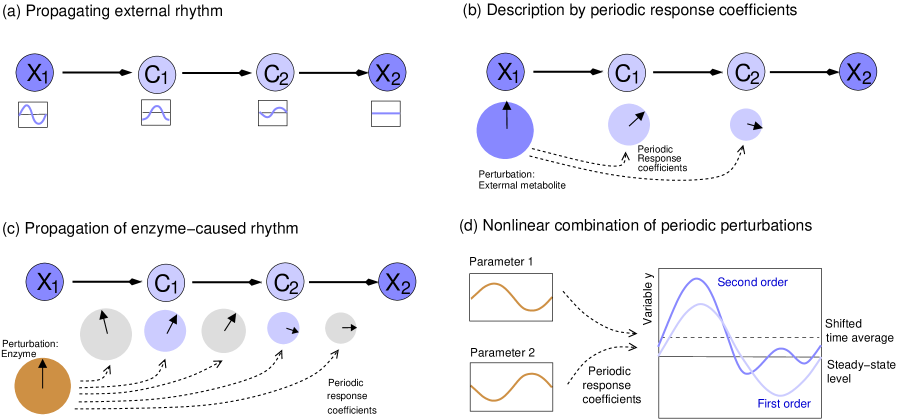
Figure 2: Forced oscillations in a metabolic pathway (schematic example). (a) Metabolic pathway with external substrate rhythm. The periodic substrate level $x_{1}(t)$ (blue curve) causes metabolite and flux variations that propagate down the pathway as damped waves. (b) Forced oscillations in a model with linearised rate laws $\Delta{\bf v}(t)\approx{\bf E}_{\rm u}\Delta{\bf e}(t)+{\bf E}_{\rm c}\Delta{\bf c}(t)+{\bf E}_{\rm x}\Delta{\bf x}(t)$. Amplitudes and phases are described by complex amplitudes (pointer lengths and angles). The amplitude of metabolite $i$ is obtained by multiplying the amplitude of the perturbed parameter (index $m$) with the spectral response coefficient $\tilde{R}^{c_{i}}_{p_{m}}(\omega)$ between parameter $p_{m}$ and concentration $c_{i}$. (c) Metabolite and flux oscillations enforced by enzyme rhythms. (d) Synergistic parameter rhythms. A pair of periodic parameters (with circular frequency $\omega$) leads to oscillations in a state variable $z$; in a second-order approximation, the forced oscillation consists of an average shift (second-order effect), a sine-wave oscillation of frequency $\omega$ (first-order effect), and a second harmonic (frequency $2\omega$, second-order effect).

2.2 Dynamics of enzyme rhythms in pathways and networks

To predict beneficial enzyme rhythms, we first need to model the metabolic dynamics, i.e. the effect of enzyme rhythms on metabolite levels and fluxes. To do so, we consider a kinetic model with internal concentrations $c_{i}$ and reaction rates $v_{l}$ as state variables. The rate laws depend on metabolite concentrations $c_{i}$, external metabolite concentrations, $x_{j}$, and enzyme activities $e_{l}$. If enzyme activities oscillate, they evoke oscillations in internal metabolite concentrations and fluxes. The amplitudes and phases depend on network structure, rate laws, enzyme amplitudes, and oscillation frequency. If oscillations are small, amplitudes and phases can be predicted from spectral response coefficients [21, 18] (see Figure 2). In the calculation, we start from a steady reference state with constant external parameters and optimal enzyme activities (which must be a stable steady state). Then we consider sine-wave oscillations of external parameters $x_{j}(t)$ and enzyme activities $e_{l}(t)$ around this state (with circular frequency $\omega$ and complex amplitudes ${\tilde{x}}_{j}$ and ${\tilde{e}}_{l}$). In addition, we may apply shifts $\Delta\bar{x}_{j}$ and $\Delta\bar{e}_{l}$ of the average values. Then we apply perturbation theory: the state variable profiles are approximated by the leading terms of a Taylor expansion. In a linearised model, sine-wave perturbations lead to sine-wave metabolite and flux oscillations of the same frequency, and the amplitude profiles $\tilde{{\bf c}}$ and ${\tilde{\bf v}}$ of the state variables depend linearly on the amplitude profiles ${\tilde{\bf x}}$ and ${\tilde{\bf e}}$ of the perturbed parameters. We can write the dynamics as $\tilde{{\bf c}}=\tilde{\bf R}^{\rm S}_{\rm\tilde{x}}\,{\tilde{\bf x}}+\tilde{\bf R}^{\rm S}_{\rm\tilde{u}}\,{\tilde{\bf e}}$, with expansion coefficients given by the spectral response coefficients (in matrices ${\bf R}^{\rm S}_{\rm\tilde{x}}$ and $\tilde{\bf R}^{\rm S}_{\rm\tilde{u}}$), and an analogous formula holds for flux amplitudes ${\tilde{\bf v}}$ [18]. Similarly, average parameter shifts $\Delta{\bf x}$ and $\Delta{\bf e}$ lead to average shifts $\Delta\bar{{\bf c}}=R^{\rm S}_{\rm x}\,\Delta{\bf x}+R^{\rm S}_{\rm u}\,\Delta{\bf e}$ with static response coefficients as prefactors. Generally, linearised metabolic models act as low-pass filters: at low frequencies, there is a quasi-static response, while at high frequencies perturbations are strongly damped. At intermediate frequencies, dynamic resonance may occur [18]. To handle combined perturbations, involving multiple perturbations and frequencies, we can split them into sums or integrals of basic perturbations (with single perturbations and frequencies), and sum over the dynamic responses. This linear superposition works in the first-order approximation only. At larger perturbation amplitudes, the approximation becomes unreliable and we need to include higher-order effects: in a second-order approximation, the synergistic interactions between enzymes lead to second harmonics at frequency $2\,\omega$ and to shifts in the average concentrations and fluxes (see appendix A and SI LABEL:sec:periodicdynamics).

2.3 Optimal rhythms in metabolic pathways and networks

If we know how to simulate enzyme rhythms and their effects on metabolic fluxes, we can also turn this around and ask: what enzyme profiles are needed to obtain a certain desired system output? For example, given an external metabolite rhythm ${\tilde{\bf x}}$, which enzyme profiles could realise a desired flux oscillation at a minimal cost? Such inverse problems can be hard, but our small-amplitude approximation makes them tractable (see SI LABEL:sec:achievepredefineddynamic). To formulate cost-benefit problems for metabolic networks (see Figure 10), we combine the internal metabolite concentrations $c_{i}$ and fluxes $v_{l}$ into a state vector ${\bf z}$ and define a metabolic objective function $y({\bf z})$. The vector ${\bf z}$ may also include other state variables such as pH values, membrane potentials, or organelle volumes. In our optimality problem, we consider two types of parameters: external parameters $x_{j}$ imposed by the environment (here usually external metabolite concentrations), and control variables $e_{l}$ to be optimised (here usually enzyme activities $e_{l}$). As a fitness function, we consider the difference ${\mathcal{F}}({\bf e},{\bf x})=q({\bf e},{\bf x})-h({\bf e})$ of a metabolic objective $q({\bf e}.{\bf x})=y({\bf z}({\bf e},{\bf x}))$ and an enzyme cost $h({\bf e})$ [22, 23]. Typically, the metabolic objective $y({\bf c},{\bf v})$ requires high production fluxes and low metabolite concentrations, while the cost $h$ increases with the enzyme activities $e_{l}$.

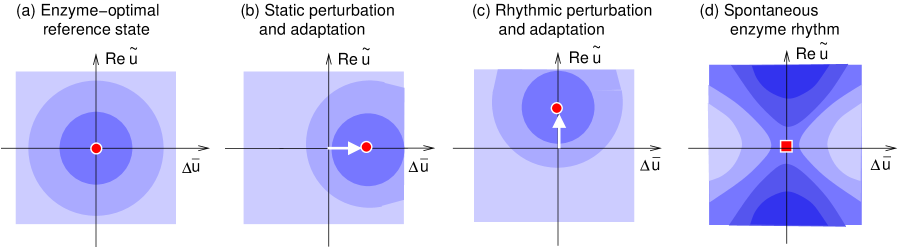
Figure 3: Prediction of optimal enzyme profiles. A periodic enzyme profile, described by a static shift $\Delta\bar{e}$ and complex-valued amplitude ${\tilde{e}}$ for a single enzyme, influences the behaviour of a metabolic system (compare Figures A (a) and 10). The resulting fitness of the metabolic system can be described by a fitness function $F(\Delta\bar{e},{\tilde{e}})$ in the space of enzyme profiles. The different panels show fitness landscapes under different external metabolite perturbations $\Delta\bar{x}$ or ${\tilde{x}}$. A red dot marks the optimal state. (a) Unperturbed fitness landscape ($\Delta\bar{x}={\tilde{x}}=0$, leading to $\Delta\bar{e}={\tilde{e}}=0$; fitness contours shown in blue; dark blue represents high fitness). The fitness maximum lies in the reference state. Negative fitness curvatures for $\Delta\bar{e}$ and ${\tilde{e}}$, described by fitness synergies $F_{\rm uu}$ and $F_{\rm\tilde{u}\tilde{u}}(\omega)$ in this point, show that any change $\Delta u$ or ${\tilde{e}}$ would decrease the fitness. (b) An external parameter shift $\Delta\bar{x}$ changes the landscape, displaces the optimum point, and promotes a static shift $\Delta\bar{e}^{\rm opt}$ of the optimal enzyme level. (c) An external rhythm with amplitude ${\tilde{x}}$ displaces the optimum and promotes an enzyme rhythm with amplitude ${\tilde{e}}^{\rm opt}$. (d) The reference state is a saddle point of the fitness landscape (red square), fitness-unstable against enzyme rhythms. Any static enzyme change $\Delta u$ would decrease the fitness, but some oscillations (${\tilde{e}}\neq 0$) increase the fitness even in the absence of external oscillations. These beneficial oscillations are called “self-promoting”.

To study optimal enzyme rhythms, we start from a steady reference state with given external concentrations $x_{j}^{\rm ref}$ and static enzyme levels $e_{l}^{\rm ref}$ that are already optimised. As an optimality condition, ${\mathcal{F}}({\bf e},{\bf x})$ must have negative curvatures with respect to ${\bf e}$ (except for those enzymes that are not used in this optimal state). Based on this state we study the adaptation of the enzyme profile to external perturbations. To define our optimality problem, we use a functional that assigns fitness values to metabolic time courses. We consider two possibilities, the state-average fitness ${\mathcal{F}}=y(\langle{\bf z}\rangle_{t})-h(\langle{\bf e}\rangle_{t})$ and the fitness-average fitness ${\mathcal{F}}=\langle y({\bf z})-h({\bf e})\rangle_{t}$. Both of them are based on time averages: in one case the static fitness function ${\mathcal{F}}$ is applied to the average metabolic state, in the other one the fitness is evaluated in every moment and then averaged over time, which means that variations around the average value can have a fitness effect. Using our fitness functional, we can study the fitness changes caused by perturbations and adaptations. If a static parameter change $\Delta{\bf x}$ is applied to our reference state, the optimal enzyme adaptation $\Delta{\bf e}$ follows from the second-order metabolic response coefficients [17]. With periodic external perturbations, the calculation works similarly, but using periodic response coefficients [18] (see SI LABEL:sec:periodicdynamics). Let us see how this works. We start from our optimal reference state, apply periodic external profiles ${\bf x}(t)={\bf x}^{\rm ref}+\Delta{\bf x}+\mbox{Re}(\mbox{\rm e}^{i\,\omega\,t}\,{\tilde{\bf x}})$ and enzyme profiles ${\bf e}(t)={\bf e}^{\rm ref}+\Delta{\bf e}+\mbox{Re}(\mbox{\rm e}^{i\,\omega\,t}\,{\tilde{\bf e}})$, and evaluate the resulting periodic state (Figure 3 (b)). The fitness can be written as a function ${\mathcal{F}}(\Delta{\bf e},\Delta{\bf x},{\tilde{\bf e}},{\tilde{\bf x}})$ of the shifts $\Delta{\bf e}$ and $\Delta{\bf x}$ and of the complex amplitude profiles ${\tilde{\bf e}}$ and ${\tilde{\bf x}}$ (see Figure 3). Near the reference state, a second-order approximation yields

$$\Delta{\mathcal{F}}(\Delta{\bf e},{\tilde{\bf e}},\omega)\approx\underbrace{\left[\Delta{\bf x}^{\top}\,{\bf F}_{\rm xe}\Delta{\bf e}+\frac{1}{2}\Delta{\bf e}^{\top}\,{\bf F}_{\rm ee}\Delta{\bf e}\right]}_{\mbox{static}}+\underbrace{\left[\mbox{Re}({\tilde{\bf x}}^{{\dagger}}\,{\bf F}_{\rm\tilde{x}\tilde{e}}(\omega)\,{\tilde{\bf e}})+\frac{1}{2}{\tilde{\bf e}}^{{\dagger}}\,{\bf F}_{\rm\tilde{e}\tilde{e}}(\omega)\,{\tilde{\bf e}}\right]}_{\mbox{periodic}}.$$ (5)

The shape of the the fitness landscape near the reference state depends on the local curvatures of ${\mathcal{F}}$ with respect to $\Delta{\bf e}$, $\Delta{\bf x}$, ${\tilde{\bf e}}$, and ${\tilde{\bf x}}$, contained in the fitness synergy matrices (${\bf F}_{\rm ee}$ and ${\bf F}_{\rm ex}$ for static variations, ${\bf F}_{\rm\tilde{e}\tilde{e}}$ and ${\bf F}_{\rm\tilde{e}\tilde{x}}$ for periodic variations) as components. The synergies depend on the kinetic model, on cost and benefit functions, and on the type of fitness functional used (state-average or fitness-average fitness). If the reference state is known, the curvature matrices can be easily computed with formulae from MCT (see appendix B). What can we learn from the fitness expansion in Eq. (5)? The first bracket term describes the effect of static perturbations (and enzyme adaptation), while the second bracket describes the effect of parameter rhythms (and adaptative enzyme rhythms) at frequency $\omega$. In the formulae, irrelevant terms have been omitted: terms that depend only on $\Delta{\bf x}$ and ${\tilde{\bf x}}$ do not matter for the choice of the enzyme profiles; terms linear in $\Delta{\bf e}$ vanish because of the optimality condition ${\bf f}_{\rm u}=0$ in the reference state; and terms linear in ${\tilde{\bf e}}$ do not lead to any shifts on time average. The expansion formula Eq. (5) holds for sine-wave perturbations of frequency $\omega$. Due to the second-order approximation (and assuming a time-independent fitness function), there are no synergies between perturbations of different frequencies, or between static and periodic perturbations. To compute the effects of mixed perturbations with multiple parameters and multiple frequencies, we can sum or integrate over the adaptive responses at different frequencies.

To summarise, the fitness effect of an enzyme profile can be computed via the synergy matrices ${\bf F}_{\rm ee}$ and ${\bf F}_{\rm ex}$ (for static adaptation) or ${\bf F}_{\rm\tilde{e}\tilde{e}}$ and ${\bf F}_{\rm\tilde{e}\tilde{x}}$ (for adaptive rhythms). The matrix elements represent three sorts of synergies: synergies between external parameters and enzymes (elements of ${\bf F}_{\rm ex}$ and ${\bf F}_{\rm\tilde{e}\tilde{x}}$), synergies between different enzymes (off-diagonal elements of ${\bf F}_{\rm ee}$ and ${\bf F}_{\rm\tilde{e}\tilde{e}}$), and enzyme self-synergies (diagonal elements of ${\bf F}_{\rm ee}$ and ${\bf F}_{\rm\tilde{e}\tilde{e}}$). All three effects together determine the total fitness effect of an enzyme profile: if it is positive, the enzyme rhythm provides an advantage over the unperturbed steady state. Enzyme self-synergies are usually negative because of dynamic self-inhibition or because of the effect of diminishing returns (due to fitness-average fitness functionals with non-linear cost functions). To make enzyme rhythms beneficial this negative effect must be overcompensated by beneficial synergy effects between external parameters and enzymes or between different enzymes.

2.4 Promoted and self-promoting enzyme rhythms

If an external parameter shift $\Delta\bar{x}$ or an external rhythm ${\tilde{x}}$ is applied to our reference state, how should the (static or periodic) enzyme profile be optimally adapted? The expansion formula (5) helps us answer this question. To compute the profile, we consider the fitness landscape $F(\Delta{\bf e},{\tilde{\bf e}})$, approximate it by Eq. (5), consider an external perturbation ${\bf x}(t)$, and determine the optimal curve parameters (in vectors $\Delta{\bf e}$ and ${\tilde{\bf e}}$) that

$$\mbox{Maximise}\quad\Delta{\mathcal{F}}(\Delta{\bf e},{\tilde{\bf e}},\omega)$$ (6)

under the constraint $\Delta{\bf e}\geq-\bar{\bf e}$. Without external perturbation, the system should stay in the reference state (with $\Delta{\bf e}={\tilde{\bf e}}=0$) because this state is a local fitness optimum. With a static perturbation $\Delta{\bf x}$, the fitness landscape changes and the optimum moves. If the new optimum $\bar{\bf e}$ respects all constraints (e.g. if all enzyme levels remain positive), the displacement $\Delta{\bf e}^{\rm opt}$ yields the optimal enzyme adaptations (Figure 3 (b)). Optimal adaptations to periodic perturbations are computed similarly: an external rhythm with amplitude profile ${\tilde{\bf x}}$ displaces the optimum by ${\tilde{\bf e}}^{\rm opt}$ (in the space of amplitude profiles ${\tilde{\bf e}}$), the vector of amplitudes and phases of the optimal enzyme profile. In both cases, the optimal enzyme profile follows from maximising Eq. (5) with the perturbation $\Delta{\bf x}$ or ${\tilde{\bf x}}$. If there are no no further active constraints, each of the bracket terms (for static and periodic shifts) can be optimised separately. A static perturbation $\Delta{\bf x}$ promotes a static adaptation

$$\Delta{\bf e}^{\rm opt} \approx -{\bf F}_{\rm ee}^{-1}\,{\bf F}_{\rm ex}\,\Delta{\bf x}$$ (7)

while a periodic perturbation profile ${\tilde{\bf x}}$ promotes a periodic adaptation with amplitude profile

$${\tilde{\bf e}}^{\rm opt} \approx -{\bf F}_{\rm\tilde{e}\tilde{e}}^{-1}\,{\bf F}_{\rm\tilde{e}\tilde{x}}\,{\tilde{\bf x}}.$$ (8)

If a mixed perturbation is applied (a sum of static perturbations and periodic perturbations with multiple frequencies), the optimal adapatation is given by the sum of the single optimal adaptations (again, under the conditions mentioned above that allow for linear superposition).

(a) Forced oscillations caused by substrate rhythm		(b) Adaptive enzyme rhythm
External substrate rhythm		Enzyme rhythm
Responsive metabolite rhythm		Metabolite rhythm
Responsive flux rhythm		Flux rhythm

Figure 4: Enzyme rhythm in a metabolic pathway. (a) Forced metabolic oscillations at constant enzyme levels. Top: pathway structure (metabolites shown as circles, X1 and X2 are external metabolites). Fluxes are shown as arrows. Centre: sine-wave oscillations of the external substrate (frequency $f=0.25$ s^-1) cause metabolite oscillations that propagate as damped waves. Amplitudes and phase angles shown by arrows. Bottom: oscillating fluxes caused by the substrate rhythm. (b) Dynamics with optimally adapted sine-wave enzyme rhythm. Top: the first enzyme is almost in phase with the substrate, while the others show larger phase shifts. The resulting metabolite and flux rhythms are shown in the centre and bottom panels.

We saw how enzyme rhythms can be promoted by external rhythms. How can we describe self-promoting rhythms, that is, enzyme rhythms that provide benefits in static environments? Again, we consider a reference state that cannot be improved, at least not by static enzyme changes. However, there may still be enzyme rhythms that lead to improvements even in the absence of external rhythms, there is an incentive for such rhythms. As mentioned above, I call such rhythms “self-promoting”. To increase fitness by enzyme rhythms alone (positive $\Delta F={\tilde{\bf e}}^{\dagger}\,{\bf F}_{\rm\tilde{e}\tilde{e}}\,{\tilde{\bf e}}$), the matrix ${\bf F}_{\rm\tilde{e}\tilde{e}}$ must have a positive eigenvalue (see Figure 3 (d)). To test this, we compute the maximal eigenvalue of ${\bf F}_{\rm\tilde{e}\tilde{e}}(\omega)$, called principal fitness synergy $\sigma(\omega)$. If this value is positive, the corresponding eigenvector describes a self-promoting enzyme rhythm, the most beneficial rhythm at a given amplitude $||{\tilde{\bf e}}||\leq{\tilde{\bf e}}^{\rm max}$. In contrast, if $\sigma(\omega)$ is negative for all frequencies $\omega$, our system is stable against self-promoting enzyme rhythms.

External substrate rhythm

Principal synergy

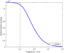
Enzyme rhythm

Metabolite rhythm

Flux rhythm

Figure 5: Self-promoting enzyme rhythm in a linear pathway. Starting from the model in Figure 4, we now assume that metabolites can disappear by dilution, by non-enzymatic degradation, or by passive diffusion through cell membranes. Enzyme rhythms can reduce this loss and increase the production flux, even in the absence of external rhythms. We can see this from the positive principal synergy at low frequencies. Like in Figure 4, we assume that enzyme levels can oscillate without any extra cost.

Self-promoting rhythms may involve the entire metabolic network like the metabolic cycle in yeast. However, to see the reasons for self-promoting oscillations more generally, let us consider a simple examples. In the pathway in Figure 4, a given substrate level and optimally adapted enzyme activities define a static reference state. A quasi-static substrate increase would promote, i.e. favour, an increase in enzyme activities. What behaviour will periodic substrate rhythms promote? At constant enzyme activities, a substrate rhythm would lead to damped concentration and flux waves along the pathway (Figure 4 (a)). But if a wave-like enzyme rhythm is added, orchestrated with the substrate rhythm, the average flux can be increased by allosynchrony. In other words: the substrate oscillation promotes a wave-like enzyme rhythm (Figure 4 (b)). Can an enzyme rhythm alone, without substrate rhythm, be beneficial? In the example, the principal synergy is negative at all frequencies, so there is no incentive for spontaneous enzyme waves. However, this changes if the intermediate metabolites are non-enzymatically degraded. In a model with uncontrollable degradation, spontaneous enzyme rhythms have the potential to increase the average flux at constant external substrate level and are therefore beneficial. (Figure 5). As a variant of the model, we consider a loop-shaped pathway with input and output compounds (Figure 6). Also here, self-promoting enzyme waves can be beneficial: the principal synergy (Figure 6 (b)) has a positive maximum at a finite frequency, caused by a dynamic resonance of the metabolic system, while slower or faster self-promoting oscillations lead to a lower benefit. Regulation systems that generate enzyme rhythms at the optimal frequency will provide a selection advantage. self-promoting oscillations can be seen as an example of spontaneous pattern formation, that is, a pattern formation in time that is not based on dynamics alone, but on incentives and optimal choices (for details, see www.metabolic-economics.de/enzyme-rhythms/).

(a) Network structure	(b) Principal fitness synergy	(c) Enzyme and metabolite rhythm

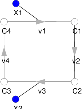
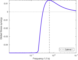
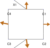
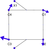
Figure 6: Self-promoting rhythm in a cyclic pathway. (a) Network structure and reference state. A circle flux is driven by an inflow from metabolite X1 and an outflow to metabolite X2. (b) Principal synergy (i.e. maximal fitness curvature) as a function of frequency. The local maximum with a positive value shows an incentive for self-promoting oscillations. (c) Enzyme and metabolite rhythm. The optimal self-promoting enzyme profiles (brown arrows) are phase-shifted along the pathway. Blue arrows show the metabolite rhythm.

2.5 Enzyme rhythms that combine transcriptional and posttranslational regulation

We saw how optimal enzyme rhythms can be computed from synergies given in the matrices ${\bf F}_{\rm\tilde{e}\tilde{x}}$ and ${\bf F}_{\rm\tilde{e}\tilde{e}}$. However, so far we ignored all possible side constraints. These constraints may prevent, for example, that enzyme amplitudes exceed the enzyme’s average value (which would lead to negative values), a problem that may occur if an enzyme is inactive in the reference state and starts oscillating. For example, storage reactions are useless in a strictly static environment: a steady conversion of glucose into glycogen and back would be futile and the reactions should be inactive. However, in a periodic environment, storage and release of glycogen may buffer the fluctuation inside the cell and provide a relatively constant glucose supply, which can be beneficial. Finally, amplitude constraints are also important when desired amplitudes cannot be realised by gene expression at higher frequencies (see SI LABEL:sec:geneexpression). What are the relevant constraints for a profile ${\bf e}(t)=\bar{\bf e}+\Delta\bar{\bf e}+\mbox{Re}(\mbox{\rm e}^{i\,\omega\,t}\,{\tilde{\bf e}})$? Bounds on the amplitudes ${\tilde{\bf e}}$, and constraints between $\bar{\bf e}$ and ${\tilde{\bf e}}$, are obtained as follows. First, to prevent negative enzyme activities, the shifts $\Delta\bar{e}_{l}$ must not go below $-\bar{e}_{l}$ and the amplitude $|{\tilde{e}}_{l}|$ must not exceed the average level $\bar{e}_{l}+\Delta\bar{e}_{l}$. This means that the average level of any oscillating enzyme must be positive. Moreover, if enzyme rhythms are caused by rhythmic mRNA profiles, the enzyme amplitudes at high frequencies become very small and, conversely, there is a bound on the possible enzyme amplitudes (see appendix C and SI LABEL:sec:geneexpression). If we impose such constraints, the solutions $\bar{e}_{l}$ and ${\tilde{e}}_{l}$ from Eqs (7) and (8) may not be valid any longer. Instead, we obtain the optimality problem

$$\mbox{Maximise}\;\;\Delta F(\Delta{\bf e},{\tilde{\bf e}})\quad\mbox{subject to}\quad|{\tilde{\bf e}}|\leq{\tilde{\bf p}}^{\rm max}(\bar{\bf e},\omega)$$ (9)

with the bound $\Delta{\bf e}\geq-\bar{\bf e}$, where $\bar{\bf e}={\bf e}^{\rm ref}+\Delta{\bf e}$. The vector $|{\tilde{\bf e}}|$ contains the absolute values from ${\tilde{\bf e}}$ and ${\tilde{\bf p}}^{\rm max}(\bar{\bf e},\omega)$ describes some frequency-dependent, real-valued amplitude bounds as described above. If a solution $(\Delta{\bf e},{\tilde{\bf e}})$ satisfies all constraints, the constraints can be ignored and we can use the simple formula Eq. (6). This typically holds for adaptive rhythms with small perturbation amplitudes ${\tilde{\bf x}}$, and assuming that all enzymes were active in the reference state. In all other cases, i.e if constraints are active, they affect the solution; if an enzyme hits a constraint, there will be secondary effects on other enzymes and eventually on the entire optimal state (see SI LABEL:sec:RhythmConstraintsLagrange).

(a) Amplitude constraints

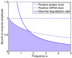
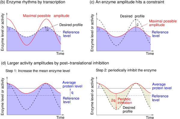
Figure 7: Bounds on enzyme amplitudes create an incentive for posttranslational regulation. (a) Bounds on protein amplitudes (with average concentration $\bar{p}$ and protein degradation constant $\kappa=1$). The blue region shows possible protein amplitudes $\tilde{p}_{l}^{\rm max}(\omega)/\bar{p}_{l}$ at different frequencies. (b) In this case, an enzyme activity profile $u(t)$ respecting the amplitude constraints can be realised by periodic expression. (c) If the desired amplitude is larger, the profile cannot be realised by periodic gene expression alone, and posttranslational regulation needs to be added to achieve the desired amplitude. (d) To increase the activity amplitude while keeping the average activity unchanged, a cell may increase the average enzyme concentration (left) and periodically inhibit the enzyme by posttranslational modification (right). The inhibition amplitude and the increase in average enzyme level, needed for compensation, are both given by $q=|{\tilde{e}}|-{\tilde{p}}^{\rm max}$, the difference between desired activity amplitude and allowed protein amplitude. The extra cost for the higher protein level is proportional to the inhibition amplitude and can be regarded as a cost of the periodic inhibition.

Until now, we assumed that changes in enzyme activities are caused by changing enzyme amounts that is, by changes in gene expression. However, at high frequencies gene expression changes alone will not suffice to realise large enzyme amplitudes, because the dynamics of transcription and translation will damp any changes. To generate larger enzyme activity amplitudes, a cell could periodically inhibit its enzymes by posttranslation modification, such as phosphorylation or acetylation. What is the cost of such posttranslational regulation mechanisms? And how should the two mechanisms be combined? With expression changes alone, and with a linear enzyme cost function (or a state-average fitness functional), the cost of a periodic enzyme profile depends directly on the average enzyme levels, and the periodic fluctuations around it are cost-neutral. Posttranslational activity changes, in contrast, allow us to bypass the amplitude constraint, but now the enzyme rhythms are, effectively, costly. We can see this as follows: if a desired enzyme amplitude $|{\tilde{e}}|$ exceeds the maximal possible protein amplitude ${\tilde{p}}^{\rm max}$, the difference $|{\tilde{e}}|-{\tilde{p}}^{\rm max}$ can only be realised posttranslationally, i.e. by increasing the average enzyme level and applying rhythmic posttranslational inhibition. In this way, the desired amplitude is realised while keeping the average activity unchanged (see Figure 7). The extra cost is proportional to the amplitude difference. To account for this cost in a numerical optimisation, we can introduce an auxiliary variable $q$ for each enzyme, describing the difference between desired enzyme activity amplitude and maximal protein amplitude: this amplitude difference is the amount by which the average enzyme concentration must be increased (see appendix E). The resulting model allows for fast high-amplitude oscillations, but since enzyme modification rhythms are costly, they need to be beneficial! In Figure 8, we consider again the linear pathway from Figure 4 with optimal enzyme rhythms realised by expression changes and posttranslational regulation. As expected, slow enzyme rhythms (on the time scale of hours) are realised by expression changes, while fast oscillations are mostly realised posttranslationally. Notably, expression and posttranslational modification rhythms must be in phase (i.e. posttranslational inhibition should be strongest when enzymes expression is low) because otherwise enzyme resources are wasted.

(a) Enzyme amplitudes (assuming that fast activity changes are possible)

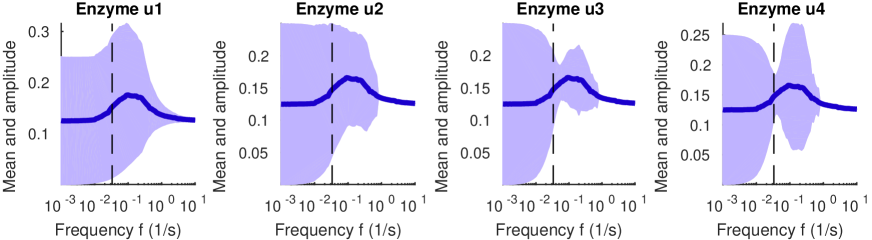
(b) Enzyme amplitudes (combination of slow gene expression changes and fast covalant modification)

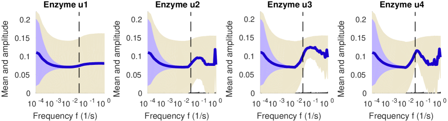
Figure 8: Optimal enzyme rhythms, realised by gene expression and posttranslational regulation. (a) Enzyme amplitudes in a linear pathway (see Figure 4) as a function of frequency $f=\omega/(2\,\pi)$. In the upper panels, we make the (unrealistic) assumption that any enzyme rhythms can be realised transcriptionally, even at high frequencies. Each plot shows to one of the enzymes. Curves show the average enzyme activities; blue bands indicate amplitudes (phase angles not shown). The dashed line denotes the oscillation frequency $f=0.25\,\mbox{s}^{-1}$ from Figure 4. (b) In the lower panels we assume that gene expression can only generate limited amplitudes and that higher amplitudes need to be realised by additional protein modification. Blue areas show expression amplitudes, grey areas show amplitudes by posttranslational modifications. For optimality reasons, both oscillations must be in phase (see Figure 7). Their total enzyme activity amplitude, is shown by the outer envelope. Colours correspond to amplitudes in Figure 7. Even a simple model like this shows complicated regulation profiles. At low-frequency perturbations, the enzymes oscillate in phase with the external perturbation (phases not shown); at high frequencies, enzymes 3 and 4 oscillate in opposite phase. At intermediate frequencies ($\approx$ 0.5  s^-1 for enzyme 3, or $\approx$ 0.1  s^-1 for enzyme 4), the phases of these two enzymes flip (not shown) and their amplitudes become very small.

To summarise, constraints on enzyme amplitudes leads to more realistic predictions of enzyme rhythms and to new types of predicted behaviour. Constraints are especially important if enzymes are not (or weakly) expressed in the reference state or if there is an incentive for fast oscillations (that is, oscillating much faster than the typical time scale of protein dynamics, which for growing cells is typically given by the cell-cycle period). In the first case, an increasing enzyme amplitude may require an increase in the average value. For example, if an enzyme in the reference state is inactive (e.g. the enzymes catalysing glycogen storage and consumption), then in order to oscillate, it must increase its average level from zero to a value as big as the enzyme amplitude. This increase is costly (see appendix E), so it needs to be justified by a benefit. In the second case, protein amplitudes may be limited due to the slow dynamics of protein concentrations. At higher frequencies, gene expression changes will lead to very small amplitudes, and posttranslational modification (e.g. phosphorylation) have to be used instead.

3 Design principles for enzyme rhythms

3.1 Optimal rhythmic enzyme profiles reflect pairwise synergies

Box 2: Dynamics and economics of enzyme rhythms
Metabolic dynamics
Metabolic models with constant enzyme levels can describe the mechanistic effects of external perturbations (e.g. external metabolite concentrations). If we start from a stable steady state and assume a (static or periodic) parameter perturbation, the system’s response – the change of steady-state concentrations and fluxes – can be approximated with the help of metabolic control or response coefficients. Metabolic steady states can be dynamically unstable: if a parameter change destabilises a stable state, this is called a dynamical bifurcation. Left: A metabolic pathway described by reactions, metabolites, and enzymes. Centre: In a kinetic model, metabolite concentrations determine reaction rates, and reaction rates lead to changes of metabolite levels. The causal connections arise from elasticities $E_{li}$ (from compounds to reactions) and stoichiometric coefficients $n_{il}$ (from reactions to compounds), ginving rise to the Jacobian matrix $\mathbf{M}={\bf N}\,\mathbf{E}$ for metabolite concentrations. Right: Metabolic response coefficients translate local perturbations (of enzyme activities and external substance levels) into global responses of all state variables (metabolite concentrations or fluxes). Enzyme economics
On top of metabolic dynamics, we may consider optimal enzyme adaptations, described by optimality problems for enzyme levels. Starting from a (dynamically and economically stable) state, the optimal adaptation to small perturbations can be described by adaptation coefficients (assuming a linear approximation). An optimal steady state may be economically unstable against enzyme oscillations, and transitions from economically stable to an economically unstable states can be described as economic bifurcations. Left: Enzyme profiles lead to metabolic objective (via the state variables) and enzyme cost. Centre: Fitness effects of rhythmic perturbations. In a second-order approximation, fitness depends on pairwise synergies between oscillating parameters (blue arrows), where arrow heads denote beneficial phase relations (pointing towards the element that should peak later). Negative self-synergies are shown by red arcs. Right: Under the optimality principle, an external rhythm promotes a network-wide enzyme rhythm (i.e. it provides an incentive for a rhythm with specific amplitudes and phases). In the example, the second enzyme will show a smaller amplitude and a larger phase shift. The adaptive enzyme profile is shaped by metabolic network structure, metabolic objective function, and the specific perturbation applied.

(a) Network and fluxes	(b) Synergies on network	(c) Synergy phase plot

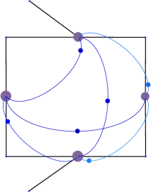
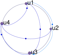
Figure 9: Synergies in a loop-shaped pathway (see Figure 6). (a) Network structure and reference flux (arrows). (b) Synergies between enzyme rhythms. Enzymes are shown as nodes, enzyme synergies as arcs with dots. Absolute values are indicated by arc colors (dark: large); phase shifts are marked by dots. Dots do not show actual oscillation phases but desired phase shifts that would maximise fitness. A dot’s position on the arc represents the phase shift in radians (units of $2\,\pi$): a dot near the end of an arc indicates a small phase shift and shows that the nearby node should peak after the more distant node (e.g. the arrow head between $u_{1}$ and $u_{2}$ shows that $u_{1}$ should peak slightly before $u_{2}$). A dot in the middle of an arc indicates that two enzymes should have opposite phases (like, e.g. $u_{1}$ and $u_{3}$). Self-synergies are not shown. (c) Synergy phase plot. Enzymes are placed on a circle, indicating their optimal phases. Arcs are drawn as in (b).

We saw how optimal enzyme rhythms in a given metabolic model can be computed. The formulae are summarised in the appendix and examples are shown at www.metabolic-economics.de/enzyme-rhythms/. However, can these formulae also explain general phenomena such as coregulation of enzymes or their sequential activation in pathways? To understand optimal enzyme profiles, and how they are shaped by fitness objectives, external conditions, metabolic dynamics, and enzyme constraints, numerical simulations alone are not enough – we need general laws that explain how enzyme rhythms – assuming small-amplitude, sine-wave oscillations – are shaped by fitness synergies and constraints on individual enzyme amplitudes. There are three types of synergies: environment/enzyme synergies (${\bf F}_{\rm\tilde{x}\tilde{e}}$), enzyme/enzyme synergies (${\bf F}_{\rm\tilde{e}\tilde{e}}$ off-diagonal elements), and enzyme self-synergies (${\bf F}_{\rm\tilde{e}\tilde{e}}$ diagonal elements). Synergies often reflect the fact that the actions of two parameters converge towards a common objective. They can emerge in different ways, for example: (i) Synergy via supply. A rhythm (in the environment or of an enzyme) leads to oscillations in a metabolite somewhere in the network. Since an enzyme that consumes this metabolite becomes more efficient in certain moments in time, there is an incentive to synchronise enzyme and substrate, thus coordinating the enzyme with the original oscillating parameter with the right phase delay. (ii) Synergy through a common target: for example, two enzymes have control over the two substrates of a reaction, creating a synergy effect; different “temporal distances” from the target reactions lead to synergies with different phase shifts. (iii) Synergy via avoidance. Metabolic rhythms can contain time windows in which certain processes would be inefficient or even dangerous (for instance, phases in which reactive oxygen species (ROS) levels are high, which makes DNA replication problematic). These processes should be shifted to other phases. (iv) Synergy via cost. If we assume a fixed total enzyme amount in each moment, then upregulating an enzyme implies a simultaneous downregulation of others. Similarly, in models with nonlinear enzyme cost functions, the upregulation of an enzyme may increase the cost pressure on other enzymes, creating an incentive for their downregulation. In both cases, a rhythm in one enzyme will promote rhythms in others, typically rhythms of opposite phase. Of course, these are just examples: there are many other scenarios that lead to rhythmic parameter synergies, and therefore promote a network-wide rhythmic dynamics.

Optimal enzyme rhythms as a whole must be self-consistent: each enzyme curve must be optimally adapted not only to external substrate rhythms, but also to all other enzyme curves and to the resulting metabolite rhythms. If all the synergies are known, how can we determine the optimal pattern of oscillations? What are the optimal amplitudes and phase shifts of all enzymes? A network-wide enzyme rhythm entails positive and negative synergies between all pairs of variables. Each periodic synergy defines a optimal magnitude and an optimal phase shift, according to this single synergy term. Knowing the actual parameter amplitudes and phase shifts in given periodic state, we can translate this into positive or negative, strong or weak synergy effects. The optimal network-wide enzyme rhythm is determined by the sum of all these effects: maximising this sum (see Box 2) requires an optimal compromise, possibly under constraints, between the synergy terms. Computing an optimal network-wide rhythm from known pairwise synergies is like computing a network-wide dynamic state from known local interactions in a dynamical system. If a dynamical system, e.g. a kinetic metabolic model, is perturbed by external oscillations, the shape of the resulting internal oscillations depends on the effects of the external perturbations and on the system’s internal dynamics, a dynamics that also becomes visible, e.g. in damped oscillations after a short perturbation. In dynamical systems, global dynamics arises from local interactions. Mathematically, the local interactions between metabolites are described by a sparse Jacobian matrix $\mathbf{A}$, and the global behaviour following a perturbation $\Delta{\bf e}$ (e.g. propagating waves or steady-state changes) can be derived from this matrix by matrix inversion In kinetic models, enzymes, metabolites, and reactions are directly linked by stoichiometric coefficients and reaction elasticities, which form the Jacobian matrix. The inverse Jacobian, a non-sparse matrix, determines the periodic response coefficients, which describe the global behaviour (including the propagation of perturbations). The transition from local interactions to network-wide behaviour also exists in enzyme optimisation: we start from pairwise fitness synergies, the “local” economic effects between single enzymes (which are, nevertheless, outcomes of the “global”, network-wide metabolic dynamics). Then we compute the optimal enzyme profile, i.e. the orchestrated pattern of all enzyme curves, by a matrix inversion.

Synergies and optimal phase shifts in metabolic systems can be shown in a synergy plot (see Figure 9). In this plot, oscillating parameters (external metabolite and enzyme activities) are displayed on the network and pairwise synergies are represented by arcs. Similarly, in a synergy phase plot the enzymes are arranged in a circle, sorted by their optimal phase shifts. While these phase shifts do not maximise each of the synergy effects individually, at least each enzyme peaks in the optimal moment, given the other enzyme curves. In a “good” metabolic cycle, arcs point in clockwise direction, indicating that the phase shifts agree with the phase shifts promoted by individual synergy terms.

How can we understand or compute optimal network-wide enzyme rhythms? It is hard to predict them based on intuition alone. One reason is their required self-consistent behaviour, which is much harder to depict mentally than simple cause and effect. A way to understand self-consistent enzyme profiles is to view them as the result of a hypothetical planning process in a which we start with a first tentative solution which is then iteratively refined. An external parameter oscillation causes metabolic oscillations in the network. We can first naively assume that each enzyme level is adapted “locally” to its periodic substrate and product levels, as described in section 2.1. This yields a periodic profile for each enzyme. Of course, these enzyme profiles will cause a change in the metabolite profiles, these require further enzyme adjustments, and so on. If we consider this infinite number of adjustements, and if their infinite sum converges, we obtain a self-consistent, optimal enzyme rhythm. Mathematically, the matrix inversion in Eqs (7) and (8) is an effective way to compute this infinite sum (see SI LABEL:sec:SIiterative). The same idea – describing a self-consistent enzyme adaptation strategy as an infinite sum of adjustments – can be applied to compute self-consistent static adjustments [17].

Generally, oscillations can be described by changes in time or by modes in frequency space. In time, the most simple perturbations are peak-like perturbations of single reactions. In a linearised metabolic dynamics, their propagation is described by the pulse-response function. The effects of general time-dependent perturbations can be described by convolution integrals. In this convolution, all the propagating effects are overlaid. If the perturbation itself is a sine wave the result (in a linear approximation) is a simple sine-wave dynamics as we saw before. Assuming sine waves as an ansatz for enzyme rhythms, allows us to describe rhythms simply by amplitudes and phases. In Fourier space, this corresponds to a multiplication of Fourier-transformed perturbation function with the Fourier-transformed pulse-response function. Thus, we can see the metabolic system as a filter, e.g. a low pass filter that damps high-frequency oscillations and lets slow oscillations and static changes pass through [21, 18].

For non-sine-wave perturbations, dynamic responses can be obtained by Fourier synthesis [18]. Based on our sine-wave approach, the dynamic (linearised) response can be computed by Fourier synthesis as an infinite sum over sine-wave responses of different frequencies. To do so, the input oscillations are approximated by a Fourier series of sine-wave oscillations with frequencies $0,\omega,2\,\omega,3\,\omega,..$. In practice, considering only the lowest harmonics often yields a good approximation. So how can we predict optimal adaptation in time? With our quadratic approximation Eq. (5) (symmetric against time shifts), and without constraints, the optimal enzyme amplitudes Eq. (8) are linear in the perturbation amplitudes, and independent between different frequencies: these solutions are completely additive. If desired, sine-wave adaptations to different sine-wave perturbations can be linearly combined, so we can apply Fourier synthesis: we split the perturbation profile into Fourier components, compute the respective optimal adaptations, and sum over them to obtain the optimal adaptation to the original, non-sine-wave perturbation (see SI LABEL:sec:HigherHarmonics). In contrast, if our optimality problem contains constraints (e.g. on enzyme amplitudes), this may not work: in this case, we need to solve Eq. (9), whose solutions may not be additive. In this case, blindly applying Fourier synthesis would lead to wrong results.

3.2 Periodic economic potentials

Optimal metabolic cycles require a self-consistent choice of the enzyme profiles, with the right amplitudes and well-synchronised peaks in time. While such arrangements look plausible once we see them, they may be hard to predict from intuition alone. The calculation via a matrix inverse in Eq. (8) is possible, but hard to grasp intuitively, and the entire network needs to be known. In our one-reaction example (see Box 1), things were much easier: the optimal enzyme profile was directly obtained from a local variable, the time-dependent catalytic rate, which results from the known substrate and product profiles. Can we find a similar local description for the entire network, one in which each enzyme adjusts is locally adjusted to substrate availabilty and product demand, described as “economic values”? Of course, these values would change periodically and would be coupled across the network. For example, if the product P of a pathway is useful in a certain cell cycle phase, it should peak in this phase. Therefore, the producing enzyme, and the enzyme’s substrate, should also oscillate, but peak a bit earlier. If we continue with this reasoning, and translate the “should” again into values, we find that each metabolite, and each enzyme, has a value that oscillates in time, and that all these values are interdependent. If the periodic values of metabolites (i.e. the incentives to produce them) are known, we may expect that an enzyme level should peak when substrate is cheap and product is pricy. With this concept, enzymes would adapt themselves locally, not to the concentrations but to the values of their reaction substrates and products, showing the highest investments when the value difference is large. Can we translate this idea into mathematical definitions and laws? This is in fact possible. Metabolic value theory [23] translates network-wide fitness objectives into economic proxy variables (assigned to individual reactions, metabolites, and enzymes, and describes these variables by local balance equations. In [24], economic values for metabolite production, called economic potentials, have been defined for steady and periodic states. For details, see SI section D. To describe oscillating states, we can consider complex-valued economic potentials, with phase angles describing when a metabolite’s value is highest.

4 Principles of optimal adaptation

4.1 Metabolic control, optimality, and portrayal relations

To model optimal enzyme rhythms, we combined dynamic metabolic models with optimality problems for enzyme profiles. Metabolic models, on the first level, imply a logic of cause and effect: enzyme perturbations affect reaction rates, changes in reaction rates affect metabolite concentrations, metabolite concentrations affect other reaction rates, and so on. On the second level, in the search for optimal enzyme profiles, we turn this logic around. Starting from an objective (at the end of our causal chains), we go back to metabolic states that support this objective and enzyme profiles that support these states. Requiring an optimal objective value and going back from objective to enzyme profiles, we trace all effects in reverse, from effect to cause, along pathways and in time. This inverse causation is called “promoting”: “promoting a rhythm” does not mean “causing a rhythm machanistically”, but “creating the incentive for a rhythm”. Any dynamical “forward” effects can be reflected in “reverse” incentives. For example, if an oscillating external nutrient is said to “promote” a periodic expression of a transporter, this simply mean that the transporter works more efficiently if expressed periodically in phase with its substrate. Any process that is influenced by an enzyme (either directly or indirectly) can promote adaptations of that enzyme. Importantly, for an enzyme A to promote enzyme B, no causal connection between them is needed. It suffices that A and B influence a third, fitness-relevant process C synergistically. Thus, metabolic value theory can be seen as an inversion of metabolic control. While MCT consideres enzymes and predicting their effects in forward direction, we start from desired effects and ask which enzyme adapatations might realise this effect in an optimal way. This is not new: it has been used to predict adaptation of steady states [17]. When we study optimal rhythms, this logic of a causal inversion seems even more apt because metabolite waves caused by an oscillating enzyme propagate visibly through the network and can be traced back along pathways and in time. Therefore, any “forward” features of dynamics may be reflected “in reverse”, in the choice of optimal enzyme strategies.

Our theory of optimal enzyme profiles relates the metabolic effects of enzymes (i.e. their function) to their own regulation (e.g. regulation mechanisms that can realise optimal enzyme adaptations). Biochemically, it would be conceivable that protein expression patterns are completely unrelated to protein function (for example, assuming a hypothetical genome in which the regions are shuffled). However, it is known (and physiologically important) that protein expression patterns reflect the way in which proteins act in metabolic pathways or other cellular systems. The components of protein complexes are often coexpressed, while their order of expression in time reflects the order of complex assembly [25]. Likewise, enzymes involved in a metabolic pathway have been shown to be expressed according to their order along the pathway [15]. This coordinated activation reflects – or as it were, “portrays” – the metabolic network topology, even if metabolic network and enzyme regulation have evolved separately, and there is no reason for them to show similar patterns.

In an engineered control system, a “portrayal relationship” between the controller and the system under its control would not be surprising at all: for instance, in predictive control, the controller employs a model – a kind of “mental representation” – of the systems to be steered, to make its choices. For reliable predictions, the internal model needs to resemble the real system in all relevant aspects, and for good outcomes, the controller needs to employ a meaningful objective function. In this sense, the controller must “portray” both the system to be steered (and possibly its uncertain environment) and the optimality task. But how can such a portrayal relation emerge in biological networks that are not engineered, but “tinkered” by evolution? Whether cells have a “mental representation” of their environment is something that cannot be shown by scientific means. However, an evolutionary adaption leading to similar outcomes is well conceivable. The enzyme profiles in a cell (and the regulation systems behind them) may end up “portraying” the metabolic network, its tasks, and its environment to an extent to which this provides a selection advantage. Thus, a portrayal relation, “implicit” in the behaviour shown by the control system, may evolve because of a fitness advantage that it provides.

The fact that enzyme expression reflects enzyme function is not surprising if cells behave economically: if the components of a complex are not expressed in the right proportions, or if enzymes in a pathway are not expressed in the right temporal order, resources are wasted. The portrayal relation between function and regulation emerges because of an evolutionary advantage, and we can study this by optimality models. The theory of optimal enzyme profiles explains why enzymes in pathways should be co-expressed and that their regulation patterns should reflect their own flux control. Portrayal relations between enzyme profiles (our control variables) and metabolism (the system to be controlled) have been found for other cases of metabolic control. For example, Klipp and Heinrich have studied flux maximisation in metabolic models with a fixed total enzyme amount and have shown that the optimal (i.e. flux-maximising) enzyme activities are proportional to the enzymes’ scaled flux control coefficients, i.e. to the enzyme’s relative effect on the steady-state flux [26]. Similar result was obtained for adaptation of static enzyme levels [17]: optimal adaptation profiles reflect fitness synergies ( second-order metabolic response coefficients), which reflect metabolic network structure. According to this prediction, the more strongly an enzymes affects relevant state variables, and the cheaper its adaptation would be, the more strongly it should be adapted. In sequential activation strategies, as predicted in [14, 15], enzyme activation reflect the sequence of enzymes in a metabolic pathway.

The theory of optimal enzyme rhythms extends this to periodic behaviour and provides analytical formulae that suggest a portrayal relationship between network structure, a meaningful order of processes, and optimal enzyme phases and amplitudes. Now we found similar phenomena for enzyme rhythms: optimal rhythms show coordinated patterns, and their phase shifts portray the order of metabolic reactions in the network.

How does the “portrayal relationship” between a metabolic system and enzyme profile arise mathematically? For example, can we find a link between enzyme profiles and metabolic network structure in our mathematical formulae? The shape of an optimal enzyme rhythm depends on three aspects: on periodic perturbations present in the environment, on the way external and enzyme-driven perturbations propagate in the network, and on the importance of different state variables for cell fitness. In our formulae, the second and third aspect determine the synergy matrices. The second factor, how perturbations propagate, is described by periodic response and control coefficients. These coefficients are closely related to network structure. On the one hand, they follow by matrix inversion from the Jacobian matrix, which portrays the network by describing neighbourhood relations between metabolites. On the other hand, stoichiometric matrix, elasticity matrix, control coefficients are related through summation and connectivity theorems [27], which directly links network structure, metabolic control (in “forward direction”), and the shape of optimal enzyme rhythms (arising from incentives propagating in “reverse direction”). Thus, enzyme rhythms (and, more generall, temporal enzyme profiles) portray network structure as a result of two matrix inversions. The Jacobian matrix reflects the network topology; by inverting it, we obtain metabolic control coefficients, which play a role in defining the enzyme synergies; by inverting this synergy matrix, we obtain the optimal enzyme profiles.

4.2 Principles of optimal periodic behaviour

Should organisms in periodic environments behave homeostatically, or should they use existing environmental variations as opportunities, running different processes at different times? If biochemical processes follow an optimal temporal order, which of them should be synchronised or be separated in time? How should a metabolic cycle proceed? From an optimality perspective, organisms should do what improves their evolutionary fitness. For example, many trees lose their leaves in winter and many animals hibernate, consuming the storage compounds they produced in the warmer seasons. Wood production in trees varies between seasons, and also flux profileering is season-dependent. We can think of such yearly cycles as a whole, as processes under a selective pressures. We can think of daily rhythms (e.g. the varying glucose supply and demand in our body and its management of by the liver) in a similar way. The behaviour in each phase should be adapted to the environment and to the behaviour in the past and future phases.

To predict optimal metabolic behaviour in time, we may postulate different control strategies: “myopic” strategies (“In each moment, adapt optimally to the current conditions as if they wer static”), “scheduling” strategies (“Shift processes to times that provide the best external conditions”), or “self-consistent” strategies (“Arrange all processes optimally in time, such that no rearrangement could provide an advantage). Self-consistent strategies imply anticipation and a shaping of future conditions: the enzyme activities are not adapted “passively” to existing substrate levels (as suggested by “just-in-time production” or implemented by substrate activation). Instead, they actively shape the metabolite profiles, to create conditions under which enzymes act more efficiently. We can see anticipation at work in the optimal activation patterns in linear metabolic pathways (which was described as “just-in-time” adaptation): if all enzymes were activated immediately, most of them would have little substrate and would therefore act inefficiently, so converting most of the substrate into product would take very long. A sequential activation, in contrast, creates high levels of internal metabolites and high concentration gradients at specific times, and provides time windows in which individual enzymes are very efficient.

5 Discussion

Whether metabolic rhythms are a by-product of overshooting regulation or whether they have biological functions (e.g. to improve metabolic efficiency) is an open question. In order to argue for biological functions, we need to show that oscillations can provide an advantage. Here I adopted this view and asked, specifically, whether enzyme rhythms can provide metabolic benefits (e.g. an improved metabolic performance at a constant overall enzyme investment) that cannot be realised by static enzyme changes alone.

In models, we may study this question by optimising either the enzyme profiles themselves or the regulation mechanisms behind them. Previous studies were focused on regulation (e.g. optimising the kinetic constants in allosteric or transcriptional regulation): the optimisation resembles a simulated evolution in which mutations can introduce additional regulation edges, destroy edges, or modify their regulation strengths, and allow us to quantify the selection pressures on such mutations. These studies have shown that the resulting rhythms can improve metabolic performance. However, the exact functional reasons for enzyme rhythms – why certain enzyme rhythms are beneficial and how they should be orchestrated – remain unclear. To study how benefits arise precisely, the present theory predicts enzyme profiles independently of how they are realised, which makes it more general. Once these profiles are known, possible ways to realiss them by regulation mechanisms can be studied separately.

A theory of optimal enzyme profiles, as developed here, has multiple benefits. First, it highlights the importance of enzyme synergies. The synergy matrices show why there can be incentives for oscillations, even if the static enzyme activities have already been optimised. Second, the formulae tell us how transcriptional and posttranscriptional rhythms should be combined at different frequencies, and makes the logic behind this more transparent than numerical simulations would do. Third, the theory shows us that promoted and autonomous enzyme rhythms are closely related, and why. A metabolic system may benefit from self-promoting metabolic cycles: whenever there is a positive principal synergy at a finite frequency, the reference states will be fitness-unstable against certain enzyme rhythms. If enzyme rhythms can improve the system’s performance even in a constant environment, there is an incentive for self-promoting oscillations. Other systems may be fitness-stable against self-promoting enzyme rhythms, and require external rhythms to promote rhythmic enzyme adaptation. In fact, a single model may show both types of behavior depending on parameter choices. For example, a linear pathway with strong dilution may show self-promoting rhythms, while the same pathway with weak dilution shows only adaptive rhythms. This parameter-dependent switch between strategies can be seen as a bifurcation. However, it is not a bifurcation in the usual dynamical sense, but an “economic” bifurcation concerning the optimal choice of strategies.

The theory of optimal enzyme rhythms does not presuppose specific metabolic objectives, but allows modeller to define arbitrary objectives, as functions of metabolite concentrations and fluxes. For wild-type cells, a fitness function may score relevant output variables such as biomass production. In biotechnological applications, the objective may represent a production rate to be maximised. In any case, we choose a metabolic objective that scores steady state variables such as biomass production rate and translate it into a functional for scoring time courses. Here I proposed two types of fitness functionals. In the state-average fitness, the metabolic state is first averaged over time and the static fitness function is then applied to the time-averaged state: in this case enzymes must shift the average concentrations and fluxes to have an effect on fitness. With a fitness-average fitness (and using a nonlinear static fitness functions), the overall fitness depends not only on the average state, but also on temporal fluctuations around it. Both of the functionals are computed from time averages, but they reflect different assumptions about cellular time scales. There are also more general fitness functionals that average state variables on a time scale $\tau$ before evaluating the fitness.

Biological rhythms can be described as a sequence of discrete phases like sleep and wake. Similarly, metabolic rhythms have been modelled as a sequence of steady states with different enzyme profiles [28]. However, the real dynamics of metabolic cycles is continuous rather than abrupt: if metabolic rhythms are driven by gene expression, they are smooth on metabolic timescales (see SI LABEL:sec:geneexpression), and even sudden external perturbations are smoothened while propagating through the metabolic network. Accordingly, the theory describes smooth metabolic rhythms with small amplitudes. The focus on sine-wave functions has a number of reasons. In control theory, optimal control profiles in time can be computed by solving the Riccati equation, a differential equation that is integrated backwards in time, starting from the final system state. To describe periodic behaviour, the initial and final states would have to be matched, which is difficult. However, an elegant way to do this is to Fourier-expand all curves and to convert the problem into an optimisation of the Fourier coefficients. This is what I did here: rhythms are described by smooth, small-amplitude sine-wave oscillations around a (possibly shifted) static reference state, with amplitudes, phases, and average shifts to be optimised. Eqs (7) and (8) show how an orchestrated enzyme behaviour can emerge from fitness synergies between the sine-wave profiles of single enzymes. Finally, in models without active constraints, Fourier synthesis also enables us to handle periodic perturbations other than sine waves.

A theory of optimal rhythms in networks can be useful in biological and medical modelling. In the human body, physiological states vary considerably between day and night, entailing substantial changes in enzyme expression. To better understand these changes – for example, glucose management by the liver – one may study how periodic enzyme activities affect metabolic dynamics and what quantitative benefits result from them. Similar models may be used to find optimal schedules for drug administration, or to plan combination therapies in which several drugs are given at different times, creating periodic blood profiles, to exploit allosynchrony. For example, a first drug could make cells more susceptible to a second drug, which is administered with a phase delay. To model this, we may use a mechanistic pharmacokinetics/pharmacodynamics model that describes the distribution and effects of drugs in the body. The control variables in this case would be drug dosages as time curves (instead of enzyme activities), and the aim would be to maximise an intended effect while minimising the side effects. Of course, with a simulation model at hand, optimal interventions can be determined by numerical optimisation of time curves. However, with a large number of control variables this may be hard, and starting from a good initial solutions (obtained from our perturbation theory) may be helpful. Moreover, general formulae may provide additional insights, for example about the roles of synergies and how they can be arranged in beneficial cycles. Such an abstract perspective may reveal characteristic patterns, or a “style” of optimal cycles. A theory of optimal rhythms can also clarify the relation between network structure, biochemical dynamics, and external interventions, from small pathways to larger networks. It shows how network-wide behaviour emerges from local fitness synergies, it thereby reveals general design principles behind enzyme rhythms, for example, the general conditions for self-promoting beneficial oscillations.

Appendix A Forced metabolic oscillations

To understand how enzyme rhythms can provide benefits, we first need to see how their effects propagate in metabolic networks. Here I summarise formulae from [17] and [18], using complex-valued vectors as explained in SI section LABEL:sec:SInotation. A kinetic model describes metabolic dynamics by rate equations ${\rm d}{\bf c}/{\rm d}t={\bf N}\,{\boldsymbol{\nu}}({\bf c},{\bf p})-\lambda\,{\bf c}$ with a concentration vector ${\bf c}$ (for internal metabolites), a stoichiometric matrix ${\bf N}$, and a flux vector ${\bf v}={\boldsymbol{\nu}}({\bf c},{\bf p})$ containing the rate laws $\nu_{l}({\bf e},{\bf c},{\bf p})=u_{l}\,k_{l}({\bf c},{\bf p})$. The term $\lambda\,{\bf c}$ describes dilution in growing cells with cell growth rate $\lambda$ (if dilution can be ignored, we set or $\lambda=0$). In models with conserved moieties [29], we can split the stoichiometric matrix ${\bf N}$ into a product ${\bf N}={\bf L}\,{\bf N}_{\rm R}$, where ${\bf N}_{\rm R}$ consists of linearly independent rows of ${\bf N}$, corresponding to independent internal metabolites. The vector ${\bf p}$ can contain two types of model parameters: externally defined parameters in a subvector ${\bf x}$ (e.g., external metabolite concentrations) and control variables in a subvector ${\bf e}$ (e.g. enzyme activities). A metabolic state with concentration vector ${\bf c}^{\rm st}$, satisfying the stationarity condition $0={\bf N}\,{\bf v}({\bf c}^{\rm st})$, is called a stationary state or steady state. For growing cells, the steady-state condition reads $0={\bf N}\,{\bf v}({\bf c}^{\rm st})-\lambda\,{\bf c}^{\rm st}$. To define a steady reference state, we consider a reference parameter vector ${\bf p}_{0}$ and require that all parameter sets ${\bf p}$ close to ${\bf p}_{0}$ lead to similar stable steady states ${\bf c}^{\rm st}({\bf p})$ (i.e. $p$ must not be close to a bifurcation point). Periodic parameter variations (i.e. of enzyme activities or external metabolite concentrations) are described by a time-dependent parameter vector

$${\bf p}(t) = {\bf p}_{0}+\mbox{Re}(\mbox{\rm e}^{i\omega t}\,{\tilde{\bf p}})$$ (10)

with a complex-valued amplitude vector ${\tilde{\bf p}}$ and circular frequency $\omega$ (see Figure A). The parameter rhythm leads to periodic concentration and flux changes that propagate through the network as damped waves. In a linearised model, the concentration and flux curves will be sine waves with frequency $\omega$. In nonlinear models, sine-wave perturbations can evoke higher harmonics and shift the average state. Here we neglect higher harmonics and focus on shifts of the average metabolite concentrations, fluxes, and metabolic fitness, which we study in a second-order approximation [18] (see Figure 2). These are the effects that matter for our fitness functions.

Box 3: Oscillations and complex amplitudes
Enzyme rhythms and their complex amplitudes. (a) Sine-wave oscillation of an enzyme level. Starting from a steady reference state (straight solid line), we shift the enzyme level by $\Delta\bar{e}$ and add a sine-wave oscillation with complex amplitude $\tilde{u}$ and circular frequency $\omega=2\,\pi/T$ (with period length $T$). In analogy to the notion of “cell cycle phases”, the rhythm can be divided into phases (maximal, decreasing, minimal, increasing), but here discrete phases are used only for illustration and have little importance in the present approach. Instead, we describe sine-wave oscillations by complex exponential functions ${\tilde{e}}\,\mbox{\rm e}^{i\,\omega\,t}$ and visualise them by rotating pointers. (b) The complex amplitude ${\tilde{e}}$ encodes oscillation amplitude and phase shift (phase at time $t=0$). The real part (projection to x-axis) describes the periodic deviation $\Delta\bar{e}(t)$. (c) Oscillations with different phase shifts (peak times shown by arrows). (d) The same oscillations, shown by pointers at time point $t=0$. (e) Peak times displayed on a “clock”: the vertical pointer corresponds to the curve that peaks at $t=0$; pointers for the other two curves follow in clockwise direction.

Oscillating metabolite and enzyme levels have direct effects on adjacent reaction rates. In a single reaction, if we assume that enzyme and metabolite concentrations are directly controllable, these effects can be described by spectral elasticities [18]. Since enzyme activities appear as prefactors in the rate laws ($v_{l}=u_{l}\,k_{l}({\bf c})$), an enzyme rhythm alone (at constant metabolite concentrations) cannot cause direct second-order effects (such as higher harmonics or shifts of the average flux). In contrast, metabolite rhythms or combined metabolite and enzyme rhythms can have such direct second-order effects (see SI Figure LABEL:fig:periodicelasticities). To see their effects on the average fluxes, we now consider two periodic parameters $a$ and $b$ (representing enzyme levels, metabolite concentrations, or other quantities affecting the rate directly). Their time profiles read

$$a(t)=\bar{a}+\mbox{Re}(\mbox{\rm e}^{i\omega t}\,{\tilde{a}}),\qquad b(t)=\bar{b}+\mbox{Re}(\mbox{\rm e}^{i\omega t}\,{\tilde{b}})$$ (11)

with complex amplitudes ${\tilde{a}}$ and ${\tilde{b}}$, frequency $\omega$, and phase difference $\Delta\varphi=\varphi({\tilde{a}})-\varphi({\tilde{b}})$. If $a$ peaks before $b$, the phase shift $\Delta\varphi$ is small and positive.

In metabolic control theory, the effects of small perturbations on reaction rates or steady states are described by sensitivities called elasticity, response, and control coefficients. In this article, unscaled sensitivities are used throughout. Let us first consider a single reaction. For small oscillations, the reaction rate reads approximately

$$v(t)\approx\bar{v}+E_{a}\,\Delta a(t)+E_{b}\,\Delta b(t)+\frac{1}{2}E_{aa}\,\Delta a(t)^{2}+E_{ab}\,\Delta a(t)\,\Delta b(t)+\frac{1}{2}E_{bb}\,\Delta b(t)^{2}$$ (12)

with reference flux $\bar{v}$ and reaction elasticities $E_{a},E_{b},E_{aa},E_{ab}$, and $E_{bb}$. The average flux shift due to the rhythms is given by

$$\Delta\langle v\rangle_{t}\approx\frac{1}{2}E_{\tilde{a}\tilde{a}}\,|\tilde{a}|^{2}+E_{\tilde{a}\tilde{b}}\,|\tilde{a}|\,|\tilde{b}|\cos(\Delta\varphi)+\frac{1}{2}E_{\tilde{b}\tilde{b}}\,|\tilde{b}|^{2},$$ (13)

with periodic second-order elasticities $E_{\tilde{a}\tilde{a}}=\frac{1}{2}E_{aa}$, $E_{\tilde{a}\tilde{b}}=\frac{1}{2}E_{ab}$, and $E_{\tilde{b}\tilde{b}}=\frac{1}{2}E_{bb}$. If parameter $a$ is an enzyme activity $u$ and parameter $b$ is a metabolite concentration $x$, the second-order elasticities are given by $E_{\tilde{a}\tilde{a}}=E_{\tilde{u}\tilde{u}}=0$, $E_{\tilde{a}\tilde{b}}=E_{\tilde{u}\tilde{x}}=\frac{1}{2\,u}E_{x}$, and $E_{\tilde{b}\tilde{b}}=\frac{1}{2}E_{xx}$, and we obtain a flux shift

$$\Delta\langle v\rangle_{t}\approx E_{\tilde{u}\tilde{x}}\,|\tilde{u}|\,|\tilde{x}|\cos(\Delta\varphi)=\frac{E_{x}}{2\,u}\,|\tilde{u}|\,|\tilde{x}|\cos(\Delta\varphi).$$ (14)

This formula resembles Eq. (3) (with $E_{\tilde{u}\tilde{x}}$ instead of the prefactor $k/2$). The second-order spectral elasticities describe synergisms between metabolite and enzyme rhythms, relating two rhythmic profiles to the resulting time average shift in reaction rate. Now we consider the entire network. Network-wide rhythms (caused by enzyme and external metabolite rhythms) can be described similarly, but with response coefficients instead of elasticities as expansion coefficients. Periodic response coefficients relate a sine-wave perturbation (of an enzyme or external metabolite) to the resulting flux and concentration rhythms (see SI LABEL:sec:ResponseFormulae). If a state variable $z$ (an internal concentration or metabolic flux) is influenced by oscillating parameters $a(t)$ and $b(t)$, a second-order expansion for $z(t)$ yields three kinds of effects: forced oscillations with frequencies $\omega$, forced oscillations with frequency $2\omega$, and a shift $\Delta\langle z\rangle_{t}$ of the average value. The shift consists of three terms:

$$\Delta\langle z\rangle_{t} \approx \frac{1}{2}~{}R^{\rm z}_{\rm{\tilde{a}}{\tilde{a}}}(\omega)~{}{\tilde{a}}^{2}+\frac{1}{2}R^{\rm z}_{\rm{\tilde{b}}{\tilde{b}}}(\omega)~{}{\tilde{b}}^{2}+\frac{1}{2}\mbox{Re}(\mbox{\rm e}^{-i\Delta\varphi}R^{\rm z}_{\rm{\tilde{a}}{\tilde{b}}}(\omega))~{}|{\tilde{a}}||{\tilde{b}}|.$$ (15)

The first two terms represent self-synergies of $a$ and of $b$ (describing, e.g. the dynamic self-inhibition of an enzyme); the third term describes a synergy between the parameters. Its magnitude and sign depend on the phase shift $\Delta\varphi$. Eq. (15) contains no first-order terms because the reference state (where ${\tilde{a}}={\tilde{b}}=0$) is an extremum point with respect to state shifts $\Delta\langle z\rangle_{t}$; it can be a minimum, a maximum, or a saddle point. In a model with many periodic parameters (amplitude vector ${\tilde{\bf p}}$), the total shift results from a sum over all pairwise synergies. We can generalise Eq. (15) and obtain

$$\Delta\langle z\rangle_{t} \approx \frac{1}{2}~{}{\tilde{\bf p}}^{\dagger}\,{\bf R}^{\rm z}_{\rm{\tilde{p}}{\tilde{p}}}(\omega)~{}{\tilde{\bf p}}.$$ (16)

The symbol ${\tilde{\bf p}}^{{\dagger}}$ denotes the adjoint vector (i.e. the complex conjugate transpose). The synergy matrix ${\bf R}^{\rm z}_{\rm{\tilde{p}}{\tilde{p}}}(\omega)$ can be computed from the stoichiometric matrix ${\bf N}$ and from the first-and second-order elasticities (see SI LABEL:sec:periodicdynamics). It is Hermitian and its matrix elements, called second-order periodic response coefficients (see SI LABEL:sec:ResponseFormulae), are equal to the second-order spectral control coefficients in [18] except for a scaling factor. In our second-order approximation, rhythms of different frequencies have no fitness synergies between them.

Figure 10: Optimality problem for enzyme rhythms. A metabolic state (with fluxes ${\bf v}$ and metabolite concentrations ${\bf c}$ as state variables) is controlled by external parameters and enzyme levels ${\bf e}$. The fitness function ${\mathcal{F}}$ is defined as the difference of metabolic objective $y$ and enzyme cost $h$. The need to maximise fitness creates an incentive for enzyme profiles with high benefit and low cost. The same scheme applies to optimal steady states (with static external and enzyme profiles) and optimal dynamic behaviour (with external and enzyme rhythms).

Appendix B Fitness functions for dynamic metabolic states

To define what we mean by optimal enzyme profiles, we need to refer to a given fitness objective. Our fitness objectives consist of two terms: a cost for enzyme levels and a benefit term for metabolite concentrations and fluxes (see Figure 10). For a single reaction, we consider a metabolic objective function $y(u,x)=q(v(u,x))$ and a cost function $h(u)$ and define the fitness ${\mathcal{F}}(u,x)=q(u,x)-h(u)$. For a metabolic network, we consider a fitness function

$${\mathcal{F}}({\bf e})=\underbrace{y({\bf e})}_{q({\bf z}({\bf e}))}-h({\bf e})$$ (17)

with state variables in a vector ${\bf z}$ (containing flux vector ${\bf v}$ and concentration vector ${\bf c}$), scored by a benefit $y({\bf z})$, and a control vector ${\bf e}$ scored by a cost $h({\bf e})$. The choice variables $u_{l}$ may comprise enzyme activities and other variables, e.g. the dilution rate in growing cells [17]. In a pathway model, the functions $y({\bf z})$ and $h({\bf e})$ may describe how the pathway contributes to cell fitness as assumed by the modeller. Empirical protein cost functions can be obtained experimentally [30, 31] from the growth deficits after a forced expression of idle protein. In our models, the enzyme cost function must be an increasing (linear or nonlinear) function of the enzyme activities. In our perturbation theory, metabolic objective and cost functions are approximated by a second-order expansion

$$q({\bf z}+\Delta{\bf z}) \approx q({\bf z})+{\bf q}_{\rm z}\cdot\Delta{\bf z}+\frac{1}{2}\Delta{\bf z}^{\top}{\bf Q}_{\rm zz}\Delta{\bf z}$$

$$h({\bf e}+\Delta{\bf e}) \approx h({\bf e})+{\bf h}_{\rm e}\cdot\Delta{\bf e}+\frac{1}{2}\Delta{\bf e}^{\top}{\mathbf{H}}_{\rm ee}\Delta{\bf e},$$ (18)

where ${\bf q}_{\rm z}$, ${\bf Q}_{\rm zz}$, ${\bf h}_{\rm e}$, and ${\mathbf{H}}_{\rm ee}$ are gradients and curvature matrices of $q$ and $h$. In models with external parameters $x_{j}$ (e.g. external metabolite concentrations), the steady-state fitness

$${\mathcal{F}}({\bf e},{\bf x})=\underbrace{y({\bf e},{\bf x})}_{q({\bf z}({\bf e},{\bf x}))}-h({\bf e})$$ (19)

contains ${\bf x}$ as an additional argument. In static optimality problems, the control variables $u_{l}$ must be chosen to maximise $f({\bf e},{\bf x})$ at given external parameters $x_{j}$ and under all given constraints. The synergy matrices can be computed from the curvatures of the fitness function Eq. (19)

$${\bf F}_{\rm ex} = {\bf q}_{\rm z}^{\top}~{}{\bf R}^{\rm z}_{\rm xe}+{{\bf R}^{\rm z}_{\rm x}}^{\top}{\bf Q}_{\rm zz}{\bf R}^{\rm z}_{\rm e}$$

$${\bf F}_{\rm ee} = {\bf q}_{\rm z}^{\top}~{}{\bf R}^{\rm z}_{\rm xx}+{{\bf R}^{\rm z}_{\rm x}}^{\top}{\bf Q}_{\rm zz}{\bf R}^{\rm z}_{\rm x}-{\mathbf{H}}_{\rm ee}.$$ (20)

In enzyme-optimal states, the fitness gradient ${\bf f}_{\rm u}=(\partial{\mathcal{F}}/\partial e_{l})$ must vanish for all active enzymes $e_{l}$ and the synergy matrix ${\bf F}_{\rm ee}$ must have negative eigenvalues.

Now we consider such an enzyme-optimal state $({\bf x}^{\rm ref},{\bf e}^{\rm ref})$ as our reference state, apply periodic perturbations, and search for optimal adaptations of our enzyme profiles. We assume that all parameters show sine-wave oscillations around their reference values:

$${\bf x}(t) = {\bf x}^{\rm ref}+\mbox{Re}(\mbox{\rm e}^{i\omega t}\,{\tilde{\bf x}})$$

$${\bf e}(t) = {\bf e}^{\rm ref}+\mbox{Re}(\mbox{\rm e}^{i\omega t}\,{\tilde{\bf e}}).$$ (21)

In a second-order approximation, these perturbations will shift the average state and the average fitness. The time average of a state variable $z$ can be expanded, using Eq. (15), as

$$\langle z\rangle_{t} \approx z({\bf x}^{\rm ref},{\bf e}^{\rm ref})+\frac{1}{2}~{}{{\tilde{\bf x}}\choose{\tilde{\bf e}}}^{{\dagger}}\left(\begin{array}[]{ll}{\bf R}^{\rm z}_{\rm{\tilde{x}}{\tilde{x}}}(\omega)&{\bf R}^{\rm z}_{\rm{\tilde{x}}{\tilde{e}}}(\omega)\\ {\bf R}^{\rm z}_{\rm{\tilde{e}}{\tilde{x}}}(\omega)&{\bf R}^{\rm z}_{\rm{\tilde{x}}{\tilde{e}}}(\omega)\end{array}\right){{\tilde{\bf x}}\choose{\tilde{\bf e}}}.$$ (24)

To characterise possible enzyme profiles ${\bf e}(t)$ by a fitness score, we define a fitness functional. In state-average fitness functionals, we assume a slow realisation of fitness effects: the fitness function (17) is applied to the time-averaged state:

$${\mathcal{F}}^{\rm(S)}=q(\langle{\bf z}(t)\rangle_{t})-h(\langle{\bf e}(t)\rangle_{t}).$$ (25)

In fitness-average fitness functionals, we assume an immediate realisation of fitness effects: we evaluate the fitness function (17) in each moment and take the time average:

$${\mathcal{F}}^{\rm(F)}=\langle q({\bf z}(t))-h({\bf e}(t))\rangle_{t}.$$ (26)

There also exist more general functionals which evaluate fitness on a specific time scale. In a functional $F=\langle f(\int K(t-t^{\prime})\,{\bf z}(t^{\prime})\,{\rm d}t^{\prime})\rangle_{t}$, the state variables $z(t$) are convolved with a kernel function (temporal width $\tau$), a fitness function is applied, and the resulting fitness values are averaged over time. State-averaged and fitness-averaged fitness functions are special cases of this general functional. Given our fitness function (17) and type of functional (${\mathcal{F}}^{\rm(S)}$ or ${\mathcal{F}}^{\rm(F)}$), we can compute the fitness effects of parameter oscillations. Periodic perturbations of external concentrations $x_{j}$ and enzyme activities $u_{l}$ lead to fitness changes that can be approximated by a quadratic function of ${\tilde{\bf x}}$ and ${\tilde{\bf e}}$. The synergy matrices (containing curvatures of this quadratic function) can be computed from periodic response coefficients and fitness derivatives. For the state-average fitness ${\mathcal{F}}^{\rm(S)}$, Eq. (25), they read

$${\bf F}_{\rm\tilde{e}\tilde{x}}^{\rm(S)} = {\bf q}_{\rm z}^{\top}~{}{\bf R}^{\rm z}_{\rm{\tilde{e}}{\tilde{x}}}(\omega)$$

$${\bf F}_{\rm\tilde{e}\tilde{e}}^{\rm(S)} = {\bf q}_{\rm z}^{\top}~{}{\bf R}^{\rm z}_{\rm{\tilde{e}}{\tilde{e}}}(\omega).$$ (27)

For the fitness-average fitness ${\mathcal{F}}^{\rm(F)}$, Eq. (26), they contain additional terms:

$${\bf F}_{\rm\tilde{e}\tilde{x}}^{\rm(F)} = {\bf q}_{\rm z}^{\top}~{}{\bf R}^{\rm z}_{\rm{\tilde{e}}{\tilde{x}}}(\omega)+\frac{1}{2}\,({\bf R}^{\tilde{\rm z}}_{\rm{\tilde{e}}}(\omega))^{{\dagger}}{\bf Q}_{\rm zz}{\bf R}^{\tilde{\rm z}}_{\rm{\tilde{x}}}(\omega)$$

$${\bf F}_{\rm\tilde{e}\tilde{e}}^{\rm(F)} = {\bf q}_{\rm z}^{\top}~{}{\bf R}^{\rm z}_{\rm{\tilde{e}}{\tilde{e}}}(\omega)+\frac{1}{2}\,({\bf R}^{\tilde{\rm z}}_{\rm{\tilde{e}}}(\omega))^{{\dagger}}{\bf Q}_{\rm zz}{\bf R}^{\tilde{\rm z}}_{\rm{\tilde{e}}}(\omega)-\frac{1}{2}{\mathbf{H}}_{\rm ee}.$$ (28)

For slow oscillations ($\omega\approx 0$) we can approximate ${\bf R}^{\tilde{\rm z}}_{\rm{\tilde{x}}}\approx{\bf R}^{\rm z}_{\rm x}$, ${\bf R}^{\tilde{\rm z}}_{\rm{\tilde{e}}}\approx{\bf R}^{\rm z}_{\rm e}$, ${\bf R}^{\rm z}_{\rm{\tilde{e}}{\tilde{e}}}\approx\frac{1}{2}{\bf R}^{\rm z}_{\rm ee}$, and ${\bf R}^{\rm z}_{\rm{\tilde{x}}{\tilde{e}}}\approx\frac{1}{2}{\bf R}^{\rm z}_{\rm xe}$. Eq. (B) yields the same synergy matrices as Eq. (B), but with a prefactor of 1/2. This prefactor has a simple explanation: periodic synergy matrices do not describe static parameter shifts with a fixed sign, but alternating perturbations which realise only $\sqrt{1/2}$ of the maximal amplitude on average. This also holds in the theoretical limit $\omega\rightarrow 0$ (where oscillations are infinitely slow).

Appendix C Optimal enzyme profiles

To compute optimal enzyme profiles, we first need to know how small (static or periodic) variations of enzyme activities or external parameters affect fitness. According to formula (5), all relevant information is contained in the synergy matrices (B) and (B). Based on these matrices and assuming no further constraints on the enzyme profile, we obtain formulae for optimal enzyme profiles for a number of cases (see Figure 3 and Box 4).

Box 4: Mathematical scenarios for optimal enzyme rhythms
The diagrams show fitness landscapes and constraints for enzymes in a larger metabolic system. Axes show the average enzyme level $\bar{e}$ (x-axis) and amplitude $|{\tilde{e}}|$ (y-axis). The phase angle (not shown) is assumed to be optimised. (a) Unperturbed reference state and systems with static or periodic external perturbations. Optimum points are shown by red dots. Circles represent contour lines of the fitness function. Inaccessible regions are shaded in grey. Perturbations shift the fitness function, and the enzyme must be optimally adaptated to reach follow the new optimum. (b) A system in which an enzyme becomes active under periodic perturbations. In the reference state, constraints (diagonal lines) force the enzyme to be inactive. Upon a periodic perturbation (right), an enzyme rhythm provides an advantage despite the cost of increasing of the average level. (c) Enzyme rhythms realised by a joint differential expression and posttranslational modification. The x and y axis refer to expression levels. Diagonal lines depict constraints on protein profiles. On the left, the optimal rhythm can be realised by expression changes alone (same as in Fig (a), right). In the centre diagram (with a tighter constraint, e.g. due to higher frequency), only a suboptimal rhythm (outside the centre point of the fitness landscape) can be realised. On the right, we assume that the cell can modulate its enzyme activities by posttranslational modification. Now any enzyme amplitude can be realised, but at a certain cost (function depicted by diagonal lines); this is why the optimum deviates from the nominal maximum of the fitness landscape (centre of the circle). (d) Cases in which the reference state is fitness-unstable against enzyme rhythms. In the case on the left, the amplitude will increase until it hits a bound, leading to spontaneous oscillations. In the case on the right, the solution diverges. In reality, large enzyme levels would be costly. In a model, this may be captured by additional bounds on maximal enzyme activities (not shown).

1. Criterion for optimal steady states. In a model with constant external parameters $x_{j}$, a static enzyme profile ${\bf e}$ is an interior optimum of the fitness function $f$ if all enzyme activities $u_{l}$ are positive, the fitness gradient ${\bf f}_{\rm u}({\bf x},{\bf e})$ vanishes, and the synergy matrix ${\bf F}_{\rm uu}({\bf x},{\bf e})$ is negative definite (i.e. all eigenvalues are strictly negative). In this case, the parameter set $({\bf x},{\bf e})$ is called enzyme-optimal. In contrast, an enzyme profile is a boundary optimum if some of the enzyme activities vanish and have negative fitness slopes $\partial{\mathcal{F}}/\partial u_{l}<0$, while the others form an internal optimum.

2. Optimal adaptation to static external perturbations. Let $({\bf x}^{\rm ref},{\bf e}^{\rm ref})$ be an enzyme-optimal parameter set and $\Delta{\bf x}$ be a static perturbation of ${\bf x}^{\rm ref}$. A static enzyme change $\Delta{\bf e}^{\rm opt}$ is called an optimal adaptation to $\Delta{\bf x}$ if it leads to a new enzyme-balanced state $({\bf x}^{\rm ref}+\Delta{\bf x},{\bf e}^{\rm ref}+\Delta{\bf e}^{\rm opt})$. For small perturbations $\Delta{\bf x}$, the optimal adaptation can be approximated by [17]

   $$\Delta{\bf e}^{\rm opt}(\Delta{\bf x}) \approx {\bf A}^{\rm u}_{\rm x}~{}\Delta{\bf x}$$ (29)

   with the adaptation matrix ${\bf A}^{\rm u}_{\rm x}=-{\bf F}_{\rm ee}^{-1}\,{\bf F}_{\rm ex}$. The synergy matrices ${\bf F}_{\rm ee}$ and ${\bf F}_{\rm ex}$ are given by Eq. (B), and ${\bf F}_{\rm ee}$ is invertible because it stems from an enzyme-optimal reference state. Consider a single reaction as an example. The fitness function reads ${\mathcal{F}}(e,x)=q(e,x)-h(e)$. The optimality problem leads to a non-zero enzyme activity $\bar{e}^{\rm opt}(x)=\mbox{argmax}_{e}\,{\mathcal{F}}(e,\bar{x})$ (see SI LABEL:sec:ex1 for an example). Since the fitness function is negatively curved, any spontaneous variation around the optimal point would lead to a fitness loss. When the substrate level increases from $\bar{x}$ to $\bar{x}+\Delta\bar{x}$, the optimal enzyme activity also increases. The optimal adaptation profile

   $$\Delta\bar{e}^{\rm opt} \approx -{\bf F}_{\rm ee}^{-1}\,{\mathcal{F}}_{\rm ex}\,\Delta\bar{x}$$ (30)

   depends on the negative synergy ${\bf F}_{\rm ee}=\frac{\partial^{2}{\mathcal{F}}}{\partial\mbox{\rm e}^{2}}$ and positive synergy ${\bf F}_{\rm ex}=\frac{\partial^{2}{\mathcal{F}}}{\partial\mbox{\rm e}\,\partial x}$ in the reference state. An increase $\Delta\bar{x}$ would lead to a positive adaptation $\Delta\bar{e}^{\rm opt}$ and the fitness increases by

   $$\Delta{\mathcal{F}}={\bf F}_{\rm ex}\,\Delta{\bar{e}_{\rm opt}}\,\Delta\bar{x}+\frac{1}{2}{\bf F}_{\rm ee}\,\Delta\bar{e}_{\rm opt}^{2}=-\frac{1}{2}{\mathcal{F}}_{\rm ee}^{-1}\,{\mathcal{F}}^{2}_{\rm ex}\Delta\bar{x}^{2}>0.$$ (31)

3. Optimal adaptation to external oscillations. The optimal adaptation to an external rhythm can be computed similarly. With a perturbation frequency $\omega$ and amplitude vector ${\tilde{\bf x}}$, the optimal enzyme amplitude vector reads

   $${\tilde{\bf e}}^{\rm opt}({\tilde{\bf x}}) \approx \tilde{\bf{A}}^{\rm e}_{\rm x}~{}{\tilde{\bf x}}.$$ (32)

   The complex-valued, frequency-dependent adaptation matrix $\tilde{\bf{A}}^{\rm e}_{\rm x}=-{\bf F}_{\rm\tilde{e}\tilde{e}}^{-1}\,{\bf F}_{\rm\tilde{e}\tilde{x}}$ follows from the synergy matrices ${\bf F}_{\rm\tilde{e}\tilde{e}}$ and ${\bf F}_{\rm\tilde{e}\tilde{x}}$ for periodic perturbations (Eqs (B) and (B)).

4. Static fitness changes By inserting the adaptation vectors $\Delta{\bf e}^{\rm opt}$ or ${\tilde{\bf e}}^{\rm opt}$ into Eq. (5), we obtain the first-order fitness changes resulting from enzyme adaptation to static or periodic perturbations. For periodic perturbations ${\tilde{\bf x}}$, the fitness change is given by $\Delta{\mathcal{F}}={{\tilde{\bf e}}^{\rm opt\,{\dagger}}}\,{\bf F}_{\rm\tilde{e}\tilde{x}}\,{\tilde{\bf x}}=-{\tilde{\bf x}}^{{\dagger}}\,{\bf F}_{\rm\tilde{e}\tilde{x}}^{{\dagger}}\,{\bf F}_{\rm\tilde{e}\tilde{e}}^{-1}\,{\bf F}_{\rm\tilde{e}\tilde{x}}{\tilde{\bf x}}$.

5. Benefit from self-promoting oscillations. An enzyme rhythm ${\tilde{\bf e}}$ alone can change the fitness by

   $$\Delta{\mathcal{F}} \approx \frac{1}{2}\,{\tilde{\bf e}}^{\dagger}\,{\bf F}_{\rm\tilde{e}\tilde{e}}\,{\tilde{\bf e}}.$$ (33)

   Any vector ${\tilde{\bf e}}$ with a positive fitness change $\Delta{\mathcal{F}}$ represents a beneficial, “self-promoting” enzyme rhythm. This holds, for example, for all eigenvectors of ${\bf F}_{\rm\tilde{e}\tilde{e}}$ with positive eigenvalues. Since ${\bf F}_{\rm\tilde{e}\tilde{e}}$ is Hermitian, its eigenvalues are real-valued and its eigenvectors span the space of possible amplitude vectors. A self-promoting enzyme rhythm requires that the reference state be fitness-stable against static enzyme changes, but fitness-unstable against certain enzyme rhythms. This means: all eigenvalues of ${\bf F}_{\rm ee}$ must be negative, but at least one eigenvalue of ${\bf F}_{\rm\tilde{e}\tilde{e}}(\omega)$, for some non-zero frequency $\omega$, must be positive. What is the most profitable enzyme rhythm at a given frequency? The eigenvector ${\tilde{\bf e}}^{\rm opt}$ with the largest eigenvalue (called principal fitness synergy $\sigma(\omega)$) represents the best enzyme rhythm with a given norm $||{\tilde{\bf e}}||$. Its elements define amplitudes and phases of all enzymes. If there exist beneficial enzyme rhythms at different frequencies, those with the highest principal synergy $\sigma$ have the biggest selection advantage and are most likely to emerge in evolution. If the benefit is maximal at $\omega=0$, oscillations of finite frequency are dispreferred. If we consider large-amplitude oscillations, the optimal enzyme rhythms are not simply given by eigenvectors, but may also shaped by the amplitude constraints.

Optimal enzyme profiles can also be shaped by constraints.

1. Bounds for enzyme amplitudes The amplitudes $|{\tilde{p}}|$ of protein profiles $\bar{p}+\mbox{Re}({\tilde{p}}\,\mbox{\rm e}^{i\omega t})$ are constrained for several reasons (see Figure 7). (i) A protein amplitude cannot be larger than the average protein level (i.e. $|{\tilde{p}}|\leq\bar{p}$) because protein levels would become negative otherwise. (ii) A dynamic model of protein production and degradation (with degradation constant $\kappa$) yields the tighter constraint $|{\tilde{p}}|\leq\sqrt{\frac{\kappa}{\kappa+\omega}}\,\bar{p}$ (see SI LABEL:sec:geneexpression), which coincides with the previous constraint at frequency $\omega=0$ (see Figure 7 (a)). (iii) The time derivative of a protein concentration, ${\rm d}p/{\rm d}t=-{\tilde{p}}\,\omega\,\sin(\omega t)$, reaches its higherst negative value $-{\tilde{p}}\,\omega$ when the protein level is $\bar{p}$ and a degradation rate is $\kappa\,\bar{p}$. Since the rate of decrease cannot be bigger than the degradation rate, we obtain the constraint ${\tilde{p}}\leq\frac{\kappa}{\omega}\bar{p}$. (iv) Due to space restriction in cells, we can put a bound on the maximal protein level $\bar{p}+|{\tilde{p}}|$ and on the average level $\bar{p}$. With all these constraints, each protein amplitude $|{\tilde{p}}|$ has an upper bound ${\tilde{p}}^{\rm max}(\bar{p},\omega,\kappa)=\mbox{min}(\sqrt{\frac{\kappa}{\kappa+\omega}},\frac{\kappa}{\omega})\,\bar{p}$ or briefly $\gamma(\omega,\kappa)\bar{p}$. The maximal relative amplitude $\gamma(\omega,\kappa)={\tilde{p}}^{\rm max}/\bar{p}$ depends on frequency $\omega$ and effective degradation constant $\kappa$; at frequencies $\omega\gg\kappa$, it becomes very small.

2. The role of constraints in enzyme optimisation The fitness expansion formula Eq. (5) contains no synergy terms between enzyme rhythms and static changes, and no synergy terms between enzyme rhythms of different frequencies. If a temporal parameter perturbation consists of sine-wave oscillations of different frequencies, and if Eq. 7 applies, the optimal adaptations to these components should therefore be additive. However, this only holds if there are no constraints on the enzyme activities (i.e. if Eq. (9) applies), or if the overall solution (i.e. optimal enzyme rhythms, summed over all frequencies) respects all constraints (e.g. on maximal enzyme activities). In practice, we may proceed by first computing a preliminary solution by summing the solutions for individual frequencies. If this solution violates some constraints, we need to discard this solution and instead determine a solution containing all frequencies by applying a single joint optimisation with constraints.

3. Enzymes that only become active in periodic states If an enzyme is inactive in the reference state, then it cannot start oscillating unless its mean level also increases: the mean value must be at least as large as the amplitude, and the resulting cost can be seen as an effective “oscillation cost” proportional to the amplitude. In this case, our two optimality problems – static and periodic adaptation – cannot be treated separately: instead of Eqs (7) and (8), a constrained optimality problem Eq. (9) must be solved, even if the oscillations are very small. There are two possible cases: (i) The reference state is fitness-stable against enzyme oscillations and enzyme rhythms are promoted by external oscillations. (ii) The reference state is fitness-unstable against enzyme oscillations despite the effective oscillation cost; then, in our second-order expansion, due to the linear increase in metabolic objective, the resulting oscillations will increase until they hit the bounds for maximal enzyme activities or amplitudes.

4. Non-optimal enzyme profiles and the resulting fitness loss. If a cell fails to use an optimal enzyme profile, this leads to a fitness loss. The fitness loss can be quantified by Eq. (5) (see Figure 3 (c)). With a mismatch ${\tilde{\bf e}}^{\rm mis}={\tilde{\bf e}}-{\tilde{\bf e}}^{\rm opt}$ between actual and desired amplitude vector, the fitness difference reads

   $$\Delta{\mathcal{F}}^{\rm mis} \approx \mbox{Re}({\tilde{\bf x}}^{{\dagger}}\,{\bf F}_{\rm\tilde{x}\tilde{e}}\,{\tilde{\bf e}}^{\rm mis}+{\tilde{\bf e}}_{\rm opt}^{{\dagger}}\,{\bf F}_{\rm\tilde{e}\tilde{e}}{\tilde{\bf e}}^{\rm mis}+{\tilde{\bf e}}^{*{\dagger}}\,{\bf F}_{\rm\tilde{e}\tilde{e}}{\tilde{\bf e}}^{\rm mis})=\mbox{Re}({\tilde{\bf e}}^{*{\dagger}}\,{\bf F}_{\rm\tilde{e}\tilde{e}}{\tilde{\bf e}}^{\rm mis})$$ (34)

   (note that ${\tilde{\bf x}}^{{\dagger}}\,{\bf F}_{\rm\tilde{x}\tilde{e}}\ +{\tilde{\bf e}}_{\rm opt}^{{\dagger}}\,{\bf F}_{\rm\tilde{e}\tilde{e}}=0$ in the reference state). If a metabolic state is fitness-stable against enzyme rhythms, the synergy matrix ${\bf F}_{\rm\tilde{e}\tilde{e}}$ is negative definite, so Eq. (34) describes an actual loss.

Matlab code and models for optimal enzyme rhythms are available at www.metabolic-economics.de/enzyme-rhythms/.

Appendix D Periodic economic potentials

The shapes of optimal enzyme profiles can be understood using concepts from metabolic value theory [22, 24, 23, 32]. Following Eq. (5), we first expand the fitness function quadratically around a steady reference state. Assuming that our solution does not hit any constraints, the optimality conditions read

$$0 = \underbrace{{\bf y}_{\rm e}+\mathbf{W}_{\rm ex}\,\Delta{\bf x}+\mathbf{W}_{\rm ee}\,\Delta{\bf e}}_{\mathring{\bf w}_{\rm e}}-\underbrace{(\mathbf{h}_{\rm e}+{\mathbf{H}}_{\rm ee}\,\Delta{\bf e})}_{\mathring{\bf h}_{\rm e}}\qquad\mbox{Static changes}\,\Delta{\bf x},\Delta{\bf e}$$

$$0 = \underbrace{\tilde{\bf w}_{\rm e}+\mathbf{W}_{\rm{\tilde{e}}{\tilde{x}}}\,\Delta{\bf\tilde{x}}+\mathbf{W}_{\rm{\tilde{e}}{\tilde{e}}}\,\Delta{\bf\tilde{e}}}_{\mathring{\bf w}_{\rm{\tilde{e}}}}-\underbrace{(\tilde{\bf h}_{\rm e}+{\bf H}_{\rm{\tilde{e}}{\tilde{e}}}\,\Delta{\bf\tilde{e}})}_{\mathring{\bf h}_{\tilde{e}}}\qquad\mbox{Periodic changes}\,\Delta{\bf\tilde{x}},\Delta{\bf\tilde{e}}.$$ (35)

The terms ${\bf y}_{\rm e},\mathbf{W}_{\rm ex},\mathbf{W}_{\rm ee}$, .., denote first and second derivatives of our metabolic objective $q$ and cost function $h$ in the unperturbed reference state. The bracket terms $\mathring{\bf w}_{\rm e}$ or $\mathring{\bf w}_{\rm{\tilde{e}}}$ (called static or periodic enzyme values) and terms $\mathring{\bf h}_{\rm e}$ or $\mathring{\bf h}_{\tilde{e}}$ (called static or periodic enzyme prices), denoted by circle $\circ$ can be seen as derivatives too. Unlike the usual gradients ${\bf y}_{\rm e}$ and $\mathbf{h}_{\rm e}$ (or $\tilde{\bf w}_{\rm e}$ and $\tilde{\bf h}_{\rm e}$) defined in the reference state, they are gradients describing variations around an existing periodic state. With these enzyme values and prices, the optimality conditions in a periodic state, Eq. (D), can be simply written as

$$\mathring{\bf w}_{\rm e}=\mathring{\bf h}_{\rm e},\qquad\mathring{\bf w}_{\rm{\tilde{e}}}=\mathring{\bf h}_{\tilde{e}}.$$ (36)

Enzyme values and prices in periodic states can be defined more generally outside our quadratic approximation: for general periodic states, with metabolic objective and cost functionals $g(\bar{\bf e},{\tilde{\bf e}})$ and $h(\bar{\bf e},{\tilde{\bf e}})$, we define them as

$$\mathring{\bf w}_{\rm e}=\frac{\partial g}{\partial\bar{\bf e}},\qquad\mathring{\bf w}_{\rm{\tilde{e}}}=\frac{\partial g}{\partial{\tilde{\bf e}}},\qquad\mathring{\bf h}_{\tilde{e}}=\frac{\partial h}{\partial\bar{\bf e}},\qquad\mathring{\bf h}_{\rm e}=\frac{\partial h}{\partial{\tilde{\bf e}}}.$$ (37)

Again, the optimality conditions $\frac{\partial f}{\partial\bar{\bf e}}=\frac{\partial g}{\partial\bar{\bf e}}-\frac{\partial h}{\partial\bar{\bf e}}=0$ and $\frac{\partial f}{\partial{\tilde{\bf e}}}=\frac{\partial g}{\partial{\tilde{\bf e}}}-\frac{\partial h}{\partial{\tilde{\bf e}}}=0$ are given by Eq. (D). What can we learn from these optimality conditions? If our expansion point is an enzyme-optimal steady reference state, we know that ${\bf y}_{\rm e}=\mathbf{h}_{\rm e}$; and if our fitness functional is not explicitly time-dependent, we also obtain $\tilde{\bf w}_{\rm e}=\tilde{\bf h}_{\rm e}=0$. In this case, the first-order terms in Eq. (D) cancel out and can be ignored. Then, by solving for $\Delta{\bf e}$ and $\Delta{\bf\tilde{e}}$ we reobtain Eqs (7) and (8). If, in addition, the cost functional is linear (i.e. ${\mathbf{H}}_{\rm ee}=0$), then $\mathring{\bf h}_{\tilde{e}}$ will vanish and we obtain $\mathring{\bf w}_{\rm{\tilde{e}}}=0$ as a simple optimality condition. In other words: in the state with optimal enzyme rhythms, the periodic value of each enzyme must vanish. Intuitively, this means that no small variation of enzyme amplitudes or phases can improve (even change) the metabolic objective to first order.

What else can we learn from optimality condition (D)? If enzyme values are displayed on the network, their amplitudes and phases reflect the network structure: for example, enzyme values are related between adjacent reactions. To see this, we introduce similar economic variable for metabolite production, called economic potentials, with the following definition. The function $g$ describes the overall metabolic objective, evaluated in the periodic state of the model. Now, for each independent metabolite $i$, we consider a small virtual exchange flux $r_{i}^{\rm virt}$ producing this metabolite. The static and periodic economic potentials are defined as $w_{r_{i}}=\frac{\partial g}{\partial r_{i}^{\rm virt}}$ and $w_{\tilde{r}_{i}}=\frac{\partial g}{\partial\tilde{r}_{i}^{\rm virt}}$, for static and periodic variations of the exchange flux. As shown in SI LABEL:sec:SIProofPeriodicbalanceequations, the (static and periodic) prices and the (static and periodic) economic potentials of their metabolites are linked by the balance equation

$${\mathring{\bf h}_{\rm e}\choose\mathring{\bf h}_{\tilde{e}}} = {\mathring{\bf w}_{\rm e}\choose\mathring{\bf w}_{\rm{\tilde{e}}}}=\left(\begin{array}[]{ll}\mathring{\bf E}^{v}_{u}&\mathring{\bf E}^{v}_{\tilde{e}}\\ \mathring{\bf E}^{\tilde{v}}_{u}&\mathring{\bf E}^{\tilde{v}}_{\tilde{e}}\end{array}\right)^{\dagger}\,{\square{\bf w}_{\rm r}+{\bf b}_{v}\choose\square\tilde{\bf w}_{\rm r}+{\bf b}_{\tilde{v}}}$$ (40)

with effective elasticities $\mathring{\bf E}^{x}_{y}$ defined for the periodic state. Here $\square w_{r_{l}}$ denotes the economic potential difference along reaction $l$, and the (static and periodic) flux gains ${\bf b}_{v}$ and ${\bf b}_{\tilde{v}}$ are direct derivatives of the metabolic objective functional with respect to metabolic fluxes. If we expand the elasticity coefficients around our steady reference state, we obtain the formula

$${\mbox{\rm Dg}(\bar{\bf e})\,\mathring{\bf h}_{\rm e}\choose\mbox{\rm Dg}(\bar{\bf e})\,\mathring{\bf h}_{\tilde{e}}} = {\mbox{\rm Dg}(\bar{\bf e})\,\mathring{\bf w}_{\rm e}\choose\mbox{\rm Dg}(\bar{\bf e})\,\mathring{\bf w}_{\rm{\tilde{e}}}}=\left(\begin{array}[]{lr}\mbox{\rm Dg}(\mathring{\bar{\bf v}})&\mbox{\rm Dg}(\mathring{{\tilde{\bf v}}})\\ \mbox{\rm Dg}(\mathring{{\tilde{\bf v}}})&\mbox{\rm Dg}(\mathring{\bar{\bf v}})\end{array}\right)^{\dagger}{\square\mathring{\bf w}_{\rm r}+{\bf b}_{\rm v}\choose\square\mathring{\bf w}_{\rm\tilde{r}}+{{\bf b}_{\tilde{v}}}}$$ (43)

where $\bar{\bf e}={\bf e}^{\rm ref}+\Delta{\bf e}$ contains the average enzyme activities, $\mathring{\bar{\bf v}}={\bf v}_{\rm ref}+\mathbf{E}^{\rm v}_{\rm c}\,\Delta\bar{{\bf c}}+\mathbf{E}^{\rm v}_{\rm x}\,\Delta{\bf x}$ is the vector of fluxes in the average state, and $\mathring{{\tilde{\bf v}}}=\mathbf{E}^{\rm v}_{\rm c}\,\tilde{{\bf c}}+\mathbf{E}^{\rm v}_{\rm x}\,{\tilde{\bf x}}$. Eq. (40), for periodic states, shows that static and periodic economic variables may affect each other. Applying this formula to the reference state itself, we can set $\mathring{\bar{\bf v}}={\bf v}$ and $\mathring{{\tilde{\bf v}}}=0$ and obtain separate balance equations for static and periodic fitness values

$$\mathbf{h}_{\rm e} = {\bf y}_{\rm e}=\mbox{\rm Dg}({\bf v}/\bar{\bf e})\,[\square{\bf w}_{\rm r}^{\rm int}+{\bf b}_{v}]$$

$$\tilde{\bf h}_{\rm e} = \tilde{\bf w}_{\rm e}=\mbox{\rm Dg}({\bf v}/\bar{\bf e})\,[\square{\bf w}_{\rm r}^{\rm int}+{\bf b}_{\tilde{v}}].$$ (44)

If the cost function is not explicitly time-dependent, all periodic enzyme prices must vanish ($\tilde{\bf h}_{\rm e}=0$). For details, see SI LABEL:sec:SIProofPeriodicbalanceequations.

Appendix E Extensions of the theory

The theory of optimal enzyme rhythms can be extended to cover more general cases.

1. Other types of constraints. In Eq. (9) for optimal profiles $\Delta{\bf e}$ and ${\tilde{\bf e}}$, we may consider extra constraints on metabolite concentrations, fluxes, the sum of enzyme activities, or time averages of these quantities. Some of the periodic flux or metabolite profiles may even be predefined. In general, with constraints of the form $\mathbf{M}\,{\tilde{\bf x}}=\tilde{\bf a}$, we can predefine linear combinations of periodic fluxes or concentrations. Alternatively, soft constraints can be implemented by penalty terms in the fitness function.

2. Other control variables. The control variables $u_{l}$ in our example models represent enzyme activities, whereas state variables $s_{i}$ represent metabolite concentrations. In other models, however, the variables can have different meanings. Enzyme levels may also be described as dynamic variables, while other quantities, such as mRNA levels, transcription factor activities, drug dosages, or cell growth rate (which determines dilution in metabolism) could be treated as control variables.

3. Frequency-dependent cost. Apparent enzyme costs in bacteria can be defined as the observable growth deficits after an overexpression of protein. In experiments, protein overexpression evokes a strong initial growth deficit, which decreases after some hours [31]: possibly, ribosome levels or other cellular resources get out of balance and the cell needs time to return to a balanced state. What if the same adjustments occur during slow metabolic oscillations? This would imply higher costs whenever enzyme levels are changing. Enzymes oscillations would be costly, and fast oscillations even more, because ribosome adaptation will be harder to achieve at high frequencies. To model this extra cost, we may assume frequency-dependent enzyme cost functions. However, when biological rhythms are slow and predictable (e.g. day-night cycles), cells may be able to anticipate and regulate ribosome demands, and no frequency-dependent cost needs to be assumed.

4. Periodic fitness functions So far we assumed fitness functions that do not explicitly depend on time: time dependencies are caused by parameter oscillations only. However, time-dependent fitness functions may be a reasonable assumption. Consider a pathway within in a large metabolic network and assume that the cell lives in a periodic environment. With optimally adapted enzyme profiles, all cellular subsystems will oscillate, and the requirements for our pathway product change periodically. To model our pathway alone, while capturing these periodic external demands, we need an effective time-dependent fitness function for our pathway. This is a general principle: whenever we like to use models to “zoom” into a system, we need be describe subsystems by separate effective models. Within these models, we need to allow for periodic fitness functions, which breaks the time-shift invariance of our fitness functionals, and new terms may appear in the fitness expansion Eq. (5): there can be first-order terms scoring periodic enzyme activities as well as synergy terms linking static shifts and amplitudes, or linking rhythms of different frequencies.

5. Rhythms in protein modification and allosteric regulation. Enzyme rhythms driven by periodic gene expression have limited amplitudes, and at high frequencies the possible amplitudes become very small (Figure 7 (a)). To obtain larger amplitudes, enzyme activities can be modulated by enzyme phosphorylation, which can be steered much more quickly than gene expression (Figure 7 (b)-(d)). However, this comes at a cost. When an enzyme is periodically inhibited (or incompletely activated), its efficiency decreases on average. To keep the average enzyme activity at its original value, the average protein level must be increased, wich entails a cost. To account for this cost in the model, we distinguish between an enzyme’s concentration $p(t)$ (concentration of enzyme molecules, appearing in the enzyme cost function) and its activity $u(t)$ (concentration of enzyme molecules in the active state, which appears in the rate laws). To write the enzyme cost as a function of $u$ (instead of $p$), we follow a simple logic. If a desired enzyme amplitude can be realised by protein expression alone, the posttranslational regulation is not used, enzyme and protein curves are identical, and the enzyme cost is given by protein cost (setting $p=u$). In contrast, if the desired enzyme amplitude is too large and hits the constraints, we introduce an auxiliary variable $q_{l}=\max(0,|{\tilde{e}}_{l}|-{\tilde{p}}^{\max}(\bar{p},\omega))$, describing the difference between the desired activity amplitude ${\tilde{e}}_{l}$ and the maximal protein amplitude ${\tilde{p}}^{\rm max}_{l}$ (see Figure 7). Then, we reformulate the optimisation problem with $\bar{\bf e},{\tilde{\bf e}},\bar{\bf p},$ and ${\bf q}$ (see SI LABEL:sec:PosttranslationalCost). The resulting extra cost is proportional to the extra amplitude achieved by inhibition and may briefly be called “cost of posttranslational inhibition”.

6. Amplitude constraints and resulting Lagrange terms Optimal enzyme rhythms under constraints are described by Eq. (9). Active constraints are treated by Langrange multipliers, and instead of Eqs (7) and (8) we obtain (proof in SI LABEL:sec:RhythmConstraintsLagrange)

   $$\Delta{\bf e} = -{\bf F}_{\rm ee}^{-1}\,\left[{\bf F}_{\rm ex}\,\Delta{\bf x}-{\boldsymbol{\beta}}-\mbox{\rm Dg}({\tilde{\bf p}}^{\rm max}_{\rm rel}(\omega))\,{\boldsymbol{\gamma}}\right]$$

   $${\tilde{\bf e}} = -{\bf F}_{\rm\tilde{e}\tilde{e}}^{-1}\,\left[{\bf F}_{\rm\tilde{e}\tilde{x}}\,{\tilde{\bf x}}-\mbox{\rm Dg}\left(\frac{{\tilde{\bf e}}}{|{\tilde{\bf e}}|}\right))\,{\boldsymbol{\gamma}}\right].$$ (45)

   The signs of the Lagrange multipliers (in vectors ${\boldsymbol{\beta}}$ for the upper bounds on $\bar{e}_{l}$ and ${\boldsymbol{\gamma}}$ for the upper bounds on $|{\tilde{e}}_{l}|$) reflect different types of constraints: $\beta_{l}<0$ for inactive enzymes (with $\bar{e}_{l}=0$), $\beta_{l}>0$ for enzymes whose average value hits an upper bound, and $\beta_{l}=0$ otherwise. Likewise, $\gamma_{l}>0$ holds for enzymes with active amplitude constraints, and $\gamma_{l}=0$ otherwise. If no constraints are hit, all Lagrange multipliers vanish and we reobtain our solution formulae (7) and (8). Otherwise, each active constraint yields a new term, and each of these terms affects the profiles of all enzymes through the matrix multiplication. If an enzyme hits its amplitude constraint, there is a nonzero vector component in ${\boldsymbol{\gamma}}$ that couples $\Delta{\bf e}$ and ${\tilde{\bf e}}$. At high frequencies the extra term in the first equation goes to zero and the coupling can be neglected. In the second equation, the vector ${\tilde{\bf e}}$ appears on both sides. Thus, instead of computing ${\tilde{\bf e}}$ directly from the equation, a self-consistent solution needs to be found.

References

- [1] L. Nedbal, V. Brezina, F. Adamec, D. Stys, V. Oja, A. Laisk, and Govindjee. Negative feedback regulation is responsible for the non-linear modulation of photosynthetic activity in plants and cyanobacteria exposed to a dynamic light environment. Biochim et Biophs Act, 1607:5–17, 2003.
- [2] R.R. Klevecz, J. Bolen, G. Forrest, and D.B. Murray. A genomewide oscillation in transcription gates DNA replication and cell cycle. PNAS, 101(5):1200–1205, 2004.
- [3] D.B. Murray, M. Beckmann, and H. Kitano. Regulation of yeast oscillatory dynamics. PNAS, 104(7):2241, 2007.
- [4] P.T. Spellman, G. Sherlock, M.Q. Zhang, V.R. Iyer, K. Anders, M.B. Eisen, P.O. Brown, D. Botstein, and B. Futcher. Comprehensive identification of cell cycle-regulated genes of the yeast Saccharomyces cerevisiae by microarray hybridization. Molecular Biology of the Cell, 9:3273–3297, 1998.
- [5] R.J. Cho, M.J. Campbell, E.A. Winzeler, L. Steinmetz, A. Conway, L. Wodicka, T.G. Wolfsberg, G. Gabrielian, D. Landsman, D.J. Lockhart, and R.W. Davis. A genome-wide transcriptional analysis of the mitotic cell cycle. Molecular Cell, 2:65–73, 1998.
- [6] A. Papagiannakis, B. Niebel, E.C. Wit, and M. Heinemann. Autonomous metabolic oscillations robustly gate the early and late cell cycle. Molecular Cell, 65:285–295, 2017.
- [7] J. Wolf and R. Heinrich. Effect of cellular interaction on glycolytic oscillations in yeast: a theoretical investigation. Biochemical Journal, 345:312–334, 2000.
- [8] A. Goldbeter. Biochemical Oscillations and Cellular Rhythms: The molecular bases of periodic and chaotic behaviour. Cambridge University Press, Cambridge, 1996.
- [9] J.-F. Hervagault, J.G. Lazar, and J. Ross. Predictions of thermodynamic efficiency in a pumped biochemical reaction. PNAS, 86:9258–9262, 1989.
- [10] Y. Himeoka and K. Kaneko. Enzyme oscillation can enhance the thermodynamic efficiency of cellular metabolism: consequence of anti-phase coupling between reaction flux and affinity. Physical Biology, 13:2, 2016.
- [11] R. Machné and D. Murray. The Yin and Yang of yeast transcription: Elements of a global feedback system between metabolism and chromatin. PLoS One, 7(6):e37906, 2012.
- [12] B.P. Tu, A. Kudlicki, M. Rowicka, and S.L. McKnight. Logic of yeast metabolic cycle: Temporal compartmentalization of cellular processes. Science, 310:1152, 2005.
- [13] M. Rügen, A. Bockmayr, and R. Steuer. Elucidating temporal resource allocation and diurnal dynamics in phototrophic metabolism using conditional FBA. Sci Rep, 5:15247, 2015.
- [14] E. Klipp, R. Heinrich, and H.-G. Holzhütter. Prediction of temporal gene expression. Metabolic optimization by re-distribution of enzyme activities. Eur. J. Biochem., 269:1–8, 2002.
- [15] A. Zaslaver, A.E. Mayo, R. Rosenberg, P. Bashkin, H. Sberro, M. Tsalyuk, M.G. Surette, and U. Alon. Just-in-time transcription program in metabolic pathways. Nature Genetics, 36:486–491, 2004.
- [16] R. Heinrich and E. Klipp. Control analysis of unbranched enzymatic chains in states of maximal activity. J. Theor. Biol., 182(3):243–252, 1996.
- [17] W. Liebermeister, E. Klipp, S. Schuster, and R. Heinrich. A theory of optimal differential gene expression. BioSystems, 76:261–278, 2004.
- [18] W. Liebermeister. Response to temporal parameter fluctuations in biochemical networks. J. Theor. Biol., 234(3):423–438, 2005.
- [19] A. M. Reimers and A.C. Reimers. The steady-state assumption in oscillating and growing systems. Journal of Theoretical Biology, 406:176–186, 2016.
- [20] M.T. Alam, V. Olin-Sandoval, A. Stincone, M.A. Keller, A. Zelezniak, B.F. Luisi, and M. Ralser. Nat Commun, 2017.
- [21] B.P. Ingalls. A frequency domain approach to sensitivity analysis of biochemical systems. J. Phys. Chem. B, 108:1143–1152, 2004.
- [22] W. Liebermeister. Optimal metabolic states in cells. Preprint on bioRxiv: DOI:10.1101/483867, 2018.
- [23] W. Liebermeister. Metabolic economics in kinetic models. Preprint on arXiv.org: arXiv:1404.5252, 2014.
- [24] W. Liebermeister. The value structure of metabolic states. Preprint on bioRxiv: DOI:10.1101/483891, 2018.
- [25] S. Kalir and U. Alon. Using a quantitative blueprint to reprogram the dynamics of the flagella gene network. Cell, 117:713–720, 2004.
- [26] E. Klipp and R. Heinrich. Competition for enzymes in metabolic pathways: implications for optimal distributions of enzyme concentrations and for the distribution of flux control. BioSystems, 54:1–14, 1999.
- [27] R. Heinrich and S. Schuster. The modelling of metabolic systems. Structure, control, and optimality. BioSystems, 47:61–77, 1998.
- [28] A. Palinkas, S. Bulik, A. Bockmayr, and H.-G. Holzhütter. Sequential metabolic phases as a means to optimise cellular output in a constant environment. PLoS ONE, 10(3):e0118347, 2015.
- [29] C. Reder. Metabolic control theory: a structural approach. J. Theor. Biol., 135:175–201, 1988.
- [30] E. Dekel and U. Alon. Optimality and evolutionary tuning of the expression level of a protein. Nature, 436:588–692, 2005.
- [31] I. Shachrai, A. Zaslaver, U. Alon, and E. Dekel. Cost of unneeded proteins in E. coli is reduced after several generations in exponential growth. Molecular Cell, 38:1–10, 2010.
- [32] W. Liebermeister. Metabolic economics in flux analysis: the principle of local value production. Preprint on arXiv.org: arXiv:1404.5072, 2014.