Order-to-chaos transition in the hardness of random Boolean satisfiability problems

Abstract

Transient chaos is an ubiquitous phenomenon characterizing the dynamics of phase space trajectories evolving towards a steady state attractor in physical systems as diverse as fluids, chemical reactions and condensed matter systems. Here we show that transient chaos also appears in the dynamics of certain efficient algorithms searching for solutions of constraint satisfaction problems that include scheduling, circuit design, routing, database problems or even Sudoku. In particular, we present a study of the emergence of hardness in Boolean satisfiability ($k$-SAT), a canonical class of constraint satisfaction problems, by using an analog deterministic algorithm based on a system of ordinary differential equations. Problem hardness is defined through the escape rate $\kappa$, an invariant measure of transient chaos of the dynamical system corresponding to the analog algorithm, and it expresses the rate at which the trajectory approaches a solution. We show that for a given density of constraints and fixed number of Boolean variables $N$, the hardness of formulas in random $k$-SAT ensembles has a wide variation, approximable by a lognormal distribution. We also show that when increasing the density of constraints $\alpha$, hardness appears through a second-order phase transition at $\alpha_{\chi}$ in the random 3-SAT ensemble where dynamical trajectories become transiently chaotic. A similar behavior is found in 4-SAT as well, however, such transition does not occur for 2-SAT. This behavior also implies a novel type of transient chaos in which the escape rate has an exponential-algebraic dependence on the critical parameter $\kappa\sim N^{B|\alpha-\alpha_{\chi}|^{1-\gamma}}$ with $0<\gamma<1$. We demonstrate that the transition is generated by the appearance of metastable basins in the solution space as the density of constraints $\alpha$ is increased.

I Introduction

Constraint satisfaction problems arise in many domains of computer science, statistical physics, information theory and engineering, or even popular puzzles such as Sudoku. In these problems there are given $N$ variables, a set of constraints and the task is to assign values to the variables such as to satisfy all the constraints. One of the most studied constraint satisfaction problems is Boolean satisfiability (SAT) in which all the variables are Boolean ($x_{i}\in\{0,1\}$, $i=1,\dots,N$) and the constraints are logical statements with a unique truth value, involving these variables. The conjunction of these statements is called a formula, and the goal is choosing the variables such as to satisfy a given formula. According to a fundamental theorem of propositional calculus, every such formula $F$ can be converted into conjunctive normal form. In CNF a formula is expressed as the conjunction (AND, $\wedge$) of $M$ clauses $C_{m}$, $m=1,\ldots,M$, i.e., $F=\bigwedge_{m}C_{m}$ with each clause being a disjunction (OR, $\vee$) of literals (a literal is a variable $x_{i}$ or its negation $\neg x_{i}\equiv\overline{x}_{i}$) that make up the clause. Typical studies focus on $k$-SAT problems in which every clause contains $k$ literals. A simple example with $N=3$, $M=4$ is the set of clauses $C_{1}=(\overline{x}_{1}\vee\overline{x}_{2}\vee x_{3})$, $C_{2}=(x_{1}\vee\overline{x}_{2}\vee x_{3})$, $C_{3}=(\overline{x}_{1}\vee x_{2}\vee x_{3})$ and $C_{4}=(\overline{x}_{1}\vee\overline{x}_{2}\vee\overline{x}_{3})$. The solutions $(x_{1},x_{2},x_{3})$ that satisfy all four constraints are $\{(1,0,1),(0,0,0),(0,0,1),(0,1,1)\}$.

When there are only a small number of constraints, i.e., the constraint density $\alpha=M/N$ is small, the solutions are easily found and there are many of them. When $\alpha$ is large, it is easy to show that the formula cannot be satisfied by any assignment of the variables. However, when $\alpha$ has intermediate values, finding a solution, or even showing that one (or none) exists can be very difficult. $k$-SAT for $k\geq 3$ has been shown to be NP-hard, i.e., while any candidate solution can be tested to satisfy the formula in polynomial time (in $N$) there is no known algorithm that would find solutions (or show there aren’t any) in polynomial time (poly-time). It is also NP-complete Cook (1971); Garey and Johnson (1979), which means that all problems in the NP complexity class can be reduced in poly-time to $k$-SAT (Cook-Levin theorem) and thus the famous $P$ vs $NP$ question can be answered from studying $k$-SAT: a poly-time algorithm for $k$-SAT with $k\geq 3$ would imply that all problems in NP are tractable ($P=NP$), otherwise $P\neq NP$. For a visual introduction to the $P$ vs. $NP$ problem see for example Pvs , and for a general audience review see Fortnow (2009). $k$-SAT has major applications in artificial intelligence, electronic design, automation, error-correction, bioinformatics, protein folding, drug-design, etc. Although still open, the current strongly held belief is that $P\neq NP$, which means that there is no poly-time algorithm to find $k$-SAT solutions for all formulas for $k\geq 3$. Since NP-hard problems occur frequently in daily and practical situations, there has been a strong impetus to understand the nature of the hardness in such problems, as such an understanding may lead to better heuristic algorithms.

In an earlier study Ercsey-Ravasz and Toroczkai (2011) we opened a novel perspective on SAT problems by introducing a new algorithm, as a continuous-time dynamical system (CTDS) in form of coupled ordinary differential equations (ODEs), to solve SAT problems. This algorithm or analog solver is deterministic, without backtracks or restarts and it is qualitatively different from the other, discrete algorithms. Using this solver we were able to demonstrate that constraint satisfaction hardness translates into a transient chaotic dynamics in the continuous-time dynamical system of the solver. Note that the appearance of chaos correlating with complexity transitions seems to be a generic phenomenon, supported by observations also using other, heuristic methods to solve NP hard problems. Examples include iterated maps Elser et al. (2007) and the use of algorithms for finding the ground states of Potts spin-glass type Hamiltonians that emulate the NP-hard problem of community detection in networks Hu et al. (2012a, b). In Ref. Hu et al. (2012a) Hu et al. by map the spin glass Hamiltonian to a dissipative, continuous dynamical system, which was shown to behave chaotically in unsolvable regimes.

As our approach is deterministic and non-heuristic, also makes it possible to bring the methods of nonlinear dynamical systems and chaos theory to bear on constraint satisfaction problems. In particular, we have shown that an invariant of the dynamics, the so-called escape rate $\kappa$ is a good measure of hardness of individual SAT instances, which correlated surprisingly well with the subjective hardness ratings by humans on Sudoku problems Ercsey-Ravasz and Toroczkai (2012); this measure is the main subject of this paper. Note that the CTDS algorithm is incomplete: it will always find solutions if they exist, but if the instance is not satisfiable, then the dynamics will keep running forever. However, the CTDS does solve MAXSAT, i.e., finds solutions which minimize the number of unsatisfied clauses.

The paper is organized as follows. In Section II we present the analog SAT solver from Ercsey-Ravasz and Toroczkai (2011) and its properties relevant to the present study. In Section III we introduce the notion of escape rate as a SAT problem hardness measure and show that it goes through a phase transition in the random 3-SAT ensemble as the constraint density is increased; we also show that this transition is of second order, similar to the transition in Ising ferromagnets. Section IV presents an argument for the nature of this transition while Section V identifies its origin in the appearance of certain metastable structures in the solution space. Section VI shows that the same phenomenon holds for 4-SAT, followed by section VII, in which we demonstrate that 2-SAT does not present this chaotic transition. Section VIII is devoted to conclusions and discussions.

II An analog deterministic SAT solver

To solve SAT with a continuous-time dynamical system Ercsey-Ravasz and Toroczkai (2011) we first reformulate the problem in the space of $N$ continuous variables $s_{i}$, $i=1,\dots,N$, which can take any value in the interval $s_{i}\in[-1,1]$. Here $s_{i}=-1$ is associated with the Boolean variable $x_{i}$ being false ($x_{i}=0$) and $s_{i}=1$ to it being true ($x_{i}=1$). Let $\mathbf{C}=\{c_{mi}\}$ be an $M\times N$ matrix with $c_{mi}=0$ when the literal $i$ is missing from clause $C_{m}$, $c_{mi}=1$ if $x_{i}\in C_{m}$ and $c_{mi}=-1$ for $\overline{x}_{i}\in C_{m}$ (clauses containing both a variable and its negation are automatically discarded as they are always satisfied). The matrix $\mathbf{C}$ fully determines the formula $F$. One can think of the space $\bm{s}$ as an $N$-dimensional hypercube ${\cal H}_{N}$ with sidelength $2$, with the solutions to the formula $F$ lying in the corners of ${\cal H}_{N}$. The CTDS algorithm to be defined below will, however, be allowed to visit any point within ${\cal H}_{N}$ and on its boundary.

To every clause $C_{m}$ we associate an analog cost function $K(\bm{s})\in[0,1]$ via $K_{m}(\bm{s})=2^{-k}\prod_{i=1}^{N}(1-c_{mi}s_{i})$. For example, for the clause $x_{1}\vee x_{3}\vee\overline{x}_{9}$ we have $K(\bm{s})=(1-s_{1})(1-s_{3})(1+s_{9})/8$. Every such product has exactly $k$ non-trivial elements of the form $(1\pm s_{i})$, corresponding to those literals that are present in $C_{m}$. Clearly, if $x_{i}\in C_{m}$ ($c_{mi}=1$) the corresponding term is $(1-s_{i})$ and $K_{m}=0$ if and only if (‘iff’) $s_{i}=1$ (corresponding to $x_{i}$ being true). If $\overline{x}_{i}\in C_{m}$ ($c_{mi}=-1$) then the term is $(1+s_{i})$ and $K_{m}=0$ iff $s_{i}=-1$ (corresponding to $x_{i}$ being false, or the literal $\overline{x}_{i}$ being true). Thus $K_{m}(\bm{s})=0$ in those corners of ${\cal H}_{N}$, and only those, in which the corresponding Boolean variables $x_{i}$ satisfy $C_{m}$. We are searching for those corner points $\bm{s^{*}}$ in which all the $C_{m}$ clauses are satisfied, i.e., $K_{m}(\bm{s^{*}})=0$, $\forall m\in\{1,\dots,M\}$, constituting solutions to the formula $F$. Defining the energy function $V(\bm{s},\bm{a})$ associated with formula $F$ via $V(\bm{s,a})=\sum_{m=1}^{M}a_{m}K_{m}(\bm{s})^{2}$, we see that as long as $a_{m}>0$, $\forall m\in\{1,\dots,M\}$ we have $V(\bm{s^{*}})=0$ if and only if $\bm{s^{*}}$ is a solution to $F$. The $a_{m}>0$ are auxiliary variables and represent the weight of a clause in the formula; one can think of them as Lagrange multipliers. Thus, we are looking for the lowest/zero energy points of $V$. The search dynamics defined in Ercsey-Ravasz and Toroczkai (2011) is a combination of a gradient descent in $\bm{s}$-space with an exponential ascent in the auxiliary $\bm{a}$-space:

$$\frac{ds_{i}}{dt}=-\frac{\partial}{\partial s_{i}}V(\bm{a},\bm{s}),\;\;\;i=1,\dots,N$$ (1)

$$\frac{da_{m}}{dt}=a_{m}K_{m}(\bm{s}),\;\;\;m=1,\dots,M$$ (2)

with positive initial conditions $\bm{a}(0)>0$ (due to (2), their positivity is then preserved during the dynamics). As shown in Ercsey-Ravasz and Toroczkai (2011), this system will always find solutions when they exist, as the exponential drive will extract the dynamics from any local trap (with the exception of highly symmetric formulas $F$ at low $\alpha$, see the Supplementary Information section of Ercsey-Ravasz and Toroczkai (2011)), and drive the trajectory into one of the solutions. Note that all solutions $\bm{s^{*}}$ are attractive for the dynamics Ercsey-Ravasz and Toroczkai (2011). In Ercsey-Ravasz and Toroczkai (2012) we show that the dynamics is focused in the sense that the least satisfied clause (the one with the largest $K_{m}$ value) dominates $V$ and the dynamics drives exponentially fast the variables towards satisfying that clause, until another clause becomes dominant and so on. It is important to note that while the scaling of the analog time $t$ to find solutions is polynomial in $N$ Ercsey-Ravasz and Toroczkai (2011), in physical device implementations the $a_{m}$ variables represent voltages or currents and thus the energetic resources needed to find solutions will become exponential for hard formulas which, is of course necessary, assuming the strongly held belief P$\neq$NP. However, while one does not know how to generate time, we can generate energy (within limits), and thus systems like (1)-(2) become realistic candidates for SAT solving devices (analog circuits).

As a practical note, during simulations one does not have to wait until the trajectory approaches asymptotically a fixed point solution (the SAT solution). Because of the mapping, the Boolean variable $x_{i}$ has a unique truth assignment whenever $-1\leq s_{i}<0$ (false) or $0<s_{i}\leq 1$ (true), so every point $\mathbf{s}\in{\cal H}_{N}$ of the hypercube (inside and on the boundary) has a corresponding unique Boolean assignment. The SAT solution is in the corner of an orthant (and there is only one corner in an orthant), so there is no point waiting for the trajectory to asymptotically approach that corner, one can just simply check whether the assignment corresponding to that orthant is a solution (recall that checking is fast in NP).

It is often the case, especially for easy formulas that there are several solutions $\bm{s^{*}}$. The Hamming distance between two solutions (binary strings) is defined as the number of places in which the corresponding values of the bits differ. If two solutions are unit Hamming distance apart we say that they belong to a solution cluster. A solution cluster is therefore formed by solutions that can be connected through single-variable flips always staying within satisfying assignments. For example, if $(s_{1}^{*},s_{2}^{*},s_{3}^{*},...,s_{N}^{*})$ and $(-s_{1}^{*},s_{2}^{*},s_{3}^{*},...,s_{N}^{*})$ are both solutions, these are both part of the same cluster and in this case $s_{1}$ is called a free variable as its value is inconsequential to the solution, because the formula is satisfied by the other variables. For this reason, all points on the corresponding edge of the hypercube $(s_{1},s_{2}^{*},s_{3}^{*},...,s_{N}^{*})$ with $s_{1}\in[-1,1]$ have $V=0$ and the dynamics can be attracted to any point on this edge (see Ercsey-Ravasz and Toroczkai (2011), Supplementary Information Section A about attracting sets).

Another frequently discussed notion in the literature is that of a frozen variable. A variable is said to be frozen in a given cluster, if it takes on the same value for all the solutions within that cluster; as opposed to the free variable, its value is crucial for the existence of that solution cluster. In random $k$-SAT, or other ensembles of constraint satisfaction problems (such as $k$-coloring, locked occupation problems, etc.) the region of constraint density where the problems are hardest for most algorithms, are characterized by all solution clusters having an extensive fraction of frozen variables.

III A chaotic transition in the escape rate

For satisfiable formulas the solution is always found but the trajectory of the dynamics can be transiently chaotic. The harder the formula the longer these chaotic transients, and thus measures of transient chaos can be used to quantify the intrinsic hardness properties of individual formulas Ercsey-Ravasz and Toroczkai (2011, 2012). Transient chaos is a well-known phenomenon from the theory of nonlinear dynamical systems Tél and Lai (2008); Lai and Tél (2011), observed to occur in many physical systems, such as fluids Gorman et al. (1984); Sommerer et al. (1996); Peixinho and Mullin (2006); Hof et al. (2006), dielectric cavities Schwefel et al. (2004); Altmann (2009), microwave scattering Doron et al. (1990), electric circuits Heagy et al. (1994), mechanical systems de Paula et al. (2006); In et al. (1998), NMR lasers Jánosi et al. (1994) and chemical reactions Scott et al. (1991); J.Wang et al. (1994). Transient chaos is associated with the existence of a non-attracting chaotic set (repeller) in the phase space. It has recently been shown Motter et al. (2013) that in undriven dissipative systems the approach to equilibrium is governed by several transient chaotic saddles acting as effective, time-varying chaotic sets.

An important aspect of the CTDS is that it is a hyperbolic dynamical system Ercsey-Ravasz and Toroczkai (2011), i.e., starting a number $N(0)$ of trajectories from different initial conditions from the inside of a domain containing the chaotic set, the number $N(t)$ of trajectories that are still found within that domain after time $t$ is exponentially decaying in time: $N(t)=N(0)e^{-\kappa t}$. The decay rate, or escape rate $\kappa$ is an invariant characteristic of the chaotic set Kadanoff and Tang (1984a); Cvitanović et al. (2009) and it describes the average rate at which individual trajectories escape to the attractors (which might be simple attractors, chaotic attractors, or attractors at infinity). Alternatively, we can say that the probability of a typical trajectory not escaping to the attractor (in our case a SAT solution) until time $t$ decays exponentially Tél and Lai (2008); Lai and Tél (2011); Kadanoff and Tang (1984b): $q(t)\sim e^{-\kappa t}$. Fig. S9 in the Supplementary Information of Ref Ercsey-Ravasz and Toroczkai (2011) shows such a decay for our CTDS (1)-(2). Note that in our case $\kappa$ is a characteristic of the dynamical system (1)-(2), i.e., of a single formula $F$. One can think of the average lifetime $\tau\sim\frac{1}{\kappa}$ of chaotic transients as the expected solution time for a given solvable formula taken by our algorithm when started from a random initial condition.

It is important to note that in order to estimate the hardness of a formula, one does not need to wait until the trajectories actually find solutions, $\kappa$ can be estimated from the statistics of the trajectories within a domain inside the hypercube ${\cal H}_{N}$. Note that when measuring $\kappa$ we are launching many trajectories from random points from within this domain. The domain has to be large enough to contain a large fraction of the chaotic repeller set. For example, the domain ${\cal D}={\cal H}_{N}\cap{\cal S}(r)$, where ${\cal S}(r)$ is the $N$-sphere of radius $r=\sqrt{N-1+(k-1)^{2}/(k+1)^{2}}$ (where $k=3$ for $3$-SAT, see Fig. S2 in the Supplementary Information of Ercsey-Ravasz and Toroczkai (2011)), will have this property. It is well known from the dynamical systems literature Cvitanović et al. (2009); Lai and Tél (2011) that after the initial transient trajectories have left the domain, the remaining trajectories are longer lived and are sampling the chaotic set, before themselves also eventually leaving the domain. These trajectories are chaotic and experience the flow structure around the repeller and contribute to the value of $\kappa$. Although the chaotic set is an unstable set for solvable SAT problems, its existence is what hinders finding the solutions quickly. Thus, the difficulty or the hardness of the problem can be estimated from the statistics of the trajectories inside a large-enough domain in the hypercube, overlapping with the repeller.

To develop a better understanding of the generic properties of hardness as function of $\alpha$, researchers have studied properties of statistical ensembles of random formulas with a given $\alpha$. The simplest ensemble is the random $k$-SAT ensemble where the formulas are generated uniformly at random. This ensemble is the main focus of this paper, but there are also other, frequently studied ensembles such as $k$-XORSAT. In $k$-XORSAT a clause sets the sum of $k$ Boolean variables (no negation) modulo 2 to a given value (0 or 1); there are $M$ such clauses. Since $k$-XORSAT has a special linear structure, it can be solved in poly-time via Gaussian elimination, and thus $k$-XORSAT is in $P$. We will briefly discuss $3$-XORSAT in the light of the present studies, in Section VIII.

The ensemble picture and its similarity to spin-glass models, has attracted statistical physics methods from the theory of strongly disordered systems. In particular, replica symmetry and cavity methods made it possible to obtain a better description of the structure of the solution space Kirkpatrick and Selman (1994); Monasson and Zecchina (1996); Mezard et al. (2002); Achlioptas et al. (2005); Mézard et al. (2005a, b); Krzakala et al. (2007); Achlioptas (2008); Ardelius and Zdeborova (2008); Zdeborová and Mézard (2008). Using these statistical ensemble methods, sharp transitions were found in the thermodynamic limit ($N,M\to\infty$, $\alpha=const.$) as function of $\alpha$. These include the clustering (or dynamical) transition point $\alpha_{d}$ Mézard et al. (2005b); Krzakala et al. (2007); Achlioptas (2008), the freezing transition $\alpha_{f}$ Ardelius and Zdeborova (2008); Zdeborová and Mézard (2008), and the SAT/UNSAT satisfiability threshold $\alpha_{s}$ Kirkpatrick and Selman (1994) etc. It is in the range $\alpha\in[\alpha_{f},\alpha_{s}]$ where all known algorithms fail or take exponentially long to solve problems , however, recent numerical results indicate that backtracking survey propagation (BSP) can solve some problems efficiently within a range beyond the freezing transition, for 3-SAT Marino et al. (2015). Beyond $\alpha_{s}$ the probability for a random SAT formula to be solvable is exponentially small in $N$ and the solvable ones are hard.

In Ref Ercsey-Ravasz and Toroczkai (2011) we have shown that with increasing $\alpha$ the trajectories of the CTDS become chaotic at some transition density $\alpha_{\chi}$, with the nature of chaos changing with $\alpha$ towards, and past the SAT/UNSAT transition point $\alpha_{s}$. In this paper we present a more in-depth study of the behavior around $\alpha_{\chi}$ for $k=3$.

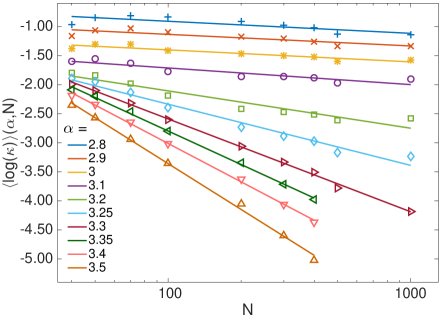
Figure 1: Ensemble averages of the escape rate $\kappa$ calculated on $J$ random instances, for fixed $\alpha$ as function of $N$, in logarithmic scale. The values of $J$ are given in the text.

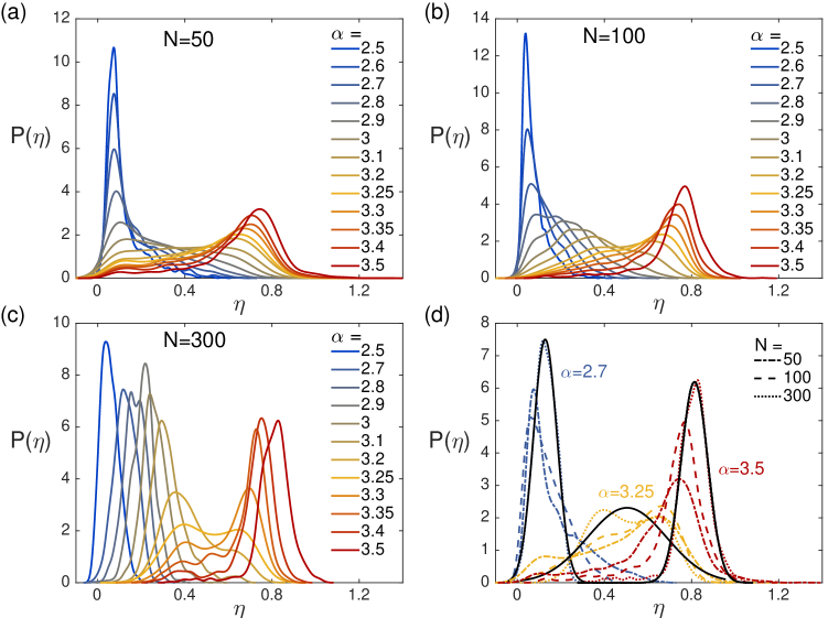
Figure 2: Normalized densities $P(\eta)$ of hardness for different $\alpha$ values for random satisfiable $3$-SAT formulas with a) $N=50$, b) $N=100$ and c) $N=300$. d) Gaussian fits to the $P(\eta)$ for $N=300$ at $\alpha=2.7$, $\alpha=3.25$ and $\alpha=3.5$, respectively. The distributions became increasingly sharper with increasing $N$. For a given $N$, when increasing $\alpha$ from smaller values towards larger ones the mean of the distributions shifts to larger values.

Let ${\cal E}(\alpha,N)$ denote the random 3-SAT ensemble of random formulas for fixed $\alpha$ and $N$. Let us denote by $p(t)$ the probability that a typical formula at $(\alpha,N)$ is not solved by time $t$ by our solver. Numerical evidence indicates the $p(t)$ behaves as $p(t)\sim e^{-\langle\kappa\rangle t}$, where the decay rate $\langle\kappa\rangle=\langle\kappa\rangle(\alpha,N)$ is the escape rate of a typical formula. It is easy to see that $p(t)$ is nothing but the average fraction of formulas from ${\cal E}(\alpha,N)$ that have not been solved by time $t$: the probability that exactly $j$ formulas have not been solved by time $t$ out of $J$ independently sampled ones is simply the binomial distribution $\binom{J}{j}p(t)^{j}[1-p(t)]^{J-j}$. Therefore, the average number of unsolved formulas by time $t$ is the average of the binomial, which is $Jp(t)$ and thus the average fraction of unsolved formulas is simply $p(t)$. In Ref Ercsey-Ravasz and Toroczkai (2011) we have shown that this fraction decays exponentially as $e^{-\lambda t}$ which means that $\langle\kappa\rangle=\lambda$. We have also shown that for hard problems (e.g., for $\alpha\geq 4.25$) and large $N$, the exponent $\lambda$ decays polynomially with $N$, i.e., $\lambda\sim N^{-\beta}$, where for example, for $\alpha=4.25$, $\beta\simeq 1.6$. Fig 1 shows that the power-law decay is true for other constraint densities $\alpha$ as well, albeit with an exponent that depends on $\alpha$. Fig 1 depicts the logarithm of the escape rate averaged over an ensemble $\langle\log(\kappa)\rangle(\alpha,N)$ as function of $N$, with $\alpha$ fixed, for several $\alpha$ values. In general, for a given $\alpha$ and $N$, $J=1000$ formulas were generated from ${\cal E}(\alpha,N)$ and for each formula we fitted a $\kappa$ value from typically $10^{3}-10^{4}$ trajectories started from random initial conditions.

As a consequence, the order of magnitude of $\kappa$ for individual formulas decays polynomially with $N$. Even though the ensemble averaged escape rate $\langle\kappa\rangle(\alpha,N)$ is well defined, it might be that the fluctuations around it are wide, which, as we will show below is actually the case. To better capture individual fluctuations but remove the leading $N$-dependence from the hardness measure we introduce a modified hardness measure, computable for an individual formula via:

$$\eta=-\frac{\log_{10}\kappa}{\log_{10}N}\;.$$ (3)

We next use this hardness measure and the finite-size scaling method from statistical mechanics (previously applied to SAT in Ref Kirkpatrick and Selman (1994)) to study the appearance of chaos in the behavior of the solver as function of $\alpha$. Note that definition (3) does not eliminate completely the $N$-dependence from the hardness measure, only to leading order.

First, we studied $3$-SAT problems for several values of $N\in[40,1000]$ and $\alpha\in[2.5,4.4]$ (see Fig.2). We measured $\eta$ of $J=1000$ (for $N\leq 200$), $J=500$ ($N=300,400$) and $J=200$ ($N=500,1000$) individual random satisfiable formulas. For each formula we ran the dynamics starting from $10,000$ (for $N\leq 200$), $5,000$ ($N=300,400$) and $2,000$ ($N=500,1000$) random initial conditions and estimated the escape rate $\kappa$, and consequently $\eta$. The corresponding distributions are shown in Fig. 2(a-c) for $N=50,100,300$. For small $\alpha$ the $P(\eta)$ distributions are sharp and concentrated around their average $\langle\eta\rangle(\alpha,N)$, but with increasing $\alpha$ the distributions seem to shift to the right, suddenly, becoming concentrated around a larger average value. For intermediary $\alpha$ values the distributions are wide and flat, see Fig 2(d). As function of $N$ the distributions become sharper for $\alpha$ away from $\alpha_{\chi}\simeq 3.28$ (where the distributions are flat), see Fig 2(d).

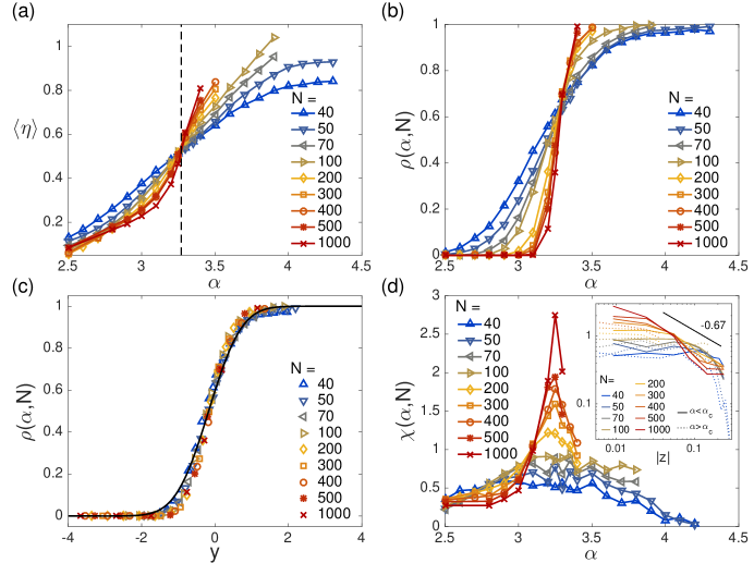
Figure 3: (a) Average formula hardness $\langle\eta\rangle(\alpha,N)$ as function of $\alpha$ for different values of $N$. The curves intersect at approximately $\alpha=3.28$ and $\langle\eta\rangle=0.5$. b) The fraction of problems $\rho$ with $\eta>\eta_{c}=0.5$ as function of $\alpha$. c) Rescaled $\rho$ curves using Eq (6) with $\nu=0.5$. The continuous black line is the fit $b\,\mbox{erfc}(-y-y_{0})$ with $b=0.5$ and $y_{0}=0.17$ . d) Susceptibility (4) as function of $\alpha$. The inset shows $\chi$ vs. $|z|$. The slope of the fit is -0.67, i.e., $\gamma=0.67$.

Plotting the average hardness defined by $\langle\eta\rangle(\alpha,N)=\int d\eta\,\eta P(\eta)$ as function of $\alpha$ for each $N$ we observe a critical point around $\eta_{c}\simeq 0.5$ and $\alpha_{\chi}\simeq 3.28$, where the curves intersect each other, shown in Figs. 3(a). As seen from Fig. 2(d), it is also around this point where the width of the distribution is the largest. While for large $N$ it is too costly to do the statistics for larger $\alpha$, at small $N$ this was done up to the satisfiability threshold. It shows that the hardness constantly increases with $\alpha$ and gets saturated somewhere above $\alpha=4.2$ near the SAT/UNSAT transition.

The behavior of the hardness around $\alpha_{\chi}$ has the hallmarks of a second-order phase transition from critical phenomena. In analogy with an Ising spin system, if $\alpha$ represents the level of “drive”, which is the external magnetic field $H$ in the Ising system, then the average hardness $\langle\eta\rangle(\alpha,N)$ is the system’s response, or magnetization per spin $M$ in the Ising model. Accordingly

$$\chi(\alpha,N)=\frac{\partial\langle\eta\rangle}{\partial\alpha}$$ (4)

(or $\frac{\partial M}{\partial H}$ in the Ising model) is the corresponding “magnetic” susceptibility. As one can see from Fig 3(d) and its inset the susceptibility diverges at $\alpha_{\chi}$ as

$$\chi\sim|z|^{-\gamma}\;,\;\;\;z\equiv\frac{\alpha-\alpha_{\chi}}{\alpha_{\chi}}\;,\;\;\;\gamma=0.67$$ (5)

from both sides. In Fig. 3(b) we plot the fraction $\rho$ of formulas with hardness $\eta>\eta_{c}=0.5$ as function of $\alpha$ for different $N$. Indeed, one can see that curves for different $N$ intersect each other around the critical value $\alpha_{\chi}$ and as $N$ increases the transition between the two phases becomes increasingly sharper. Plotting $\rho$ as function of the transformed variable:

$$y=N^{\nu}z$$ (6)

the curves can be made to fit on top of each other. The best fit is achieved with $\nu=0.5$.

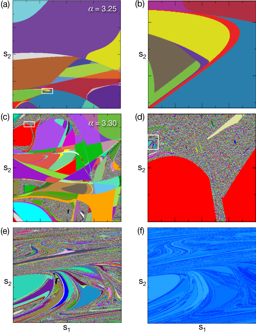
Figure 4: Projections of basins of attraction of solutions for a large random formula with $N=1000$ variables. (a) and (b) are at $\alpha=3.25$, just before the transition point $\alpha_{\chi}$, whereas (c-f) are at $\alpha=3.30$, just after $\alpha_{\chi}$. We fixed a random initial condition for all $s_{i},\,i\geq 3$ and varied only $s_{1}$ and $s_{2}$ on a $600\times 600$ grid. The points are colored according to the solution the dynamics flows to. In (a) and (c) both $s_{1}$ and $s_{2}$ span the range $[-1,1]$. (b) is a magnification of the region in the white rectangle from (a), (d) is the magnification of the region within the white rectangle from (c) and (e) is a magnification of the white rectangle from (d). (f) shows in shades of blue the time it takes to find the solution for every gridpoint in (e) with darker blue corresponding to longer times. Panels are not to scale.

To better interpret the observations above and the corresponding scaling exponents, we will model $P(\eta)$ with an effective, unimodal two-parameter distribution. We also use the observation that hardness is bounded from above, i.e., there exists a largest hardness saturation value $\eta_{max}$ (in the thermodynamic limit). As discussed earlier, the simulations shown in Ercsey-Ravasz and Toroczkai (2011) generated an exponent of $\beta=1.6$ for the hardest formulas. which implies that $\eta\leq\eta_{max}\simeq 1.6$ for all $\alpha$. Thus $P(\eta)$ is a distribution with a finite support $\eta\in(0,\eta_{max}]$. A simple choice is that of a truncated Gaussian url :

$$P(\eta)=\frac{A}{\sqrt{2\pi}\sigma}\,e^{-\frac{(\eta-\langle\eta\rangle)^{2}}{2\sigma^{2}}}$$ (7)

where $\langle\eta\rangle=\langle\eta\rangle(\alpha,N)$ is the mean and $\sigma=\sigma(\alpha,N)$ is the width/spread of the distribution. Using this form we can write:

$$\rho(\alpha,N)=\int_{\eta_{c}}^{\infty}d\eta\,P(\eta)=\frac{A}{2}\mbox{erfc}\left(\frac{\eta_{c}-\langle\eta\rangle}{\sqrt{2}\sigma}\right)$$ (8)

where $\mbox{erfc}(x)=\frac{2}{\sqrt{\pi}}\int_{x}^{\infty}dx\,e^{-x^{2}}$ is the complementary error function. The continuous black line in Fig 3(c) is a fit to a complementary error function $\sim\mbox{erfc}(-y-y_{0})$. Since the rescaled $\rho$ curves are well approximated by the erfc near the critical point, we can write:

$$y=N^{\nu}z=-\frac{\eta_{c}-\langle\eta\rangle}{\sqrt{2}\sigma}$$ (9)

or that

$$\sigma=\frac{|\eta_{c}-\langle\eta\rangle|}{\sqrt{2}N^{\nu}|z|}$$ (10)

Eq (10) shows that the hardness distribution within the ensemble scales as $1/\sqrt{N}$ with the number of variables $N$ (the numerator has a bounded variation). In terms of $\alpha$ (or $z$), the behavior is more complicated, as for $|z|\to 0$ we have $|\eta_{c}-\langle\eta\rangle|\to 0$ and the functional form depends on the depedence of $\langle\eta\rangle(\alpha,N)$ on $\alpha$. However, near the transition point we can write based on (5) that

$$|\eta_{c}-\langle\eta\rangle|\sim|z|^{1-\gamma},$$ (11)

and thus $\sigma\sim|z|^{-\gamma}$, i.e., diverges at the critical point, which is consistent with the sudden widening of the distributions seen in Fig 2. An interesting consequence of (10) is that near the critical point ($|z|\ll 1$) we have $P(\eta)=P(\alpha,N)=P(z,N)=\frac{A}{\sqrt{2\pi}\sigma}e^{N^{2\nu}z^{2}}$, i.e., $P\sim\sqrt{N}z^{\gamma}e^{Nz^{2}}$.

There are some caveats here. First, the density of the order parameter $\eta$, $P(\eta)$ is not necessarily a Gaussian, it was only approximated that way. E.g., in the 1D Ising model, although the distribution of the magnetization is unimodal and Gaussian-like, it is a complicated function (expressed with modified Bessel functions) Antal et al. (2004). A possible alternative for the limiting distribution could even be a generalized Gumbel-like pdf, which works well, for example, in the 2D XY model in a magnetic field, as shown by Portelli et al. Portelli et al. (2001). Second, because of normalization url , $A$ in (7) will also depend on $\langle\eta\rangle$, $\sigma$ and $\eta_{max}$, however, the dependence is fairly weak. From Fig 3 we find $A\simeq 1.2$ instead of $A=1$ which would be for a non truncated Gaussian. Third, the width of the distribution $\sigma$ at the critical point cannot diverge because the whole distribution is on a bounded support; however, this would be taken care of by the corrections to the Gaussian in the true form of $P(\eta)$.

IV Transient chaos for $\alpha\geq\alpha_{\chi}$

While numerical errors are inevitable when estimating the escape rates, the critical value $\eta_{c}=0.5$ has a deeper meaning.

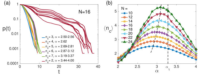
Figure 5: a) Distribution of transient times $p(t)$ for a $3$-SAT instance with $N=16$ variables and increasing number of constraints. Long chaotic transients appear when the number of solution clusters $n_{c}$ suddenly decreases (see legend). b) The average number of solution clusters $\langle n_{c}\rangle$ as function of $\alpha$ measured on $10,000$ 3-SAT instances with different number of variables $N$. The dashed line connecting the maximum of curves shifts to the right as $N$ increases, slowly converging to $\alpha_{\chi}$.

As mentioned above, the search dynamics moves in the $\bm{s}\in{\cal H}_{N}$ hypercube and solution clusters correspond to attractors, which are most of the time not single points but whole subspaces in which every point has potential energy $V=0$. In the absence of chaos the trajectory directly flows into an attractor on a path shorter than the diagonal of the hypercube $2\sqrt{N}$, so this length and consequently the characteristic time for finding the solution $\tau$ should scale with an exponent smaller than $0.5$ (the dynamics is accelerated on average due to (2)). When trajectories become longer than the diagonal, the scaling factor of the length and also of the time spent along these trajectories is larger than $0.5$, which indicates the appearance of more complicated trajectories. Therefore, it is expected that the order-chaos phase transition appears at $\eta_{c}=0.5$. Accordingly, for infinite size formulas (in the thermodynamic limit) the probability of a formula generating chaotic dynamics for our CTDS goes to zero for $\alpha<\alpha_{\chi}$ and to unity for $\alpha>\alpha_{\chi}$.

If this transition indeed corresponds to the appearance of chaos, then taking any large random formula and gradually increasing $\alpha$ by adding new constraints, chaotic dynamics should appear close to the threshold. In Figs 4(a,b) we plot a basin map for a large random instance with $N=1000$ variables at constraint density $\alpha=3.25$. Even though the basins have complicated structures, they have piecewise smooth boundaries, revealed upon subsequent magnifications. Figs 4(c,d,e) show a similar case but for a random formula obtained after adding new constraints to the existing ones such as to reach $\alpha=3.30>\alpha_{\chi}$. One can notice the fractal basin boundaries: upon subsequent magnifications the images just show more of the fractal patterns. Fig 4(f) shows the time needed to find a solution from every grid-point. Darker blue corresponds to more time taken by the trajectory. Note that a solution is identified from the orthant which the trajectory enters; as explained in Section II, one can immediately check for the solution as soon as the trajectory enters a new orthant, since checking is fast, linear-time cost. In Fig 4 we are coloring initial points by the solutions, not by the clusters, the cluster basin boundary plots have fewer colors, however, they share same behavior as the solution boundary plots, see Fig. 2 in Ref Ercsey-Ravasz and Toroczkai (2011).

V Metastable energy basins as chaos generators

Since the attractors of the CTDS correspond to solution clusters, the appearance of chaos has to be related to the structure of the solution space. At small $\alpha$ values there are many solutions grouped in only one large solution cluster and possibly a number of small ones. Detecting all of them is computationally costly, it is only possible for small SAT instances ($N\leq 24$). Taking a few formulas with $N=16$ variables and increasing $\alpha$ we monitored how the number and size of solution clusters is related to the dynamical behavior of the CTDS. We find that having a large number of solution clusters is not a sufficient condition for chaotic dynamics. Instead, it seems that chaos appears when solution clusters start to disappear (Fig.5) and metastable (non-solution) energy basins appear. A metastable or non-solution energy basin is one from which the trajectory can only escape by increasing its energy (computed as $E=\sum_{m}K_{m}^{2}$), but there is no solution in it (no point with $E=0$ inside the basin). In the energy landscape this would correspond to having deep energy valleys without solutions at their bottom; these act as temporary traps from where the dynamics will take time to escape. Fig 5(a) shows the fraction of trajectories $p(t)$ that have not yet found a solution by time $t$, for a formula with $N=16$, but increasing constraint density. The constraint density was increased by adding random clauses to the existing ones. For every case (curve) we measured the number of solution clusters $n_{c}$. One can see that as long as the number of solution clusters kept increasing the $p(t)$ curves dropped fast. However, as soon as the number of clusters decreased suddenly from 7 to 2, long transients appeared and the decay of $p(t)$ has slowed. The following gives a simple scenario by which a solution cluster disappears, but remains as a metastable basin. Consider a cluster that has three frozen spin variables (see end of Section II for the definition of a frozen variable), for example the first three: $s_{1}=1$, $s_{2}=1$ and $s_{3}=1$. Adding the new clause $\overline{x}_{1}\vee\overline{x}_{2}\vee\overline{x}_{3}$, it will make all the previous solutions in this cluster non-solutions for the new formula that includes the added clause. This addition “lifts” up uniformly by unity the energy of all the points in the cluster, thus preserving the energy distribution within the cluster and hence its basin character. When the trajectory gets trapped in this metastable cluster, it will take time to exit, after some of the auxiliary variables have sufficiently increased.

We then measured the average number of solution clusters in $10^{4}$ SAT formulas for $N\in[10,24]$ as function of $\alpha$, with the results shown in Fig 5(b). We can see that the $\alpha^{\prime}$ where the average $\langle\eta_{c}\rangle$ reaches its maximum is around $3$, but slowly shifts towards larger values with increasing $N$ (see also Ardelius and Zdeborova (2008)). A similar behavior was reported in Wang (2004) using an image computation method. The presented arguments suggest that $\alpha^{\prime}$ will converge towards $\alpha_{\chi}$ for large $N$.

VI Chaotic transition for 4-SAT

Although $k$-SAT is NP-complete for $k\geq 3$, there are studies arguing that there are qualitative differences between the hardness of $3$-SAT and $4$-SAT Montanari et al. (2008) caused by the properties of the solution space. There are heuristic algorithms which efficiently solve some of the $3$-SAT problems even from the frozen region, but they work less well for $k\geq 4$ Marino et al. (2015). For this reason we performed a similar analysis on the random $4$-SAT ensemble. We observe the same type of chaotic transition, in this case around $\alpha_{\chi}\simeq 7.85$, well below the satisfiability threshold at $\alpha_{s}=9.931$. Simulations are more costly, so we calculated the escape rate $\kappa$ and hardness $\eta$ for $J=200$ problems of size $N=50,70,100,150$ and $\alpha\in[6.0,8.4]$. The number of initial conditions used in each problem for calculating the escape rate was $5000$. In Fig.6(a) we show the distribution $P(\eta)$ at different $\alpha$ values for $N=150$. This figure is very similar to Figs.2(a),(b),(c) obtained for $3$-SAT: around a critical $\alpha$ the distributions become wider with their mean value being again around $\eta_{c}=0.5$. In Fig.6(b) the curves showing the fraction $\rho$ of problems with hardness larger than $\eta_{c}=0.5$ indicate a phase transition somewhere in the region $\alpha_{\chi}\in[7.80,7.90]$. Although the simulations are costly and the statistics is not as good as for $3$-SAT, to check if the critical value is indeed in this region, we studied a large random $4$-SAT instance with $N=1000$ variables. Adding more and more constraints, if $N$ is large enough, chaos should appear around the critical value of $\alpha_{\chi}$, as also seen for $3$-SAT in Fig.4. Indeed, figures 6(c,d) show that the basins of attraction have smooth boundaries at $\alpha=7.80$, but show fractal like features at $7.90$, indicating the appearance of chaos. The 4-SAT example shows that since our algorithm is not dependent on the specificities of the clauses, it can be used to study any SAT problem, even of mixed-type: indeed, Sudoku studied in Ercsey-Ravasz and Toroczkai (2012) is a mixed $k$-SAT problem with $k\leq 9$.

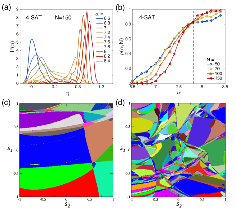
Figure 6: a) Normalized densities $P(\eta)$ of hardness for different $\alpha$ values for random satisfiable $4$-SAT instances with $N=150$ variables. b) The fraction of problems $\rho$ with $\eta>\eta_{c}=0.5$ as function of $\alpha$. Projections of basins of attraction of solutions for a large random $4$-SAT formula with $N=1000$ variables at c) $\alpha=7.80$ and d) $\alpha=7.90$.

VII No chaotic transition for 2-SAT

Next we studied the same statistics, however, for random 2-SAT ensembles. 2-SAT is in $P$ that is, there are polynomial-time algorithms that find its solutions or show that there aren’t any. The distributions of hardness measures for $N=200,1000$ are shown in Fig.7(a,b) and the average hardness $\langle\eta\rangle$ is plotted as function of $\alpha$ for different values of $N$ in Fig.7(c). We see the naturally expected increase in hardness with increasing $\alpha$, however, the transition is missing. The $\langle\eta\rangle$ curves as function of $\alpha$ do not intersect each other, the hardness increases with $N$ but rapidly saturates (there is only a very small difference between curves for $N=1000$ and 2000) and stay well below the value $\eta_{c}=0.5$. Recall that going beyond $\eta_{c}=0.5$ signals the fact that the trajectories are much longer than the typical direct distance between two points in the hypercube ${\cal H}_{N}$; this does not happen here, statistically. However, there can be specific 2-SAT problems for small $N$ for which their hardness goes a little beyond $0.5$ as seen from the tails of $P(\eta)$ in Figs 7(a,b) for large $\alpha$. We note that the satisfiability threshold is at $\alpha_{s}=1$ in 2-SAT, so for $\alpha$ values within the SAT region only the very tail of the distributions and for smaller $N$ reach barely above $\eta_{c}=0.5$. Just as in the case of 3-SAT, however, with increasing $N$, the $P(\eta)$ distributions become sharper, and thus the probability that we select randomly a formula with $\eta>0.5$ within the SAT region goes to zero. When plotting the number of solution clusters (for satisfiable instances) as function of $\alpha$, as shown in Fig 7(d) we see that for larger $N$ it is only increasing within the SAT (satisfiable) region, then it saturates afterwards.

Thus chaos disappears in the thermodynamic limit in the SAT region. Of course for unsatisfiable formulas the dynamics will be permanently chaotic, so the SAT/UNSAT transition point $\alpha_{s}$ in this case coincides with the chaotic transition point $\alpha_{\chi}$.

VIII Summary and discussion

We have shown that the escape rate, a dynamic invariant of transient chaos exhibited by the deterministic analog solver provides a suitable measure of formula hardness for individual formulas. It is sensitive to changes in the solution space, however, unlike hardness measures that are based on solution times, does not require the actual solution of the formula: it is a statistical measure describing the rate of the decay of the number of trajectories that can be estimated from within a domain in the phase space.

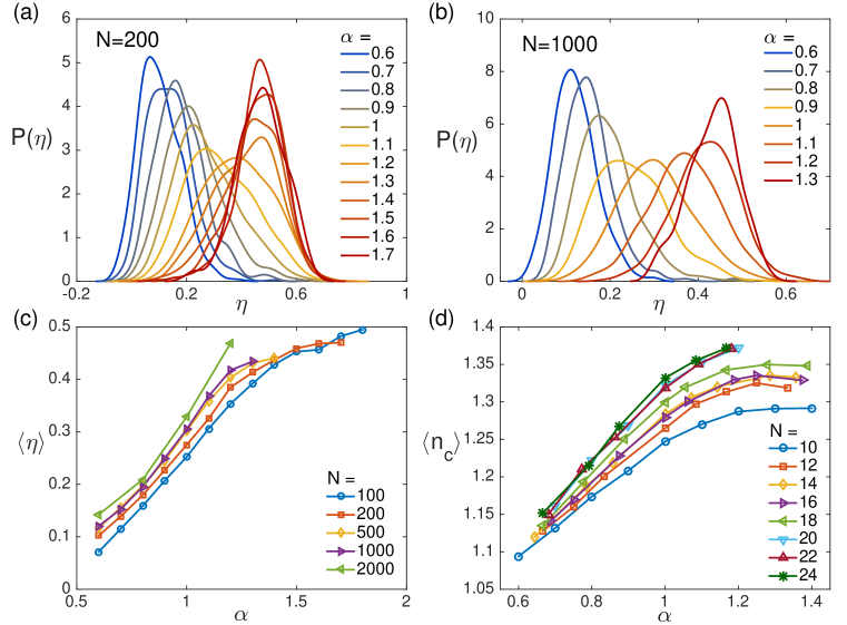
Figure 7: Normalized distribution $P(\eta)$ of hardness measures of random satisfiable $2$-SAT instances with different values of $\alpha$ (see legend) and a) $N=200$, b) $N=1000$. c) The average hardness $\langle\eta\rangle>$ and d) average number of solution clusters $\langle n_{c}\rangle$ as function of $\alpha$ for several values of $N$ (see legends).

We have provided further numerical evidence that the typical time $\tau\sim\kappa^{-1}$ needed by the analog solver to find a solution for a 3-SAT formula at a given constraint density $\alpha$ scales polynomially with the number of variables $N$:

$$\tau\sim N^{\eta}$$ (12)

where the exponent $\eta$ depends on both $\alpha$ and $N$, but in a way that it stays bounded, $\eta\in(0,\eta_{max}]$, where it was found in Ercsey-Ravasz and Toroczkai (2011) that $\eta_{max}\simeq 1.6$. It is important to mention that while the scaling (12) indicates that the solver finds solutions in polynomial analog time (not just on average but also worst case, see Ercsey-Ravasz and Toroczkai (2011)), this is done at the cost of exponential fluctuations in energy (due to the exponentially grown auxiliary variables), as shown in Ercsey-Ravasz and Toroczkai (2011), adding further numerical support to the conjecture that $P\neq NP$. The advantage of this analog approach is in possible non-Turing, special purpose physical implementations because it provides a way to trade search time for energy; while we do not have the ability to generate time, we do know how to generate energy, at least to within reasonable bounds.

We have shown that constraint satisfaction hardness appears in the form of transiently chaotic search trajectories by the deterministic CTDS. Transient chaos appears through a second-order phase transition within the random 3-SAT ensemble of formulas at a critical $\alpha_{\chi}\simeq 3.28$ such that almost no formulas have chaotic trajectories below $\alpha_{\chi}$ and almost all formulas have chaotic trajectories above $\alpha_{\chi}$, in the thermodynamic limit.

We have also shown, that surprisingly, for a given finite $N$ and at a fixed $\alpha$ the hardness distribution is Gaussian-like, which implies that the escape rate and thus the typical search time $\tau$ obeys a lognormal-like distribution indicating that within random formula ensembles there is a wide range of hardness variability (we checked for $\alpha$ over the whole range up to $\alpha_{s}$), somewhat questioning the usefulness of the random ensemble approach for finite problems. However, (10) shows that in the thermodynamic limit these distributions approach delta functions.

The typical hardness value of a formula around the critical point can be expressed from (11) as $\eta=0.5-B_{l}(\alpha_{\chi}-\alpha)^{1-\gamma}$ for $\alpha<\alpha_{\chi}$ and $\eta=0.5+B_{r}(\alpha-\alpha_{\chi})^{1-\gamma}$ for $\alpha>\alpha_{\chi}$. This implies that the escape rate for fixed $N$ has an exponential-algebraic dependence on the constraint density:

$$\kappa=\left\{\begin{array}[]{ll}\frac{1}{\sqrt{N}}e^{(B_{l}\log N)(\alpha_{\chi}-\alpha)^{1-\gamma}}\;,&\alpha<\alpha_{\chi}\\ \\ \frac{1}{\sqrt{N}}e^{-(B_{r}\log N)(\alpha-\alpha_{\chi})^{1-\gamma}}\;,&\alpha>\alpha_{\chi}\end{array}\right.$$ (16)

which is a form similar to what has been found in the theory of superpersistent chaotic transients, see Ref Lai and Tél (2011), pg 298, with the exception that for superpersistent transients the exponent $1-\gamma$ is negative and thus $\kappa$ approaches zero at the critical point, whereas here it goes through a non-zero value with a jump in its derivative at the critical point.

At this point to clarify some of the relationships between problem structure, algorithms and computational complexity. The notion of hardness refers to both the algorithm and the problem, the two cannot be separated in this context. Some problems may appear easy for some algorithms and hard for some others. This is why we connected the observed behaviors and the phase transition to the properties of the solution space. Also note that the existence and the properties of these phase transitions depend on the ensemble of formulas selected. For example, random $k$-XORSAT has a different phase diagram than random $k$-SAT, even though any $k$-XORSAT formula can be brought into a CNF SAT form (in particular, in the case of $3$-XORSAT we use four CNF 3-SAT clauses to represent one parity check equation). Note that in $k$-XORSAT the constraint density $\gamma$ is measured as the ratio between the number of parity-check equations to the number of variables. The relationship between variables and constraints can be represented as a hypergraph with nodes representing the boolean variables and hyperedges representing the parity check equations (constraints) connecting the corresponding variables (nodes) present in them. Using this representation, Mézard, Ricci-Tershengi and Zecchina have proven Mézard et al. (2003) that there is a dynamical transition point at $\gamma_{d}=0.8185$ when the statistical weights of the hyperloops (of arbitrary size) in this hypergraph becomes non-zero in the thermodynamic limit. In the Supplementary Information section of Ref Ercsey-Ravasz and Toroczkai (2011) we have shown that the corresponding chaotic transition point $\gamma_{\chi}$ for $3$-XORSAT coincides with the dynamical transition point $\gamma_{d}$ as it is at this point where chaos appears due to the appearance of small hyperloop motifs in the hypergraph. When (even small) hyperloops are present, mutual coupling appears between our equations (1), (2), and this typically leads to chaotic behavior, see Supplementary Information Sect G and Fig S4 in Ercsey-Ravasz and Toroczkai (2011). A classic example which illustrates that mutual coupling between nonlinear equations induces chaos is the Lorenz system Ott (2002).

It is also important to mention that in spite of an enormous initial excitement, the phase transition picture does not directly speak to the true nature of the algorithmic barrier $P\neq NP$. For example, even though 2-SAT is in $P$, it does have a phase transition (SAT/UNSAT transition) at constraint density $\alpha=1$ Chvátal and Reed (1992); Goerdt (1992). While $k$-XORSAT can be solved in polynomial time by Gaussian elimination (it is equivalent to a linear set of equations modulo 2) and thus it is in $P$, it presents phase transitions including the clustering transition and the SAT/UNSAT transition. Additionally, we observe the chaotic phase transition in the XORSAT as well. Moreover, HornSAT, which is solvable in linear time (thus it is also in $P$) Beeri and Bernstein (1979); Dowling and Gallier (1984), was mathematically proven Moore et al. (2005) to also present several phase transitions. The phase transition picture appears too coarse in describing the essential nature of the algorithmic barrier; one needs tools that can attack this question at the level of single formulas. The escape rate $\kappa$ or the corresponding hardness measure $\eta$ is a dynamical invariant measure of any individual SAT formula. As the nature of the dynamics (of the transient chaos) changes significantly from one hard formula to another this measure provides us with a sufficiently sensitive tool to study formula hardness as function of the matrix $C=\{c_{mi}\}$. It also opens a door to a dynamical systems approach to the $P$ vs $NP$ question.

Finally, note that system (1)-(2) is not unique; it is quite possible that there are other forms of dynamical systems that ensure that the trajectory does not get stuck in any non-solution attractors and are perhaps, even better suited for physical device implementations than these equations. Eqs (1)-(2) were introduced to be as transparent as possible, while having the necessary properties required by a deterministic analog SAT solver. However, since the chaotic transition discussed here is a property of the solution-space, on expects that other deterministic versions of the solver would also experience the same transition.

References

- Cook (1971) S.A. Cook, “The complexity of theorem-proving procedures,” in Proceedings of the Third Annual ACM Symposium on Theory of Computing (ACM, 1971) p. 151.
- Garey and Johnson (1979) M.R. Garey and D.S. Johnson, Computers and Intractability: A Guide to the Theory of NP-Completeness (Series of Books in the Mathematical Sciences), first edition ed. (W. H. Freeman & Co Ltd, 1979).
- (3) “P vs. NP and the computational complexity zoo,” https://youtu.be/YX40hbAHx3s, published on Aug 26, 2014.
- Fortnow (2009) L. Fortnow, “The status of the P versus NP problem,” Commun. ACM 52, 78 (2009).
- Ercsey-Ravasz and Toroczkai (2011) M. Ercsey-Ravasz and Z. Toroczkai, “Optimization hardness as transient chaos in an analog approach to constraint satisfaction,” Nature Physics 7, 966 (2011).
- Elser et al. (2007) V. Elser, I. Rankenburg, and Thibault P., “Searching with iterated maps,” Proceedings of the National Academy of Sciences, USA 104, 418–423 (2007).
- Hu et al. (2012a) DD. Hu, P. Ronhovde, and N. Zohar, “Phase transitions in random potts systems and the community detection problem: spin-glass type and dynamic perspectives,” Philosophical Magazine 92, 406–445 (2012a).
- Hu et al. (2012b) DD. Hu, P. Ronhovde, and N. Zohar, “Stability-to-instability transition in the structure of large-scale networks,” Physical Review E 86, 066106 (2012b).
- Ercsey-Ravasz and Toroczkai (2012) M. Ercsey-Ravasz and Z. Toroczkai, “The chaos within Sudoku,” Scientific Reports 2, 725 (2012).
- Tél and Lai (2008) T. Tél and Y.-C. Lai, “Chaotic transients in spatially extended systems,” Physics Reports 460, 245 (2008).
- Lai and Tél (2011) Y.-C. Lai and T. Tél, Transient Chaos: Complex Dynamics on Finite-Time Scales (Springer, 2011).
- Gorman et al. (1984) M. Gorman, P. J. Widmann, and K. A. Robbins, “Chaotic flow regimes in a convection loop,” Phys. Rev. Lett. 52, 2241 (1984).
- Sommerer et al. (1996) J.C. Sommerer, H.-C. Ku, and H.E. Gilreath, “Experimental evidence for chaotic scattering in a fluid wake,” Phys. Rev. Lett. 77, 5055 (1996).
- Peixinho and Mullin (2006) J. Peixinho and T. Mullin, “Decay of turbulence in pipe flow,” Phys. Rev. Lett. 96, 094501 (2006).
- Hof et al. (2006) B. Hof, J. Westerweel, T.M. Schneider, and B. Eckhardt, “Finite lifetime of turbulence in shear flows,” Nature 443, 59 (2006).
- Schwefel et al. (2004) H.G.L. Schwefel, N.B. Rex, H.E. Tureci, R.K. Chang, A.D. Stone, T. Ben-Messaoud, and J. Zyss, “Dramatic shape sensitivity of directional emission patterns from similarly deformed cylindrical polymer lasers,” J. Opt. Soc. Am. B 21, 923 (2004).
- Altmann (2009) E.G. Altmann, “Emission from dielectric cavities in terms of invariant sets of the chaotic ray dynamics,” Phys. Rev. A 79, 013830 (2009).
- Doron et al. (1990) E. Doron, U. Smilansky, and A. Frenkel, “Experimental demonstration of chaotic scattering of microwaves,” Phys. Rev. Lett. 65, 3072 (1990).
- Heagy et al. (1994) J.F. Heagy, T.L. Carroll, and L.M. Pecora, “Experimental and numerical evidence for riddled basins in coupled chaotic systems,” Phys. Rev. Lett. 73, 3528 (1994).
- de Paula et al. (2006) A.S. de Paula, M.A. Savi, and F.H.I. Pereira-Pinto, “Chaos and transient chaos in an experimental nonlinear pendulum,” J. Sound and Vibration 294, 585 (2006).
- In et al. (1998) V. In, M.L. Spano, and M. Ding, “Maintaining chaos in high dimensions,” Phys. Rev. Lett. 80, 700 (1998).
- Jánosi et al. (1994) I.M. Jánosi, L. Flepp, and T. Tél, “Exploring transient chaos in an NMR-laser experiment,” Phys. Rev. Lett. 73, 529 (1994).
- Scott et al. (1991) S.K. Scott, B. Peng, A.S. Tomlin, and K. Showalter, “Transient chaos in a closed chemical system,” J. Chem. Phys. 94, 1134 (1991).
- J.Wang et al. (1994) J.Wang, P. G. Soerensen, and F. Hynne, “Transient period doublings, torus oscillations, and chaos in a closed chemical system,” J. Phys. Chem. 98, 725 (1994).
- Motter et al. (2013) A.E. Motter, M. Gruiz, Gy. Károlyi, and T. Tél, “Doubly transient chaos: Generic form of chaos in autonomous dissipative systems,” Phys. Rev. Lett. 111, 194101 (2013).
- Kadanoff and Tang (1984a) L. P. Kadanoff and C. Tang, “Escape from strange repellers,” PNAS 81, 1276 (1984a).
- Cvitanović et al. (2009) P. Cvitanović, R. Artuso, R. Mainieri, G. Tanner, and G. Vattay, Chaos: Classical and Quantum (Niels Bohr Institute, Copenhagen, 2009).
- Kadanoff and Tang (1984b) L.P. Kadanoff and C. Tang, “Escape rate from strange repellers,” PNAS 81, 1276 (1984b).
- Kirkpatrick and Selman (1994) S. Kirkpatrick and B. Selman, “Critical-behavior in the satisfiability of random boolean expressions,” Science 264, 1297 (1994).
- Monasson and Zecchina (1996) R. Monasson and R. Zecchina, “Entropy of the k-satisfiability problem,” Phys. Rev. Lett. 76, 3881 (1996).
- Mezard et al. (2002) M. Mezard, G. Parisi, and R. Zecchina, “Analytic and algorithmic solution of random satisfiability problems,” Science 297, 812 (2002).
- Achlioptas et al. (2005) D. Achlioptas, A. Naor, and Y. Peres, “Rigorous location of phase transitions in hard optimization problems,” Nature 435, 759 (2005).
- Mézard et al. (2005a) M. Mézard, M. Palassini, and O. Rivoire, “Landscape of solutions in constraint satisfaction problems,” Phys. Rev. Lett. 95, 200202 (2005a).
- Mézard et al. (2005b) M. Mézard, T. Mora, and R. Zecchina, “Clustering of solutions in the random satisfiability problem,” Phys. Rev. Lett. 94, 197205 (2005b).
- Krzakala et al. (2007) F. Krzakala, A. Montanari, F. Ricci-Tersenghi, G. Semerjian, and L. Zdeborová, “Gibbs states and the set of solutions of random constraint satisfaction problems,” PNAS 104, 10318 (2007).
- Achlioptas (2008) D. Achlioptas, “Solution clustering in random satisfiability,” Eur. Phys. J. B. 64, 395 (2008).
- Ardelius and Zdeborova (2008) J. Ardelius and L. Zdeborova, “Exhaustive enumeration unveils clustering and freezing in the random 3-satisfiability problem,” Phys. Rev. E 78, 040101 (2008).
- Zdeborová and Mézard (2008) L. Zdeborová and M. Mézard, “Constraint satisfaction problems with isolated solutions are hard,” J. Stat. Mech.: Theor. Exp. , P12004 (2008).
- Marino et al. (2015) R. Marino, G. Parisi, and F. Ricci-Tersenghi, “The backtracking survey propagation algorithm for solving random k-sat problems,” arXiv preprint arXiv:1508.05117 (2015).
- (40) “Truncated normal distribution,” http://en.wikipedia.org/wiki/Truncated_normal_distribution, accessed on Jun 3, 2015.
- Antal et al. (2004) T. Antal, M. Droz, and Z. Rácz, “Probability distribution of magnetization in the one-dimensional Ising model: Effects of boundary conditions,” J. Phys. A: Math. Gen. 37, 1465 (2004).
- Portelli et al. (2001) B. Portelli, P.C.W. Holdsworth, M. Sellitto, and Bramwell S.T., “Universal magnetic fluctuations with a field-induced length scale,” Physical Review E 64, 036111 (2001).
- Wang (2004) X. Wang, Analysis on the assignment landscape of 3-SAT problems, MSc Thesis, Rice University, Houston, TX (2004).
- Montanari et al. (2008) A. Montanari, F. Ricci-Tersenghi, and G. Semerjian, “Clusters of solutions and replica symmetry breaking in random k-satisfiability,” Journal of Statistical Mechanics: Theory and Experiment 2008, P04004 (2008).
- Mézard et al. (2003) M. Mézard, F. Ricci-Tersenghi, and R. Zecchina, “Two solutions to diluted p-spin models and xorsat problems,” Journal of Statistical Physics 111, 505 (2003).
- Ott (2002) E. Ott, Chaos in dynamical systems (Cambridge University Press, 2002).
- Chvátal and Reed (1992) V. Chvátal and B. Reed, “Mick gets some (the odds are on his side)[satisfiability],” in Foundations of Computer Science, 1992. Proceedings., 33rd Annual Symposium on (IEEE, 1992) pp. 620–627.
- Goerdt (1992) A. Goerdt, “A threshold for unsatisfiability,” in Mathematical foundations of computer science 1992 (Springer, 1992) pp. 264–274.
- Beeri and Bernstein (1979) C. Beeri and P.A. Bernstein, “Computational problems related to the design of normal form relational schemas,” ACM Trans. Database Syst. 4, 30 (1979).
- Dowling and Gallier (1984) W.F Dowling and J.H. Gallier, “Linear-time algorithms for testing the satisfiability of propositional Horn formulae,” The Journal of Logic Programming 1, 267 (1984).
- Moore et al. (2005) C. Moore, G. Istrate, D. Demopoulos, and M.Y. Vardi, “A continuous-discontinuous second-order transition in the satisfiability of random Horn-SAT formulas,” in Approximation, Randomization and Combinatorial Optimization. Algorithms and Techniques (Springer, 2005) pp. 414–425.