Occupation times of alternating renewal processes
with Lévy applications

Abstract   This paper presents a set of results relating to the occupation time $\alpha(t)$ of a process $X(\cdot)$. The first set of results concerns exact characterizations of $\alpha(t)$, e.g., in terms of its transform up to an exponentially distributed epoch. In addition we establish a central limit theorem (entailing that a centered and normalized version of $\alpha(t)/t$ converges to a zero-mean Normal random variable as $t\to\infty$) and the tail asymptotics of ${\mathbb{P}}(\alpha(t)/t\geq q)$. We apply our findings to spectrally positive Lévy processes reflected at the infimum and establish various new occupation time results for the corresponding model.

Keywords   Occupation time $\circ$ alternating renewal process $\circ$ Lévy process $\circ$ reflected Brownian motion $\circ$ central limit theorem $\circ$ large deviations

Affiliations   N. Starreveld is with Korteweg-de Vries Institute for Mathematics, Science Park 904, 1098 XH Amsterdam, University of Amsterdam, the Netherlands. Email: N.J.Starreveld@uva.nl.

R. Bekker is with Department of Mathematics, Vrije Universiteit Amsterdam, De Boelelaan 1081a, 1081 HV Amsterdam, the Netherlands. Email: r.bekker@vu.nl.

M. Mandjes is with Korteweg-de Vries Institute for Mathematics, University of Amsterdam, Science Park 904, 1098 XH Amsterdam, the Netherlands. He is also affiliated with Eurandom, Eindhoven University of Technology, Eindhoven, the Netherlands, and CWI, Amsterdam the Netherlands. Email: m.r.h.mandjes@uva.nl.

1 Introduction

In this paper we consider a stochastic process $X(\cdot)\equiv\{X(t):t\geq 0\}$ taking values on the state space $E$, and a partition of the state space $E=A\cup B$ into two (disjoint) sets $A,B$. Specifically, $X(\cdot)$ is an alternating renewal process where the sojourn times in set $B$ depend on the sojourn times in $A$. The object of study is the occupation time, denoted by $\alpha(t)$, of the set $A$ up to time $t$, defined by

$$\alpha(t)=\int_{0}^{t}1_{\{X(s)\in A\}}{\rm d}s;$$ (1.1)

as the set $A$ is held fixed, we suppress it in our notation. Such occupation measures appear naturally when studying stochastic processes, and are useful in the context of a wide variety of applications. Our primary source of motivation stems from the study of occupation times of (reflected) spectrally positive Lévy processes, where such an alternating renewal structure appears naturally.

Scope & contributions

Our results essentially cover two regimes. In the first place we present results characterizing the transient behavior of $\alpha(t)$, in terms of expressions for the transform of $\alpha(e_{q})$, with $e_{q}$ being exponentially distributed with mean $q^{-1}$. Secondly, the probabilistic properties of $\alpha(t)$ for $t$ large are captured by a central limit theorem and large deviations asymptotics. We also include a series of new results in which we specialize to the situation that $X(\cdot)$ corresponds to a spectrally positive Lévy process reflected at its infimum; for instance, we determine an explicit expression of the double transform of the occupation time $\alpha(t)$. For the case of an unreflected process, we recover a distributional relation between the occupation time of the negative half line up to an exponentially distributed amount of time, and the epoch at which the supremum is attained (over the same time interval). Our results have been recently used to study processes with two reflecting barriers [41].

Relation to existing literature

The occupation time of a stochastic process was first considered in [43], resulting in an expression for the distribution function of $\alpha(t)$ that enabled the derivation of a central limit theorem; a similar result was also established in [46] using renewal theory. In [15, 32, 33] occupation times of spectrally negative Lévy processes were studied, while in [31] refracted Lévy processes were dealt with; these results are typically occupation times until a first passage time. Occupation times up to a fixed time horizon $t$ have been studied in [24] for spectrally negative Lévy processes and in [45] for a general Lévy process which is not a compound Poisson process. The cases in which $X(\cdot)$ is a Brownian motion, or Markov-modulated Brownian motion have been extensively studied; see e.g. [10, 14, 17, 36] and references therein. A variety of results specifically applying to Brownian motion and reflected standard normal Brownian motion can be found in [13]. Occupation times of dam processes were considered in [16]. Occupation times and its application to service levels over a finite interval in multi-server queues were dealt with in [7, 40]. Applications in machine maintenance and telegraph processes can be found in [43, 46].

This paper generalizes the results established in [16, 43, 46]. The setup of [43, 46] assumes that the successive time intervals that $X(\cdot)$ spends in the two sets $A$ and $B$ form two independent sequences of i.i.d. random variables, whereas we relax this assumption; the motivation for pursuing this extension lies in the fact that in many models we observe dependency between such intervals. Our methodology also generalizes the methods of [16]: there, relying on renewal theory, specific mean quantities are found, whereas we uniquely characterize the corresponding full distributions. The results we prove can be applied to a broad class of processes including spectrally one-sided Lévy processes with or without reflecting barriers. The large deviations result we prove is an additional novelty of this paper, to the authors knowledge large deviations asymptotics for occupation times have not been studied before in the literature.

Organization

The structure of the paper is as follows. Section 2 describes the model and presents the application that motivated our research, i.e., storage models and spectrally positive Lévy processes reflected at its infimum. In Section 3 we present our main results and show how our findings can be applied to reflected spectrally positive Lévy processes. Then, in Section 4, we derive the expression for the double transform of the occupation time. Section 5 provides the proof of the central limit theorem, and Section 6 of the large deviations result. The more technical proofs are included in an appendix.

2 Model and Applications

First we provide a general model description in Section 2.1. Then we introduce the more specific class of reflected spectrally positive Lévy processes in Section 2.2, where we distinguish two cases, viz. storage models and general reflected spectrally positive Lévy processes.

2.1 Model description

We consider a stochastic process $X(\cdot)\equiv\{X(t):t\geq 0\}$ taking values on the state space $E$, and a partition of $E$ into two disjoint subsets, denoted by $A$ and $B$, i.e., $E=A\cup B$ and $A\cap B=\emptyset$. Then, $X(\cdot)$ alternates between $A$ and $B$. The successive sojourn times in $A$ are $(D_{i})_{i\in{\mathbb{N}}}$, and those in $B$ are $(U_{i})_{i\in{\mathbb{N}}}$. If $(D_{i})_{i\in{\mathbb{N}}}$ and $(U_{i})_{i\in{\mathbb{N}}}$ are independent sequences of i.i.d. random variables, the resulting process is an alternating renewal process, and has been considered in e.g. [43, 46]. In this paper, however, we consider the more general situation in which $(D_{i},U_{i})_{i\in{\mathbb{N}}}$ is a sequence of i.i.d. bivariate random vectors that are distributed according to the generic random vectors $(D,U)$, but without requiring $D$ and $U$ to be independent. In the paper we prove our results for the case $X(0)\in A$, but the case $X(0)\in B$ can be treated along the same lines; also the case that $D_{1}$ has a different distribution can be dealt with, albeit at the expense of more complicated expressions.

2.2 Spectrally positive Lévy processes

A stochastic process $X(\cdot)$ defined on a probability space $(\Omega,\mathcal{F},\operatorname{\mathbb{Pb}})$ is called a Lévy process if $X(0)=0$, it has almost surely càdlàg paths, and it has stationary and independent increments. Typical examples of Lévy processes are Brownian motion and the (compound) Poisson process. The Lévy-Khinchine representation relates Lévy processes with infinitely divisible distributions and it provides the following representation for the characteristic exponent $\Psi(\theta):=-\log\operatorname{\mathbb{E}}(e^{{\rm i}\theta X(1)})$:

$$\Psi(\theta)={\rm i}d\theta+\frac{1}{2}\sigma^{2}\theta^{2}+\int_{\mathbb{R}}(1-e^{{\rm i}\theta x}+{\rm i}\theta x1_{\{|x|<1\}})\Pi({\rm d}x),$$

where $d\in\mathbb{R}$, $\sigma^{2}>0$ and $\Pi(\cdot)$ is a measure concentrated on $\mathbb{R}\backslash\{0\}$ satisfying $\int_{\mathbb{R}}(1\wedge x^{2})\Pi({\rm d}x)<\infty$. We refer to [8, 29] for an overview of the theory of Lévy processes. When the measure $\Pi(\cdot)$ is concentrated on the positive real line then $X(\cdot)$ exhibits jumps only in the upward direction and we talk about a spectrally positive Lévy process. For a spectrally positive Lévy process $X(\cdot)$ with a negative drift, i.e. $\operatorname{\mathbb{E}}X(1)<0$, the Laplace exponent $\phi(\alpha):=\log\operatorname{\mathbb{E}}e^{-\alpha X(1)}$ is a well defined, finite, increasing and convex function for all $\alpha\geq 0$, so that the inverse function $\psi(\cdot)$ is also well defined; if it does not have a negative drift, we have to work with the right-inverse.

Given a Lévy process $X(\cdot)$ we define the process $Q(\cdot)$, commonly referred to as $X(\cdot)$ reflected at its infimum [8, 29], by $Q(t)=X(t)+L(t),$ where $L(t)$ is the regulator process (or local time at the infimum) which ensures that $Q(t)\geq 0$ for all $t\geq 0$. Hence the process $L(\cdot)$ can increase at time $t$ only when $Q(t)=0$, that is, $\int_{0}^{T}Q(t){\rm d}L(t)=0$ for all $T>0.$ This leads to a Skorokhod problem with the following solution: with $Q(0)=w$,

$$L(t)=\max\left\{w,\sup_{0\leq s\leq t}-X(s)\right\},\>\>\>\>Q(t)=X(t)+\max\left\{w,\sup_{0\leq s\leq t}-X(s)\right\}.$$

For the process $Q(t)$ and a given level $\tau\geq 0$, the occupation time of the set $[0,\tau]$ is defined by

$$\alpha(t)=\int_{0}^{t}1_{\{Q(s)\leq\tau\}}{\rm d}s.$$ (2.1)

Storage models

Storage models are used to model a reservoir that is facing supply (input) and demand (output). Supply and demand are either described by sequences of random variables $(\eta_{i})_{i\in{\mathbb{N}}}$ and $(\xi_{i})_{i\in{\mathbb{N}}}$, or by an input process $A(\cdot)$ and an output process $B(\cdot)$. Storage models can be used to control the level of stored material by regulating supply and demand. Early applications [34] of such models concern finite dams which are constructed for storage of water; see [22] for additional applications of storage models and [37, 27, 34] for a historic account of the exact mathematical formulation of the content process. We refer to [38, Ch. IV] and [29, Ch. IV] for an overview of dams and general storage models in continuous time.

A general storage model consists of a (cumulative) arrival process $A(\cdot)$ and a (cumulative) output process $B(\cdot)$, leading to the net input process $V(\cdot)$ defined by $V(t)=A(t)-B(t)$; the work stored in the system at time $t$, denoted by $Q(t)$, is defined by applying the reflection mapping, as defined above, to $V(\cdot)$. First we look into the case that $B(\cdot)$ corresponds to a positive linear trend, whereas $A(\cdot)$ is a pure jump subordinator. Thus, $V(t)=X(t)+w$ where $X(t)=A(t)-rt$ and $w=V(0)$ is the initial amount of work stored in the system. By construction, $X(\cdot)$ is a spectrally positive Lévy process; without loss of generality, we assume that $r=1$.

The reflected process $Q(\cdot)$ has an interesting path structure: it has a.s. paths of bounded variation and has only jumps in the upward direction, such that upcrossings of a level occur with a jump whereas downcrossings of a level occur with equality. Moreover, from the Lévy-Khinchine representation we have that if the Lévy measure $\Pi(\cdot)$ satisfies $\Pi((0,\infty))=\infty$, then $X(\cdot)$ exhibits countably infinite jumps in every finite interval of time. For the analysis of the occupation time $\alpha(t)$ we observe that the process $Q(\cdot)$ alternates between the two sets $A=[0,\tau]$ and $B=(\tau,\infty)$. We define the following first passage times, for $\tau\geq 0$,

$$\tau_{\alpha}=\inf_{t>0}\{t:Q(t)>\tau\,|\,Q(0)=\tau\},\>\>\>\tau_{\beta}=\inf_{t>\tau_{\alpha}}\{t:Q(t)=\tau\,|\,Q(0)=\tau\}.$$ (2.2)

Observe that $Q(\tau_{\alpha})>\tau$. In case $\operatorname{\mathbb{E}}A(1)<r$ the process keeps on having downcrossings of level $\tau$. Call the sequence of successive downcrossings $(T_{i})_{i\in{\mathbb{N}}}$. As shown in [16, Thms. 1 and 2] relying on the bounded variation property of the paths, $(T_{i})_{i\in{\mathbb{N}}}$ is a renewal process, and hence $(D_{i})_{i\in{\mathbb{N}}}$ and $(U_{i})_{i\in{\mathbb{N}}}$ are sequences of well defined random variables. In addition, $(D_{i+1},U_{i+1})$ is independent of $(D_{1},U_{1},D_{2},U_{2},\ldots,D_{i},U_{i})$; at the same time the overshoot (over level $\tau$) makes $D_{i}$ and $U_{i}$ dependent. In Fig. 1 an illustrative realization of $Q(\cdot)$ is depicted for the case of finitely many jumps in a bounded time interval.

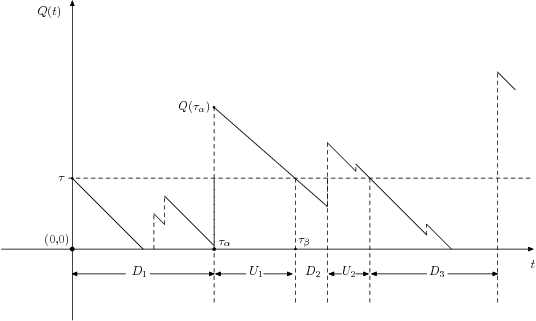
Figure 1: Sample path for the case of finitely many jumps in a bounded interval of time.

General spectrally positive Lévy processes

When the process $X(\cdot)$ is an arbitrary spectrally positive Lévy process (i.e., we deviate from the setting of $A(\cdot)$ being a pure jump process and $B(\cdot)$ a positive linear trend), then $Q(\cdot)$ may have a more complicated path structure. We may have paths of unbounded variation, and as a result the intervals $D_{i}$ and $U_{i}$ are not necessarily well defined. But even in this case it is still possible, as will be shown in Section 3.5, to study the occupation time of $[0,\tau]$ for the reflected process $Q(\cdot)$, and also the occupation time of $(-\infty,0)$ for the free process $X(\cdot)$. This is done relying on an approximation procedure: we first approximate a general spectrally positive Lévy process by a process with paths of bounded variation, and then use a continuity argument to show that the results for the bounded variation case carry over to the general spectrally positive case.

In line with Section 2.1, we prove the results for the case the process starts at $\tau$. Having a different initial position requires a different distribution of $(D_{1},U_{1})$. This case can be treated along the same lines leading to more extensive notation and expressions and is therefore omitted.

3 Overview of results

In this section we present the main results of the paper. As pointed out in the introduction, they cover two regimes.

• In the first place we present results characterizing the transient behavior of $\alpha(t)$. We identify an expression for the distribution function of $\alpha(t)$; the proof resembles that was developed in [43, Thm. 1] for the alternating renewal case. The expressions for the transform of $\alpha(e_{q})$, with $e_{q}$ exponentially distributed with mean $q^{-1}$, are found by arguments similar to those used in [12], but taking into account the dependence between $D$ and $U$. The resulting double transform is a new result, which also covers the alternating renewal case with independent $D$ and $U$, as was considered in [43], and is in terms of the joint transform of $D$ and $U$. In Section 3.5 we specify this joint transform for the models of Section 2.2.

• For the asymptotic behavior of $\alpha(t)$ we prove a central limit theorem and large deviations asymptotic. The central limit result generalizes [43, Theorem 2], that covers the alternating renewal case. The result features the quantity $c={\rm Cov}(D,U)$; in Section 3.5 we identify closed-form expressions for $c$ for the models described in Section 2.2. The large deviations principle is proven by using the Gärtner-Ellis theorem [19].

3.1 Distribution of $\alpha(t)$

We assume $(D_{i},U_{i})_{i\in{\mathbb{N}}}$ to be sequences of i.i.d. random vectors, distributed as the generic random vector $(D,U)$; $D$ and $U$ have distribution functions $F(\cdot)$ and $G(\cdot)$, respectively. We define $X_{n}=D_{1}+\ldots+D_{n}$ and $Y_{n}=U_{1}+\ldots+U_{n}$. In addition to $\alpha(t)$, we define the occupation time of $B$ by

$$\beta(t)=\int_{0}^{t}1_{\{X(s)\in B\}}{\rm d}s=t-\alpha(t).$$ (3.1)

The proof of the following result is analogous to that of [43, Thm. 1].

Proposition 3.1.

For $X(0)\in A$ and $0\leq x<t$,

$$\operatorname{\mathbb{Pb}}(\alpha(t)<x) = F(x)-\sum_{n=1}^{\infty}\big{[}\operatorname{\mathbb{Pb}}(Y_{n}\leq t-x,X_{n}<x)-\operatorname{\mathbb{Pb}}(Y_{n}\leq t-x,X_{n+1}<x)\big{]},$$ (3.2)

$$\operatorname{\mathbb{Pb}}(\beta(t)\leq x) = \sum_{n=0}^{\infty}\big{[}\operatorname{\mathbb{Pb}}(Y_{n}\leq x,X_{n}<t-x)-\operatorname{\mathbb{Pb}}(Y_{n}\leq x,X_{n+1}<t-x)\big{]}.$$ (3.3)

Remark 1.

If $X(0)\in A$, then $\beta(t)$ has an atom at 0; the mass at 0 is given by $\operatorname{\mathbb{Pb}}(\beta(t)=0)=1-F(t)$. Similarly, if $X(0)\in B$, then $\alpha(t)$ has an atom at 0; the mass at 0 equals $\operatorname{\mathbb{Pb}}(\alpha(t)=0)=1-G(t)$.

Remark 2.

If $D_{i}$ and $U_{i}$ are independent random variables, then (3.3) takes the simpler form

$$\operatorname{\mathbb{Pb}}(\beta(t)\leq x)=\sum_{n=0}^{\infty}G^{(n)}(x)\big{[}F^{(n)}(t-x)-F^{(n+1)}(t-x)\big{]},$$

where $F^{(n)}(\cdot)$ and $G^{(n)}(\cdot)$ are the $n$-fold convolutions of the distribution functions $F(\cdot)$ and $G(\cdot)$ with itself, respectively.

3.2 Transform of $\alpha(t)$

From Proposition 3.1 we observe that the distribution function of $\alpha(t)$ is rather complicated to work with. In this section we therefore focus on

$$\int_{0}^{\infty}e^{-qt}\operatorname{\mathbb{E}}e^{-\theta\alpha(t)}{\rm d}t=\frac{1}{q}\operatorname{\mathbb{E}}e^{-\theta\alpha(e_{q})},$$ (3.4)

where $e_{q}$ is an exponentially distributed random variable with mean $q^{-1}$; using a numerical inversion algorithm [1, 2, 5, 20], one can then obtain an accurate approximation for the distribution function of $\alpha(t)$. The method we use to determine the transform in (3.4) relies on the following line of reasoning: (i) we start an exponential clock at time 0, (ii) knowing that $X(0)\in A$, we distinguish between $X(\cdot)$ still being in $A$ at $e_{q}$, or $X(\cdot)$ having left $A$ at $e_{q}$, (iii) in the latter case we distinguish between $X(\cdot)$ being still in $B$ at $e_{q}$, or $X(\cdot)$ having left $B$. Using the memoryless property of the exponential distribution and the independence of $D_{i+1}$ and $U_{i}$ we can then sample the exponential distribution again, and this procedure continues until the exponential clock expires. Let

$$L_{1}(\theta)=\operatorname{\mathbb{E}}e^{-\theta D}\hskip 5.69054pt\text{and}\hskip 5.69054ptL_{1,2}(\theta_{1},\theta_{2})=\operatorname{\mathbb{E}}e^{-\theta_{1}D-\theta_{2}U}.$$ (3.5)

The main result concerning the transform of the occupation time $\alpha(t)$ is given below.

Theorem 3.1.

For the transform of the occupation time $\alpha(t)$ we have

$$\int_{0}^{\infty}e^{-qt}\operatorname{\mathbb{E}}e^{-\theta\alpha(t)}{\rm d}t=\frac{1}{1-L_{1,2}(q+\theta,q)}\left[\frac{1-L_{1}(q+\theta)}{q+\theta}+\frac{L_{1}(q+\theta)-L_{1,2}(q+\theta,q)}{q}\right].$$ (3.6)

Remark 3.

Theorem 3.1 shows that the transform of the random variable $D$ and the joint transform of $D,U$ are needed in order to compute the transform of $\alpha(t)$. These quantities are model specific, i.e., we have to assume $X(\cdot)$ has some specific structure to be able to compute them. In Section 3.5 we come back to this issue, and we compute these quantities for the models considered in Section 2.2.

Availability function

Another performance measure that is used in many applications, particularly in the theory of machine maintenance scheduling and reliability, see e.g. [46], is the availability function $\operatorname{\mathbb{Pb}}(X(\cdot)\in A\,|\,X(0)\in A)$, of which the transform is given in the following proposition.

Proposition 3.2.

For $q\geq 0$, with $L_{1}(\cdot)$ and $L_{1,2}(\cdot,\cdot)$ given in $(\ref{transforms 12})$,

$$\int_{0}^{\infty}e^{-qt}\operatorname{\mathbb{Pb}}(X(t)\in A|X(0)\in A){\rm d}t = \frac{1}{q}\frac{1-L_{1}(q)}{1-L_{1,2}(q,q)}$$ (3.7)

$$\int_{0}^{\infty}e^{-qt}\operatorname{\mathbb{Pb}}(X(t)\in B|X(0)\in A){\rm d}t = \frac{1}{q}\frac{L_{1}(q)-L_{1,2}(q,q)}{1-L_{1,2}(q,q)}.$$ (3.8)

3.3 Central Limit Theorem

Where Proposition 3.1 and Theorem 3.1 entail that the full joint distribution of $D$ and $U$ is essential when characterizing $\alpha(t)$, the next theorem shows that in the central limit regime only the covariance is needed. From [43] we have that, for the case $D$ and $U$ are independent, under appropriate scaling, $\alpha(t)$ and $\beta(t)$ are asymptotically normally distributed; our result shows that the asymptotic normality carries over to our model, with an adaptation of the parameters to account for the dependence between $D$ and $U$. We write $\alpha=\operatorname{\mathbb{E}}D$, $\beta=\operatorname{\mathbb{E}}U,$ $\sigma_{\alpha}^{2}=\operatorname{Var}D$, $\sigma_{\beta}^{2}=\operatorname{Var}U$, and $c={\rm Cov}(D,U).$ We rule out the case of perfect correlation, i.e., we assume that $c<\sigma_{\alpha}\sigma_{\beta}$.

Theorem 3.2.

Assuming $\sigma_{\alpha}^{2}+\sigma_{\beta}^{2}<\infty$, with $\Phi(\cdot)$ the standard Normal distribution function,

$$\lim_{t\rightarrow\infty}\operatorname{\mathbb{Pb}}\left(\frac{\alpha(t)-\frac{\alpha t}{\alpha+\beta}}{\sqrt{\frac{\beta^{2}\sigma_{\alpha}^{2}+\alpha^{2}\sigma_{\beta}^{2}-2\alpha\beta c}{(\alpha+\beta)^{3}}t}}<x\right)=\Phi(x)\hskip 5.69054pt\text{and}\hskip 5.69054pt\lim_{t\rightarrow\infty}\operatorname{\mathbb{Pb}}\left(\frac{\beta(t)-\frac{\beta t}{\alpha+\beta}}{\sqrt{\frac{\beta^{2}\sigma_{\alpha}^{2}+\alpha^{2}\sigma_{\beta}^{2}-2\alpha\beta c}{(\alpha+\beta)^{3}}t}}\leq x\right)=\Phi(x)$$ (3.9)

Remark 4.

In Section 3.5 we compute $\alpha$, $\beta$, $\sigma_{\alpha}^{2},\sigma_{\beta}^{2}$, and $c$ for the models introduced in Section 2.2.

3.4 Large Deviations Result

Where Thm. 3.2 concerns the behaviour of $\alpha(t)/t$ and $\beta(t)/t$ around their respective means, we now focus on their tail behavior. To this end, we study $\operatorname{\mathbb{Pb}}(\alpha(t)/t>q)$ for $t$ large, with $q>{\alpha}/({\alpha+\beta})$. Our result makes use of the following objects:

$$\lambda(\theta)=\lim_{t\rightarrow\infty}\frac{1}{t}\log\operatorname{\mathbb{E}}e^{\theta\alpha(t)},\>\>\>\>\lambda^{*}(q)=\sup_{\theta\in\mathbb{R}}\big{(}\theta q-\lambda(\theta)\big{)},$$

usually referred to as the cumulant generating function and its Legendre-Fenchel transform, respectively. The following result shows that the large deviations of $\alpha(t)/t$ require the joint transform of $D$ and $U$ being available. It requires that the moment generating function ${\mathbb{E}}\,e^{\theta D}$ is finite for $\theta$ in a neighborhood of the origin.

Theorem 3.3.

Assuming $\alpha,\beta<\infty$, if the cumulant generating function $\lambda(\theta)$ exists as an extended real number, then,

$$\lim_{t\rightarrow\infty}\frac{1}{t}\log\operatorname{\mathbb{Pb}}\left(\frac{\alpha(t)}{t}>q\right)=-\lambda^{*}(q),$$ (3.10)

for any $q>{\alpha}/({\alpha+\beta})$. The cumulant generating function $\lambda(\theta)$ equals $\theta d(\theta)$, where for a given $\theta$, $d(\theta)$ solves

$$\operatorname{\mathbb{E}}e^{\theta(1-d(\theta))\,D\,-\,\theta\,d(\theta)\,U}=1.$$ (3.11)

3.5 Spectrally positive Lévy processes

In this section we compute the quantities needed in Thms. 3.1, 3.2 and 3.3 for the models introduced in Section 2.2., with a focus on spectrally-positive Lévy processes with negative drift. Before presenting the main analysis we recall some results on scale functions that we need in our analysis [29].

Scale functions

When studying spectrally one-sided Lévy processes results are often expressed in terms of so-called scale functions, denoted by $W^{(q)}(\cdot)$ and $Z^{(q)}(\cdot)$, for $q\geq 0$. We will use the notation $W(\cdot),Z(\cdot)$ for the scale functions $W^{(0)}(\cdot)$ and $Z^{(0)}(\cdot)$. Given a spectrally positive Lévy process $X(\cdot)$ with Laplace exponent $\phi(\cdot)$, there exists an increasing and continuous function $W^{(q)}(\cdot)$ whose Laplace transform satisfies, for $x\geq 0$, the equation

$$\int_{0}^{\infty}e^{-\theta x}W^{(q)}(x){\rm d}x=\frac{1}{\phi(\theta)-q}\hskip 14.22636pt\text{for }\theta>\psi(q),$$

with $\psi(\cdot)$ the inverse function of $\phi(\cdot)$. For $x<0$, we define $W^{(q)}(x)=0$. In addition,

$$Z^{(q)}(x)=1+q\int_{0}^{x}W^{(q)}(y){\rm d}y.$$

In most of the literature, the theory of scale functions is developed for spectrally negative Lévy processes but similar results can be proven for spectrally positive Lévy processes. We also define, for $\theta$ such that $\phi(\theta)<\infty$ and $q\geq\phi(\theta)$, the functions

$$W_{\theta}^{(q-\phi(\theta))}(x)=e^{-\theta x}W^{(q)}(x)\hskip 14.22636pt\text{and}\hskip 14.22636ptZ_{\theta}^{(q-\phi(\theta))}(x)=1+(q-\phi(\theta))\int_{0}^{x}W_{\theta}^{(q-\phi(\theta))}(y){\rm d}y.$$ (3.12)

To formally define the functions $W_{\theta}^{(q-\phi(\theta))}(\cdot)$, $Z_{\theta}^{(q-\phi(\theta))}(\cdot)$ we need to perform an exponential change of measure; we refer to [6, 29] for further details. For the case $X(\cdot)$ is a spectrally positive (resp. spectrally negative) Lévy process the scale function $W(\cdot)$ directly relates to the distribution function of the running maximum (resp. running minimum) of $X(\cdot)$. For a more extensive account of the theory of scale functions and exit problems for Lévy processes we refer to [6, 8, 25, 28, 29].

Storage models

To apply Thms. 3.1, 3.2 and 3.3 we need the joint transform of $U$ and $D$; given this transform we can compute the transform of the occupation time using (3.6), find the covariance $c=\operatorname{Cov}(D,U)$ and the variances $\sigma_{\alpha}^{2}$, $\sigma_{\beta}^{2}$ needed in Thm. 3.2, and solve (3.11).

First we find representations for $D$ and $U$. Observe that $D$ is distributed as the time between a downcrossing of level $\tau$ and the next upcrossing of it: with $\tau_{\alpha}$ as defined in (2.2),

$$D=\tau_{\alpha}\hskip 14.22636pt\text{{\color[rgb]{0,0,0}a.s}}.$$ (3.13)

The time between an upcrossing and the next downcrossing, i.e., $U$, is essentially a first exit time starting from a random point which is sampled from the overshoot distribution. Defining $\sigma_{x}^{(+)}=\inf_{t>0}\{t:Q(t)\leq\tau\,|\,Q(0)=x\}$, we have

$$U=\tau_{\beta}-\tau_{\alpha}=\sigma_{Q(\tau_{\alpha})}^{(+)}\hskip 14.22636pt\text{{\color[rgb]{0,0,0}a.s}}.$$ (3.14)

The two distributional equalities (3.13) and (3.14) yield an expression for the covariance $c=\operatorname{Cov}(D,U)$:

$$\operatorname{Cov}(D,U)=\operatorname{\mathbb{E}}[DU]-\operatorname{\mathbb{E}}D\,\operatorname{\mathbb{E}}U=\operatorname{\mathbb{E}}\left[\tau_{\alpha}\,\sigma_{Q(\tau_{\alpha})}^{(+)}\right]-\operatorname{\mathbb{E}}D\,\operatorname{\mathbb{E}}U.$$

Proposition 3.3.

(i) The means $\alpha=\operatorname{\mathbb{E}}D$ and $\beta=\operatorname{\mathbb{E}}U$ equal

$$\operatorname{\mathbb{E}}D=\frac{W(\tau)}{W^{\prime}(\tau)},\>\>\>\operatorname{\mathbb{E}}U=\frac{1}{W^{\prime}(\tau)}\Big{(}\psi^{\prime}(0)-W(\tau)\Big{)},$$ (3.15)

(ii) The joint transform of $D$ and $U$ equals, with $p=\theta_{1}-\theta_{2}$,

$$\operatorname{\mathbb{E}}e^{-\theta_{1}D-\theta_{2}U} =\frac{W_{\psi(\theta_{2})}^{(p)\hskip 2.0pt^{\prime}}(\tau)+(\psi(\theta_{2})-p)W_{\psi(\theta_{2})}^{(p)}(\tau)-\psi(\theta_{2})Z_{\psi(\theta_{2})}^{(p)}(\tau)}{W_{\psi(\theta_{2})}^{(p)\hskip 2.0pt^{\prime}}(\tau)+\psi(\theta_{2})W_{\psi(\theta_{2})}^{(p)}(\tau)}.$$ (3.16)

(iii) The variances $\sigma_{\alpha}^{2}=\operatorname{Var}D$ and $\sigma_{\beta}^{2}=\operatorname{Var}U$ and covariance $c=\operatorname{Cov}(D,U)$ equal

$$\sigma_{\alpha}^{2} =-2\frac{(W\star W)(\tau)}{W^{\prime}(\tau)}+\frac{W(\tau)\left(2(W\star W)^{\prime}(\tau)-W(\tau)\right)}{W^{\prime}(\tau)^{2}},$$ (3.17)

$$\sigma_{\beta}^{2} =\frac{2\psi^{\prime}(0)}{W^{\prime}(\tau)}\left(\int_{0}^{\tau}W(y){\rm d}y+\frac{W(\tau)}{W^{\prime}(\tau)}\right)-\frac{1}{W^{\prime}(\tau)}\left(\psi^{\prime\prime}(0)+2\psi^{\prime}(0)^{2}\tau+\frac{\psi^{\prime}(0)}{W^{\prime}(\tau)}+\frac{W(\tau)^{2}}{W^{\prime}(\tau)}\right),$$ (3.18)

$$c =\big{(}\psi^{\prime}(0)-W(\tau)\big{)}\frac{1}{(W^{\prime}(\tau))^{2}}\left((W\star W)^{\prime}(\tau)-W(\tau)\right)+\frac{(W\star W)(\tau)}{W^{\prime}(\tau)}-\frac{\psi^{\prime}(0)}{W^{\prime}(\tau)}\int_{0}^{\tau}W(x){\rm d}x.$$ (3.19)

Remark 5.

The arguments used can be adapted to the case that $D_{1}$ has a different distribution than $D_{2},D_{3},\ldots$. The only difference is that the first cycle $D_{1},U_{1}$ has to be treated separately.

General spectrally positive Lévy process

As mentioned before, when $X(\cdot)$ is a general spectrally positive Lévy process, with possibly paths of unbounded variation, then the reasoning presented above does not apply. The following theorem, however, shows that our result for the occupation time $\alpha(t)$ carries over to this case as well.

Theorem 3.4.

Consider a spectrally positive Lévy process reflected at its infimum. With $A=[0,\tau]$ and $q,\theta\geq 0$,

$$\int_{0}^{\infty}e^{-qt}\operatorname{\mathbb{E}}e^{-\theta\alpha(t)}{\rm d}t=\frac{1}{q}\frac{\psi(q)Z_{\psi(q)}^{(\theta)}(\tau)}{\theta W_{\psi(q)}^{(\theta)}(\tau)+\psi(q)Z_{\psi(q)}^{(\theta)}(\tau)}.$$ (3.20)

Letting the initial level $\tau\rightarrow\infty$, the effect of the reflection becomes negligible and the time the reflected process spends below the initial level $\tau$ converges to time the unreflected reflected process that started in the origin spends below 0. Consequently, taking $\tau\to\infty$ in (3.20), we obtain the occupation time of the set $(-\infty,0]$ for the free process $X(\cdot)$ and recover a version of the Sparre Andersen’s identity, see e.g. [8, Lemma VI.15], [32, Remark 4.1], or [26].

Corollary 3.1.

Consider a spectrally positive Lévy process; the occupation time of $(-\infty,0]$ has the Laplace transform

$$\int_{0}^{\infty}e^{-qt}\operatorname{\mathbb{E}}e^{-\theta\alpha(t)}{\rm d}t=\frac{1}{q}\frac{\psi(q)}{\psi(\theta+q)}.$$

In addition, letting $e_{q}$ be an exponentially distributed random variable with mean $q^{-1}$,

$$\alpha(e_{q})\stackrel{{\scriptstyle\rm d}}{{=}}e_{q}-G_{e_{q}},$$

where $G_{e_{q}}={\rm arg}\sup_{0\leq s\leq e_{q}}X(s)$ is the epoch at which the supremum is attained.

Remark 6.

The first expression derived in Cor. 3.1 when combined with [24, Remark 3.2 (1)] yields the following equality for the scale functions $Z_{\psi(q)}^{(\theta)}(\cdot)$ and $W^{(q+\theta)}(\cdot)$

$$\int_{0}^{\infty}\left(\frac{\psi(q+\theta)-\psi(q)}{\theta}e^{\psi(q)x}Z_{\psi(q)}^{(\theta)}(x)-W^{(q+\theta)}(x)\right){\rm d}x=\frac{(\theta-q)\psi(q+\theta)+q\psi(q)}{\psi(q)}.$$ (3.21)

Remark 7.

The expressions derived in Prop. 3.3 are closed-form expressions in terms of the $q$-scale functions $W^{(q)}(\cdot)$ and $Z^{(q)}(\cdot)$. For some classes the scale functions are explicitly available [25, 35], but in general we only know them through their Laplace transform. For instance, [1, 39, 42] provide us with computational techniques to numerically evaluate the scale functions for spectrally one-sided Lévy processes.

Reflected Brownian motion

Suppose $X(\cdot)$ is a Brownian motion with drift $\mu$ and variance $\sigma^{2}$. We have the following expressions for the scale functions:

$$W_{\psi(q)}^{(\theta)}(x)=\frac{2}{\sqrt{D(q+\theta)}}e^{-\frac{x}{\sigma^{2}}\sqrt{D(q)}}\text{sinh}\left(\frac{x}{\sigma^{2}}\sqrt{D(q+\theta)}\right),$$ (3.22)

and

$$Z_{\psi(q)}^{(\theta)}(x)=\frac{\theta\sigma^{2}}{\sqrt{D(q+\theta)}} \Bigg{(}\frac{1}{\sqrt{D(q+\theta)}-\sqrt{D(q)}}e^{\frac{x}{\sigma^{2}}\left(\sqrt{D(q+\theta)}-\sqrt{D(q)}\right)}$$

$$+\frac{1}{\sqrt{D(q+\theta)}+\sqrt{D(q)}}e^{-\frac{x}{\sigma^{2}}\left(\sqrt{D(q+\theta)}+\sqrt{D(q)}\right)}\Bigg{)},$$ (3.23)

where $D(z)=2\sigma^{2}z+\mu^{2}$. An expression for the scale function $W^{(q)}(\cdot)$ can be found in [28]. The expressions in (3.22) and (3.23) can be derived, after some standard calculus, from (3.12). Theorem 3.4 yields an expression for the double transform of the occupation time of $[0,\tau]$, up to time $t$, for a reflected Brownian motion, i.e.,

$$\int_{0}^{\infty}e^{-qt}\operatorname{\mathbb{E}}e^{-\theta\alpha(t)}{\rm d}t=\frac{1}{q}\frac{\mathcal{L}_{1}(q,\theta,\tau)}{\mathcal{L}_{1}(q,\theta,\tau)+\mathcal{L}_{2}(q,\theta,\tau)},$$ (3.24)

where

$$\mathcal{L}_{1}(q,\theta,\tau):=\sigma^{2}\psi(q)\left(\sqrt{D(q+\theta)}~{}\text{cosh}\left(\frac{\sqrt{D(q+\theta)}}{\sigma^{2}}\tau\right)+\sqrt{D(q)}~{}\text{sinh}\left(\frac{\sqrt{D(q+\theta)}}{\sigma^{2}}\tau\right)\right)$$ (3.25)

and

$$\mathcal{L}_{2}(q,\theta,\tau):=2\sigma^{2}\theta~{}\text{sinh}\left(\frac{\sqrt{D(q+\theta)}}{\sigma^{2}}\tau\right).$$ (3.26)

For $\mu=0$ and $\sigma^{2}=1$, (3.24) agrees with [13, Equation (1.5.1), pp. 337]. Letting $\tau\to\infty$ at the right hand side of (3.24) and inverting the double transform we find the following expression for the density of the occupation time $\alpha(t)$ of the free process on the negative half line: for $s\in[0,t]$,

$$\operatorname{\mathbb{Pb}}(\alpha(t)\in{\rm d}s) =\left(\frac{1}{\pi}\frac{1}{\sqrt{s(t-s)}}e^{-\frac{\mu^{2}}{2\sigma^{2}}t}-\zeta(s,t)+\zeta(t-s,t)-2\frac{\mu^{2}}{\sigma^{2}}\Phi\left(\frac{\mu}{\sigma}\sqrt{t-s}\right)\Phi\left(-\frac{\mu}{\sigma}\sqrt{s}\right)\right){\rm d}s,$$ (3.27)

with

$$\zeta(s,t):=\sqrt{\frac{2}{\pi}}\frac{\mu}{\sigma}\frac{1}{\sqrt{t-s}}\Phi\left(-\frac{\mu}{\sigma}\sqrt{s}\right)e^{-\frac{\mu^{2}}{2\sigma^{2}}(t-s)}.$$

This agrees with the expression established in [36, Equation (3)].

Remark 8.

For spectrally one-sided Lévy processes with paths of unbounded variation we know that $W^{(q)}(0)=0$, see [28, Lemma 3.1]. For $\tau=0$, (3.20) and (3.24) give the double transform of the occupation time of $\{0\}$ which is equal to one, as expected due to the regularity of point 0.

4 Proof of Theorem 3.1

Proof of Theorem 3.1.

For the intuitive ideas behind the proof, see Section 3.2. We show that $\operatorname{\mathbb{E}}e^{-\theta\alpha(e_{q})}=\mathcal{K}_{1}(\theta,q)+\mathcal{K}_{2}(\theta,q),$ where

$$\mathcal{K}_{1}(\theta,q)=\frac{q}{q+\theta}\frac{1-L_{1}(q+\theta)}{1-L_{1,2}(q+\theta,q)},\>\>\>\mathcal{K}_{2}(\theta,q)=\frac{L_{1}(q+\theta)-L_{1,2}(q+\theta,q)}{1-L_{1,2}(q+\theta,q)}.$$ (4.1)

Considering the three disjoint events $\{e_{q}<D\}$, $\{D\leq e_{q}<D+U\}$ and $\{e_{q}\geq D+U\}$, evidently

$$\operatorname{\mathbb{E}}e^{-\theta\alpha(e_{q})}=\operatorname{\mathbb{E}}\left[e^{-\theta\alpha(e_{q})}1_{\{e_{q}<D\}}\right]+\operatorname{\mathbb{E}}\left[e^{-\theta\alpha(e_{q})}1_{\{D\leq e_{q}<D+U\}}\right]+\operatorname{\mathbb{E}}\left[e^{-\theta\alpha(e_{q})}1_{\{e_{q}\geq D+U\}}\right].$$

We work out the three terms above, which we call $I_{1},I_{2}$ and $I_{3}$, separately. We obtain $I_{1}$ by conditioning on $e_{q}$ and $D$, with $F(\cdot)$ as before the distribution function of $D$,

$$I_{1}=\int_{t=0}^{\infty}qe^{-qt}\int_{(t,\infty)}e^{-\theta t}\operatorname{\mathbb{Pb}}(D\in{\rm d}s)\,{\rm d}t=\int_{t=0}^{\infty}qe^{-(q+\theta)t}(1-F(t)){\rm d}t=\frac{q}{q+\theta}\left(1-L_{1}(q+\theta)\right).$$ (4.2)

Similarly, for $I_{2}$ we obtain

$$I_{2} =\int_{t=0}^{\infty}qe^{-qt}\int_{(0,t)}e^{-\theta s}\operatorname{\mathbb{Pb}}(D\in{\rm d}s)\int_{(t-s,\infty)}\operatorname{\mathbb{Pb}}(U\in{\rm d}u\,|\,D=s){\rm d}t$$

$$=\int_{t=0}^{\infty}qe^{-qt}\int_{(0,t)}e^{-\theta s}\operatorname{\mathbb{Pb}}(D\in{\rm d}s)\operatorname{\mathbb{Pb}}(U>t-s\,|\,D=s){\rm d}t$$

$$=\int_{t=0}^{\infty}qe^{-qt}\int_{(0,t)}e^{-\theta s}\operatorname{\mathbb{Pb}}(U>t-s,D\in{\rm d}s){\rm d}t\,=\,L_{1}(q+\theta)-L_{1,2}(q+\theta,q).$$ (4.3)

To identify $I_{3}$ we use the regenerative nature of $X(\cdot)$, i.e., we use the fact that $(D_{i+1},U_{i+1})$ is independent of $(D_{1},U_{1},D_{2},U_{2},\ldots,D_{i},U_{i})$ in combination with the memoryless property of the exponential distribution. After $X(\cdot)$ leaves subset $B$ we sample the exponential clock again. This yields

$$I_{3} =\left[\int_{t=0}^{\infty}qe^{-qt}\int_{(0,t)}e^{-\theta s}\operatorname{\mathbb{Pb}}(D\in{\rm d}s)\int_{(0,t-s)}\operatorname{\mathbb{Pb}}(U\in{\rm d}u\,|\,D=s)\,{\rm d}t\right]\cdot\operatorname{\mathbb{E}}e^{-\theta\alpha(e_{q})}$$

$$=\left[\int_{t=0}^{\infty}qe^{-qt}\int_{(0,t)}e^{-\theta s}\operatorname{\mathbb{Pb}}(U\leq t-s,D\in{\rm d}s)\,{\rm d}t\right]\cdot\operatorname{\mathbb{E}}e^{-\theta\alpha(e_{q})}$$

$$=\left[\int_{(0,\infty)}e^{-(q+\theta)s}\int_{t=0}^{\infty}qe^{-qt}\operatorname{\mathbb{Pb}}(U\leq t,D\in{\rm d}s){\rm d}t\right]\cdot\operatorname{\mathbb{E}}e^{-\theta\alpha(e_{q})}=L_{1,2}(q+\theta,q)\cdot\operatorname{\mathbb{E}}e^{-\theta\alpha(e_{q})}.$$ (4.4)

Adding the expressions that we found for $I_{1},I_{2}$ and $I_{3}$ we obtain $\operatorname{\mathbb{E}}e^{-\theta\alpha(e_{q})}=\mathcal{K}_{1}(\theta,q)+\mathcal{K}_{2}(\theta,q),$ as desired, with $\mathcal{K}_{1}(\theta,q),\mathcal{K}_{2}(\theta,q)$ defined in (4.1). ∎

5 Proof of Central Limit Theorem

Proof of Theorem 3.2.

Define $\alpha^{\circ}:=\alpha/(\alpha+\beta)$. Also,

$$T_{i}:=\sum_{k=1}^{i}(D_{k}+U_{k}),$$

and $N(t)$ the number of regeneration points until time $t\geq 0$:

$$N(t):=\max\{i\geq 0:T_{i}\leq t\}.$$

Splitting $\alpha(t)$ into the contributions due to the regeneration cycles, we obtain

$$\alpha(t)-\alpha^{\circ}t= \>\sum_{k=1}^{N(t)}\Big{(}(1-\alpha^{\circ})D_{i}-\alpha^{\circ}U_{i}\Big{)}\,1_{\{N(t)>0\}}+$$

$$\>\int_{T_{N(t)}}^{t}\Big{(}1_{\{X(s)\in A\}}-\alpha^{\circ}\Big{)}{\rm d}s\,1_{\{N(t)>0\}}+(\alpha(t)-\alpha^{\circ}t)\,1_{\{N(t)=0\}}.$$

Now divide the right-hand side of the previous display by $\sqrt{t}$. The next step is to prove that the last two contributions can be safely ignored as $t$ grows large. We do so by showing that both term converge to $0$ in probability as $t\to\infty.$

• In the first place,

  $$\Big{|}\,\frac{1}{\sqrt{t}}\>\int_{T_{N(t)}}^{t}\Big{(}1_{\{X(s)\in A\}}-\alpha^{\circ}\Big{)}{\rm d}s\,\Big{|}\leq\frac{2}{\sqrt{t}}\int_{T_{N(t)}}^{t}\,{\rm d}t\leq 2\,\frac{t-T_{N(t)}}{\sqrt{t}}.$$

  Now observe that, for any $\epsilon>0$, by the Markov inequality,

  $${\mathbb{P}}\left(\frac{t-T_{N(t)}}{\sqrt{t}}\geq\epsilon\right)\leq\frac{{\mathbb{E}}(t-T_{N(t)})}{\sqrt{t\,\epsilon}}.$$ (5.1)

  It is a standard result from renewal theory that the ‘undershoot’ $t-T_{N(t)}$ converges in the sense that

  $$\lim_{t\to\infty}{\mathbb{E}}(t-T_{N(t)})=\> \int_{0}^{\infty}\frac{1}{{\mathbb{E}}D+{\mathbb{E}}U}\int_{x}^{\infty}{\mathbb{P}}(D+U>y)\,{\rm d}y\,{\rm d}x$$

  $$=\> \int_{0}^{\infty}\frac{1}{{\mathbb{E}}D+{\mathbb{E}}U}\,y\,{\mathbb{P}}(D+U>y)\,{\rm d}y;$$

  see e.g. [4, Section A1e]. Now applying integration by parts, and recalling that (by Cauchy-Schwartz) $\sigma^{2}_{\alpha}<\infty$ and $\sigma^{2}_{\beta}<\infty$ imply that ${\mathbb{V}}{\rm ar}(D+U)<\infty$, we conclude that this expression is bounded from above by a positive constant. As a consequence, for all positive $\epsilon$ the right-hand side of (5.1) vanishes as $t\to\infty$, and therefore the term under consideration converges to $0$ in probability as $t\to\infty.$

• In addition, again applying the Markov inequality, noticing that $\{N(t)=0\}=\{T_{1}>t\}$,

  $${\mathbb{P}}\left(\Big{|}\frac{\alpha(t)-\alpha^{\circ}t}{\sqrt{t}}1_{\{T_{1}>t\}}\Big{|}\geq\epsilon\right)\leq \>{\mathbb{P}}\left(2\,1_{\{T_{1}>t\}}\geq\frac{\epsilon}{\sqrt{t}}\right)\leq\frac{2\sqrt{t}}{\epsilon}{\mathbb{P}}(T_{1}>t).$$

  The rightmost expression in the previous display vanishes as $t\to\infty$ for all $\epsilon>0$, as a consequence of again the Markov inequality (more specifically: ${\mathbb{P}}(T_{1}>t)\leq({{\mathbb{E}}D+{\mathbb{E}}U})/{t}$).

Summarizing the above, we conclude

$$\lim_{t\to\infty}\frac{\alpha(t)-\alpha^{\circ}t}{\sqrt{t}}\stackrel{{\scriptstyle\rm d}}{{=}}\lim_{t\to\infty}\frac{1}{\sqrt{t}}\sum_{k=1}^{N(t)}\Big{(}(1-\alpha^{\circ})D_{i}-\alpha^{\circ}U_{i}\Big{)}.$$ (5.2)

We proceed by finding, asymptotically matching, upper and lower bounds on

$$p_{t}(x):={\mathbb{P}}\left(\frac{1}{\sqrt{t}}\sum_{k=1}^{N(t)}\Big{(}(1-\alpha^{\circ})D_{i}-\alpha^{\circ}U_{i}\Big{)}<x\right).$$

We start with an upper bound. To this end, first observe that, with $m:=1/({\mathbb{E}}D+{\mathbb{E}}U)$, for $\delta>0$,

$$p_{t}(x) \leq{\mathbb{P}}\left(\frac{1}{\sqrt{t}}\sum_{k=1}^{N(t)}\Big{(}(1-\alpha^{\circ})D_{i}-\alpha^{\circ}U_{i}\Big{)}<x,\frac{N(t)}{t}\geq m(1-\delta)\right)+{\mathbb{P}}\left(\frac{N(t)}{t}<m(1-\delta)\right).$$ (5.3)

The latter probability in the right-hand side of (5.3) vanishes as $t\to\infty$ due to the law of large numbers, whereas the former is majorized by

$${\mathbb{P}}\left(\frac{1}{\sqrt{t}}\sum_{k=1}^{mt(1-\delta)}\Big{(}(1-\alpha^{\circ})D_{i}-\alpha^{\circ}U_{i}\Big{)}<x\right);$$

with $s^{2}:={\mathbb{V}}{\rm ar}((1-\alpha^{\circ})D-\alpha^{\circ}U)$, by virtue of the central limit theorem we thus find that

$$\limsup_{t\to\infty}p_{t}(x)\leq\Phi\left(\frac{x}{\sqrt{m(1-\delta)s^{2}}}\right).$$

We now consider a lower bound. Note that, using ${\mathbb{P}}(A\cap B)\geq{\mathbb{P}}(A)-{\mathbb{P}}(B^{\rm c})$,

$$p_{t}(x)\geq \>\,{\mathbb{P}}\left(\frac{1}{\sqrt{t}}\sum_{k=1}^{N(t)}\Big{(}(1-\alpha^{\circ})D_{i}-\alpha^{\circ}U_{i}\Big{)}<x,\frac{N(t)}{t}\leq m(1+\delta)\right)$$

$$\geq \>\,{\mathbb{P}}\left(\frac{1}{\sqrt{t}}\sum_{k=1}^{mt(1+\delta)}\Big{(}(1-\alpha^{\circ})D_{i}-\alpha^{\circ}U_{i}\Big{)}<x,\frac{N(t)}{t}\leq m(1+\delta)\right)$$

$$\geq \>\,{\mathbb{P}}\left(\frac{1}{\sqrt{t}}\sum_{k=1}^{mt(1+\delta)}\Big{(}(1-\alpha^{\circ})D_{i}-\alpha^{\circ}U_{i}\Big{)}<x\right)-{\mathbb{P}}\left(\frac{N(t)}{t}>m(1+\delta)\right)$$

The latter probability vanishing as $t\to\infty$ (again due to the law of large numbers), so that we can conclude that

$$\liminf_{t\to\infty}p_{t}(x)\geq\Phi\left(\frac{x}{\sqrt{m(1+\delta)s^{2}}}\right).$$

Now letting $\delta\downarrow 0$, upon combining the above, we arrive at

$$\lim_{t\to\infty}{\mathbb{P}}\left(\frac{\alpha(t)-\alpha^{\circ}t}{\sqrt{t}}\right)=\Phi\left(\frac{x}{\sqrt{ms^{2}}}\right).$$

Then observe that $s^{2}$ equals

$$(1-\alpha^{\circ})^{2}\,{\mathbb{V}}{\rm ar}\,D-2(1-\alpha^{\circ})\alpha^{\circ}{\mathbb{C}}{\rm ov}(D,U)+(\alpha^{\circ})^{2}\,{\mathbb{V}}{\rm ar}\,U=(1-\alpha^{\circ})^{2}\,\sigma_{\alpha}^{2}-2(1-\alpha^{\circ})\alpha^{\circ}\,c+(\alpha^{\circ})^{2}\,\sigma_{\beta}^{2}.$$

We have thus established that

$$\lim_{t\to\infty}\frac{\alpha(t)-\alpha^{\circ}t}{\sqrt{v\,t}}\stackrel{{\scriptstyle\rm d}}{{=}}Z,\>\>\>\>\mbox{ with}\>\>\>\>v:=\frac{\beta^{2}\sigma_{\alpha}^{2}+\alpha^{2}\sigma_{\beta}^{2}-2\alpha\beta c}{(\alpha+\beta)^{3}}.$$

This proves the stated. ∎

6 Proof of Large Deviations Result

Proof of Theorem 3.3.

Eqn. (3.10) is an immediate consequence of the Gärtner-Ellis theorem [19], so that we are left with (3.11). In the proof of (3.11), the following auxiliary model is used. Consider the two sequences $(D_{n})_{n\in{\mathbb{N}}}$ and $(U_{n})_{n\in{\mathbb{N}}}$ defined in Section 2.1, and define ${Y}(\cdot)$ as follows. During the time intervals $D_{i}$ the process ${Y}(\cdot)$ increases with rate $(1-d)$, whereas during the time interval $U_{i}$ it decreases with rate $d$, for some $0<d<1$; for now $d$ is just an arbitrary positive constant larger than ${\alpha}/({\alpha+\beta})$. Note the process $Y(\cdot)$ corresponds to a fluid model with drain rate $d$ and arrival rate $1$ during periods that the driving alternating renewal process is in a $D$ period. The occupation time $\alpha(t)$ then represents the amount of input during $[0,t]$. Hence, $Y(t)=\alpha(t)-dt.$

Consider the decay rate

$$\omega=-\lim_{u\to\infty}\frac{1}{u}\operatorname{\mathbb{Pb}}(\exists t>0:Y(t)>u).$$

The idea is that we find two expressions for this decay rate; as it turns out, their equivalence proves (3.11). Due to similarities with existing derivations, the proofs are kept succinct.

• Observe that, with $S_{n}=(1-d)D_{n}-dU_{n}$,

  $$\omega=-\lim_{u\to\infty}\frac{1}{u}\log\operatorname{\mathbb{Pb}}\left(\exists n\in{\mathbb{N}}:\sum_{i=1}^{n}S_{i}>u\right).$$

  The Cramér-Lundberg result [3, Section XIII.5] implies that $\omega$ solves $\operatorname{\mathbb{E}}e^{\theta(1-d)D-\theta dU}=1$.

• Denote

  $$I(a)=\sup_{\theta}(\theta a-\bar{\lambda}(\theta)),\>\>\>\mbox{where}\>\>\>\bar{\lambda}(\theta)=\lim_{t\to\infty}\frac{1}{t}\log\operatorname{\mathbb{E}}e^{\theta Y(t)}=\lambda(\theta)-d\theta.$$

  Observe that

  $$-\omega=\lim_{u\to\infty}\frac{1}{u}\log\operatorname{\mathbb{Pb}}(\exists t>0:Y(tu)>u)\geq\sup_{t>0}\left(\lim_{u\to\infty}\frac{1}{u}\log\operatorname{\mathbb{Pb}}(Y(tu)>u)\right).$$

  Using ‘Gärtner-Ellis’ [19], we thus find the lower bound

  $$-\omega\geq-\inf_{t>0}t\,I\left(\frac{1}{t}\right)=-\inf_{t>0}\frac{I(t)}{t},$$ (6.1)

  where $\inf_{t>0}{I(t)}/{t}$ equals [21, 23] the solution of the equation $\bar{\lambda}(\theta)=0$, or, alternatively, $\lambda(\theta)=d\theta$ (which we call $\theta^{*}$).

  Now concentrate on the upper bound, to prove that (6.1) holds with equality. First observe that, due to the fact that the slope $Y(\cdot)$ is contained in $[-1,1]$, for any $M>0$,

  $$\operatorname{\mathbb{Pb}}(\exists t>0:Y(t)>u) \leq \operatorname{\mathbb{Pb}}(\exists n\in{\mathbb{N}}:Y(n)>u-1)$$

  $$\leq \sum_{n=1}^{\lceil Mu\rceil}\operatorname{\mathbb{Pb}}(Y(n)>u-1)+\sum_{n=\lceil Mu\rceil+1}^{\infty}\operatorname{\mathbb{Pb}}(Y(n)>u-1)$$

  $$\leq \lceil Mu\rceil\max_{n\in\{1,\ldots,\lceil Mu\rceil\}}\operatorname{\mathbb{Pb}}(Y(n)>u-1)+\sum_{n=\lceil Mu\rceil+1}^{\infty}\operatorname{\mathbb{Pb}}(Y(n)>u-1).$$

  Note that $u^{-1}\log\lceil Mu\rceil\to 0$ and

  $$\max_{n\in\{1,\ldots,\lceil Mu\rceil\}}\operatorname{\mathbb{Pb}}(Y(n)>u-1)\leq\sup_{t>0}\operatorname{\mathbb{Pb}}(Y(t)>u-1)=\sup_{t>0}\operatorname{\mathbb{Pb}}(Y(tu)>u-1),$$

  and hence

  $$\limsup_{u\to\infty}\frac{1}{u}\log\max_{n\in\{1,\ldots,\lceil Mu\rceil\}}\operatorname{\mathbb{Pb}}(Y(n)>u-1)\leq-\inf_{t>0}t\,I\left(\frac{1}{t}\right)=-\inf_{t>0}\frac{I(t)}{t}=-{\theta^{*}}.$$

  Also, for $u\geq 1$ and $\theta>0$, by Markov’s inequality,

  $$\sum_{n=\lceil Mu\rceil+1}^{\infty}\operatorname{\mathbb{Pb}}(Y(n)>u-1)\leq\sum_{n=\lceil Mu\rceil+1}^{\infty}\operatorname{\mathbb{Pb}}(Y(n)>0)\leq\sum_{n=\lceil Mu\rceil+1}^{\infty}\operatorname{\mathbb{E}}e^{\theta Y(n)}.$$

  For all $\epsilon>0$ we have for $n$ large enough $\operatorname{\mathbb{E}}e^{\theta Y(n)}\leq e^{(\lambda(\theta)+\epsilon)n}.$ Choose $\theta$ such that $\lambda(\theta)<-2\epsilon$ (which is possible; $\lambda(\cdot)$ is convex and decreases in the origin), so as to obtain

  $$\limsup_{u\to\infty}\frac{1}{u}\log\sum_{n=\lceil Mu\rceil+1}^{\infty}\operatorname{\mathbb{Pb}}(Y(n)>u-1)\leq-\epsilon M,$$

  which is for sufficiently large $M$ smaller than $-\theta^{*}$. Combining the above, we conclude by [19, Lemma 1.2.15] that $-\omega\leq-\theta^{*}$, and hence (6.1) holds with equality.

From the two approaches, we see that the solutions $(\theta,d)$ of

$$\operatorname{\mathbb{E}}e^{\theta(1-d)D-\theta dU}=1\>\>\>\>\mbox{and}\>\>\>\>\lambda(\theta)=d\theta$$

coincide; it is standard to verify that for fixed $d$ both equations have a unique positive solution $\theta$ (use the convexity of moment generating functions and cumulant generating functions, whereas their slopes in $0$ are negative due to the conditions imposed on $d$). This concludes the proof. ∎

7 Proofs of results on spectrally positive Lévy processes

Proof of Theorem 3.4.

We first prove the result for the case of a storage model, that is, for $t\geq 0$, $X(t)=A(t)-rt$, where the arrival process $A(\cdot)$ is a pure jump subordinator. As the process $X(\cdot)$ is then of bounded variation, the random variables $D_{i}$ and $U_{i}$ are strictly positive a.s., see [16]. The result follows as an application of Thm. 3.1. Using Proposition 3.3 we see that, for $\theta,q\geq 0$

$$L_{1,2}(q+\theta,q)=1-\frac{\theta W_{\psi(q)}^{(\theta)}(\tau)+\psi(q)Z_{\psi(q)}^{(\theta)}(\tau)}{W_{\psi(q)}^{(\theta)^{\prime}}(\tau)+\psi(q)W_{\psi(q)}^{(\theta)}(\tau)}\hskip 8.53581pt\text{and}\hskip 8.53581ptL_{1}(q+\theta)=1-\frac{(q+\theta)W^{(q+\theta)}(\tau)}{W^{(q+\theta)^{\prime}}(\tau)}.$$

Using the expressions in (3.12) we obtain

$$\frac{1-L_{1}(q+\theta)}{q+\theta}+\frac{L_{1}(q+\theta)-L_{1,2}(q+\theta,q)}{q}=\frac{1}{q}\frac{\psi(q)Z_{\psi(q)}^{(\theta)}(\tau)}{e^{-\psi(q)\tau}W^{(q+\theta)^{\prime}}(\tau)}$$

and

$$\frac{1}{1-L_{1,2}(q+\theta,q)}=\frac{e^{-\psi(q)\tau}W^{(q+\theta)^{\prime}}(\tau)}{\theta W_{\psi(q)}^{(\theta)}(\tau)+\psi(q)Z_{\psi(q)}^{(\theta)}(\tau)}.$$

Multiplying the two expressions we obtain the desired result.

Now consider the case that $X(\cdot)$ is an arbitrary spectrally positive Lévy process. We use a limiting argument based on an approximation procedure as discussed in [8, p. 210] and followed in e.g. [31]. Specifically, in this case we know [8, p. 210] that $X(\cdot)$, with $X(t)=A(t)-rt$ for $t\geq 0$, is the limit of a sequence of Lévy processes $\{X^{(n)}(\cdot)\}_{n}$ with no downward jumps and bounded variation. As $n$ goes to infinity $X^{(n)}(\cdot)$ converges to $X(\cdot)$ a.s. uniformly on compact time intervals. Since the process $X^{(n)}(\cdot)$ has bounded variation, it can be written in the form $X^{(n)}(t)=A^{(n)}(t)-r^{(n)}t$ with $A^{(n)}(\cdot)$ a pure jump subordinator; the superscript $n$ is used when referring to quantities related to the approximating sequence $X^{(n)}(\cdot)$. By [44, Lemma 13.5.1], the reflection operator is Lipschitz continuous with respect to the supremum norm, so that the reflected processes $Q^{(n)}(\cdot)$ converge a.s. uniformly on compact time intervals to the process $Q(\cdot)$. First we establish the convergence, as $n\to\infty$, of the left hand side of (3.20), i.e.,

$$\int_{0}^{\infty}e^{-qt}\operatorname{\mathbb{E}}e^{\theta\alpha^{(n)}(t)}{\rm d}t\stackrel{{\scriptstyle n\rightarrow\infty}}{{\rightarrow}}\int_{0}^{\infty}e^{-qt}\operatorname{\mathbb{E}}e^{\theta\alpha(t)}{\rm d}t.$$

This convergence stems from the continuity of the indicator function and the Dominated Convergence Theorem. Concerning the right hand side of (3.20), we have to prove that, for $\theta,q\geq 0$ and $\tau>0$,

$$\frac{\psi^{(n)}(q)Z_{\psi^{(n)}(q)}^{(\theta,n)}(\tau)}{\theta W_{\psi^{(n)}(q)}^{(\theta,n)}(\tau)+\psi^{(n)}(q)Z_{\psi^{(n)}(q)}^{(\theta,n)}(\tau)}\stackrel{{\scriptstyle n\rightarrow\infty}}{{\rightarrow}}\frac{\psi(q)Z_{\psi(q)}^{(\theta)}(\tau)}{\theta W_{\psi(q)}^{(\theta)}(\tau)+\psi(q)Z_{\psi(q)}^{(\theta)}(\tau)}.$$ (7.1)

Since $X^{(n)}(\cdot)\to X(\cdot)$ a.s. uniformly on compact intervals, also the Laplace exponent $\phi^{(n)}(\cdot)$ converges pointwise to the Laplace exponent $\phi(\cdot)$ and thus, $\psi^{(n)}(\cdot)$ will also converge pointwise to $\psi(\cdot)$. Due to the Continuity Theorem for Laplace transforms, or using direclty [31, Eqn. (3.2)],

$$W^{(\theta,n)}(x)\stackrel{{\scriptstyle n\rightarrow\infty}}{{\rightarrow}}W^{(\theta)}(x)\hskip 14.22636pt\text{ for all}\hskip 5.69054ptx\geq 0.$$

This yields, for all $x\geq 0$, the convergence $W_{\psi^{(n)}(q)}^{(\theta,n)}(x)\rightarrow W_{\psi(q)}^{(\theta)}(x)$ as $n\to\infty$. Using the Bounded Convergence Theorem and [25, Lemma 3.3],

$$Z_{\psi^{(n)}(q)}^{(\theta,n)}(x)\stackrel{{\scriptstyle n\rightarrow\infty}}{{\rightarrow}}Z_{\psi(q)}^{(\theta)}(x)\hskip 14.22636pt\text{ for all}\hskip 5.69054ptx\geq 0.$$

These results prove the convergence in (7.1). ∎

Proof of Corollary 3.1.

From the Wiener-Hopf factorization we have that, for $\theta>0$ and an exponentially distributed random variables $e_{q}$,

$$\operatorname{\mathbb{E}}e^{-\theta(e_{q}-G_{e_{q}})}=\frac{\bar{k}(q,0)}{\bar{k}(q+\theta,0)}=\frac{\psi(q)}{\psi(q+\theta)},\>\>\>\>\mbox{where }\>\>\>\frac{\bar{k}(q,0)}{\bar{k}(q+\theta,0)}:=\operatorname{\mathbb{E}}\left(e^{-\theta(e_{q}-G_{e_{q}})}\right);$$

the second equation is due to explicit expression of the Wiener-Hopf factors for spectrally one-sided Lévy processes, as can be found in e.g. [18, 29]. In what follows we prove that, for $\theta,q\geq 0$,

$$\lim_{\tau\rightarrow\infty}\frac{\psi(q)Z_{\psi(q)}^{(\theta)}(\tau)}{\theta W_{\psi(q)}^{(\theta)}(\tau)+\psi(q)Z_{\psi(q)}^{(\theta)}(\tau)}=\frac{\psi(q)}{\psi(q+\theta)}.$$ (7.2)

In order to show (7.2) we extend [28, Lemma 3.3] to the scale functions $W_{\psi(q)}^{(\theta)}(x)$ and $Z_{\psi(q)}^{(\theta)}(x)$. We have

$$W_{\psi(q)}^{(\theta)}(x)=e^{-\psi(q)x}W^{(q+\theta)}(x),$$

and by [28, Lemma 3.3]

$$\lim_{x\rightarrow\infty}e^{-\psi(q+\theta)x}W^{(q+\theta)}(x)=\frac{1}{\phi^{\prime}(\psi(q+\theta))},$$

and hence

$$\lim_{x\rightarrow\infty}e^{-(\psi(q+\theta)-\psi(q))x}W_{\psi(q)}^{(\theta)}(x)=\frac{1}{\phi^{\prime}(\psi(q+\theta))}.$$ (7.3)

Next we study the behavior of the scale function $Z_{\psi(q)}^{(\theta)}(x)$ for $x$ large. Define the function $U(\cdot)$ by

$$U(x)=e^{-(\psi(q+\theta)-\psi(q))x}\left(Z_{\psi(q)}^{(\theta)}(x)-1\right).$$

Using the definition of the $q$-scale function, as in [9] and [28, Eqn. (3.5)], it is straightforward to show that $U(\cdot)$ is an increasing function. Then the measure $U({\rm d}x)$ has Laplace transform, for $\lambda\geq 0$,

$$\mathscr{L}U(\lambda)=\int_{0}^{\infty}e^{-\lambda x}U({\rm d}x)=\frac{\lambda\theta}{(\lambda+\psi(q+\theta)-\psi(q))(\phi(\lambda+\psi(q+\theta))-(q+\theta))}.$$

When letting $\lambda\downarrow 0$ we find

$$\lim_{\lambda\downarrow 0}\mathscr{L}U(\lambda)=\frac{1}{\phi^{\prime}(\psi(q+\theta))}\frac{\theta}{(\psi(q+\theta)-\psi(q))}.$$

Applying Karamata’s Tauberian Theorem [11, Thm. 1.7.1],

$$\lim_{x\rightarrow\infty}e^{-(\psi(q+\theta)-\psi(q))x}Z_{\psi(q)}^{(\theta)}(x)=\frac{1}{\phi^{\prime}(\psi(q+\theta))}\frac{\theta}{(\psi(q+\theta)-\psi(q))}.$$ (7.4)

Upon combining (7.3) and (7.4),

$$\lim_{x\rightarrow\infty}\frac{\theta W_{\psi(q)}^{(\theta)}(x)}{\psi(q)Z_{\psi(q)}^{(\theta)}(x)}=\frac{\psi(q+\theta)-\psi(q)}{\psi(q)}$$

which after some straightforward algebra leads to (7.2). By uniqueness of the Laplace transform we find that $\alpha(e_{q})$ and $e_{q}-G_{e_{q}}$ are equal in distribution. ∎

Appendix A Appendix

Proof of Proposition 3.2.

The proof is along the same lines as the proof in Section 4; we only need to condition on $X(\cdot)$ after an exponentially distributed amount of time. Given $X(0)\in A$, we have

$$\operatorname{\mathbb{E}}\left[e^{-\theta\alpha(e_{q})}1_{\{X(e_{q})\in A\}}\right] =\operatorname{\mathbb{E}}\left[e^{-\theta\alpha(e_{q})}1_{\{e_{q}<D\}}\right]+\operatorname{\mathbb{E}}\left[e^{-\theta\alpha(e_{q})}1_{\{e_{q}\geq D+U\}}1_{\{X(e_{q})\in A\}}\right]$$

$$=\frac{q}{q+\theta}\left(1-{\color[rgb]{0,0,0}L_{1}(q+\theta,q)}\right)+L_{1,2}(q+\theta,q)\cdot\operatorname{\mathbb{E}}\left[e^{-\theta\alpha(e_{q})}1_{\{X(e_{q})\in A\}}\right]$$

Hence,

$$\operatorname{\mathbb{E}}\left[e^{-\theta\alpha(e_{q})}1_{\{X(e_{q})\in A\}}\right]=\frac{q}{q+\theta}\frac{1-L_{1}(q+\theta)}{1-L_{1,2}(q+\theta,q)}.$$

Substituting $\theta=0$,

$$\int_{0}^{\infty}e^{-qt}\operatorname{\mathbb{Pb}}(X(t)\in A|X(0)\in A){\rm d}t=\frac{1}{q}\frac{1-L_{1}(q)}{1-L_{1,2}(q,q)}.$$

Similarly, to obtain (3.8) we have, given $X(0)\in A$,

$$\operatorname{\mathbb{E}}\left[e^{-\theta\alpha(e_{q})}1_{\{X(e_{q})\in B\}}\right] =\operatorname{\mathbb{E}}\left[e^{-\theta\alpha(e_{q})}1_{\{D\leq e_{q}<D+U\}}\right]+\operatorname{\mathbb{E}}\left[e^{-\theta\alpha(e_{q})}1_{\{e_{q}\geq D+U\}}1_{\{X(e_{q})\in B\}}\right]$$

$$=L_{1}(q+\theta)-L_{1,2}(q+\theta,q)+L_{1,2}(q+\theta,q)\cdot\operatorname{\mathbb{E}}\left[e^{-\theta\alpha(e_{q})}1_{\{X(e_{q})\in B\}}\right],$$

yielding

$$\operatorname{\mathbb{E}}\left[e^{-\theta\alpha(e_{q})}1_{\{X(e_{q})\in B\}}\right]=\frac{L_{1}(q+\theta)-L_{1,2}(q+\theta,q)}{1-L_{1,2}(q+\theta,q)}.$$

Substituting $\theta=0$, we obtain (3.8). ∎

Lemma A.1.

The $q$-scale function $W^{(q)}(x)$ satisfies $\partial_{q}W^{(q)}(x)=(W^{(q)}\star W^{(q)})(x).$

Proof of Lemma A.1.

By definition of the $q$-scale function and the results of [28, Section 3.3], we have that

$$\int_{0}^{\infty}e^{-\theta x}W^{(q)}(x){\rm d}x=\frac{1}{\phi(\theta)-q}=\int_{0}^{\infty}\sum_{k=0}^{\infty}e^{-\theta x}q^{k}W^{\star(k+1)}(x)\,{\rm d}x.$$

Therefore,

$$\lim_{h\downarrow 0}\int_{0}^{\infty}e^{-\theta x}\Big{(}\frac{W^{(q+h)}(x)-W^{(q)})(x)}{h}\Big{)}\,{\rm d}x=\lim_{h\downarrow 0}\int_{0}^{\infty}e^{-\theta x}\sum_{k=0}^{\infty}\frac{(q+h)^{k}-q^{k}}{h}W^{\star(k+1)}(x)\,{\rm d}x,$$

where $W^{\star k}(\cdot)$ is the $k$-fold convolution of $W^{(0)}(\cdot).$ Because of the convexity of $x\mapsto x^{k}$, for any $k\geq 1$,

$$k\,q^{k-1}\leq\frac{(q+h)^{k}-q^{k}}{h}\leq k(q+h)^{k-1}.$$

Again using [28, Section 3.3], it is a matter of calculus to verify that,

$$\int_{0}^{\infty}e^{-\theta x}\sum_{k=0}^{\infty}k\,q^{k-1}W^{\star(k+1)}(x)\,{\rm d}x=\frac{1}{(\phi(\theta)-q)^{2}},$$

whereas for $h\in(0,\phi(\theta)-q)$,

$$\int_{0}^{\infty}e^{-\theta x}\sum_{k=0}^{\infty}k(q+h)^{k-1}W^{\star(k+1)}(x)\,{\rm d}x=\frac{1}{(\phi(\theta)-q-h)^{2}},$$

which converges to $(\phi(\theta)-q)^{-2}$ as $h\downarrow 0.$

Computing the Laplace transform of the convolution $(W^{(q)}\star W^{(q)})(x)$, we also find

$$\int_{0}^{\infty}e^{-\theta x}(W^{(q)}\star W^{(q)})(x){\rm d}x=\frac{1}{(\phi(\theta)-q)^{2}}.$$

Combining the above, the result follows by the uniqueness of the Laplace transform. ∎

Proof of Proposition 3.3.

We first prove (3.16). We start by showing that

$$\operatorname{\mathbb{E}}e^{-\theta_{1}D-\theta_{2}U}=\operatorname{\mathbb{E}}e^{-\theta_{1}\tau_{\alpha}-\psi(\theta_{2})(Q(\tau_{\alpha})-\tau)}.$$ (A.1)

Due to (3.13) and (3.14), $\operatorname{\mathbb{E}}\text{exp}(-\theta_{1}D-\theta_{2}U)=\operatorname{\mathbb{E}}\text{exp}(-\theta_{1}\tau_{\alpha}-\theta_{2}\sigma_{Q(\tau_{\alpha})}^{(+)}).$ Conditioning on the value of the first exit time from $[0,\tau]$, i.e., $\tau_{\alpha}$, and the overshoot over level $\tau$ at that time, i.e. $Q(\tau_{\alpha})$, we find

$$\operatorname{\mathbb{E}}e^{-\theta_{1}\tau_{\alpha}-\theta_{2}\sigma_{Q(\tau_{\alpha})}^{(+)}} =\int_{(0,\infty)}\int_{(\tau,\infty)}\operatorname{\mathbb{E}}e^{-\theta_{1}t-\theta_{2}\sigma_{s}^{(+)}}\operatorname{\mathbb{Pb}}\left(Q(t)\in{\rm d}s,\tau_{\alpha}\in{\rm d}t\right)$$

$$=\int_{(0,\infty)}e^{-\theta_{1}t}\int_{(\tau,\infty)}\operatorname{\mathbb{E}}e^{-\theta_{2}\sigma_{s}^{(+)}}\operatorname{\mathbb{Pb}}\left(Q(t)\in{\rm d}s,\tau_{\alpha}\in{\rm d}t\right).$$ (A.2)

Now we use the transform of the first-exit time $\sigma_{s}^{(+)}$ established in [30, Eqn. (3)]; note that in [30] this result has been derived for a spectrally negative Lévy process but a similar argument yields the result for the spectrally positive case. For a spectrally positive Lévy process with Laplace exponent $\phi(\theta)$ we consider the exponential martingale $\mathcal{E}_{t}(c)=e^{-cX_{t}-\phi(c)t}$ and then the result follows by invoking the same arguments as in the spectrally negative case. Omitting a series of mechanical steps, this eventually yields

$$\operatorname{\mathbb{E}}e^{-\theta_{2}\sigma_{s}^{(+)}}=e^{-\psi(\theta_{2})(s-\tau)}.$$ (A.3)

Substituting (A.3) into (A.2) we obtain the right hand side of (A.1), as desired.

For the right hand side of (3.16) we use [6, Thm. 1], which provides the joint transforms of the first-exit time and exit position from $[0,\tau]$. The expressions in (3.15) are obtained in the usual way: differentiating (3.16) and inserting 0. An expression for $\operatorname{\mathbb{E}}[DU]$ is found similarly; during these computations we need Lemma A.1. A similar reasoning applies for (3.17), (3.18), and (3.19). ∎

References

- [1] J. Abate and W. Whitt (1995). Numerical inversion of Laplace transforms of probability distributions. ORSA Journal on Computing, Vol. 7, pp. 36-43.
- [2] J. Abate and W. Whitt (2006). A unified framework for numerically inverting Laplace transforms. INFORMS Journal on Computing, Vol. 18, pp. 408-421.
- [3] S. Asmussen (2003). Applied Probability and Queues, 2nd edition. Springer, New York.
- [4] S. Asmussen and H. Albrecher (2010). Ruin Probabilities, 2nd edition. World Scientific, Hackensack, NJ.
- [5] E. Avdis and W. Whitt (2007). Power laws for inverting Laplace Transforms. INFORMS Journal on Computing, Vol. 19, pp. 341-355.
- [6] F. Avram, A. Kyprianou and M. Pistorius (2004). Exit problems for spectrally negative Lévy processes and applications to (Canadized) Russian options. Annals of Applied Probability, Vol. 14, pp. 215-238.
- [7] O. Baron and J. Milner (2009). Staffing to maximize profit for call centers with alternate service-level agreements. Operations Research, Vol. 57, pp. 685-700.
- [8] J. Bertoin (1996). Lévy Processes. Cambridge University Press, Cambridge.
- [9] J. Bertoin (2000). Subordinators, Lévy processes with no negative jumps, and branching processes. Laboratoire de Probabilités er Modèles Aléatoires, Université Pierre et Marie Curie.
- [10] P. Billingsley (1968). Convergence of Probability Measures. Wiley, New York.
- [11] N. Bingham, C. Goldie and J. Teugels (1987). Regular Variation. Cambridge University Press, Cambridge.
- [12] J. Blom and M. Mandjes (2011). Traffic generated by a semi-Markov additive process. Probability in the Engineering and Informational Sciences, Vol. 25, pp. 21-27.
- [13] A. Borodin and P. Salminen (2002). Handbook of Brownian motion — facts and formulae, 2nd edition. Birkhäuser Verlag, Basel-Boston-Berlin.
- [14] L. Breuer (2012). Occupation times for Markov-modulated Brownian motion. Journal of Applied Probability, Vol. 49, pp. 549-565.
- [15] C. Cai and B. Li (2017). Occupation times of intervals until last passage times for spectrally negative Lévy processes. Journal of Theoretical Probability, pp. 1-22, Doi 10.1007/s10959-017-0782-0.
- [16] J. Cohen and M. Rubinovitch (1977). On level crossings and cycles in dam processes. Mathematics of Operations Research, Vol. 2, pp. 297-310.
- [17] A. Dassios (1995). The distribution of the quantile of a Brownian motion with drift and the pricing of related path-dependent options. Annals of Applied Probability, Vol. 5, pp. 389-398.
- [18] K. Debicki and M. Mandjes (2015). Queues and Lévy Fluctuation Theory. Springer, New York.
- [19] A. Dembo and O. Zeitouni (1998). Large Deviations Techniques and Applications, 2nd edition. Springer, New York.
- [20] P. Den Iseger (2006). Numerical transform inversion using Gaussian quadrature. Probability in the Engineering and Informational Sciences, Vol. 20, pp. 1-44.
- [21] N. Duffield and N. O’Connell (1995). Large deviations and overflow probabilities for the general single-server queue, with applications. Mathematical Proceedings of the Cambridge Philosophical Society, Vol. 118, pp. 363-374.
- [22] J. Gani (1957). Problems in the probability theory of storage systems. Journal of the Royal Statistical Society, Series B (Methodological). Vol. 19, pp. 181-206.
- [23] P. Glynn and W. Whitt (1994). Logarithmic asymptotics for steady state tail probabilities in a single server queue. Journal of Applied Probability, Vol. 31A, pp. 131-156.
- [24] H. Guérin and J. F. Renaud (2016). Joint distribution of a spectrally negative Lévy process and its occupation time, with step option pricing in view. Advances in Applied Probability, Vol. 48, N. 1, pp. 274-297.
- [25] F. Hubalek and A. Kyprianou (2011). Old and new examples of scale functions for spectrally negative Lévy processes. Seminar on Stochastic Analysis, Random Fields and Applications VI. Progress in Probability, Vol. 63. Springer, Basel.
- [26] J. Ivanovs (2016). Sparre Andersen identity and the last passage time. Journal of Applied Probability, Vol. 53, pp. 600-605.
- [27] J. Kingman (1963). On continuous time models in the theory of dams. Journal of the Australian Mathematical Society, Vol. 3, pp. 480-487.
- [28] A. Kuznetsov, A. Kyprianou and V. Rivero (2011). The theory of scale functions for spectrally negative Lévy processes, Lévy Matters II, pp. 97-186, arXiv:1104.1280v1.
- [29] A. Kyprianou (2006). Introductory Lectures on Fluctuations of Lévy Processes with Applications. Springer, New York.
- [30] A. Kyprianou and Z. Palmowski (2005). A martingale review of some fluctuation theory for spectrally negative Lévy processes. In: Séminaire de Probabilités XXXVIII, Vol. 1857, pp. 16-29.
- [31] A. Kyprianou, J. Pardo and J. Pérez (2014). Occupation times of refracted Lévy processes. Journal of Theoretical Probability, Vol. 27, pp. 1292-1315.
- [32] D. Landriault, J. Renaud and X. Zhou (2011). Occupation times of spectrally negative Lévy processes with applications. Stochastic Processes and their Applications, Vol. 121, pp. 2629-2641.
- [33] R. Loeffen, J. Renaud and X. Zhou (2014). Occupation times of intervals until passage times for spectrally negative Lévy processes, Stochastic Processes and their Applications, Vol. 124, pp. 1408-1435.
- [34] P. Moran (1954). A probability theory of dams and storage systems. Australian Journal of Applied Science, Vol. 5, pp. 116-124.
- [35] L. Nguyen-Ngoc and M. Yor (2004). Some martingales associated to reflected Lévy processes. Séminaire de Probabilités XXXVIII, Vol. 1857, pp. 42-69.
- [36] A. Pechtl (1999). Distributions of occupation times of Brownian motion with drift. Journal of Applied Mathematics and Decision Sciences, Vol. 3, pp. 41-62.
- [37] N. Prabhu (1963). A storage model with continuous infinitely divisible inputs. Mathematical Proceedings of the Cambridge Philosophical Society, Vol. 59, pp. 417-430.
- [38] N. Prabhu (1997). Stochastic Storage Processes: Queues, Insurance Risk, Dams, and Data Communication, 2nd edition. Springer, New York.
- [39] L. Rogers (2000). Evaluating first passage probabilities for spectrally one-sided Lévy processes. Journal of Applied Probability. Vol. 37, pp. 1173-1180.
- [40] A. Roubos, R. Bekker and S. Bhulai (2015). Occupation times for multi-server queues. Submitted.
- [41] N. J. Starreveld, R. Bekker and M. Mandjes. Occupation times for the finite buffer fluid queue with phase-type OFF-times, arXiv:1703.05500.
- [42] B. Surya (2008). Evaluating scale functions of spectrally negative Lévy processes. Journal of Applied Probability, Vol. 45, pp 135-149.
- [43] L. Takács (1957). On certain sojourn time problems in the theory of stochastic processes. Acta Mathematica Academiae Scientiarum Hungarica, Vol. 8, pp. 169-191.
- [44] W. Whitt (2002). Stochastic-Process Limits: An introduction to stochastic-process limits and their application to queues. Springer, New York.
- [45] L. Wu, J. Zhou and S. Yu (2016). Occupation times of general Lévy processes. Journal of Theoretical Probability, pp. 1-40 , DOI 10.1007/s10959-016-0690-8.
- [46] S. Zacks (2012). Distribution of the total time in a mode of an alternating renewal process with applications. Sequential Analysis, Vol. 31, pp. 397-408.