Technical report

Interacting Particle Markov Chain Monte Carlo

Tom Rainforth*, Christian A. Naesseth*, Fredrik Lindsten, Brooks Paige, Jan-Willem van de Meent, Arnaud Doucet and Frank Wood
* equal contribution

• Please cite this version:
  rainforth-icml-2016

We introduce interacting particle Markov chain Monte Carlo (iPMCMC), a PMCMC method based on an interacting pool of standard and conditional sequential Monte Carlo samplers. Like related methods, iPMCMC is a Markov chain Monte Carlo sampler on an extended space. We present empirical results that show significant improvements in mixing rates relative to both non-interacting PMCMC samplers, and a single PMCMC sampler with an equivalent memory and computational budget. An additional advantage of the iPMCMC method is that it is suitable for distributed and multi-core architectures.

Keywords: sequential Monte Carlo, Markov chain Monte Carlo, particle Markov chain Monte Carlo, parallelisation

Abstract

We introduce interacting particle Markov chain Monte Carlo (iPMCMC), a PMCMC method based on an interacting pool of standard and conditional sequential Monte Carlo samplers. Like related methods, iPMCMC is a Markov chain Monte Carlo sampler on an extended space. We present empirical results that show significant improvements in mixing rates relative to both non-interacting PMCMC samplers, and a single PMCMC sampler with an equivalent memory and computational budget. An additional advantage of the iPMCMC method is that it is suitable for distributed and multi-core architectures.

Keywords: sequential Monte Carlo, Markov chain Monte Carlo, particle Markov chain Monte Carlo, parallelisation

1 Introduction

MCMC methods are a fundamental tool for generating samples from a posterior density in Bayesian data analysis (see e.g., Robert and Casella (2013)). Particle Markov chain Monte Carlo (PMCMC) methods, introduced by Andrieu et al. (2010), make use of sequential Monte Carlo (SMC) algorithms (Gordon et al., 1993; Doucet et al., 2001) to construct efficient proposals for the MCMC sampler.

One particularly widely used PMCMC algorithm is particle Gibbs (PG). The PG algorithm modifies the SMC step in the PMCMC algorithm to sample the latent variables conditioned on an existing particle trajectory, resulting in what is called a conditional sequential Monte Carlo (CSMC) step. The PG method was first introduced as an efficient Gibbs sampler for latent variable models with static parameters (Andrieu et al., 2010). Since then, the PG algorithm and the extension by Lindsten et al. (2014) have found numerous applications in e.g. Bayesian non-parametrics (Valera et al., 2015; Tripuraneni et al., 2015), probabilistic programming (Wood et al., 2014; van de Meent et al., 2015) and graphical models (Everitt, 2012; Naesseth et al., 2014, 2015).

A drawback of PG is that it can be particularly adversely affected by path degeneracy in the CSMC step. Conditioning on an existing trajectory means that whenever resampling of the trajectories results in a common ancestor, this ancestor must correspond to this trajectory. Consequently, the mixing of the Markov chain for the early steps in the state sequence can become very slow when the particle set typically coalesces to a single ancestor during the CSMC sweep.

In this paper we propose the interacting particle Markov chain Monte Carlo (iPMCMC) sampler. In iPMCMC we run a pool of CSMC and unconditional SMC algorithms as parallel processes that we refer to as nodes. After each run of this pool, we apply successive Gibbs updates to the indexes of the CSMC nodes, such that the indices of the CSMC nodes changes. Hence, the nodes from which retained particles are sampled can change from one MCMC iteration to the next. This lets us trade off exploration (SMC) and exploitation (CSMC) to achieve improved mixing of the Markov chains. Crucially, the pool provides numerous candidate indices at each Gibbs update, giving a significantly higher probability that an entirely new retained particle will be “switched in” than in non-interacting alternatives.

This interaction requires only minimal communication; each node must report an estimate of the marginal likelihood and receive a new role (SMC or CSMC) for the next sweep. This means that iPMCMC is embarrassingly parallel and can be run in a distributed manner on multiple computers.

We prove that iPMCMC is a partially collapsed Gibbs sampler on the extended space containing the particle sets for all nodes. In the special case where iPMCMC uses only one CSMC node, it can in fact be seen as a non-trivial and unstudied instance of the $\alpha$-SMC-based (Whiteley et al., 2016) PMCMC method introduced by Huggins and Roy (2015). However, with iPMCMC we extend this further to allow for an arbitrary number of CSMC and standard SMC algorithms with interaction. Our experimental evaluation shows that iPMCMC outperforms both independent PG samplers as well as a single PG sampler with the same number of particles run longer to give a matching computational budget.

An implementation of iPMCMC is provided in the probabilistic programming system Anglican (Wood et al., 2014), whilst illustrative MATLAB code, similar to that used for the experiments, is also provided.

2 Background

We start by briefly reviewing sequential Monte Carlo (Gordon et al., 1993; Doucet et al., 2001) and the particle Gibbs algorithm (Andrieu et al., 2010). Let us consider a non-Markovian latent variable model of the following form

$$x_{t}|x_{1:t-1} \sim f_{t}(x_{t}|x_{1:t-1}),$$ (1a)

$$y_{t}|x_{1:t} \sim g_{t}(y_{t}|x_{1:t}),$$ (1b)

where $x_{t}\in\mathsf{X}$ is the latent variable and $y_{t}\in\mathsf{Y}$ the observation at time step $t$, respectively, with transition densities $f_{t}$ and observation densities $g_{t}$; $x_{1}$ is drawn from some initial distribution $\mu(\cdot)$. The method we propose is not restricted to the above model, it can in fact be applied to an arbitrary sequence of targets.

We are interested in calculating expectations with respect to the posterior distribution $p(x_{1:T}|y_{1:T})$ on latent variables $x_{1:T}:=(x_{1},\ldots,x_{T})$ conditioned on observations $y_{1:T}:=(y_{1},\ldots,y_{T})$, which is proportional to the joint distribution $p(x_{1:T},y_{1:T})$,

$$p(x_{1:T}|y_{1:T})\propto\mu(x_{1})\prod_{t=2}^{T}f_{t}(x_{t}|x_{1:t-1})\prod_{t=1}^{T}g_{t}(y_{t}|x_{1:t}).$$

In general, computing the posterior $p(x_{1:T}|y_{1:T})$ is intractable and we have to resort to approximations. We will in this paper focus on, and extend, the family of particle Markov chain Monte Carlo algorithms originally proposed by Andrieu et al. (2010). The key idea in PMCMC is to use SMC to construct efficient proposals of the latent variables $x_{1:T}$ for an MCMC sampler.

Algorithm 1 Sequential Monte Carlo (all for $i=1,\ldots,N$)

1:  Input: data $y_{1:T}$, number of particles $N$, proposals $q_{t}$

2:  $x_{1}^{i}\sim q_{1}(x_{1})$

3:  $w_{1}^{i}=\frac{g_{1}(y_{1}|x_{1}^{i})\mu(x_{1}^{i})}{q_{1}(x_{1}^{i})}$

4:  for $t=2$ to $T$ do

5:     $a_{t-1}^{i}\sim\operatorname*{Discrete}\left(\left\{\bar{w}_{t-1}^{\ell}\right\}_{\ell=1}^{N}\right)$

6:     $x_{t}^{i}\sim q_{t}(x_{t}|x_{1:t-1}^{a_{t-1}^{i}})$

7:     Set $x_{1:t}^{i}=(x_{1:t-1}^{a_{t-1}^{i}},x_{t}^{i})$

8:     $w_{t}^{i}=\frac{g_{t}(y_{t}|x_{1:t}^{i})f_{t}(x_{t}^{i}|x_{1:t-1}^{a_{t-1}^{i}})}{q_{t}(x_{t}^{i}|x_{1:t-1}^{a_{t-1}^{i}})}$

9:  end for

2.1 Sequential Monte Carlo

The SMC method is a widely used technique for approximating a sequence of target distributions: in our case $p(x_{1:t}|y_{1:t})=p(y_{1:t})^{-1}p(x_{1:t},y_{1:t}),~{}t=1,\ldots,T$. At each time step $t$ we generate a particle system $\{(x_{1:t}^{i},w_{t}^{i})\}_{i=1}^{N}$ which provides a weighted approximation to $p(x_{1:t}|y_{1:t})$. Given such a weighted particle system at time $t-1$, this is propagated forward in time to $t$ by first drawing an ancestor variable $a_{t-1}^{i}$ for each particle from its corresponding distribution:

$$\mathbb{P}(a_{t-1}^{i}=\ell) =\bar{w}_{t-1}^{\ell}. \ell =1,\ldots,N,$$ (2)

where $\bar{w}_{t-1}^{\ell}=w_{t-1}^{\ell}/\sum_{i}w_{t-1}^{i}$. This is commonly known as the resampling step in the literature. We introduce the ancestor variables $\{a_{t-1}^{i}\}_{i=1}^{N}$ explicitly to simplify the exposition of the theoretical justification given in Section 3.1.

We continue by simulating from some given proposal density $x_{t}^{i}\sim q_{t}(x_{t}|x_{1:t-1}^{a_{t-1}^{i}})$ and re-weight the system of particles as follows:

$$w_{t}^{i}=\frac{g_{t}(y_{t}|x_{1:t}^{i})f_{t}(x_{t}^{i}|x_{1:t-1}^{a_{t-1}^{i}})}{q_{t}(x_{t}^{i}|x_{1:t-1}^{a_{t-1}^{i}})},$$ (3)

where $x_{1:t}^{i}=(x_{1:t-1}^{a_{t-1}^{i}},x_{t}^{i})$. This results in a new particle system $\{(x_{1:t}^{i},w_{t}^{i})\}_{i=1}^{N}$ that approximates $p(x_{1:t}|y_{1:t})$. A summary is given in Algorithm 1.

2.2 Particle Gibbs

The PG algorithm (Andrieu et al., 2010) is a Gibbs sampler on the extended space composed of all random variables generated at one iteration, which still retains the original target distribution as a marginal. Though PG allows for inference over both latent variables and static parameters, we will in this paper focus on sampling of the former. The core idea of PG is to iteratively run conditional sequential Monte Carlo (CSMC) sweeps as shown in Algorithm 2, whereby each conditional trajectory is sampled from the surviving trajectories of the previous sweep. This retained particle index, $b$, is sampled with probability proportional to the final particle weights $\bar{w}^{i}_{T}$.

Algorithm 2 Conditional sequential Monte Carlo

1:  Input: data $y_{1:T}$, number of particles $N$, proposals $q_{t}$, conditional trajectory $x_{1:T}^{\prime}$

2:  $x_{1}^{i}\sim q_{1}(x_{1}),~{}i=1,\ldots,N-1$ and set $x_{1}^{N}=x_{1}^{\prime}$

3:  $w_{1}^{i}=\frac{g_{1}(y_{1}|x_{1}^{i})\mu(x_{1}^{i})}{q_{1}(x_{1}^{i})},~{}i=1,\ldots,N$

4:  for $t=2$ to $T$ do

5:     $a_{t-1}^{i}\sim\operatorname*{Discrete}\left(\left\{\bar{w}_{t-1}^{\ell}\right\}_{\ell=1}^{N}\right),~{}i=1,\ldots,N-1$

6:     $x_{t}^{i}\sim q_{t}(x_{t}|x_{1:t-1}^{a_{t-1}^{i}}),~{}i=1,\ldots,N-1$

7:     Set $a_{t-1}^{N}=N$ and $x_{t}^{N}=x_{t}^{\prime}$

8:     Set $x_{1:t}^{i}=(x_{1:t-1}^{a_{t-1}^{i}},x_{t}^{i}),~{}i=1,\ldots,N$

9:     $w_{t}^{i}=\frac{g_{t}(y_{t}|x_{1:t}^{i})f_{t}(x_{t}^{i}|x_{1:t-1}^{a_{t-1}^{i}})}{q_{t}(x_{t}^{i}|x_{1:t-1}^{a_{t-1}^{i}})},~{}i=1,\ldots,N$

10:  end for

3 Interacting Particle Markov Chain Monte Carlo

The main goal of iPMCMC is to increase the efficiency of PMCMC, in particular particle Gibbs. The basic PG algorithm is especially susceptible to the path degeneracy effect of SMC samplers, i.e. sample impoverishment due to frequent resampling. Whenever the ancestral lineage collapses at the early stages of the state sequence, the common ancestor is, by construction, guaranteed to be equal to the retained particle. This results in high correlation between the samples, and poor mixing of the Markov chain. To counteract this we might need a very high number of particles to get good mixing for all latent variables $x_{1:T}$, which can be infeasible due to e.g. limited available memory. iPMCMC can alleviate this issue by, from time to time, switching out a CSMC particle system with a completely independent SMC one, resulting in improved mixing.

iPMCMC, summarized in Algorithm 3, consists of $M$ interacting separate CSMC and SMC algorithms, exchanging only very limited information at each iteration to draw new MCMC samples. We will refer to these internal CSMC and SMC algorithms as nodes, and assign an index $m=1,\ldots,M$. At every iteration, we have $P$ nodes running local CSMC algorithms, with the remaining $M-P$ nodes running independent SMC. The CSMC nodes are given an identifier $c_{j}\in\{1,\ldots,M\},~{}j=1,\ldots,P$ with $c_{j}\neq c_{k},~{}k\neq j$ and we write $c_{1:P}=\{c_{1},\ldots,c_{P}\}$. Let $\mathbf{x}_{m}^{i}=x_{1:T,m}^{i}$ be the internal particle trajectories of node $m$.

Algorithm 3 iPMCMC sampler

1:  Input: number of nodes $M$, conditional nodes $P$ and MCMC steps $R$, initial $\mathbf{x}_{1:P}^{\prime}[0]$

2:  for $r=1$ to $R$ do

3:     Workers $1:M\backslash c_{1:P}$ run Algorithm 1 (SMC)

4:     Workers $c_{1:P}$ run Algorithm 2 (CSMC), conditional on $\mathbf{x}_{1:P}^{\prime}[r-1]$ respectively.

5:     for $j=1$ to $P$ do

6:        Select a new conditional node by simulating $c_{j}$ according to (5).

7:        Set new MCMC sample $\mathbf{x}_{j}^{\prime}[r]=\mathbf{x}_{c_{j}}^{b_{j}}$ by simulating $b_{j}$ according to (3)

8:     end for

9:  end for

Suppose we have access to $P$ trajectories ${\mathbf{x}_{1:P}^{\prime}[0]=(\mathbf{x}_{1}^{\prime}[0],\ldots,\mathbf{x}_{P}^{\prime}[0])}$ corresponding to the initial retained particles, where the index $[\cdot]$ denotes MCMC iteration. At each iteration $r$, the nodes $c_{1:P}$ run CSMC (Algorithm 2) with the previous MCMC sample $\mathbf{x}_{j}^{\prime}[r-1]$ as the retained particle. The remaining $M-P$ nodes run standard (unconditional) SMC, i.e. Algorithm 1. Each node $m$ returns an estimate of the marginal likelihood for the internal particle system defined as

$$\hat{Z}_{m}=\prod_{t=1}^{T}\frac{1}{N}\sum_{i=1}^{N}w_{t,m}^{i}.$$ (4)

The new conditional nodes are then set using a single loop $j=1:P$ of Gibbs updates, sampling new indices $c_{j}$ where

$$\mathbb{P}(c_{j}=m|c_{1:P\backslash j})=\hat{\zeta}_{m}^{j}$$ (5)

$$\mathrm{and}\quad {\hat{\zeta}_{m}^{j}=\frac{\hat{Z}_{m}\mathds{1}_{m\notin c_{1:P\backslash j}}}{\sum_{n=1}^{M}\hat{Z}_{n}\mathds{1}_{n\notin c_{1:P\backslash j}}}},$$ (6)

defining ${c_{1:P\backslash j}=\{c_{1},\ldots,c_{j-1},c_{j+1},\ldots,c_{P}\}}$. We thus loop once through the conditional node indices and resample them from the union of the current node index and the unconditional node indices, in proportion to their marginal likelihood estimates. This is the key step that lets us switch completely the nodes from which the retained particles are drawn.

One MCMC iteration $r$ is concluded by setting the new samples $\mathbf{x}_{1:P}^{\prime}[r]$ by simulating from the corresponding conditional node’s, $c_{j}$, internal particle system

$$\mathbb{P}(b_{j}=i|c_{j}) =\bar{w}_{T,c_{j}}^{i},$$

$$\mathbf{x}_{j}^{\prime}[r] =\mathbf{x}_{c_{j}}^{b_{j}}.$$ (7)

The potential to pick from updated nodes $c_{j}$, having run independent SMC algorithms, decreases correlation and improves mixing of the MCMC sampler. Furthermore, as each Gibbs update corresponds to a one-to-many comparison for maintaining the same conditional index, the probability of switching is much higher than in an analogous non-interacting system.

The theoretical justification for iPMCMC is independent of how the initial trajectories $\mathbf{x}_{1:P}^{\prime}[0]$ are generated. One simple and effective method (that we use in our experiments) is to run standard SMC sweeps for the “conditional” nodes at the first iteration.

The iPMCMC samples $\mathbf{x}_{1:P}^{\prime}[r]$ can be used to estimate expectations for test functions $f:\mathsf{X}^{T}\mapsto\mathbb{R}$ in the standard Monte Carlo sense, with

$$\mathbb{E}[f(\mathbf{x})]\approx\frac{1}{RP}\sum_{r=1}^{R}\sum_{j=1}^{P}f(\mathbf{x}_{j}^{\prime}[r]).$$ (8)

However, we can improve upon this if we have access to all particles generated by the algorithm, see Section 3.2.

We note that iPMCMC is suited to distributed and multi-core architectures. In practise, the particle to be retained, should the node be a conditional node at the next iteration, can be sampled upfront and discarded if unused. Therefore, at each iteration, only a single particle trajectory and normalisation constant estimate need be communicated between the nodes, whilst the time taken for calculation of the updates of $c_{1:P}$ is negligible. Further, iPMCMC should be amenable to an asynchronous adaptation under the assumption of a random execution time, independent of $\mathbf{x}_{j}^{\prime}[r-1]$ in Algorithm 3. We leave this asynchronous variant to future work.

3.1 Theoretical Justification

In this section we will give some crucial results to justify the proposed iPMCMC sampler. This section is due to space constraints fairly brief and it is helpful to be familiar with the proof of PG in Andrieu et al. (2010). We start by defining some additional notation. Let $\mathbf{\xi}:=\{x_{t}^{i}\}_{\begin{subarray}{c}i=1:N\\ t=1:T\end{subarray}}\bigcup\{a_{t}^{i}\}_{\begin{subarray}{c}i=1:N\\ t=1:T-1\end{subarray}}$ denote all generated particles and ancestor variables of a (C)SMC sampler. We write $\mathbf{\xi}_{m}$ when referring to the variables of the sampler local to node $m$. Let the conditional particle trajectory and corresponding ancestor variables for node $c_{j}$ be denoted by $\{\mathbf{x}_{c_{j}}^{b_{j}},\mathbf{b}_{c_{j}}\}$, with $\mathbf{b}_{c_{j}}=(\beta_{1,c_{j}},\ldots,\beta_{T,c_{j}})$, $\beta_{T,c_{j}}=b_{j}$ and $\beta_{t,c_{j}}=a_{t,c_{j}}^{\beta_{t+1,c_{j}}}$. Let the posterior distribution of the latent variables be denoted by $\pi_{T}(\mathbf{x}):=p(x_{1:T}|y_{1:T})$ with normalisation constant $Z:=p(y_{1:T})$. Finally we note that the SMC and CSMC algorithms induce the respective distributions over the random variables generated by the procedures:

$$q_{\text{SMC}}(\mathbf{\xi}) =\prod_{i=1}^{N}q_{1}(x_{1}^{i})\cdot\prod_{t=2}^{T}\prod_{i=1}^{N}\left[\bar{w}_{t-1}^{a_{t-1}^{i}}q_{t}(x_{t}^{i}|x_{1:t-1}^{a_{t-1}^{i}})\right],$$

$$q_{\text{CSMC}}\left(\mathbf{\xi}\backslash\{\mathbf{x}^{\prime},\mathbf{b}\}\mid\mathbf{x}^{\prime},\mathbf{b}\right) =\prod_{\begin{subarray}{c}i=1\\ i\neq b_{1}\end{subarray}}^{N}q_{1}(x_{1}^{i})\cdot\prod_{t=2}^{T}\prod_{\begin{subarray}{c}i=1\\ i\neq b_{t}\end{subarray}}^{N}\left[\bar{w}_{t-1}^{a_{t-1}^{i}}q_{t}(x_{t}^{i}|x_{1:t-1}^{a_{t-1}^{i}})\right].$$

Note that running Algorithm 2 corresponds to simulating from $q_{\text{CSMC}}$ using a fixed choice for the index variables $\mathbf{b}=(N\,\ldots,N)$. While these indices are used to facilitate the proof of validity of the proposed method, they have no practical relevance and can thus be set to arbitrary values, as is done in Algorithm 2, in a practical implementation.

Now we are ready to state the main theoretical result.

Theorem 1

The interacting particle Markov chain Monte Carlo sampler of Algorithm 3 is a partially collapsed Gibbs sampler (Van Dyk and Park, 2008) for the target distribution

$$\tilde{\pi}(\mathbf{\xi}_{1:M},c_{1:P},b_{1:P})=$$

$$\frac{1}{N^{PT}\binom{M}{P}}\prod_{\begin{subarray}{c}m=1\\ m\notin c_{1:P}\end{subarray}}^{M}q_{\text{SMC}}\left(\mathbf{\xi}_{m}\right)\cdot\prod_{j=1}^{P}\left[\pi_{T}\left(\mathbf{x}_{c_{j}}^{b_{j}}\right)\mathds{1}_{c_{j}\notin c_{1:j-1}}q_{\text{CSMC}}\left(\mathbf{\xi}_{c_{j}}\backslash\{\mathbf{x}_{c_{j}}^{b_{j}},\mathbf{b}_{c_{j}}\}\mid\mathbf{x}_{c_{j}}^{b_{j}},\mathbf{b}_{c_{j}}\right)\right].$$ (9)

Proof  See Appendix A at the end of the paper.  

Remark 1

The marginal distribution of $(\mathbf{x}_{c_{1:P}}^{b_{1:P}},c_{1:P},b_{1:P})$, with $\mathbf{x}_{c_{1:P}}^{b_{1:P}}=(\mathbf{x}_{c_{1}}^{b_{1}},\ldots,\mathbf{x}_{c_{P}}^{b_{P}})$, under (1) is given by

$$\tilde{\pi}\left(\mathbf{x}_{c_{1:P}}^{b_{1:P}},c_{1:P},b_{1:P}\right)=\frac{\prod_{j=1}^{P}\pi_{T}\left(\mathbf{x}_{c_{j}}^{b_{j}}\right)\mathds{1}_{c_{j}\notin c_{1:j-1}}}{N^{PT}\binom{M}{P}}.$$ (10)

This means that each trajectory $\mathbf{x}_{c_{j}}^{b_{j}}$ is marginally distributed according to the posterior distribution of interest, $\pi_{T}$. Indeed, the $P$ retained trajectories of iPMCMC will in the limit $R\rightarrow\infty$ be independent draws from $\pi_{T}$.

Note that adding a backward or ancestor simulation step can drastically increase mixing when sampling the conditional trajectories $\mathbf{x}_{j}^{\prime}[r]$ (Lindsten and Schön, 2013). In the iPMCMC sampler we can replace simulating from the final weights on line 7 by a backward simulation step. Another option for the CSMC nodes is to replace this step by internal ancestor sampling (Lindsten et al., 2014) steps and simulate from the final weights as normal.

3.2 Using All Particles

At each MCMC iteration $r$, we generate $MN$ full particle trajectories. Using only $P$ of these as in (8) might seem a bit wasteful. We can however make use of all particles to estimate expectations of interest by, for each Gibbs update $j$, averaging over the possible new values for the conditional node index $c_{j}$ and corresponding particle index $b_{j}$. We can do this by replacing $f(\mathbf{x}_{j}^{\prime}[r])$ in (8) by

$$\mathbb{E}_{c_{j}|c_{1:P\backslash j}}\left[\mathbb{E}_{b_{j}|c_{j}}\left[f(\mathbf{x}_{j}^{\prime}[r])\right]\right]=\sum_{m=1}^{M}\hat{\zeta}_{m}^{j}\sum_{i=1}^{N}\bar{w}_{T,m}^{i}f(\mathbf{x}_{m}^{i}).$$

This procedure is referred to as a Rao-Blackwellization of a statistical estimator and is (in terms of variance) never worse than the original one. We highlight that each $\hat{\zeta}_{m}^{j}$, as defined in (6), depends on which indices are sampled earlier in the index reassignment loop. Further details, along with a derivation, are provided in Appendix B.

3.3 Choosing P

Before jumping into the full details of our experimentation, we quickly consider the choice of $P$. Intuitively we can think of the independent SMC’s as particularly useful if they are selected as the next conditional node. The probability of the event that at least one conditional node switches with an unconditional, is given by

$$\mathbb{P}(\{\text{switch}\})=1-\mathbb{E}\Big{[}\prod_{j=1}^{P}\frac{\hat{Z}_{c_{j}}}{\hat{Z}_{c_{j}}+\sum_{m\notin c_{1:P}}^{M}\hat{Z}_{m}}\Big{]}.$$ (11)

There exist theoretical and experimental results (Pitt et al., 2012; Bérard et al., 2014; Doucet et al., 2015) that show that the distributions of the normalisation constants are well-approximated by their log-Normal limiting distributions. Now, with $\sigma^{2}$ ($\propto\frac{1}{N}$) being the variance of the (C)SMC estimate, it means we have $\log\left(Z^{-1}\hat{Z}_{c_{j}}\right)\sim\mathcal{N}(\frac{\sigma^{2}}{2},\sigma^{2})$ and $\log\left(Z^{-1}\hat{Z}_{m}\right)\sim\mathcal{N}(-\frac{\sigma^{2}}{2},\sigma^{2})$, $m\notin c_{1:P}$ at stationarity, where $Z$ is the true normalization constant. Under this assumption, we can accurately estimate the probability (11) for different choices of $P$ an example of which is shown in Figure 1(a) along with additional analysis in Appendix C. These provide strong empirical evidence that the switching probability is maximised for $P=M/2$.

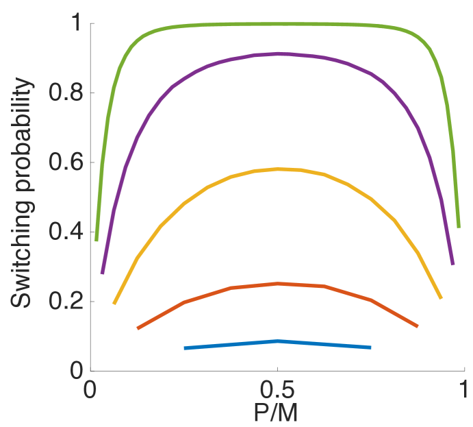
(a) Limiting log-Normal

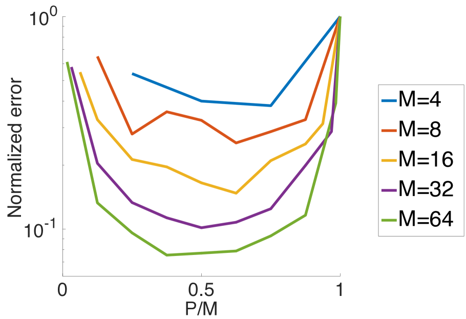
(b) Gaussian state space model

Figure 1: a) Estimation of switching probability for different choices of P and M assuming the log-Normal limiting distribution for $\hat{Z}_{m}$ with $\sigma=3$. b) Median error in mean estimate for different choices of P and M over 10 different synthetic datasets of the linear Gaussian state space model given in (12) after 1000 MCMC iterations. Here errors are normalized by the error of a multi-start PG sampler which is a special case of iPMCMC for which $P=M$ (see Section 4).

In practice we also see that best results are achieved when $P$ makes up roughly half of the nodes, see Figure 1(b) for performance on the state space model introduced in (12). Note also that the accuracy seems to be fairly robust with respect to the choice of $P$. Based on these results, we set the value of $P=\frac{M}{2}$ for the rest of our experiments.

4 Experiments

To demonstrate the empirical performance of iPMCMC we report experiments on two state space models. Although both the models considered are Markovian, we emphasise that iPMCMC goes far beyond this and can be applied to arbitrary graphical models. We will focus our comparison on the trivially distributed alternatives, whereby $M$ independent PMCMC samplers are run in parallel–these are PG, particle independent Metropolis-Hastings (PIMH) Andrieu et al. (2010) and the alternate move PG sampler (APG) Holenstein (2009). Comparisons to other alternatives, including independent SMC, serialized implementations of PG and PIMH, and running a mixture of independent PG and PIMH samplers, are provided in Appendix D. None outperformed the methods considered here, with the exception of running a serialized PG implementation with an increased number of particles, requiring significant additional memory ($O(MN)$ as opposed to $O(M+N)$).

In PIMH a new particle set is proposed at each MCMC step using an independent SMC sweep, which is then either accepted or rejected using the standard Metropolis-Hastings acceptance ratio. APG interleaves PG steps with PIMH steps in an attempt to overcome the issues caused by path degeneracy in PG. We refer to the trivially distributed versions of these algorithms as multi-start PG, PIMH and APG respectively (mPG, mPIMH and mAPG). We use Rao-Blackwellization, as described in 3.2, to average over all the generated particles for all methods, weighting the independent Markov chains equally for mPG, mPIMH and mAPG. We note that mPG is a special case of iPMCMC for which $P=M$. For simplicity, multinomial resampling was used in the experiments, with the prior transition distribution of the latent variables taken for the proposal. $M=32$ nodes and $N=100$ particles were used unless otherwise stated. Initialization of the retained particles for iPMCMC and mPG was done by using standard SMC sweeps.

4.1 Linear Gaussian State Space Model

We first consider a linear Gaussian state space model (LGSSM) with 3 dimensional latent states $x_{1:T}$, 20 dimensional observations $y_{1:T}$ and dynamics given by

$$x_{1} \sim\mathcal{N}\left(\mu,V\right)$$ (12a)

$$x_{t} =\alpha x_{t-1}+\delta_{t-1}\quad \delta_{t-1}\sim\mathcal{N}\left(0,\Omega\right)$$ (12b)

$$y_{t} =\beta x_{t}+\varepsilon_{t}\quad \varepsilon_{t}\sim\mathcal{N}\left(0,\Sigma\right).$$ (12c)

We set $\mu=[0,1,1]^{T}$, $V=0.1\;\mathbf{I}$, $\Omega=\mathbf{I}$ and $\Sigma=0.1\;\mathbf{I}$ where $\mathbf{I}$ represents the identity matrix. The constant transition matrix, $\alpha$, corresponds to successively applying rotations of $\frac{7\pi}{10}$, $\frac{3\pi}{10}$ and $\frac{\pi}{20}$ about the first, second and third dimensions of $x_{t-1}$ respectively followed by a scaling of $0.99$ to ensure that the dynamics remain stable. A total of 10 different synthetic datasets of length $T=50$ were generated by simulating from (12a)–(12c), each with a different emission matrix $\beta$ generated by sampling each column independently from a symmetric Dirichlet distribution with concentration parameter 0.2.

Figure 2(a) shows convergence in the estimate of the latent variable means to the ground-truth solution for iPMCMC and the benchmark algorithms as a function of MCMC iterations. It shows that iPMCMC comfortably outperforms the alternatives from around 200 iterations onwards, with only iPMCMC and mAPG demonstrating behaviour consistent with the Monte Carlo convergence rate, suggesting that mPG and mPIMH are still far from the ergodic regime. Figure 2(b) shows the same errors after $10^{4}$ MCMC iterations as a function of position in state sequence. This demonstrates that iPMCMC outperformed all the other algorithms for the early stages of the state sequence, for which mPG performed particularly poorly. Toward the end of state sequence, iPMCMC, mPG and mAPG all gave similar performance, whilst that of mPIMH was significantly worse.

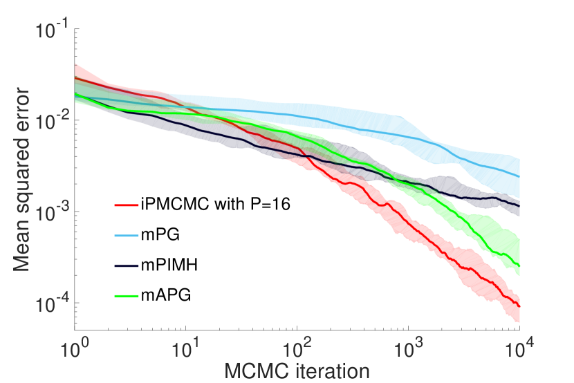
(a) Convergence in mean for full sequence

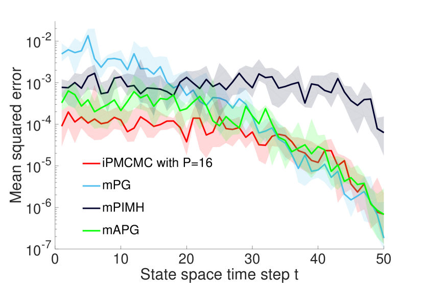
(b) Final error in mean for latent marginals

Figure 2: Mean squared error averaged over all dimensions and steps in the state sequence as a function of MCMC iterations (left) and mean squared error after $10^{4}$ iterations averaged over dimensions as function of position in the state sequence (right) for (12) with 50 time sequences. The solid line shows the median error across the 10 tested synthetic datasets, while the shading shows the upper and lower quartiles. Ground truth was calculated using the Rauch–Tung–Striebel smoother algorithm Rauch et al. (1965).

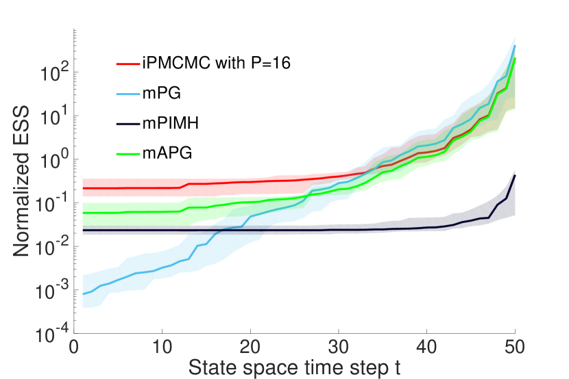
(a) LGSSM

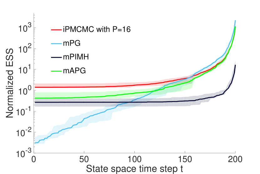
(b) NLSSM

Figure 3: Normalized effective sample size (NESS) for LGSSM (left) and NLSSM (right).

4.2 Nonlinear State Space Model

We next consider the one dimensional nonlinear state space model (NLSSM) considered by, among others, Gordon et al. (1993); Andrieu et al. (2010)

$$x_{1} \sim\mathcal{N}\left(\mu,v^{2}\right)$$ (13a)

$$x_{t} =\frac{x_{t-1}}{2}+25\frac{x_{t-1}}{1+x_{t-1}^{2}}+8\cos\left(1.2t\right)+\delta_{t-1}$$ (13b)

$$y_{t} =\frac{{x_{t}}^{2}}{20}+\varepsilon_{t}$$ (13c)

where $\delta_{t-1}\sim\mathcal{N}\left(0,\omega^{2}\right)$ and $\varepsilon_{t}\sim\mathcal{N}\left(0,\sigma^{2}\right)$. We set the parameters as $\mu=0$, $v=\sqrt{5}$, $\omega=\sqrt{10}$ and $\sigma=\sqrt{10}$. Unlike the LGSSM, this model does not have an analytic solution and therefore one must resort to approximate inference methods. Further, the multi-modal nature of the latent space makes full posterior inference over $x_{1:T}$ challenging for long state sequences.

Figure 4: Histograms of generated samples at $t=1,100,\text{ and }200$ for a single dataset generated from (13) with $T=200$. Dashed red line shows an approximate estimate of the ground truth, found by running a kernel density estimator on the combined samples from a small number of independent SMC sweeps, each with $10^{7}$ particles.

To examine the relative mixing of iPMCMC we calculate an effective sample size (ESS) for different steps in the state sequence. In order to calculate the ESS, we condensed identical samples as done in for example van de Meent et al. (2015). Let

$$u_{t}^{k}\in\{x_{t,m}^{i}[r]\}^{i=1:N,r=1:R}_{m=1:M},\quad\forall k\in 1\dots K,\;t\in 1\dots T$$

denote the unique samples of $x_{t}$ generated by all the nodes and sweeps of particular algorithm after $R$ iterations, where $K$ is the total number of unique samples generated. The weight assigned to these unique samples, $v_{t}^{k}$, is given by the combined weights of all particles for which $x_{t}$ takes the value $u_{t}^{k}$:

$$v_{t}^{k}=\sum_{r=1}^{R}\sum_{m=1}^{M}\sum_{i=1}^{N}\bar{w}_{t,m}^{i,r}\eta_{m}^{r}\delta_{x_{t,m}^{i}[r]}(u_{t}^{k})$$ (14)

where $\delta_{x_{t,m}^{i}[r]}(u_{t}^{k})$ is the Kronecker delta function and $\eta_{m}^{r}$ is a node weight. For iPMCMC the node weight is given by as per the Rao-Blackwellized estimator described in Section 3.2. For mPG and mPIMH, $\eta_{m}^{r}$ is simply $\frac{1}{RM}$, as samples from the different nodes are weighted equally in the absence of interaction. Finally we define the effective sample size as $\text{ESS}_{t}=\left(\textstyle\sum_{k=1}^{K}\left(v_{t}^{k}\right)^{2}\right)^{-1}$.

Figure 3 shows the ESS for the LGSSM and NLSSM as a function of position in the state sequence. For this, we omit the samples generated by the initialization step as this SMC sweep is common to all the tested algorithms. We further normalize by the number of MCMC iterations so as to give an idea of the rate at which unique samples are generated. These show that for both models the ESS of iPMCMC, mPG and mAPG is similar towards the end of the space sequence, but that iPMCMC outperforms all the other methods at the early stages. The ESS of mPG was particularly poor at early iterations. PIMH performed poorly throughout, reflecting the very low observed acceptance ratio of around $7.3\%$ on average.

It should be noted that the ESS is not a direct measure of performance for these models. For example, the equal weighting of nodes is likely to make the ESS artificially high for mPG, mPIMH and mAPG, when compared with methods such as iPMCMC that assign a weighting to the nodes at each iteration. To acknowledge this, we also plot histograms for the marginal distributions of a number of different position in the state sequence as shown in Figure 4. These confirm that iPMCMC and mPG have similar performance at the latter state sequence steps, whilst iPMCMC is superior at the earlier stages, with mPG producing almost no more new samples than those from the initialization sweep due to the degeneracy. The performance of PIMH was consistently worse than iPMCMC throughout the state sequence, with even the final step exhibiting noticeable noise.

5 Discussion and Future Work

The iPMCMC sampler overcomes degeneracy issues in PG by allowing the newly sampled particles from SMC nodes to replace the retained particles in CSMC nodes. Our experimental results demonstrate that, for the models considered, this switching in rate is far higher than the rate at which PG generates fully independent samples. Moreover, the results in Figure 1(b) suggest that the degree of improvement over an mPG sampler with the same total number of nodes increases with the total number of nodes in the pool.

The mAPG sampler performs an accept reject step that compares the marginal likelihood estimate of a single CSMC sweep to that of a single SMC sweep. In the iPMCMC sampler the CSMC estimate of the marginal likelihood is compared to a population sample of SMC estimates, resulting in a higher probability that at least one of the SMC nodes will become a CSMC node.

Since the original PMCMC paper in 2010 there have been several papers studying (Chopin and Singh, 2015; Lindsten et al., 2015) and improving upon the basic PG algorithm. Key contributions to combat the path degeneracy effect are backward simulation (Whiteley et al., 2010; Lindsten and Schön, 2013) and ancestor sampling (Lindsten et al., 2014). These can also be used to improve the iPMCMC method ever further.

A Proof of Theorem 1

The proof follows similar ideas as Andrieu et al. (2010). We prove that the interacting particle Markov chain Monte Carlo sampler is in fact a standard partially collapsed Gibbs sampler (Van Dyk and Park, 2008) on an extended space ${\Upsilon:=\mathsf{X}^{\otimes MTN}\times[N]^{\otimes M(T-1)N}\times[M]^{\otimes P}\times[N]^{\otimes P}}$.

Proof  Assume the setup of Section 3. With $\tilde{\pi}(\cdot)$ with as per (1), we will show that the Gibbs sampler on the extended space, $\Upsilon$, defined as follows

$$\mathbf{\xi}_{1:M}\backslash\{\mathbf{x}_{c_{1:P}}^{b_{1:P}},\mathbf{b}_{c_{1:P}}\}~{} \sim\tilde{\pi}(~{}\cdot~{}|\mathbf{x}_{c_{1:P}}^{b_{1:P}},\mathbf{b}_{c_{1:P}},c_{1:P},b_{1:P}),$$ (15a)

$$c_{j} \sim\tilde{\pi}(~{}\cdot~{}|\mathbf{\xi}_{1:M},c_{1:P\backslash j}),~{}~{}j=1,\ldots,P,$$ (15b)

$$b_{j} \sim\tilde{\pi}(~{}\cdot~{}|\mathbf{\xi}_{1:M},c_{1:P}),~{}~{}j=1,\ldots,P,$$ (15c)

is equivalent to the iPMCMC method in Algorithm 3.

First, the initial step (15a) corresponds to sampling from

$$\tilde{\pi}(\mathbf{\xi}_{1:M} \backslash\{\mathbf{x}_{c_{1:P}}^{b_{1:P}},\mathbf{b}_{c_{1:P}}\}|\mathbf{x}_{c_{1:P}}^{b_{1:P}},\mathbf{b}_{c_{1:P}},c_{1:P},b_{1:P})=$$

$$\prod_{\begin{subarray}{c}m=1\\ m\notin c_{1:P}\end{subarray}}^{M}q_{\text{SMC}}\left(\mathbf{\xi}_{m}\right)\prod_{j=1}^{P}q_{\text{CSMC}}\left(\mathbf{\xi}_{c_{j}}\backslash\{\mathbf{x}_{c_{j}}^{b_{j}},\mathbf{b}_{c_{j}}\}\mid\mathbf{x}_{c_{j}}^{b_{j}},\mathbf{b}_{c_{j}},c_{j},b_{j}\right).$$

This, excluding the conditional trajectories, just corresponds to steps 3–4 in Algorithm 3, i.e. running $P$ CSMC and $M-P$ SMC algorithms independently.

We continue with a reformulation of (1) which will be useful to prove correctness for the other two steps

$$\tilde{\pi} (\mathbf{\xi}_{1:M},c_{1:P},b_{1:P})$$

$$=\frac{1}{\binom{M}{P}}\prod_{m=1}^{M}q_{\text{SMC}}\left(\mathbf{\xi}_{m}\right)\cdot\prod_{j=1}^{P}\left[\mathds{1}_{c_{j}\notin c_{1:j-1}}\bar{w}_{T,c_{j}}^{b_{j}}\pi_{T}\left(\mathbf{x}_{c_{j}}^{b_{j}}\right)\frac{q_{\text{CSMC}}\left(\mathbf{\xi}_{c_{j}}\backslash\{\mathbf{x}_{c_{j}}^{b_{j}},\mathbf{b}_{c_{j}}\}\mid\mathbf{x}_{c_{j}}^{b_{j}},\mathbf{b}_{c_{j}},c_{j},b_{j}\right)}{N^{T}\bar{w}_{T,c_{j}}^{b_{j}}q_{\text{SMC}}\left(\mathbf{\xi}_{c_{j}}\right)}\right]$$

$$=\frac{1}{\binom{M}{P}}\prod_{m=1}^{M}q_{\text{SMC}}\left(\mathbf{\xi}_{m}\right)\cdot\prod_{j=1}^{P}\frac{\hat{Z}_{c_{j}}}{Z}\mathds{1}_{c_{j}\notin c_{1:j-1}}\bar{w}_{T,c_{j}}^{b_{j}}.$$ (16)

Furthermore, we note that by marginalising (collapsing) the above reformulation, i.e. (A), over $b_{1:P}$ we get

$$\tilde{\pi}(\mathbf{\xi}_{1:M},c_{1:P}) =\frac{1}{\binom{M}{P}}\prod_{m=1}^{M}q_{\text{SMC}}\left(\mathbf{\xi}_{m}\right)\prod_{j=1}^{P}\frac{\hat{Z}_{c_{j}}}{Z}\mathds{1}_{c_{j}\notin c_{1:j-1}}.$$

From this it is easy to see that $\tilde{\pi}(c_{j}|\mathbf{\xi}_{1:M},c_{1:P\backslash j})=\hat{\zeta}_{c_{j}}^{j}$, which corresponds to sampling the conditional node indices, i.e. step 6 in Algorithm 3. Finally, from (A) we can see that simulating $b_{1:P}$ can be done independently as follows

$$\tilde{\pi}(b_{1:P}|\mathbf{\xi}_{1:M},c_{1:P})=\frac{\tilde{\pi}(b_{1:P},\mathbf{\xi}_{1:M},c_{1:P})}{\tilde{\pi}(\mathbf{\xi}_{1:M},c_{1:P})}=\prod_{j=1}^{P}\bar{w}_{T,c_{j}}^{b_{j}}.$$

This corresponds to step 7 in the iPMCMC sampler, Algorithm 3. So the procedure defined by (15) is a partially collapsed Gibbs sampler, derived from (1), and we have shown that it is exactly equal to the iPMCMC sampler described in Algorithm 3.  

B Using All Particles

The Monte Carlo estimator is given by

$$\mathbb{E}[f(\mathbf{x})] \approx\frac{1}{RP}\sum_{r=1}^{R}\sum_{j=1}^{P}f(\mathbf{x}_{j}^{\prime}[r])$$

$$=\frac{1}{R}\sum_{r=1}^{R}\frac{1}{P}\sum_{j=1}^{P}f(\mathbf{x}_{j}^{\prime}[r]),$$ (17)

where we can note that $\mathbf{x}_{j}^{\prime}[r]=\mathbf{x}_{c_{j}}^{b_{j}}$ from the internal particle system at iteration $r$. We can however make use of all particles to estimate expectations of interest by, for each MCMC iteration $r$, averaging over the sampled conditional node indices $c_{1:P}$ and corresponding particle indices $b_{1:P}$. This procedure is referred to as a Rao-Blackwellization of a statistical estimator and is (in terms of variance) never worse than the original one, and often much better. For iteration $r$ we need to calculate the following

$$\frac{1}{P}\sum_{j=1}^{P}f(\mathbf{x}_{j}^{\prime}[r])=\frac{1}{P}\sum_{j=1}^{P}f(\mathbf{x}_{c_{j}}^{b_{j}}),$$

where we can Rao-Blackwellize the selection of the retained particle along with each individual Gibbs update as following

$$\frac{1}{P}\sum_{j=1}^{P}\mathbb{E}_{c_{j},b_{j}|\xi_{1:M},c_{1:P\backslash j}}\left[f(\mathbf{x}_{c_{j}}^{b_{j}})\right]= \frac{1}{P}\sum_{j=1}^{P}\mathbb{E}_{c_{j}|\xi_{1:M},c_{1:P\backslash j}}\left[\sum_{i=1}^{N}\bar{w}_{T,c_{j}}^{i}f(\mathbf{x}_{c_{j}}^{i})\right]$$

$$= \frac{1}{P}\sum_{j=1}^{P}\sum_{i=1}^{N}\mathbb{E}_{c_{j}|\xi_{1:M},c_{1:P\backslash j}}\left[\bar{w}_{T,c_{j}}^{i}f(\mathbf{x}_{c_{j}}^{i})\right]$$

$$= \frac{1}{P}\sum_{j=1}^{P}\sum_{i=1}^{N}\sum_{m=1}^{M}\hat{\zeta}_{m}^{j}\bar{w}_{T,m}^{i}f(\mathbf{x}_{m}^{i})$$

$$= \frac{1}{P}\sum_{j=1}^{P}\sum_{m=1}^{M}\hat{\zeta}_{m}^{j}\sum_{i=1}^{N}\bar{w}_{T,m}^{i}f(\mathbf{x}_{m}^{i})$$

$$= \frac{1}{P}\sum_{m=1}^{M}\left[\left(\sum_{j=1}^{P}\hat{\zeta}_{m}^{j}\right)\cdot\left(\sum_{i=1}^{N}\bar{w}_{T,m}^{i}f(\mathbf{x}_{m}^{i})\right)\right]$$

where we have made use of the knowledge that the internal particle system $\{(\mathbf{x}_{m}^{i},\bar{w}_{T,m}^{i})\}$ does not change between Gibbs updates of the $c_{j}$’s, whereas the $\hat{\zeta}_{m}^{j}$ do. We emphasise that this is a separate Rao-Blackwellization of each Gibbs update of the conditional node indices, such that each is conditioned upon the actual update made at $j-1$, rather than a simultaneous Rao-Blackwellization of the full batch of $P$ updates. Though the latter also has analytic form and should theoretically be lower variance, it suffers from inherent numerical instability and so is difficult to calculate in practise. We found that empirically there was not a noticeable difference between the performance of the two procedures. Furthermore, one can always run additional Gibbs updates on the $c_{j}$’s and obtain an improve estimate on the relative sample weightings if desired.

C Choosing $P$

For the purposes of this study we assume, without loss of generality, that the indices for the conditional nodes are always $c_{1:P}=\{1,\ldots,P\}$. Then we can show that the probability of the event that at least one conditional nodes switches with an unconditional is given by

$$\mathbb{P}(\{\text{switch}\})=1-\mathbb{E}\left[\prod_{j=1}^{P}\frac{\hat{Z}_{j}}{\hat{Z}_{j}+\sum_{m=P+1}^{M}\hat{Z}_{m}}\right].$$ (18)

Now, there are some asymptotic (and experimental) results (Pitt et al., 2012; Bérard et al., 2014; Doucet et al., 2015) that indicate that a decent approximation for the distribution of the log of the normalisation constant estimates is Gaussian. This would mean the distributions of the conditional and unconditional normalisation constant estimates with variance $\sigma^{2}$ can be well-approximated as follows

$$\log\left(\frac{\hat{Z}_{j}}{Z}\right) \sim\mathcal{N}(\frac{\sigma^{2}}{2},\sigma^{2}),\quad j=1,\ldots,P,$$ (19)

$$\log\left(\frac{\hat{Z}_{m}}{Z}\right) \sim\mathcal{N}(-\frac{\sigma^{2}}{2},\sigma^{2}),\quad m=P+1,\ldots,M.$$ (20)

A straight-forward Monte Carlo estimation of the switching probability, i.e. $\mathbb{P}(\{\text{switch}\})$, can be seen in Figure 5 for various settings of $\sigma$ and $M$. These results seem to indicate that letting $P\approx M/2$ maximises the probability of switching.

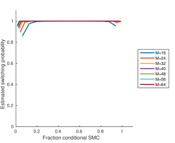
(a) $\sigma=1$

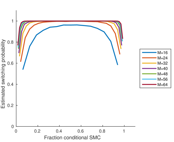
(b) $\sigma=2$

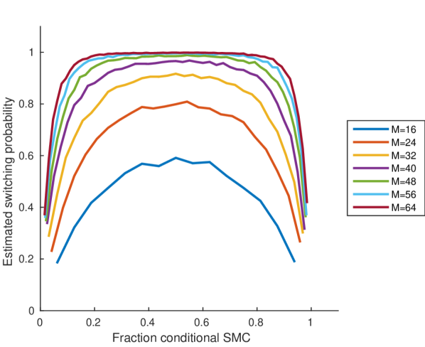
(c) $\sigma=3$

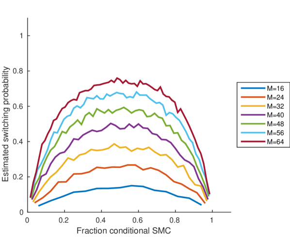
(d) $\sigma=4$

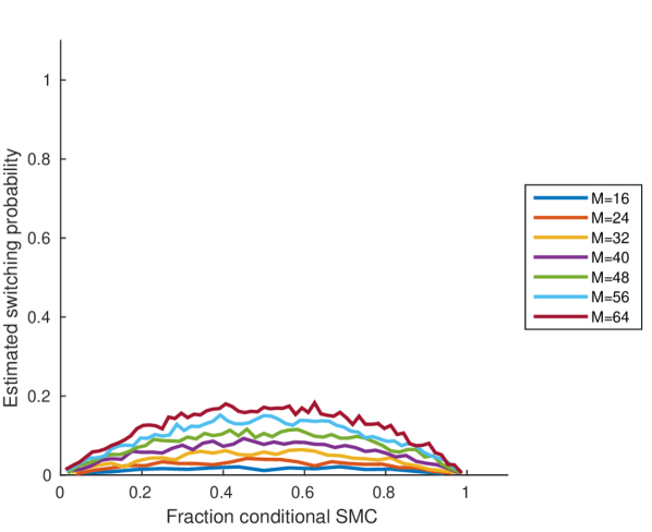
(e) $\sigma=5$

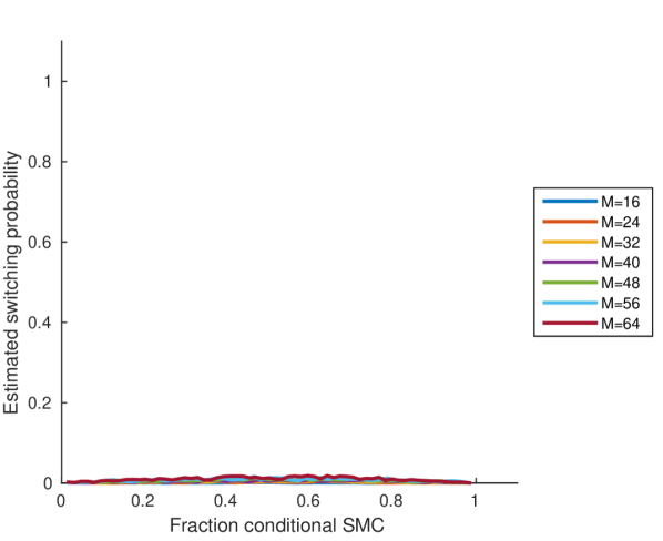
(f) $\sigma=6$

Figure 5: Estimation of switching probability for various settings of $\sigma$ and $M$.

D Additional Results Figures

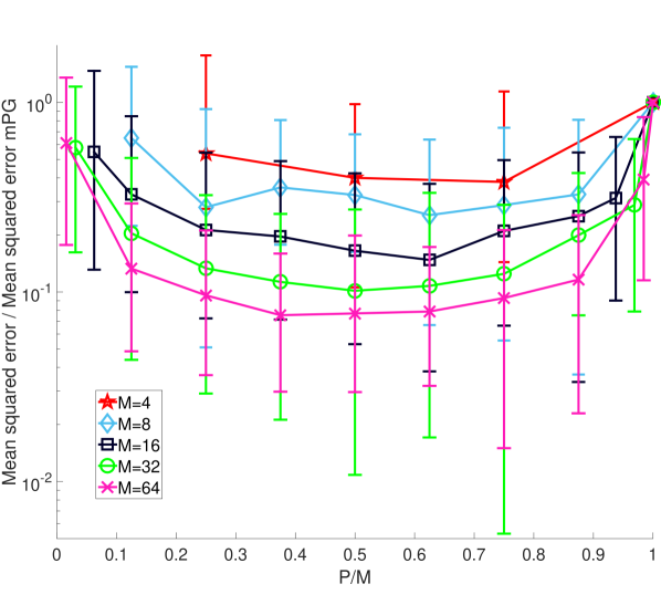
(a) Mean

(b) Standard Deviation

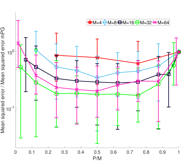
(c) Skewness

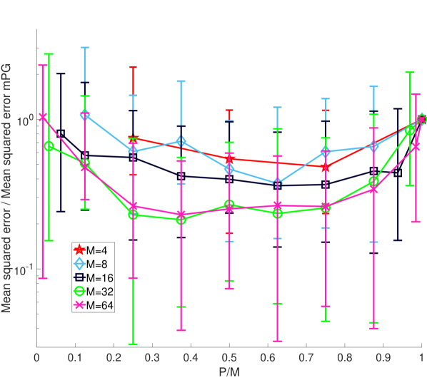
(d) Kurtosis

Figure 6: Median error in marginal moment estimates with different choices of P and M over 10 different synthetic datasets of the linear Gaussian state space model given in (10) after 1000 MCMC iterations. Errors are normalized by the error of a multi-start PG sampler which is a special case of iPMCMC for which $P=M$ (see Section 4). Error bars show the lower and upper quartiles for the errors. It can be seen that for all the moments then $P/M\approx 1/2$ give the best performance. For the mean and standard deviation estimates, the accuracy relative to the non-interacting distribution case $P=M$ shows a clear increase with $M$. This effect is also seen for the skewness and excess kurtosis estimates except for the distinction between the $M=32$ and $M=64$ cases. This may be because these metric are the same for the prior and the posterior such that good results for these metric might be achievable even when the samples give a poor match to the true posterior.

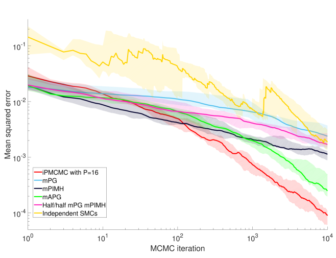
(a) Convergence in mean

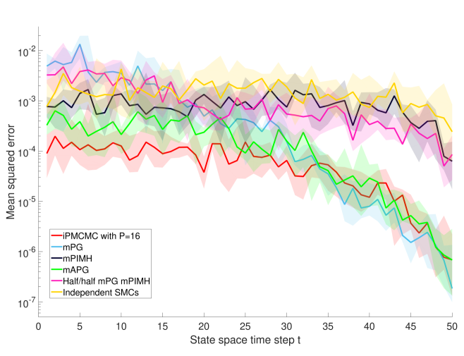
(b) Final error in mean

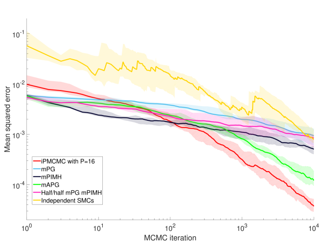
(c) Convergence in standard deviation

(d) Final error in standard deviation

Figure 7: Mean squared error in latent variable mean and standard deviation averaged over all dimensions of the LGSSM as a function of MCMC iteration (left) and position in the state sequence (right) for a selection of paraellelizable SMC and PMCMC methods. See figure 3 in main paper for more details.

(a) Convergence in skewness

(b) Final error in skewness

(c) Convergence in kurtosis

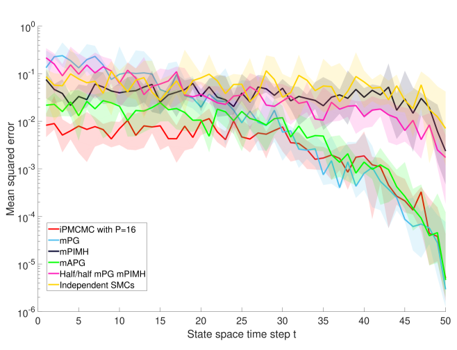
(d) Final error in kurtosis

Figure 8: Mean squared error in latent variable skewness and kurtosis averaged over all dimensions of the LGSSM as a function of MCMC iteration (left) and position in the state sequence (right) for a selection of paraellelizable SMC and PMCMC methods. See figure 3 in main paper for more details.

(a) Convergence in mean

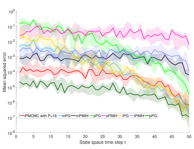
(b) Final error in mean

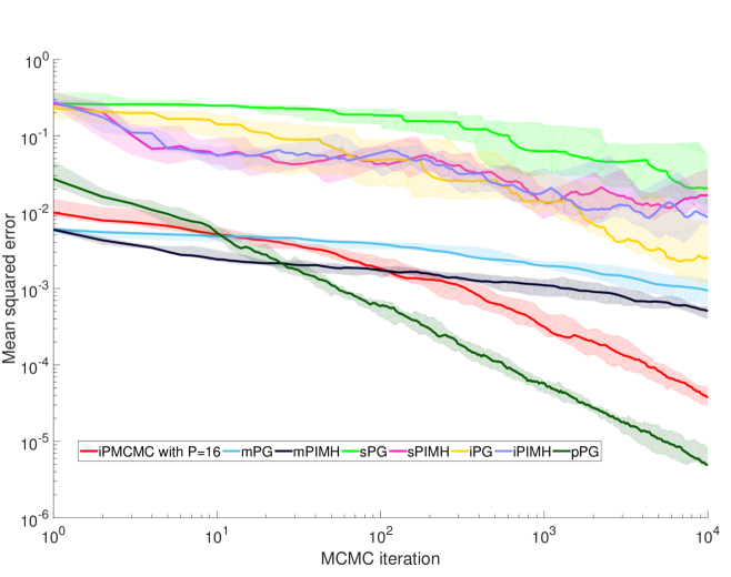
(c) Convergence in standard deviation

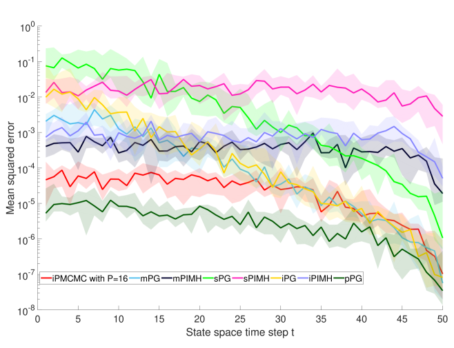
(d) Final error in standard deviation

Figure 9: Mean squared error in latent variable mean and standard deviation averaged of all dimensions of the LGSSM as a function of MCMC iteration (left) and position in the state sequence (right) for iPMCMC, mPG, mPIMH and a number of serialized variants. Key for legends: sPG = single PG chain, sPIMH = single PIMH chain, iPG = single PG chain run 32 times longer, iPIMH = single PIMH chain run 32 times longer and pPG = single PG with 32 times more particles. For visualization purposes, the chains with extra iterations have had the number of MCMC iterations normalized by 32 so that the different methods represent equivalent total computational budget.

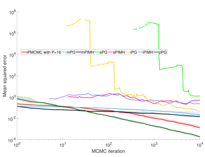
(a) Convergence in skewness

(b) Final error in skewness

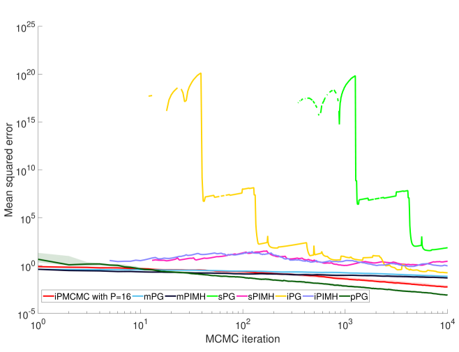
(c) Convergence in kurtosis

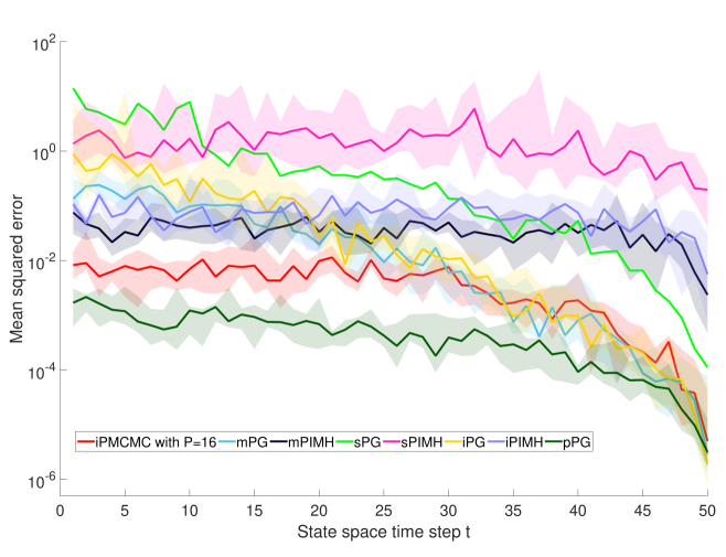
(d) Final error in kurtosis

Figure 10: Mean squared error in latent variable skewness and kurtosis averaged of all dimensions of the LGSSM as a function of MCMC iteration (left) and position in the state sequence (right) for iPMCMC, mPG, mPIMH and a number of serialized variants. Key for legends: sPG = single PG chain, sPIMH = single PIMH chain, iPG = single PG chain run 32 times longer, iPIMH = single PIMH chain run 32 times longer and pPG = single PG with 32 times more particles. For visualization purposes, the chains with extra iterations have had the number of MCMC iterations normalized by 32 so that the different methods represent equivalent total computational budget.

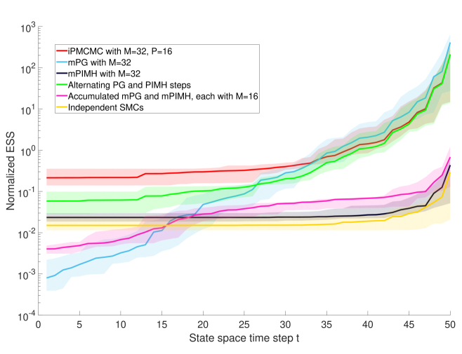
(a) ESS of distributed methods for LGSSM

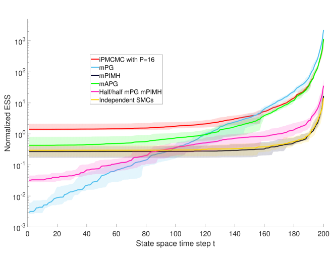
(b) ESS of distributed methods for NLSSM

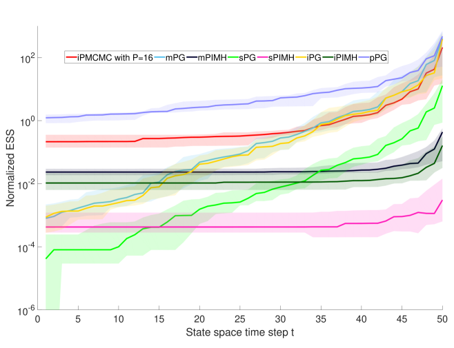
(c) ESS comparison to series equivalents for LGSSM

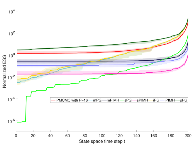
(d) ESS comparison to series equivalents for NLSSM

Figure 11: Normalized effective sample size for LGSSM (left) and NLSSM (right) for a number of distributed and series models. Key for legends: sPG = single PG chain, sPIMH = single PIMH chain, iPG = single PG chain run 32 times longer, iPIMH = single PIMH chain run 32 times longer and pPG = single PG with 32 times more particles.

References

- Andrieu et al. (2010) Christophe Andrieu, Arnaud Doucet, and Roman Holenstein. Particle Markov chain Monte Carlo methods. Journal of the Royal Statistical Society: Series B (Statistical Methodology), 72(3):269–342, 2010. ISSN 1467-9868.
- Bérard et al. (2014) Jean Bérard, Pierre Del Moral, and Arnaud Doucet. A lognormal central limit theorem for particle approximations of normalizing constants. Electronic Journal of Probability, 19(94):1–28, 2014.
- Chopin and Singh (2015) Nicolas Chopin and Sumeetpal S. Singh. On particle Gibbs sampling. Bernoulli, 21(3):1855–1883, 08 2015. doi: 10.3150/14-BEJ629.
- Doucet et al. (2001) Arnaud Doucet, Nando de Freitas, and Neil Gordon. Sequential Monte Carlo methods in practice. Springer Science & Business Media, 2001.
- Doucet et al. (2015) Arnaud Doucet, Michael Pitt, George Deligiannidis, and Robert Kohn. Efficient implementation of Markov chain Monte Carlo when using an unbiased likelihood estimator. Biometrika, page asu075, 2015.
- Everitt (2012) Richard G. Everitt. Bayesian parameter estimation for latent Markov random fields and social networks. Journal of Computational and Graphical Statistics, 21(4):940–960, 2012.
- Gordon et al. (1993) Neil J Gordon, David J Salmond, and Adrian FM Smith. Novel approach to nonlinear/non-Gaussian Bayesian state estimation. IEE Proceedings F (Radar and Signal Processing), 140(2):107–113, 1993.
- Holenstein (2009) Roman Holenstein. Particle Markov chain Monte Carlo. PhD thesis, The University Of British Columbia (Vancouver, 2009.
- Huggins and Roy (2015) Jonathan H. Huggins and Daniel M. Roy. Convergence of sequential Monte Carlo-based sampling methods. ArXiv e-prints, arXiv:1503.00966v1, March 2015.
- Lindsten and Schön (2013) Fredrik Lindsten and Thomas B Schön. Backward simulation methods for Monte Carlo statistical inference. Foundations and Trends in Machine Learning, 6(1):1–143, 2013.
- Lindsten et al. (2014) Fredrik Lindsten, Michael I. Jordan, and Thomas B. Schön. Particle Gibbs with ancestor sampling. Journal of Machine Learning Research, 15:2145–2184, june 2014.
- Lindsten et al. (2015) Fredrik Lindsten, Randal Douc, and Eric Moulines. Uniform ergodicity of the particle Gibbs sampler. Scandinavian Journal of Statistics, 42(3):775–797, 2015.
- Naesseth et al. (2014) Christian A Naesseth, Fredrik Lindsten, and Thomas B Schön. Sequential Monte Carlo for graphical models. In Advances in Neural Information Processing Systems 27, pages 1862–1870. Curran Associates, Inc., 2014.
- Naesseth et al. (2015) Christian A. Naesseth, Fredrik Lindsten, and Thomas B Schön. Nested sequential Monte Carlo methods. In The 32nd International Conference on Machine Learning, volume 37 of JMLR W&CP, pages 1292–1301, Lille, France, jul 2015.
- Pitt et al. (2012) Michael K Pitt, Ralph dos Santos Silva, Paolo Giordani, and Robert Kohn. On some properties of Markov chain Monte Carlo simulation methods based on the particle filter. Journal of Econometrics, 171(2):134–151, 2012.
- Rainforth et al. (2016) Tom Rainforth, Christian A Naesseth, Fredrik Lindsten, Brooks Paige, Jan-Willem van de Meent, Arnaud Doucet, and Frank Wood. Interacting particle Markov chain Monte Carlo. In Proceedings of the 33rd International Conference on Machine Learning, volume 48 of JMLR: W&CP, 2016.
- Rauch et al. (1965) Herbert E Rauch, CT Striebel, and F Tung. Maximum likelihood estimates of linear dynamic systems. AIAA journal, 3(8):1445–1450, 1965.
- Robert and Casella (2013) Christian Robert and George Casella. Monte Carlo statistical methods. Springer Science & Business Media, 2013.
- Tripuraneni et al. (2015) Nilesh Tripuraneni, Shixiang Gu, Hong Ge, and Zoubin Ghahramani. Particle Gibbs for infinite hidden Markov Models. In Advances in Neural Information Processing Systems 28, pages 2386–2394. Curran Associates, Inc., 2015.
- Valera et al. (2015) Isabel Valera, Fran Francisco, Lennart Svensson, and Fernando Perez-Cruz. Infinite factorial dynamical model. In Advances in Neural Information Processing Systems 28, pages 1657–1665. Curran Associates, Inc., 2015.
- van de Meent et al. (2015) Jan-Willem van de Meent, Hongseok Yang, Vikash Mansinghka, and Frank Wood. Particle Gibbs with ancestor sampling for probabilistic programs. In Proceedings of the 18th International conference on Artificial Intelligence and Statistics, pages 986–994, 2015.
- Van Dyk and Park (2008) David A Van Dyk and Taeyoung Park. Partially collapsed Gibbs samplers: Theory and methods. Journal of the American Statistical Association, 103(482):790–796, 2008.
- Whiteley et al. (2010) Nick Whiteley, Christophe Andrieu, and Arnaud Doucet. Efficient Bayesian inference for switching state-space models using discrete particle Markov chain Monte Carlo methods. ArXiv e-prints, arXiv:1011.2437, 2010.
- Whiteley et al. (2016) Nick Whiteley, Anthony Lee, and Kari Heine. On the role of interaction in sequential Monte Carlo algorithms. Bernoulli, 22(1):494–529, 02 2016.
- Wood et al. (2014) Frank Wood, Jan Willem van de Meent, and Vikash Mansinghka. A new approach to probabilistic programming inference. In Proceedings of the 17th International conference on Artificial Intelligence and Statistics, pages 2–46, 2014.