Practical Introduction to Clustering Data

Abstract

Data clustering is an approach to seek for structure in sets of complex data, i.e., sets of “objects”. The main objective is to identify groups of objects which are similar to each other, e.g., for classification. Here, an introduction to clustering is given and three basic approaches are introduced: the k-means algorithm, neighbour-based clustering, and an agglomerative clustering method. For all cases, C source code examples are given, allowing for an easy implementation.

This introduction originates (with a couple of modifications) from section 8.5.6 of the book: A.K. Hartmann, Big Practical Guide to Computer Simulations, World-Scientifc, Singapore (2015).

1 Introduction

Often one wants to find similarities in a set of $n$ objects, characterized by “feature vectors”. We assume that the data is given by $n$ $d$-dimensional real-valued data points $\{{\underline{x}}^{(i)}\}$ ($i=0,\ldots,n-1$), with each data point ${\underline{x}}^{(i)}=(x_{1}^{(i)},\ldots,x_{d}^{(i)})^{T}$. Furthermore, let the data exhibit some substructure, i.e., one can organize the data into groups, called clusters, such that the objects within the groups are more similar to each other compared to objects belonging to different groups. Note that this is not a precise definition. In fact, a good definition does not exisit. Thus, what is a good clustering always depends on the application and on the data. This is already illustrated by the two sample data sets A and B, which are shown in Fig. 1. For a detailed discussion of clustering see, e.g., Ref. [Jain and Dubes (1988)]. Here, we discuss three approaches, the k-means algorithm, neighbor-based clustering, and an agglomerative clusering method.

All C source code examples can be found in the file cluster.c (main programm with simple examples plus subroutines). To compile the program also the files graphs.c, list.c, and graphs_comps.c plus corresponding header files must be present. These files implement simple data structures and algorithms for representing graphs, based on neighbour lists. All files are provided in the with this arXiv submission in the anc directory. Note that also the GNU Scientific library has to be installed. [Galassi et al. (2006)]. A sample compile command is

cc -o cluster cluster.c graphs.c  list.c graph_comps.c \
   -lgsl -lgslcblas -lm -Wall

For using the main program, please have a look at main() function in the cluster.c file. Note that in cluster.c also two functions cluster_test_data1() and cluster_test_data2() are included, which generate the sample data sets used throughout this introduction.

2 $k$-means Clustering

Figure 1: Two sample sets A ($n=200$, left) and B ($n=200$, right) for sets of two-dimensional data points, which will subsequently be used to test clustering algorithms, aiming at identifying subsets of similar data points.

Following the $k$-means approach, one wants to partition the data set into $k$ clusters, $k$ being a somehow given parameter. Below we discuss shortly the influence of the choice of $k$ on the resulting clustering. The $k$-means approach is based on a geometric point of view. Each cluster $c=0\ldots,k-1$ shall be represented by a center vector ${\underline{\xi}}^{(c)}$. Let us assume that each data point with index $i\in\{0,\ldots,n-1\}$ is assigned to some (initially possibly randomly chosen) cluster $c(i)\in\{0,\ldots,k-1\}$.

We calculate the mean-squared difference (or “spread”) $\chi^{2}$ of all data points to the center of its cluster:

$$\chi^{2}=\frac{1}{n}\sum_{i=0}^{n-1}\left({\underline{\xi}}^{(c(i))}-{\underline{x}}^{(i)}\right)^{2}\,.$$

We assume that the best choice of the center vectors and of the assignment to the clusters is the one which minimizes the spread. Thus, for a fixed assignment of data points to clusters and any cluster $c\in\{0,\ldots,k-1\}$ we have for each direction $a\in\{1,\ldots,d\}$ the condition that the partial derivative of the spread with respect to the $a$’th component of the center vector ${\underline{\xi}}^{(c)}$ vanishes:

$$0\stackrel{{\scriptstyle!}}{{=}}\frac{\partial\chi^{2}}{\partial\xi_{a}^{c}}=\frac{2}{n}\sum_{i=0}^{n-1}\delta_{c,c(i)}\left(\xi^{(c(i))}_{a}-x^{(i)}_{a}\right)=2\frac{n_{c}}{n}\xi^{(c)}_{a}-\frac{2}{n}\sum_{i=0}^{n-1}\delta_{c,c(i)}x^{(i)}_{a}\,,$$

where $n_{c}=\sum_{i=0}^{n-1}\delta_{c,c(i)}$ is the size of cluster $c$. Thus, each center vector ${\underline{\xi}}^{(c)}$ is, as the name suggest, the geometric center of the data points assigned to cluster $c$:

$${\underline{\xi}}^{(c)}=\frac{1}{n_{c}}\sum_{i=0}^{n-1}\delta_{c,c(i)}{\underline{x}}^{(i)}\,.$$ (1)

On the other hand, for fixed centers ${\underline{\xi}}^{(c)}$, minimizing $\chi^{2}$ can be achieved by assigning each data point to its closest cluster:

$$c(i)=\operatorname{argmin}_{c=0,\ldots,k-1}\left\{\left({\underline{\xi}}^{(c)}-{\underline{x}}^{(i)}\right)^{2}\right\}\,.$$ (2)

Thus, a very simple algorithm can be obtained by starting with a random assignments of the data points to clusters and then iterating Eqs. (1) and (2) until convergence, e.g., until the the relative change of the center vectors is less than a small given threshold $\epsilon$. Note that this approach does not guarantee a convergence to a solution where the spread $\chi^{2}$ assumes its global minimum. See below for an example.

Next, we discuss a short C implementation of the $k$-means approach. Note that the file cluster.c also contains auxiliary and test functions, like cluster_test_data1() and cluster_test_data2() which generate the test sets A and B, respectively. You can just use the code it as it is, or use it as a starting point for a more refined approach, e.g., by introducing additional weights signifying the importance of the data points. The function cluster_k_means() receives a matrix data, which contains the data points as column vectors, and the number $k$ of clusters. For convenience, we use the data types gsl_vector and gsl_matrix of the GNU Scientific Library (GSL) [Galassi et al. (2006)], see also Sec. 7.3. of Ref. [Hartmann (2015)]. Also we use a GSL random number generator rng for the initial assignment of the data points to the clusters. The function returns an array, which contains for each data point an integer specifying its cluster. The array is created inside the function. Furthermore, the function returns the final spread, via a pointer spread_p which is passed as argument.

int *cluster_k_means(gsl_matrix *data, int k, gsl_rng *rng,
                     double *spread_p)
{
  int *cluster;             /* holds for each point its cluster ID */
  gsl_matrix *center;         /* holds for each cluster its center */
  int *cluster_size;         /* holds for each cluster its #points */
  int dim;           /* number of components of data point vectors */
  int num_points;                         /* number of data points */
  int t, d, c;                                    /* loop counters */
  double spread, spread_old;          /* total distance to centers */
  double dist, dist_min;   /* (minimum) dist. between point/center */
  double diff;            /* lateral distance between point/center */
  int c_min;                 /* center which is closest to a point */
  int do_print = 0;                               /* for debugging */

For initializing, the number num_points of data points and the number dim of entries are take from the GSL matrix data structure (lines 15 and 16). Using this, the array cluster, which is returned, the array cluster_size, which holds for each cluster the number of assigned data points, and a GSL matrix for the centers are allocated (lines 17–19). Also, each data point is assigned initially to a randomly chosen cluster (lines 21,22):

  num_points = data->size2;                          /* initialize */
  dim = data->size1;
  cluster = (int *) malloc(num_points*sizeof(int));
  cluster_size = (int *) malloc(k*sizeof(int));
  center = gsl_matrix_alloc(dim, k);

  for(t=0; t<num_points; t++)    /* intial assignments to clusters */
    cluster[t] = (int) k*gsl_rng_uniform(rng);
  spread = 1e100;
  spread_old = 2e100;

The main loop (lines 25–64) is performed until the spread changes by less than one percent (line 25). In each iteration, for the given assignments of the data points to clusters, the cluster sizes and the cluster centers are updated (lines 27–42) according to Eq. (1). This is achieved by first initializing centers and cluster sizes to zero (lines 27–29), by next iterating over all data points (lines 30–37), and by finally normalizing the centers by the cluster sizes $n_{c}$ (lines 38–42). Note that in C, the entries $1,\ldots,d$ of the data points run from 0 to dim$-1$.

For each iteration, second, for each data point its closest cluster is determined and the spread is recalculated (lines 44–63). This involves in particular iterating for each data point over all cluster centers (lines 48–62), determining the distance between the data point and a center (lines 50–55) and determining the closest center (lines 56–60).

  while ( (spread_old-spread)>0.01*spread_old)        /* main loop */
  {
    gsl_matrix_set_all(center, 0.0);
    for(c=0; c<k; c++)
      cluster_size[c] = 0;
    for(t=0; t<num_points; t++)               /* determine centers */
    {
      cluster_size[cluster[t]]++;
      for(d=0; d<dim; d++)
        gsl_matrix_set(center, d, cluster[t],
                       gsl_matrix_get(center, d, cluster[t])+
                       gsl_matrix_get(data, d, t));
    }
    for(c=0; c<k; c++)
      if(cluster_size[c] > 0)
      for(d=0; d<dim; d++)
        gsl_matrix_set(center, d, c,
                       gsl_matrix_get(center, d, c)/cluster_size[c]);

    spread_old = spread;  spread = 0;
    for(t=0; t<num_points; t++)        /* determine closest center */
    {
      c_min = -1;
      for(c=0; c<k; c++)                  /* test with all centers */
      {
        dist = 0;               /* calculate distance point/center */
        for(d=0; d<dim; d++)
        {
          diff = gsl_matrix_get(center,d,c)-gsl_matrix_get(data,d,t);
          dist += diff*diff;
        }
        if( (c_min == -1)||(dist_min > dist))  /* closest center ? */
        {
          c_min = c;
          dist_min = dist;
        }
      }
      cluster[t] = c_min;  spread += dist_min;
    }
  }

At the end of the function, the current spread is stored in the external variable which is given by the pointer spread_p. Also the memory for the center vectors and the cluster sizes is freed and finally the cluster array containing the result is returned:

  *spread_p = spread;
  gsl_matrix_free(center);
  free(cluster_size);
  return(cluster);
}

Figure 2: Upper left: Result of the clustering of sample set A with the $k$-means algorithm for $k=3$. Different symbols correspond to different clusters. The lines show how the centers have moved during the iterations of the algorithm. Upper right: result of the $k$-means algorithm for sample set B and $k=5$. Here, the algorithm mistakenly subdivides the cluster around $(1,0)^{T}$ into three sub clusters. Lower left: spread $\chi^{2}$ as function of the number of clusters $k$. Above the most suitable number $k=3$ the spread decreases only slightly when increasing the number of clusters. Lower right: For sample set B, $k$-means fails even if the most suitable number $k=2$ is chosen.

In the upper left of Fig. 2 the result for the cluster analysis of data set A is shown for the choice $k=3$. Also shown are the “paths” the centers have taken during the iteration of the algorithm. Obviously, the clustering represents the structure of the data well. This changes in case the value of $k$ does not represent the data well, see upper right of Fig. 2, where the result for $k=5$ is shown. Since the algorithm is forced to have five clusters, it subdivides the cluster around $(1,0)^{T}$ into three clusters. This case where $k$ is not well adapted serves also as an example to show that the simple iterative algorithm does not necessarily converge to the global minimum spread. When repeating the clustering for $k=5$ with different seeds for the random number generator, different spreads and thus different cluster assignments will occur. Such a non-unique convergence, observed after restarting the cluster_k_means() function, may also be used as an indicator that $k$ is not well chosen.

3 Neighbor-based clustering

Often, the most suitable number $k$ of clusters is in fact not known in advance. In this case, it helps sometimes to perform the clustering for several values of $k$ and observe the spread $\chi^{2}$ as a function of $k$, see lower left of Fig. 2. The spread shrinks monotonously when increasing $k$. When the spread does not decrease significantly any more, a suitable number of clusters is found. Nevertheless, this does not work always, e.g., when the clusters exhibit a sub-cluster structure.

There are also cluster structures, where the basic assumption that each cluster can be represented by its geometric center fails, as for sample set B (right of Fig. 1) where two cluster are present. Whatever value of $k$ is chosen, the $k$-means algorithm will not converge to the correct result. The reason is that both clusters, although being quite distinct, exhibit very similar geometric means. Here, clustering approaches are needed, which take the local neighbor relations of data points into account, rather than the global positions of the data points.

As a first step, one needs for all pairs $i,j$ of data points the notion of a “distance” $d(i,j)$. The best choice for a distance function depends heavily on the data set and the nature of the clustering problem. For the sample sets A and B (see Fig. 1), which are just points in the two-dimensional plane, the Euclidean distance appears to be suitable:

$$d(i,j)\equiv\sqrt{\sum_{a=1}^{d}\left(x_{a}^{(i)}-x_{a}^{(j)}\right)^{2}}$$ (3)

Next, we present a C function which turns the set of data vectors into a matrix of pair-wise distances. The function receives a matrix data (GSL data type gsl_matrix) of column vectors and returns a matrix of pair-wise distances. Note that the number of data points and the dimensions, i.e., the number of entries, can be taken from the matrix data (lines 9 and 10). The main loop over all pairs of data points is performed in lines 13–24. The calculation of the distance is done in lines 16–21. As usually in C, the elements $1,\ldots,d$ of the data points are stored in entries 0 through dim$-1$.

gsl_matrix *cluster_distances(gsl_matrix *data)
{
  gsl_matrix *dist;                /* matrix containing distances  */
  int dim;           /* number of components of data point vectors */
  int num_points;                         /* number of data points */
  int t1, t2, d;                                  /* loop counters */
  double distance, diff;           /* auxiliary distance variables */

  dim = data->size1;
  num_points = data->size2;                          /* initialize */
  dist = gsl_matrix_alloc(num_points, num_points);

  for(t1=0; t1<num_points; t1++)         /* iterate over all pairs */
    for(t2=0; t2<=t1; t2++)
    {
      distance = 0;
      for(d=0; d<dim; d++)                   /* calculate distance */
      {
        diff = gsl_matrix_get(data,d,t1) - gsl_matrix_get(data,d,t2);
        distance += diff*diff;
      }
      gsl_matrix_set(dist, t1, t2, sqrt(distance));         /* set */
      gsl_matrix_set(dist, t2, t1, gsl_matrix_get(dist, t1, t2));
    }

  return(dist);
}

The basic idea of the neighbor-based clustering is to translate the data set into a graph [Bolobas (1998), Swamy and Thulasiraman (1991)], this is a set of objects (nodes) and a set of pairs ob objects, i.e., connections (also called links or edges). The translation of the data set into a graph works as follows: For each data point ${\underline{x}}^{(i)}$, there is a node $i$ in the graph. Furthermore, all pairs $i,j$ of nodes are connected by an (undirected) edge $\{i,j\}$, if the distance between the corresponding data points is smaller than some given threshold $\theta$, i.e., if $d(i,j)<\theta$. This is achieved by the following function, which uses the graph data structures as found in the header file graphs.h, which is included with this text. The function receives the matrix of distances and the threshold value $\theta$. The code is rather concise, because one needs only to determine the number of nodes (line 8), set up the nodes of the graph (line 9) and iterate over all pairs of nodes to set an edge whenever the distance is below the threshold (lines 10–13):

gs_graph_t *cluster_threshold_graph(gsl_matrix *distance,
                                    double threshold)
{
  gs_graph_t *g;
  int num_nodes;
  int n1, n2;                                      /* node counter */

  num_nodes = distance->size1;
  g = gs_create_graph(num_nodes);
  for(n1=0; n1<num_nodes; n1++)    /* loop over all pairs of nodes */
    for(n2=n1+1; n2<num_nodes; n2++)
      if(gsl_matrix_get(distance, n1, n2) < threshold)   /* edge ? */
        gs_insert_edge(g, n1, n2);

  return(g);
}

Figure 3: Result of the clustering of sample set B with the neighbor-based clustering. Upper left: result for threshold $\theta=0.2$. Upper right: result for threshold $\theta=0.3$. Lower left: result for threshold $\theta=0.7$. Lower right: Number of clusters as a function of the threshold $\theta$.

Finally, the actual clustering is fairly simple: one just determines the connected components, which are the sets of nodes, such that within each set one can reach from each node all other nodes of the set via following a finite number edges, called a path. To determine the connected components, the function gs_components() is used, which is contained in the C source file graph_comps.c, see also Sec. 6.8.4 of Ref. [Hartmann (2015)]. Now finally, each connected component corresponds to one cluster!

As example, the neighbor-based clustering algorithm is applied to sample set B, where the $k$-means approach failed. As visible from Fig. 3, the result depends on the choice of the threshold $\theta$: If the threshold is too small, too many clusters will be detected, while for a threshold being too large, just one cluster is found. For intermediate values of the threshold, the most suitable result of two clusters is found. If the correct threshold is not known in advance, on can, e.g., study the number of clusters as a function of the threshold $\theta$. As visible from the lower right of Fig. 3, the number of clusters does not change for a large range of thresholds $\theta\in[0.26,0.6]$, indicating that the most natural number of clusters for sample set B is two.

4 Agglomerative Clustering

However, be aware that also neighbor-based clustering might fail. Imagine that for sample set B there is a small “bridge” of data points between the two clusters. In this case, neighbor-based clustering will also not be able to distinguish the two clusters. In this case, more advanced techniques are needed, which are based on the idea that a group of several close-by points should influence the outcome of the clustering as a group (similar to the $k$ means clustering) but in terms of distances to other points or groups of points (unlike $k$-means clustering where only absolute positions are relevant). This is the fundamental notion underlying hierarchical clustering methods. These methods are also often able to detect substructures, like clusters inside clusters etc. Here, we will focus on an agglomerative clustering approach, namely the average-linkage approach.

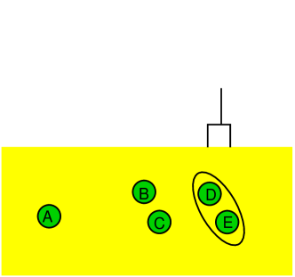
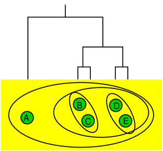
Figure 4: Example for agglomerative clustering: Initially one has a set of $n=5$ data points corresponding to $n$ clusters A, B, C, D, and E (bottom part). Iteratively the closest clusters are merged (illustrated by ellipses). For each merger, a branch in a dendrogram (tree) is generated (top part). Left: Situation after the first two single-point clusters D,E have been merged into a two-point cluster DE. Right: Final situation, after the merger of B with C, followed by the merger of BC with DE and finally the merger of A with BCDE. The dendrogram represents the hierarchical cluster structure.

The basic idea of agglomerative clustering is that one considers the initial set of $n$ data points as a set of $n$ clusters $C=\{c_{1},\ldots,c_{n}\}$ with $c_{i}=\{{\underline{x}}^{(i)}\}$. One defines cluster distances $d_{c}(i,j)$ between pairs of the initial clusters $c_{i}$ and $c_{j}$ as given by the selected point-to-point distance function $d(i,j)$, like the Euclidean distance Eq. (3) or any other suitable distance function. Within agglomerative clustering iteratively the two closest clusters $c_{i_{\min}}$ and $c_{j_{\min}}$, i.e., where

$$i_{\min},j_{\min}=\operatorname{argmin}_{i,j}d_{c}(i,j)\,,$$

are merged into one new single cluster $k=c_{i_{\min}}\cup c_{j_{\min}}$. Thus, within the first step, two clusters containing a single data point each will be merged. During the next steps, single-data point clusters or multiple-data point clusters will be merged. This is illustrated in Fig. 4. During each iteration the number of clusters will be decreased by one, hence, this process stops after $n-1$ iterations when all data points are collected in one single cluster. The merging process can be represented by a tree, called dendrogram: The leaves of the tree are given by the initial data points, i.e., the clusters $c_{1},\ldots,c_{n}$. Whenever two cluster are merged, a new (non-leaf) node is created, which has the two clusters as descendants. Therefore, the root of the tree is the node which has those two clusters as descendants, which were joined during the last iteration. Note when drawing the tree, it is convenient to order the leaves on the $x$-axis according to their appearance during a tree traversal, e.g. an inorder traversal, see Sec. 6.7 of Ref. [Hartmann (2015)].

The most important point is that when creating a cluster $c_{k}$ through a merger of $c_{i_{\min}}$ and $c_{j_{\min}}$, one has to provide new distances $d_{c}(k,l)$ of the new cluster $c_{k}$ to all other clusters $c_{l}$ with $l\neq i_{\min}$ and $l\neq j_{\min}$. Different approaches are possible. Here, we use the average-linking clustering, where the distance between two cluster $c_{k},c_{l}$ is the average distance of the data points in the two clusters:

$$d_{c}(k,l)=\frac{1}{|c_{k}||c_{l}|}\sum_{i\in c_{k},j\in c_{l}}d(i,j)\,,$$

where $|c_{k}|$ and $|c_{l}|$ represent the number of data points in the clusters $c_{k}$ and $c_{l}$, respectively. Thus, when cluster $c_{k}$ is created by merging $c_{i_{\min}}$ and $c_{j_{\min}}$, the distance of new cluster $c_{k}$ to all other clusters $c_{l}$ can be conveniently calculated via

$$d_{c}(k,l)=\frac{1}{|c_{k}|}\left\{|c_{i_{\min}}|d(i_{\min},l)+|c_{j_{\min}}|d(j_{\min},l)\right\}\,.$$

Many other choices for calculating cluster distances exists, basically they only have to have the property that the distances between clusters are monotonically increasing when merging. Common examples are taking the minimum or the maximum of the point-wise distances between the nodes of the cluster, specifying single-linkage and complete-linkage clustering. Another widely used method is Ward’s approach, where the geometric centers of the clusters are also taken into account. For details about many clustering algorithms see, e.g., Ref. [Jain and Dubes (1988)].

Once the clustering procedure is completed and the dendrogram calculated, the full clustering information is contained in the dendrogram, in particular the hierarchical structure, i.e., if clusters contain sub clusters that in turn contain sub clusters etc. To obtain a single set of clusters, a common approach is to use a threshold $\theta$ such that all inter-cluster distances are larger than $\theta$ and all intra-cluster distances are smaller or equal to $\theta$. This is similar to the neighbor-based clustering presented before, only that the intra-cluster distances for agglomerative clustering represent joint properties of sub clusters instead of single pairs of nodes. When drawing the dendrogram, one usually uses the $\delta=0$ (height) position for the leaves. For all other nodes, representing mergers of two clusters $i_{\min},j_{\min}$ , one uses a height $\delta\sim d_{c}(i_{\min},j_{\min})$, i.e., the distance of the two clusters which are merged. Thus, using a threshold $\theta$ corresponds to drawing a horizontal line at $\delta=\theta$ and cutting off all nodes above this line, c.f. Fig. 6. The remaining trees located below the line represent the clusters. Often a meaningful choice of $\theta$ is to cut the tree at a height value inside the largest interval where no node has its height in. This correspond to the iteration where the difference between the distances of the last and the current mergers is largest.

In the following, we discuss the C implementation of the single-linkage agglomerative clustering. First, we need a data structure for the nodes of the dendrogram. Each node stores the ID of the corresponding cluster and the size of the cluster. If the cluster was merged from two clusters, the node stores pointers (left and right) to nodes corresponding to these clusters as well as the distance of these two clusters, otherwise the corresponding entries are NULL (or 0). For this structure a new type name cluster_node_t is introduced:

typedef struct cluster_node
{
  int ID;                       /* ID of cluster */
  int size;                 /* number of members */
  double dist;       /* distance of sub clusters */
  struct cluster_node *left;      /* sub cluster */
  struct cluster_node *right;     /* sub cluster */
} cluster_node_t;

The function cluster_agglomerative() performs the actual clustering. It receives a matrix distance (GSL type gsl_matrix) of point-to-point distances, as calculated, e.g., by the function cluster_distances(). The function returns a pointer to the root of the dendrogram, which represents the clustering.

cluster_node_t *cluster_agglomerative(gsl_matrix *distance)
{
  cluster_node_t *tree;                      /* root of dendrogram */
  cluster_node_t *node;                     /* nodes of dendrogram */
  int num_points;              /* number of points to be clustered */
  int num_clusters;                  /* current number of clusters */
  int next_ID;                               /* ID of next cluster */
  int ID_curr;                            /* ID of current cluster */
  int ID_min1, ID_min2;     /* IDs of clusters having min distance */
  int last_ID;                 /* ID of cluster in last row/column */
  int entry_min1, entry_min2;        /* entry  having min distance */
  int c1, c2;                                     /* loop counters */
  int *pos;              /* position of cluster in distance matrix */
  int *cluster;  /* ID of cluster in each row/colum, inv. of ’pos’ */
  double delta;                              /* auxiliary distance */

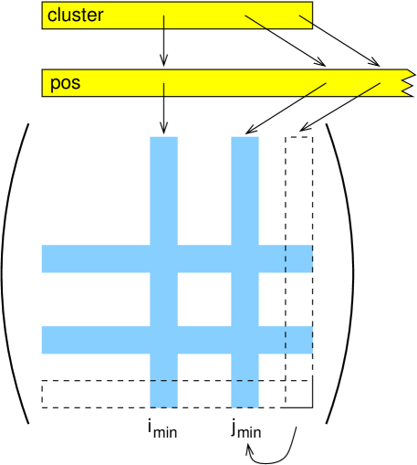
Figure 5: When merging clusters with IDs $i_{\min}$ and $j_{\min}$ ($i_{\min}<j_{\min}$), the distances of the new merged cluster are stored in the row and column where the distances of $i_{\min}$ were stored, while the entries corresponding to cluster with ID $j_{\min}$ are swapped with the last row and column. Top part: for each cluster, the current column and row is stored in the array pos, while for each column and row the current cluster is stored in the array cluster.

The distances among the data points as well as all cluster created during the process will be stored in the matrix distance. Since there are at most $n$ clusters existing at any time, the matrix distance is large enough. When two clusters are merged, the entries of one cluster will be used to store the distances of the merged cluster, while the entries of the other cluster will be disregarded; they will be exchanged with the distances stored in the last column and row. Thus, after a merger, the last column and row will not be used any more. In this way, the matrix distance is overwritten. The current number of used columns and rows, equal to the current number of clusters is stored in the variable num_clusters. Note that the cluster IDs are allocated in increasing manner, i.e., the IDs 0 to $n-1$ are for the single-data point clusters, the ID $n$ is for the first cluster created by a merger, the ID $n+1$ for the second, and so forth. Since the rows and columns of distance contain entries for all clusters, also for those which are created by mergers, i.e., with IDs larger than $n-1$, two additional arrays are used: The array pos stores for each cluster in which row and column the corresponding distances are stored currently. Inversely to pos, the array cluster stores for each row and column, which cluster is currently represented there. Thus, we have always pos[cluster[i]]==i and cluster[pos[i]]==i. The data arrangement is illustrated in Fig. 5.

In the C code, the number of data points is determined from the size of the matrix distance (line 16). Next, memory is allocated for the arrays cluster, pos and nodes (line 18–21). The latter two have $2n-1$ entries since this is the total number of clusters considered during the construction procedure. The initialization is completed by setting up the entries of pos and cluster and the nodes for the original data points (lines 23–32):

  num_points = distance->size1;

  cluster = (int *) malloc(num_points*sizeof(int));
  pos = (int *) malloc( (2*num_points-1)*sizeof(int));
  node = (cluster_node_t *)
         malloc( (2*num_points-1)*sizeof(cluster_node_t));

  for(c1=0; c1<num_points; c1++)                    /* initialize  */
  {
    pos[c1] = c1;
    cluster[c1] = c1;
    node[c1].left = NULL;
    node[c1].right = NULL;
    node[c1].dist = 0.0;
    node[c1].ID = c1;
    node[c1].size = 1;
  }

Initially, the number of clusters is equal to the number of data points $n$ (line 33) and the next available cluster ID will be $n$ (line 34). The main loop (lines 35–81) will be performed while there are clusters left for being merged. In the main loop, first the smallest current inter-cluster distance is determined (lines 37–44) and the corresponding clusters are obtained via the cluster array (lines 46,47):

  num_clusters = num_points;
  next_ID = num_clusters;
  while(num_clusters > 1)        /* until all clusters are merged */
  {
    entry_min1=0; entry_min2=1;  /* search min. off-diag distance */
    for(c1=0; c1<num_clusters; c1++)
      for(c2=c1+1; c2<num_clusters; c2++)
        if(gsl_matrix_get(distance, c1, c2) <
           gsl_matrix_get(distance, entry_min1, entry_min2))
        {
          entry_min1=c1, entry_min2=c2;
        }

    ID_min1 = cluster[entry_min1];       /* determine cluster IDs */
    ID_min2 = cluster[entry_min2];

Now, a new node can be set up. It contains pointers to its two sub clusters, its ID, its size which is the sum of the sizes of the two sub clusters, and the distance of the two sub clusters:

    node[next_ID].left = &(node[ID_min1]);      /* merge clusters */
    node[next_ID].right = &(node[ID_min2]);
    node[next_ID].ID = next_ID;
    node[next_ID].size = node[ID_min1].size + node[ID_min2].size;
    node[next_ID].dist =
      gsl_matrix_get(distance, entry_min1, entry_min2);

Next, the distances of the remaining clusters to the new clusters are calculated. These distances are stored in the entries of the first of the two merged clusters:

    for(c1=0; c1<num_clusters; c1++)  /* distances to new cluster */
      if(c1 == entry_min1)
        gsl_matrix_set(distance, entry_min1, c1, 0);
      else if(c1 != entry_min2)
      {
        ID_curr = cluster[c1];
        delta = node[ID_min1].size*
          gsl_matrix_get(distance, entry_min1, c1)+Ψ
          node[ID_min2].size*
          gsl_matrix_get(distance, entry_min2, c1);
        delta /= node[next_ID].size;
        gsl_matrix_set(distance, entry_min1, c1, delta);
        gsl_matrix_set(distance, c1, entry_min1, delta);
      }

Finally, the current number of clusters is reduced by one (line 68), the root of the dendrogram is set if necessary (lines 69 and 70) the entries of the last current row and column are put to the row and column where previously the distances of the second cluster were stored (lines 71–75), the entries of pos and cluster for the new cluster are set (lines 77 and 78), and the counter for the next available cluster ID is increased by one (line 79). After the main loop has finished, the memory which is associated to those data structures which are not used any more is freed (lines 83 and 84):

    num_clusters--;
    if(num_clusters == 1)
      tree = &(node[next_ID]);                /* set root of tree */
    last_ID = cluster[num_clusters];/* last cluster -> entry_min2 */
    pos[last_ID] = entry_min2;
    cluster[entry_min2] = last_ID;
    gsl_matrix_swap_rows(distance, num_clusters, entry_min2);
    gsl_matrix_swap_columns(distance, num_clusters, entry_min2);

    cluster[entry_min1] = next_ID;
    pos[next_ID] = entry_min1;
    next_ID++;
Ψ
  }

  free(pos);                                          /* clean up */
  free(cluster);

  return(tree);
}

Figure 6: Results of the clustering of sample set B with agglomerative clustering. Upper left: dendrogram using average linkage clustering for sample set A. Upper right: dendrogram using average linkage clustering for sample set B. Lower left: clusters for sample set B obtained when cutting the dendrogram at height $\delta=1.12$. Lower right: dendrogram using single-linkage clustering for sample set B.

In Fig. 6 the resulting dendrograms for sample sets A and B are shown. When cutting the dendrogram for sample set A at the most obvious height, indeed three clusters emerge. On the other hand, one has to cut the dendrogram for sample set B at a lower height to obtain a clustering where the cluster in the middle is separate from the “ring”, resulting in five clusters. When considering a height where four clusters emerge, the “central” cluster will be merged with the cluster to the left indicated by the symbol $\times$, thus “ring” and “central” part are not seperated. More successful is the single-linkage agglomerative approach (not shown here), but this is essentially equivalent to the neighbor-based clustering. The difference (and improvement) is that also a dendrogram is obtained which allows to obtain the most natural threshold and to analyze hierarchical sub structures.

Note that the source code file cluster.c also contains the function cluster_list_tree() which prints for a given dendrogram and a given threshold $\theta$ the positions of the data points ordered by the clusters, i.e., between every cluster there will be printed two empty lines. This function can be easily extended that, e.g., cluster IDs are assigned to the initial data points.

References

- [Bolobas (1998)] Bolobas, B. (1998). Modern Graph Theory, (Springer, New York).
-
[Galassi et al. (2006)]
Galassi M. et al (2006). GNU Scientific Library Reference Manual, (Network Theory Ltd, Bristol),
see also
http://www.gnu.org/software/gsl/. - [Hartmann (2015)] Hartmann, A. K. (2015), Big Practical Guide to Computer Simulations, (World-Scientific, Singapore)
- [Jain and Dubes (1988)] Jain, A. K. and Dubes R. C. (1988), Algorithms for Clustering Data, (Prentice-Hall, Englewood Cliffs, USA).
- [Swamy and Thulasiraman (1991)] Swamy, M. N. S. and Thulasiraman, K. (1991). Graphs, Networks and Algorithms, (Wiley, New York).