Suppression of collisionless magnetic reconnection in asymmetric current sheets

Abstract

Using fully kinetic simulations, we study the suppression of asymmetric reconnection in the limit where the diamagnetic drift speed $\gg$ Alfvén speed and the magnetic shear angle is moderate. We demonstrate that the slippage between electrons and the magnetic flux facilitates reconnection, and can even result in fast reconnection that lacks one of the outflow jets. Through comparing a case where the diamagnetic drift is supported by the temperature gradient with a companion case that has a density gradient instead, we identify a robust suppression mechanism. The drift of the x-line is slowed down locally by the asymmetric nature of the current sheet and the resulting tearing modes, then the x-line is run over and swallowed by the faster-moving following flux.

Introduction– The explosive release of magnetic energy through magnetic reconnection is ubiquitous in laboratory, space, and astrophysical plasmas Ji and Daughton (2011). The formation of a thin, kinetic-scale, current sheet is the requirement for fast reconnection Daughton et al. (2009); Cassak et al. (2005), but not all thin current sheets seemingly unstable to reconnection undergo reconnection. In a realistic situation, on both sides of the current sheet the pressures are not the same (i.e., asymmetric) and the magnetic fields are not anti-parallel (i.e., the magnetic shear angle $\phi\neq 180^{\circ}$), which induces the diamagnetic drifts of electrons and ions in the outflow direction of reconnection. It is a consensus that a strong drift may hinder magnetic reconnection Rogers and Zakharov (1995); Zakharov et al. (1993); Zakharov and Rogers (1992); Biskamp (1981); Grasso et al. (2012); Porcelli (1991); Galeev et al. (1985); Drake et al. (1983); Ara et al. (1978); Beidler and Cassak (2011); Swisdak et al. (2003). However, the fundamentals of how the suppression of reconnection occurs remains unclear, especially in collisionless plasmas.

The diamagnetic suppression of tearing modes (i.e., a linear mode that spontaneously leads to reconnection) Rogers and Zakharov (1995); Zakharov et al. (1993); Zakharov and Rogers (1992); Biskamp (1981); Grasso et al. (2012); Porcelli (1991); Galeev et al. (1985); Drake et al. (1983); Ara et al. (1978), among many other ideas, was extensively explored in order to model the sawtooth crashes that spoil the magnetic confinement in fusion devices von Goeler et al. (1974); Kadomtsev (1975). In particular, researchers want to explain why the reconnection associated with these crashes usually does not completely consume the available flux Soltwisch (1992); Levinton et al. (1994); Yamada et al. (1994) after an abrupt onset Zakharov and Rogers (1992); Wesson et al. (1991), which suggests a suppression of reconnection. The suppression is reflected in the reduction of the growth rate of tearing modes by the diamagnetic drift frequency, $\omega_{j}^{*}$. For instance, a suppression criterion $\omega_{j}^{*}>\gamma_{0}$ is observed through examining the saturation of magnetic islands in two-fluid models Rogers and Zakharov (1995); Biskamp (1981). Here $\gamma_{0}$ is the growth rate of tearing modes without the drift effect, and $j=i,e$ for ions and electrons respectively.

On the other hand, recent work examines the nonlinear development of reconnection Beidler and Cassak (2011); Swisdak et al. (2003) by comparing the diamagnetic drift speed, ${\bf U}^{*}_{j}=c{\bf B}\times\nabla{\bf P}_{j}/(nq_{j}B^{2})$, with the characteristic Alfvén speed, $V_{A}$, which is the typical reconnection outflow speed in non-drifting cases Petschek (1964). Swisdak et al. Swisdak et al. (2003) performed the first particle-in-cell (PIC) simulations to study this drift effect in collissionless reconnection. They observed that the x-line drifts with electrons at a speed $\sim U_{e}^{*}$. In this letter, velocity symbols in unbolded font are in the reconnection outflow direction (i.e., $\hat{x}$) unless otherwise specified. Due to the opposite sign of charges, ions drift against electrons and the x-line motion. This fact led them to hypothesize a suppression mechanism that is satisfied when the drift speed of ions in the x-line frame is larger than the Alfvén speed, i.e., $|U_{e}^{*}-U_{i}^{*}|>V_{A}$. In this scenario, they argued that one of the outflow jets can not develop, hence reconnection is suppressed. Swisdak’s criterion is widely used to interpret the occurrence distribution of reconnection at the magnetosphere of Earth Trenchi et al. (2015); Phan et al. (2013) and Saturn Fuselier et al. (2014); Masters et al. (2012), and in the solar wind Phan et al. (2010); Gosling and Phan (2013). However, recent gyro-kinetic simulations Kobayashi et al. (2014) were conducted to test this criterion in the low shear angle $\phi\ll 1$ (i.e., very strong guide field) and low plasma-$\beta$ ($\sim 0.1-0.01$) limit, and conclude that this suppression condition is not generally satisfied. In these simulations, the pressure gradient is decomposed into a combination of density and temperature gradients, $\nabla P_{j}=T_{j}\nabla n+n\nabla T_{j}$. The discrepancy was attributed to the coupling of reconnection with additional instabilities driven unstable by the density Rogers and Dorland (2005), electron temperature Kobayashi et al. (2014); Dorland et al. (2000) or ion temperature Connor and Wilson (1994) gradients.

In this letter, we describe in details the development and suppression of reconnection in the regime with a drift velocity $|U_{e}^{*}-U_{i}^{*}|\gg V_{A}$, and a moderate magnetic shear angle $\phi\sim 90^{\circ}$. This is the stable limit of Ref. Swisdak et al. (2003), and this limit requires the difference of plasma-$\beta$ on both sides of the current sheet to be large Swisdak et al. (2010), i.e., $\Delta\beta\gg 1$. In the two cases discussed, reconnection under a drift supported by $\nabla n$ is more or less suppressed, as expected, but reconnection persists under a drift supported by $\nabla T$. We find that the divergence of the full pressure tensor, $\nabla\cdot{\bf P}_{e}$, in the generalized Ohm’s law allows the slippage between the electrons and magnetic flux at the outflow region. This facilitates reconnection and even results in fast reconnection that lacks one of the outflow jets. Through comparing these two cases, we further demonstrate that the asymmetric nature of the current sheet in the $\nabla n$-case slows down the drift of the x-line, leading the following flux to run over and swallow the x-line. A lower bound for this new suppression mechanism is proposed, and it is different from that suggested in Ref. Swisdak et al. (2003) since the drift of ions are not required.

Table 1: Asymmetric feature of Runs

Case	$T_{1}$	$T_{2}$	$n_{1}$	$n_{2}$	$B_{1y}$	$B_{2y}$	$\rightarrow$ $\beta_{1}$	$\beta_{2}$	$|U_{e}^{*}-U_{i}^{*}|$
$\nabla T$	12.1	1.21	1	1	0.2	4.65	$\rightarrow$ 23	0.1	7
$\nabla n$	6.64	6.64	1.8	0.18	0.2	4.65	$\rightarrow$ 23	0.1	7

Simulation setup– Kinetic simulations were performed using the particle-in-cell code -VPIC (Bowers et al., 2009). The asymmetric configuration employed has the magnetic profile, ${\bf B}=B_{x^{\prime}}[0.5+\alpha_{1}\mbox{tanh}(z/\lambda)]\hat{\bf x}^{\prime}+B_{y^{\prime}}\hat{\bf y}^{\prime}$, density $n=\alpha_{3}[1-\alpha_{2}\mbox{tanh}(z/\lambda)]$, temperature $T=[\alpha_{4}-B_{x}^{2}/2]/n$ to satisfy the force balance. The pressure gradient is the same for the two cases considered here and the $\nabla T$ ($\nabla n$)-case has an asymmetric temperature (density) profile in the z-direction. We initialize $B_{y^{\prime}}=0.22B_{x^{\prime}}$, $\alpha_{1}=0.55$, $\alpha_{3}=0.55$ and $\alpha_{4}=0.37$. We use $\alpha_{2}=0.82$ for the $\nabla n$-case and $\alpha_{2}=0$ for the $\nabla T$-case. To make a better comparison with the runs in Ref. Swisdak et al. (2003), the 2D simulation plane is then rotated (with respect to the z-axis) to the plane where the reconnecting components are equal, $|B_{1x}|=|B_{2x}|=B_{0}$. Here the subscripts “2” and “1” indicate the side at $z>0$ and $z<0$ respectively. The resulting asymmetries are summarized in Table I. The magnetic fields are normalized to the reconnecting field $B_{0}$ and the guide field strength at the location of $B_{x}=0$ is $\sim 2$. Densities are normalized to $n_{0}$. Spatial scales are normalized to the ion inertial length $d_{i}\equiv c/\omega_{pi}$, where the ion plasma frequency $\omega_{pi}\equiv(4\pi n_{0}e^{2}/m_{i})^{1/2}$. Time scales are normalized to the ion gyro-frequency $\Omega_{ci}\equiv eB_{0}/m_{i}c$. For these two cases, the effective Alfvén speeds Swisdak and Drake (2007) $V^{2}_{A}=(|B_{1x}|+|B_{2x}|)/[4\pi m_{i}\left(n_{1}/|B_{1x}|+n_{2}/|B_{2x}|)\right]$ are designed to be the same. This $V_{A}=d_{i}\Omega_{ci}$ hence will be used to normalize velocities. The temperature is normalized by $m_{i}V_{A}^{2}$. The initial thickness of the current sheet $\lambda=0.37d_{i}$, the temperature ratio is $T_{i}/T_{e}=2$, the mass ratio is $m_{i}/m_{e}=200$, the ratio of electron plasma to gyro-frequency is $\omega_{pe}/\Omega_{ce}=4.17$, and the total magnetic shear angle $\phi=\mbox{tan}^{-1}(B_{0}/B_{1y})+\mbox{tan}^{-1}(B_{0}/B_{2y})\approx 90.8^{\circ}$. The system size is $76d_{i}\times 19d_{i}$ with grids $8192\times 4096$ for the $\nabla T$-case and $4096\times 2048$ for the $\nabla n$-case. The resolution of the $\nabla T$-case is higher in order to reduce the noise in the calculation of the generalized Ohm’s law presented here. The boundary conditions are periodic in the x direction, while the z direction is conducting for fields and reflecting for particles. We use a localized perturbation to induce a single x-line at $x=0$. Both cases have an initial peak $|U^{*}_{i}-U^{*}_{e}|/V_{A}\approx 7$ and $\Delta\beta\equiv|\beta_{1}-\beta_{2}|\approx 23$.

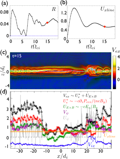
Figure 1: Features of the $\nabla T$-case. In (a), the normalized reconnection rate, $R$. In (b), the drift velocity of the primary x-line, $U_{xline}$. In (c), the x-component of electron velocity with the in-plane magnetic flux overlaid at time $15/\Omega_{ci}$. In (d), the $V_{ex}$, $V_{ix}$, $U_{e}^{*}$, $U_{{\bf E}\times{\bf B}}$, $V_{\psi}$ and $U_{\psi}$ along the trajectory where $B_{x}=0$ (indicated as the light blue curve in (c)). The approximation of $V_{ex}$, $U_{e}^{*}$ and $U_{{\bf E}\times{\bf B}}$ are plotted as asterisks. The $U_{xline}$ is plotted as a horizontal line for reference.

$\nabla T$ case– Contrary to the heuristic prediction proposed in Ref. Swisdak et al. (2003), reconnection proceeds under such a high $|U_{e}^{*}-U_{i}^{*}|/V_{A}$. A reconnection rate $R\sim 0.05$ is sustained, and the x-line drifts in a rather steady velocity $U_{xline}\sim 0.5V_{A}$ as shown in Fig. 1(a)-(b). Here $R\equiv\left<\partial\Delta\psi/\partial t\right>/(B_{0}V_{A})$ with $\Delta\psi\equiv\mbox{max}(\psi)-\mbox{min}(\psi)$ along the $B_{x}=0$ trajectory and $\psi$ is the in-plane magnetic flux. The $V_{ex}$ at time $15/\Omega_{ci}$ overlaid with the contour of $\psi$ is shown in (c). We can understand the composition of $V_{ex}$ from the momentum equation $m_{e}nd{\bf V}_{e}/dt=-en({\bf E}+{\bf V}_{e}\times{\bf B}/c)-\nabla\cdot{\bf P}_{e}$. We consider a subsonic regime where the $d{\bf V}_{e}/dt$ term is negligible (Goldston and Rutherford, 1995). By curling the rest of this equation with ${\bf B}$ leads to $-en[{\bf E}\times{\bf B}-{\bf V}_{e}B^{2}/c+{\bf B}({\bf V}_{e}\cdot{\bf B})/c]-\nabla\cdot{\bf P}_{e}\times{\bf B}=0$, which shows that the perpendicular flow is the combination of the ${\bf E}\times{\bf B}$ drift and diamagnetic drift: ${\bf V}_{e\perp}\approx c{\bf E}\times{\bf B}/B^{2}-c{\bf B}\times\nabla\cdot{\bf P}_{e}/(enB^{2})$.

We plot the x-component of electron drifts along the $B_{x}=0$ trajectory in Fig. 1(d). These velocities along this trajectory are perpendicular to the local magnetic field, hence are relevant to the transport of magnetic structures inside the current sheet. To good approximation, with $B_{x}=0$

$$V_{ex}={V}_{e\perp,x}\approx-\frac{cE_{z}}{B_{y}}-\frac{c\partial_{z}P_{ezz}}{neB_{y}}.$$ (1)

These approximations are verified by the fact that those asterisks closely trace the solid curves in Fig. 1(d). The $E_{z}$ associated with the $U_{{\bf E}\times{\bf B}}$ develops in our simulations within time $1/\Omega_{ci}$ partially because the current sheet relaxes into a kinetic equilibrium. Note that, although the local drift speed near the x-line drops to a steady value $V_{ex}\sim V_{A}$ during the nonlinear evolution, reconnection proceeds with a higher $V_{ex}\gtrsim 3V_{A}$ in the earlier stage. (e.g., also the tearing modes at $x<-15d_{i}$ in Fig. 1(c)).

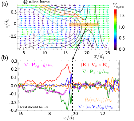
Figure 2: A blow up of the drift x-line in Fig. 1. In (a), the electron flow and the in-plane flux are shown in the x-line drift frame. Here $|V_{e,xz}|\equiv(V_{ex}^{2}+V_{ez}^{2})^{1/2}$. In (b), terms of the generalized Ohm’s law are evaluated along the orange line at a fixed z indicated in (a).

We zoom in on the region around the x-line in Fig. 2 (a). The electron flow pattern is shown in the x-line drift frame. Unlike the typical flow pattern around an x-line, the electrons are not repelled leftward of the x-line to form a jet. A similar observation applies for the ions, since $V_{ix}<U_{xline}$ persists inside the current sheet as indicated in Fig. 1(d). Surprisingly, reconnection remains fast with only one jet. However, the reconnected magnetic flux needs to leave the x-line to both sides, regardless of the magnitude of transport speed. Fig. 2(b) shows a finite value of the y-component of the non-ideal electric field (red) at the left side of the x-line, which indicates the slippage between electrons and flux. Hence the flux can propagate out of the x-line while the electrons flow in. This is reflected in the fact that the observed flux advection velocity, $V_{\psi}$, is smaller than $U_{xline}$ at the left side of the x-line (i.e., between $x\sim 5$ to $15d_{i}$) in Fig. 1(d). The $\nabla\cdot{\bf P}_{e}$ term (green) contributes to this non-ideal electric field and hence enables this slippage. We approximate the full pressure tensor in a gyrotropic form ${\bf P}_{eg}\equiv P_{e\perp}{\bf I}+(P_{e\|}-P_{e\perp}){\bf bb}$, where ${\bf b}\equiv{\bf B}/|B|$, the parallel pressure $P_{e\|}\equiv{\bf b}\cdot{\bf P}_{e}\cdot{\bf b}$ and the perpendicular pressure $P_{e\perp}\equiv[\mbox{Tr}({\bf P}_{e})-P_{e\|}]/2$. Then $\nabla\cdot{\bf P}_{eg}\cdot\hat{y}=\nabla\cdot(P_{e\|}-P_{e\perp}){\bf b}\mbox{b}_{y}$. The evaluation of this term (pink) suggests that the pressure anisotropy contributes significantly to this slippage, while the difference between $\nabla\cdot{\bf P}_{e}\cdot\hat{y}$ and $\nabla\cdot{\bf P}_{eg}\cdot\hat{y}$ closer to the x-line is attributed to the nongyrotropy Aunai et al. (2013); Hesse et al. (2011).

In addition, we can estimate the advection speed of the in-plane flux. In 2D, we can write ${\bf B}=\hat{y}\times\nabla\psi+B_{y}\hat{y}$. By performing $\hat{y}\times[\partial_{t}{\bf B}+c\nabla\times{\bf E}=0]$ gives $E_{y}=(1/c)\partial_{t}\psi$. This leads the y-component of the electron force balance, $\hat{y}\cdot[{\bf E}+{\bf V}_{e}\times{\bf B}/c=-(1/en)\nabla\cdot{\bf P}_{e}]$, at where $B_{x}=0$ into an advection equation, $\partial_{t}\psi+U_{\psi}\partial_{x}\psi=0$. The estimated advection velocity of $\psi$ is

$$U_{\psi}=V_{ex}-\frac{c\nabla\cdot{\bf P}_{e}\cdot\hat{y}}{enB_{z}}.$$ (2)

This expression is valid at the region where $B_{z}\neq 0$. This also excludes the singular x-line where $\psi$ is generated and the $\nabla\cdot{\bf P}_{e}$ term should be treated as a source term. This $U_{\psi}$ in Fig. 1(d), although noisy, follows well with the measured $V_{\psi}$. In this case $U_{\psi}$ and $V_{\psi}$ do not match well with $V_{ex}$, which again implies a significant slippage that facilitates reconnection.

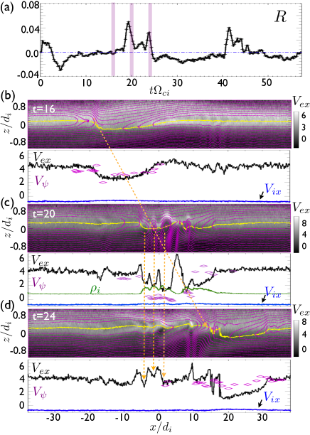
Figure 3: The long term evolution of the $\nabla n$-case. In (a), the normalized reconnection rate, $R$. Panels (b), (c) and (d) show the $V_{ex}$ map overlaid with the in-plane flux at times marked in (a). The $V_{ex}$, $V_{ix}$ and $V_{\psi}$ along the trajectory where $B_{x}=0$ (the yellow curves in the 2D map) are plotted underneath each panel. The ion gyro-radius, $\rho_{i}$, is also shown in (c). The oblique yellow dashed line tracks the motion of the following flux, while the three nearly vertical yellow dashed lines track the motion of tearing modes and active x-lines therein.

$\nabla n$ case– On the other hand, the suppression becomes pronounced in the $\nabla n$-case. For the simulations presented here, the induced x-line does not reconnect. However, over longer times tearing modes are triggered and then suppressed, resulting in a periodic burst of reconnection as shown in Fig. 3(a). This cyclic behavior reveals the nature of suppression.

Fig. 3(b)-(d) show the contours of $\psi$ and $V_{ex}$ around the period of the first burst of reconnection at time 16, 20 and $24/\Omega_{ci}$. The induced x-line remains inactive in (b). The tearing modes with a significant growth are triggered at the trailing edge of the primary island in (c), which boost the reconnection rate up to $\sim 0.05$. In (d), these tearing islands do not propagate and hence are run over and swallowed by the following flux that maintains a steady positive velocity $\sim 4V_{A}$. This motion completely shuts off the reconnection. The tendency is also reflected in the the profile of $V_{\psi}$ (purple), which follows the trend of $V_{ex}$. Due to the asymmetric nature of the current sheet, a trough in the $V_{\psi}$ profile develops with the x-line sitting at the bottom as shown in Fig. 3(b). The negative slope at the left side of the x-line indicates this tendency of running-over. The birth of tearing modes further diverts the electron flow to the upper side of tearing islands, and this only deepens the $V_{\psi}$ trough in (c), which eventually results in the running-over in (d). The same reason explains why tearing modes only become feasible temporarily at the edge where the $V_{\psi}$ profile has a positive slope, which delays the running-over. In contrast, for the $\nabla T$-case shown in Fig. 1(c), the current sheet and the resulting tearing modes are more or less symmetric. Hence the tearing islands and the induced x-line can pick up the peak drift velocity available to advect flux. The in-plane magnetic structures in the $\nabla T$-case all propagate in a positive velocity $\sim V_{A}$ as indicated by the $V_{\psi}$ in Fig. 1(d). These x-lines will not be run over by the following flux and reconnection persists. As opposed to the asymmetric feature of tearing modes, a potential magnetization of the ions does not cause the local reduction of $V_{\psi}$ in the $\nabla n$-case, since the local ion gyro-radius ($\sim d_{i}$) does not decrease at the tearing islands and the ion drift $V_{ix}$ is barely affected as shown in Fig. 3(c). These observations suggest that this suppression mechanism does not require the drift of ions, and hence differs from that proposed in Ref. Swisdak et al. (2003). It is also interesting to point out that the burst of fast reconnection can last longer if tearing modes grow faster and form a spatially longer tearing-mode-chain, so that the following flux needs more time to swallow them one-by-one. This phenomenon is seen in a companion case with hotter electrons (e.g., a case with $T_{i}/T_{e}=0.3$, not shown).

Figure 4: The velocity profiles around the x-line in the x-line drift frame. Here the x-line is at $x=0$ and the slippage is assumed negligible. In (a), $\Delta U^{*}_{e}>V_{A}$. In (b), $\Delta U^{*}_{e}<V_{A}$.

Model– To model the lower bound for this suppression, we consider an ideal situation without slippage, i.e., $V_{\psi}\approx V_{ex}\approx U_{e}^{*}+U_{{\bf E}\times{\bf B}}$. The asymmetric nature of the current sheets causes a trough in the profile of $U_{e}^{*}$ locally near the x-line, while the magnetic tension force in $d_{i}$-scale tends to drive electrons to the Alfvén speed $V_{A}$ outwardly from the x-line Rogers et al. (2001), and this effect enters the $U_{{\bf E}\times{\bf B}}$ drift. Fig. 4(a) shows a case where the depth of the trough, $\Delta U^{*}_{e}$, is larger than the asymptotic value of $|U_{{\bf E}\times{\bf B}}|\sim V_{A}$. Note that, these velocities are measured in the x-line drift frame. The resulting $V_{\psi}$ has a trough with a negative slope at the left side of the x-line, hence the x-line will be run over. If $\Delta U^{*}_{e}<V_{A}$ as in (b), the $V_{\psi}$ profile only has a positive slope and is free from this suppression mechanism. The $\nabla n$-case falls into the category of Fig. 4(a). The $\nabla T$-case falls into the category of (b) after accounting for the slippage. Based on these observations, we conclude that the suppression of reconnection, a least, requires $\Delta U^{*}_{e}>V_{A}$.

Summary and Discussion– A new suppression mechanism cased by the local reduction of flux transport speed is identified inside the ion diffusion region. This robust mechanism can completely shut off reconnection after a rapid onset. The magnitude of $\Delta U^{*}_{e}$ is determined by the asymmetric nature of the current sheet and the resulting tearing modes. For the $\nabla n$-case, the asymmetric nature may come from the mismatch between the x-line and the flow stagnation point (i.e., $\delta_{x2}/\delta_{x1}=B_{2}/B_{1}$ and $\delta_{s2}/\delta_{s1}=n_{2}B_{1}/n_{1}B_{2}$ in Ref. Cassak and Shay (2007)), which does not develop with only the asymmetry in temperature, as the $\nabla T$-case. In the limit of strong density asymmetry, the tearing modes and active x-lines therein barely drift as in the $\nabla n$-case presented here, then the $\Delta U^{*}_{e}$ is similar to the equilibrium $U_{e}^{*}$ of the current sheet. The lower bound for this suppression reduces to a simpler form $U_{e}^{*}>V_{A}$.

This study also shows that reconnection with only one jet in the x-line drift frame is possible due to the slippage between plasmas and the magnetic flux. This fact suggests the need for improving the identification of reconnection events at Earth’s magnetopause, and this could be studied using NASA’s on-going Magnetospheric Multiscale mission that is capable of evaluating $\nabla\cdot{\bf P}_{e}$ routinely.