Critical relaxation with overdamped quasiparticles in open quantum systems

Abstract

We study the late-time relaxation following a quench in a open quantum many-body system. We consider the open Dicke model, describing the infinite-range interactions between $N$ atoms and a single, lossy electromagnetic mode. We show that the dynamical phase transition at a critical atom-light coupling is characterized by the interplay between reservoir-driven and intrinsic relaxation processes in absence of number conservation. Above the critical coupling, small fluctuations in the occupation of the dominant quasiparticle-mode start to grow in time while the quasiparticle lifetime remains finite due to losses. Near the critical interaction strength we observe a crossover between exponential and power-law $1/\tau$ relaxation, the latter driven by collisions between quasiparticles. For a quench exactly to the critical coupling, the power-law relaxation extends to infinite times, but the finite lifetime of quasiparticles prevents ageing to appear in two-times response and correlation functions. We predict our results to be accessible to quench experiments with ultracold bosons in optical resonators.

In a closed system, the relaxation toward the equilibrium state is governed by processes which break integrability, allowing for an efficient redistribution of energy and momentum between the degrees of freedom. In this respect, important differences arise between classical and quantum systems Polkovnikov et al. (2011); Eisert et al. (2015). By contrast, in an open system the relaxation toward equilibrium is driven by exchange of energy and momentum with an external reservoir, so that the integrability-breaking intrinsic to the system does not necessarily play a role in the late-time dynamics close to the stationary state. In driven, dissipative systems, the latter is also generically different from a thermal-equilibrium state, since detailed balance is usually violated. Moreover, the presence of quantum correlations allows for the existence of entangled stationary pure states determined by the reservoir Diehl et al. (2008). The scenario becomes even richer if one considers the relaxation dynamics close to a phase transition. Already for classical systems the standard theory of critical dynamics near equilibrium phase transitions Hohenberg and Halperin (1977) does not fully characterize the relaxation after quenches, since ageing-like behavior violates detailed-balance Calabrese and Gambassi (2005). The extension of these concepts to quantum and open systems constitutes a challenging task which has recently received much attention both for the near-steady-state Mitra et al. (2006); Patanè et al. (2008); Diehl et al. (2010); Dalla Torre et al. (2010); Klaers et al. (2010); Kessler et al. (2012); Kirton and Keeling (2013); Sieberer et al. (2013); Täuber and Diehl (2014); Bonnes et al. (2014); Marcuzzi et al. (2014); Hoening et al. (2014); Medvedyeva et al. (2015); Labouvie et al. (2015); Maghrebi and Gorshkov (2015); Marino and Diehl (2016) and quench Marino and Silva (2012); Sedlmayr et al. (2013); Cai and Barthel (2013); Horstmann et al. (2013); Foss-Feig et al. (2013); Gagel et al. (2014); Piazza and Strack (2014); Schütz and Morigi (2014); Schütz et al. (2015); Sciolla et al. (2015); Buchhold and Diehl (2015) dynamics, also due to remarkable experimental advances in the control of hybrid systems involving phonons/photons coupled to ions Blatt and Roos (2012); Britton et al. (2012), excitons Carusotto and Ciuti (2013), superconducting circuits Hartmann et al. (2008); Houck et al. (2012); Schmidt and Koch (2013), mechanical modes Ludwig and Marquardt (2013), or neutral atoms Vetsch et al. (2010); Ritsch et al. (2013); Goban et al. (2014); Douglas et al. (2015).

In this work, we consider an open quantum many-body system close to a phase transition, where the interplay between dissipation and integrability breaking in absence of number conservation gives rise to a novel scenario for the post-quench relaxation dynamics. We consider an open version Dimer et al. (2007); Keeling et al. (2010); Bhaseen et al. (2012); Öztop et al. (2012); Kónya et al. (2012); Nagy et al. (2011); Torre et al. (2013); Tomka et al. (2013); Genway et al. (2014); Nagy and Domokos (2015); Acevedo et al. (2015) of the paradigmatic Dicke model Dicke (1954), describing $N$ two-level atoms equally coupled to a single, lossy mode of the electromagnetic field Hepp and Lieb (1973); Wang and Hioe (1973); Lambert et al. (2004); Vidal and Dusuel (2006); Liu et al. (2009); Larson and Lewenstein (2009); Nagy et al. (2010); Mumford et al. (2014), recently realized experimentally with atoms in optical cavities Baumann et al. (2010, 2011); Brennecke et al. (2013); Ritsch et al. (2013); Baden et al. (2014); Keßler et al. (2014); Klinder et al. (2015). Due to the infinite range of the atom-photon interactions ($0$-dimensionality), this model is integrable in the thermodynamic limit: $N=\infty$, corresponding to non-interacting polaritonic quasiparticles. Despite the absence of local degrees of freedom (typically used to characterize equilibration Fagotti and Essler (2013)), integrability breaking in the Dicke model at finite $N$ has been shown to lead to chaotic behavior Emary and Brandes (2003); Bakemeier et al. (2013) and thermalization Altland and Haake (2012) in the closed-system case. Thermalization can also be achieved at $N=\infty$ via disorder Buchhold et al. (2013). Here we describe the late-time dynamics following a quench of the atom-light coupling strength in the open system at finite $N$. We show that quantum non-equilibrium fluctuations induced by quasiparticle interactions trigger a dynamical phase transition, which causes the occupation of the dominant quasiparticle-mode to become unstable and grow in time. However, the quasiparticle lifetime remains finite in presence of the Markovian losses. In the critical regime, we predict a crossover between exponential and power-law $1/\tau$ relaxation. The latter is driven by quasiparticle collisions and extends to infinite times for a quench exactly to the critical point. However, since the quasiparticles involved retain a finite lifetime throughout the transition, the equilibration time does not diverge, thus ageing is not observed in two-times functions.

The algebraic dynamics with overdamped quasiparticles is a genuine out-of-equilibrium many-body effect, not related to critical slowing down since the system size $N$ is finite. The description of the relaxation driven by quasiparticles collisions requires non-perturbative many-body techniques. In particular, it cannot be described using mean-field approaches.

Quench experiments performed recently in the open Dicke model Klinder et al. (2015) have started exploring the dynamical phase transition, for which our theory provides the quantum description of the critical relaxation. Our predictions will be observable in the late-time behavior of response and correlation functions after small quenches near the critical point.

I The model

The Dicke model Dicke (1954) describes the coupling of $N$ two-level atoms to a single mode of the electromagnetic field with the Hamiltonian

$$\hat{H}=\omega_{0}\hat{a}^{\dagger}\hat{a}+\omega_{z}\hat{S}_{z}+\frac{2g}{\sqrt{N}}\hat{S}_{x}\left(\hat{a}^{\dagger}+\hat{a}\right).$$ (1)

Here $\hat{S}_{z,x}=\frac{1}{2}\sum_{i=1}^{N}\sigma_{i}^{z,x}$ are collective spin operators with the single-atom Pauli matrices $\sigma_{i}^{z,x}$ and $\hat{a}^{\dagger}$ and $\hat{a}$ are the bosonic photon creation and annihilation operators. $\omega_{0}$ is the characteristic photon frequency, $\omega_{z}$ the splitting of the atomic levels and $g$ is the photon-atom coupling strength. We will consider an open version of this model by introducing Markovian photon losses with a rate $\kappa$. The non-unitary time evolution is described by the master equation for the density matrix $\rho$,

$$\partial_{t}\rho=-i\left[\hat{H},\rho\right]+\kappa\left(2\hat{a}\rho\hat{a}^{\dagger}-\left\{\hat{a}^{\dagger}\hat{a},\rho\right\}\right).$$ (2)

Since we will be interested in large atom numbers $N$, we perform a Holstein-Primakoff transformation: $S_{z}=-N/2+\hat{b}^{\dagger}\hat{b}$ and $S^{+}=\hat{b}^{\dagger}\sqrt{N-\hat{n}}\approx\sqrt{N}\hat{b}^{\dagger}\left(1-\hat{n}/(2N)\right)$, while $S_{x}=\frac{1}{2}\left(S^{+}+S^{-}\right)$ and $S^{-}={S^{+}}^{\dagger}$, yielding the following Hamiltonian

$$\begin{split}\hat{H}&=\hat{H}_{0}+\hat{H}^{\prime}\\ \hat{H}_{0}&=\omega_{0}\hat{a}^{\dagger}\hat{a}+\omega_{z}\hat{b}^{\dagger}\hat{b}+g\left(\hat{a}+\hat{a}^{\dagger}\right)\left(\hat{b}+\hat{b}^{\dagger}\right)\\ \hat{H}^{\prime}&=-\frac{g}{2N}\left(\hat{a}+\hat{a}^{\dagger}\right)\left(\hat{b}^{\dagger}\hat{b}^{\dagger}\hat{b}+\hat{b}^{\dagger}\hat{b}\hat{b}\right)+\text{O}\left(\frac{1}{N^{2}}\right).\end{split}$$ (3)

For $N=\infty$ the interaction Hamiltonian $\hat{H}^{\prime}$ vanishes and the model is integrable i.e. describes non-interacting quasiparticles corresponding to polaritonic collective modes mixing atomic and photonic excitations. This quadratic model has a superradiant transition Hepp and Lieb (1973); Wang and Hioe (1973) at a critical coupling strength Dimer et al. (2007); Kónya et al. (2012); Nagy et al. (2011); Öztop et al. (2012)

$$g_{c,0}=\sqrt{(\omega_{0}^{2}+\kappa^{2})\omega_{z}/(4\omega_{0})},$$ (4)

where a finite average polarization $\langle\hat{b}\rangle\propto\sqrt{N}$ and a finite coherent light component $\langle\hat{a}\rangle\propto\sqrt{N}$ spontaneously break the $\mathbb{Z}_{2}$ symmetry. The transition is caused by a soft mode (see also Fig. 1) with zero characteristic frequency $\omega_{\rm qp}$, which switches from being damped to growing in time, i.e. the damping rate $\kappa_{\rm qp}$ crosses zero at $g_{c,0}$. The transition is purely dissipative, i.e. characterized by completely overdamped quasiparticles $\kappa_{\rm qp}\geq 0$ and $\omega_{\rm qp}=0$. This is due to the presence of Markovian losses while the transition is driven by the Hamiltonian sector Torre et al. (2013).

The Hamiltonian (3) does not conserve the excitation-number since it contains counter-rotating terms. This has the same effect as a driving term, which can indeed compensate the effect of losses, resulting in a steady state with a finite excitation number Dimer et al. (2007); Bhaseen et al. (2012); Öztop et al. (2012); Torre et al. (2013). Moreover, as it is the case in driven-dissipative systems, the coexistence of counter-rotating terms and Markov losses violates the detailed balance characterizing global equilibrium (see Torre et al. (2013) and Section III).

We conclude this section by pointing out that the absence of a continuum (or extensive number) of degrees of freedom does not prevent the system to show many-body behavior. The Dicke model, due to the infinite range of atom-light interactions, is 0-dimensional i.e. the spatial structure is lost. It therefore describes many quasiparticle excitations occupying the 4 possible polaritonic collective modes. The non-integrable model $N<\infty$ includes interactions between these quasiparticles. Given the unlimited Hilbert space in every mode and since the occupation numbers are generically large ($O(N^{1/2})$) in the scaling regime, see Torre et al. (2013) and Section III), there is no notion by which the system describes a few-body or impurity problem. In particular, for the critical late-time dynamics of the system the relaxation i.e. redistribution of energy between the modes is strongly affected by quasiparticle collisions. This behavior cannot be described using mean-field approaches and rather requires many-body techniques as the non-perturbative diagrammatics introduced next.

II Approach

The non-equilibrium critical properties of the open Dicke model have been recently investigated in near-steady-state Brennecke et al. (2013); Kulkarni et al. (2013); Kónya et al. (2014) and quench Klinder et al. (2015); Bhaseen et al. (2012) experiments. Here we want to go beyond the semiclassical studies and describe the critical post-quench late-time relaxation including quantum fluctuations due to quasiparticle interactions at finite system sizes as well as classical fluctuations from the Markov reservoir. We adopt a diagrammatic technique based on the real-time Keldysh functional-integral formulation of the Dyson equation Kamenev (2011); Sieberer et al. (2015), extending the steady state approach developed in Torre et al. (2013) to include the relaxation induced by quasiparticle collisions as well as the breaking of time-translation invariance. In the Keldysh functional-integral approach , one derives the two coupled Dyson equations for the retarded and Keldysh Green’s function (GF):

$$G^{K}=G^{R}\circ\left(\Sigma^{K}-D_{0}^{K}\right)\circ G^{R^{\dagger}}$$ (5)

$$\left(\left[G^{R}_{0}\right]^{-1}-\Sigma^{R}\right)\circ G^{R}=\delta(t-t^{\prime}),$$ (6)

where “$\circ$” indicates the convolution in real time. Due to the absence of number conservation in the Hamiltonian, the GFs are 4 by 4 matrices: $i\left(G^{K}(t,t^{\prime})\right)_{\rm i,j}=\langle\{\hat{V}_{\rm i}(t),\hat{V}_{\rm j}^{\dagger}(t^{\prime})\}\rangle$ and $i\left(G^{R}(t,t^{\prime})\right)_{\rm i,j}=\theta(t-t^{\prime})\langle[\hat{V}_{\rm i}(t),\hat{V}_{\rm j}^{\dagger}(t^{\prime})]\rangle$, with $\hat{V}^{T}=(\hat{a},\hat{a}^{\dagger},\hat{b},\hat{b}^{\dagger})$.

The retarded GF encodes the spectral response of the system, the Keldysh GF its correlation functions. As detailed-balance cannot be assumed, we must determine $G^{R}$ and $G^{K}$ independently through Eqs. (5),(6). The retarded GF $G_{0}^{R}$ and the matrix $D_{0}^{K}$ are fixed by the non-interacting theory $\hat{H}^{\prime}=0$ and given in the Appendix A. Finally, the self-energies $\Sigma^{(K,R)}=\Sigma^{(K,R)}\!\!\left[G^{R},G^{K}\right]$ are computed within a self-consistent Hartree-Fock (SCHF) approximation (as for instance employed to describe spin-chain dynamics Marcuzzi et al. (2013)), corresponding to the selection of Feynman diagrams shown in Fig. 4. Self-consistency is necessary to treat late-time relaxation close to the steady state Kamenev (2011). This is true despite the presence of the Markov reservoir since the system is close to a phase transition. Moreover, the inclusion of the Fock processes we perform here is required to describe the effect of quasiparticle collisions on the late-time relaxation of the system after a quench.

III Results

Starting from an initial atom-photon coupling $g_{i}$, we consider a sudden quench to a value $g>g_{i}$. We solve the coupled Dyson Eqs. (5),(6) in the SCHF approximation in the limit of large absolute times $\tau=(t+t^{\prime})/2$, i.e. for small relative deviations from the steady state, by means of an iterative numerical procedure. This approximate time-evolution is illustrated in detail in the Appendix B. In the limit of relative times $t_{\rm rel}$ long compared to the quasiparticle lifetime $1/\kappa_{\text{qp}}$, that is, including only the dominant contribution from low-frequency quasiparticles, the solutions take the following form

$$\left(G^{K}(t_{\text{rel}},\tau)\right)_{\rm i,j}\simeq e^{-\kappa_{\text{qp}}|t_{\text{rel}}|}$$

$$\times\left(G^{K}(0,\infty)+\frac{\delta G^{K}(0,0)}{e^{\kappa_{\text{kin}}\tau}+\frac{\lambda_{\text{kin}}}{\kappa_{\text{kin}}}\delta G^{K}(0,0)\left(e^{\kappa_{\text{kin}}\tau}-1\right)}\right),$$

$$\left(G^{R}(t_{\text{rel}},\tau)\right)_{\rm i,j}\simeq\theta\left(t_{\text{rel}}\right)e^{-\kappa_{\text{qp}}t_{\text{rel}}}$$

$$\times\left(G^{R}(0,\infty)+\frac{\delta G^{R}(0,0)}{e^{\kappa_{\text{kin}}\tau}+\frac{\lambda_{\text{kin}}}{\kappa_{\text{kin}}}\delta G^{K}(0,0)\left(e^{\kappa_{\text{kin}}\tau}-1\right)}\right),$$ (7)

where we used the notation $\delta G^{R/K}(0,0)=G^{R/K}(0,0)-G^{R/K}(0,\infty)$.

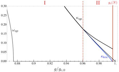
Figure 1: Qualitative behavior of the quasiparticle characteristic frequency $\omega_{\rm qp}$ (gray) and inverse lifetime $\kappa_{\rm qp}$ (black), together with the system’s damping rate $\kappa_{\rm kin}$ (blue), as a function of the final value $g$ of the light-matter coupling after a sudden quench from $g_{i}<g$. The dashed line corresponds to the prediction of the non-interacting theory $\hat{H}^{\prime}=0$, where $\kappa_{\rm kin}=\kappa_{\rm qp}$. For $\omega_{\rm qp}$ there is no difference between interacting and non-interacting predictions at large enough $N$.

Every component ${\rm i,j}=1,...,4$ of both retarded and Keldysh GFs follows the functional form (III) since the latter is determined by the least-damped quasiparticle mode corresponding to the dominant eigenvector of the 4 by 4 matrices . The solutions depend only on three parameters whose behavior is shown in Fig. 1 and 2 as a function of the coupling strength $g$: the quasiparticle inverse lifetime $\kappa_{\rm qp}$ (damping the relative-time dynamics), the system-damping $\kappa_{\rm kin}$ in the absolute time, and the nonlinear coefficient $\lambda_{\rm kin}$.

III.1 Dynamical phase transition at finite $N$

Let us first consider the integrable case: $N=\infty$. Since the quasiparticle interactions are absent, the system’s damping is equal to the quasiparticle damping: $\kappa_{\rm kin}=\kappa_{\rm qp}$ and $\lambda_{\rm kin}=0$. Therefore $G^{K}(t_{\text{rel}},\tau)\simeq e^{-\kappa_{\text{qp}}|t_{\text{rel}}|}(G^{K}(0,\infty)+\delta G^{K}(0,0)e^{-\kappa_{\text{qp}}\tau})$ and analogously for the retarded GF. For $\tau\to\infty$ the steady state GF $G_{\rm ss}^{K}(t_{\text{rel}})\simeq G^{K}(0,\infty)e^{-\kappa_{\text{qp}}|t_{\text{rel}}|}$ is reached. As shown in Fig. 1 by the black-dashed line, for $N=\infty$ the inverse lifetime $\kappa_{\rm qp}$ vanishes linearly at the transition point $g_{c,0}$. In the non-integrable $N<\infty$ case (solid lines in Fig. 1), we find the phase transition to occur instead at a critical coupling

$$g=g_{c}(N)<g_{c,0},\text{ with }\frac{|g_{c}(N)-g_{c,0}|}{g_{c,0}}\lesssim N^{-1/2},$$ (8)

where the inverse quasiparticle lifetime $\kappa_{\rm qp}$ remains finite, while the damping $\kappa_{\rm kin}$ vanishes according to:

$$\kappa_{\text{kin}}\sim\kappa_{\rm qp}N^{3/4}\sqrt{|g-g_{c}(N)|/g_{c}(N)}\;,$$ (9)

as shown in Fig. 2. Above the critical point: $g>g_{c}(N)$ the system’s damping rate $\kappa_{\rm kin}$ becomes imaginary, with the magnitude again given by (9), indicating an instability of the steady state of Eqs. (III). This peculiar dynamical phase transition characterized by a vanishing system-damping at finite quasiparticle lifetime is triggered by quasiparticle collisions in presence of both Markovian losses and violation of number conservation, the latter effectively working as a drive. In the following, we illustrate how this critical point affects the system’s dynamics after the quench.

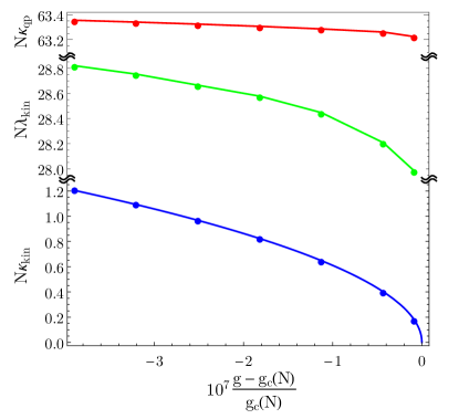
Figure 2: Numerical values of the kinetic parameters $\kappa_{\rm kin}$, $\lambda_{\rm kin}$ together with the inverse quasiparticle lifetime $\kappa_{\rm qp}$. $\kappa_{\text{kin}}$ is fitted with the scaling law (9) (blue line). The parameters used are $\kappa=2$, $\omega_{0}=2$, $\omega_{z}=2.1$ and $N=1000$, resulting in $g_{c}\approx 1.4491$. In the Appendix C we present results for $\kappa=0.2,1.0$.

III.2 Criticality and scaling laws

At any given $1\ll N<\infty$, sufficiently far away from the critical point: $(g_{c}(N)-g)/g_{c}(N)\gtrsim N^{-1/2}$, we are in a weak-coupling regime (region I in Fig. 1) where the quasiparticle interactions from $\hat{H}^{\prime}$ are always perturbative so that, to order $1/N$, the GFs follow the integrable dynamics illustrated above: $\kappa_{\rm kin}\simeq\kappa_{\rm qp}\gg\lambda_{\rm kin}$. Instead, for a quench to strong coupling $(g_{c}(N)-g)/g_{c}(N)\lesssim N^{-1/2}$ (region II in Fig. 1) the interactions appreciably renormalize the dampings such that $\kappa_{\rm kin}<\kappa_{\rm qp}$. Within this region, even closer to the critical point: $(g_{c}(N)-g)/g_{c}(N)\lesssim N^{-3/2}$, we find $\kappa_{\rm qp}\sim N^{-1/2}$ such that $\lambda_{\rm kin}$ cannot be neglected any more (see also Fig. 2). In general, the latter depends only weakly on the coupling $g$ and is also of order $N^{-1/2}$ . The role of $\lambda_{\rm kin}$ is to introduce algebraic relaxation characteristic of non-integrable dynamics. In our model without conserved quantities Torre et al. (2013) algebraic dynamics emerges due to criticality, but is in general not necessarily a signature of the latter, for instance in systems with conservation laws Hohenberg and Halperin (1977). At a given $N$-independent coupling $g$, the integrable limit of the late time dynamics is reached for $N\to\infty$ since we enter the weak coupling regime as soon as $(g_{c}(N)-g)/g_{c}(N)\gtrsim N^{-1/2}$. If instead we pin the system to criticality $(g_{c}(N)-g)/g_{c}(N)\lesssim N^{-3/2}$, the integrable limit is never approached since according to (9) $\kappa_{\rm qp}\simeq\kappa_{\rm kin}\sim N^{-1/2}\to 0$ and $\lambda_{\rm kin}\sim N^{-1/2}\to 0$, so that the non-integrable character is always important. This is related to the fact that at criticality the limits $N\to\infty$ and $\tau\to\infty$ do not commute. As a side remark, the fact that quasiparticle collisions breaking integrability become important at criticality can be seen also by analyzing the steady state. In particular, as shown in the Appendix D, integrability breaking effectively creates a bath for the spin (atomic) degree of freedom.

III.3 Algebraic vs. Exponential dynamics

An example depicting the generic behavior of the absolute-time evolution is sketched in Fig. 3 using the occupation of the quasiparticle mode $n(\tau)=iG^{K}(0,\tau)/2-1/2$ as observable. After the quench the system has to become sufficiently populated and correlated for interactions to become important. This requires a time $\tau_{\rm alg}\sim 1/\kappa_{\rm qp}$, after which the initial exponential integrable dynamics goes over into a non-integrable $1/\tau$ behavior. Deep inside the strong coupling regime: $|g_{c}(N)-g|/g_{c}(N)\lesssim N^{-3/2}$, a second crossover takes place on a scale $\tau_{\rm exp}\sim 1/\kappa_{\rm kin}$, where for $g<g_{c}(N)$ the algebraic relaxation goes back to exponential, as predicted by Eqs. (III). Using the result (9) we get the following scaling

$$\tau_{\text{exp}}\sim 1/\kappa_{\text{kin}}\sim N^{-1/4}(|g-g_{c}(N)|/g_{c}(N))^{-1/2}\;.$$ (10)

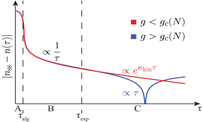
Figure 3: Sketch of a log-plot of the time evolution of the particle number near $g_{c}(N)$, separated into three regions. Starting from the vacuum, the system is for short time-scales described by the evolution according to the bare Green’s function (region A), which will then cross over into an algebraic decay (region B), that continues to infinite times for $g=g_{c}(N)$. For $g<g_{c}(N)$ the final relaxation is exponential, as depicted in region C, whereas for $g>g_{c}(N)$ the population instead evolves linearly through that of the unstable steady state.

The transcritical $g>g_{c}(N)$ time-evolution is also shown in Fig. 3. For times later than $\tau_{\text{alg}}$ the system first approaches the steady state $G_{\rm ss}^{K,R}(t_{\text{rel}})$ of Eq. (III) algebraically: $1/\tau$. However, beyond the time-scale $\tau_{\text{exp}}$ the system then evolves linearly past this unstable state with a characteristic rate given by $\partial_{\tau}\delta O\simeq\kappa^{2}_{\text{kin}}O_{\text{ss}}/\left(4\lambda_{\text{kin}}G^{K}_{\text{ss}}(0)\right)$ for any observable $O$. After the linear regime, the evolution accelerates again, becomes algebraic and would eventually converge toward the symmetry-broken steady state. The description of such a state however requires the expansion around a symmetry-broken saddle point, including (self-consistent) finite field expectation values $\langle\hat{a}\rangle$ and $\langle\hat{b}\rangle$, which is described by a more general version of Hamiltonian (3). The new steady state is therefore currently inaccessible to the presented dynamics. The sudden switch in the dynamical behavior at $g=g_{c}(N)$ characterizing the phase transition is triggered by quasiparticle collisions in presence of both Markovian losses and effective driving. In particular, since the system has weakly damped quasiparticles at $\omega_{\rm qp}=0$ (which is possible due to Markovian losses), collisions take place almost on-shell and therefore efficiently increase the mode occupation. The drive (breaking number conservation) provides the source of quasiparticles allowing the latter process to induce an instability.

III.4 Absence of ageing

For a quench exactly to the critical point $g=g_{c}(N)$, the power-law $1/\tau$ dynamics extends down to the steady state. Due to the breaking of time-translation invariance and the presence of critical algebraic relaxation even down to $\tau=\infty$ one might expect ageing to characterize the late time behavior of two-times functions Calabrese and Gambassi (2005). Such behavior has been predicted to appear after quenches to critical points both in closed Foini et al. (2011); Sciolla and Biroli (2013); Chiocchetta et al. (2015) and open Gagel et al. (2014) quantum sytems. In order to explore this possiblity we employ the fluctuation-dissipation ratio Calabrese and Gambassi (2005) $\chi_{\mathcal{O}}(t_{1},t_{2})=(G^{R}_{\mathcal{O}}(t_{1},t_{2})-G^{A}_{\mathcal{O}}(t_{1},t_{2}))/\partial_{t_{1}}G^{K}_{\mathcal{O}}(t_{1},t_{2})$ with $t_{1}<t_{2}$, which allows to address possible violations of detailed balance and define effective temperatures for non-equilibrium systems, where the fluctuation-dissipation theorem cannot be relied on. In $\chi_{\mathcal{O}}(t_{1},t_{2})$ the index $\mathcal{O}$ means that the quotient is to be taken between expectation values corresponding to the most highly occupied eigenvector of some operator $\mathcal{O}$. The limit $\lim_{t_{1}\to\infty}\lim_{t_{2}\to\infty}\chi_{\mathcal{O}}(t_{1},t_{2})\equiv 1/T_{\rm eff}$ defines an effective temperature. In systems exhibiting ageing after a quench to the critical point the equilibration time diverges. As a consequence, the effective temperature defined through the above limit will not be equal to the value of the effective temperature obtained directly from the steady state, even if the system is in contact with a thermal reservoir. Using our late-time GFs (III) it is easy to see that the fluctuation-dissipation ratio is independent of the relative time:

$$\chi(t_{\text{rel}},\tau)=\frac{1}{T_{\text{eff}}}\frac{1}{1+\frac{1}{\lambda_{\text{kin}}\kappa_{\text{qp}}\tau^{2}}}.$$ (11)

Therefore, for absolute times larger than the equilibration scale

$$\tau_{\text{eq}}=1/\sqrt{\lambda_{\text{kin}}\kappa_{\text{qp}}}$$ (12)

it relaxes to the inverse effective temperature $T_{\text{eff}}$. Since at $g_{c}(N)$ the quasiparticle lifetime remains finite $1/\kappa_{\rm qp}<\infty$, the equilibration scale $\tau_{\rm eq}$ is also finite and thus no ageing takes place. $1/\kappa_{\rm qp}<\infty$ also implies that the initial-slip exponent $\theta$ describing the $(t_{2}/t_{1})^{\theta}$ scaling of two-times functions Calabrese and Gambassi (2005) is irrelevant, since the dynamics is exponential in the relative-time direction (see Eq. (III)). However, due to the driven-dissipative nature of our system, the steady state is not in global equilibrium, implying that the effective temperature obtained from (11) depends in general on the particular degree of freedom considered, consistent with what was found in Torre et al. (2013) by extracting $T_{\text{eff}}$ directly from the steady state (see also Appendix D).

IV Predicitons for the experiment

The dynamical phase transition of the open Dicke model has been investigated in recent quench experiments performed with a Bose-Einstein condensate (BEC) in an optical cavity Klinder et al. (2015). We expect our predictions to be observable in response and correlation functions of the cavity output, once the wait-time $\tau_{\rm w}$ after the quench satisfies $\tau_{\rm w}\gtrsim\tau_{\rm alg}\sim 1/\kappa_{\rm qp}\sim N^{1/2}$ (see Section III). Generically, the smallest value of $\tau_{\rm alg}$ is reached when $\omega_{z}$ (corresponding to the recoil frequency $\omega_{\rm rec}\sim\text{KHz}$ in the BEC experiments) is of the same order of $\kappa$. This can be seen by comparing the value of $\kappa_{\rm qp}$ for different values of $\kappa=2,1,0.2$ shown in Fig. 2 and Fig. 5, at a given $\omega_{z}=2.1$. The largest $\kappa_{\rm qp}$ is reached indeed for $\kappa\simeq\omega_{z}$, while for even larger $\kappa$ (not shown) the quasiparticle damping decreases. For instance, in the experimental setup of Klinder et al. (2015) the cavity is very good: $\kappa\simeq\omega_{\rm rec}$, so that $\kappa_{\rm qp}\sim\kappa N^{-1/2}$ that is $\tau_{\rm w}\gtrsim\text{ms}\times(10^{5})^{1/2}\sim 300{\rm ms}$. While this is below typical BEC-lifetimes, it is currently not achieved in the experiments Klinder et al. (2015), but in principle possible in the new-generation setups.

While the measurement of response functions require cavity probe-transmission experiments Dimer et al. (2007); Torre et al. (2013), the behavior of the correlation function in Fig. 3 will be directly observable from the cavity output intensity.

V Conclusions

We have shown that the dynamics following a quench close to a critical point in an open quantum many-body system can depend crucially on the competition between external and intrinsic relaxation processes, the former due to drive and dissipation, the latter due to integrability breaking through quasiparticle interactions. In particular, we demonstrated a novel scenario involving a dynamical phase transition where critical algebraic relaxation is not accompanied by ageing, due to the finite lifetime of quasiparticles. The simplicity and paradigmatic character of the model considered allowed for a detailed understanding of the phenomena and should imply a broader relevance of our results.

Appendix A Keldysh formulation of the self-consistent Hartree-Fock theory

The open Dicke model introduced in the main text has already been formulated within the Keldysh functional-integral framework Torre et al. (2013), thus we only briefly discuss the main features here. We then describe the self-consistent Hartree-Fock (SCHF) theory we employ.

Starting from the master equation, the functional-integral formulation of the action is achieved by replacing the operators acting left(right) of the density matrix with complex fields with a subscript “$+$”(“$-$”). Calculating expectation values by a time-evolution along the Keldysh contour, the “$+$”operators act while the system evolves forward in time, while the “$-$”operators act on the backward branch. It is easier to obtain physical insight by rotating to “classical”  $a_{cl}=\frac{1}{\sqrt{2}}\left(a_{+}+a_{-}\right)$ and “quantum” fields $a_{q}=\frac{1}{\sqrt{2}}\left(a_{+}-a_{-}\right)$, that deserve their name because only “classical”  fields can propagate on-shell or have a finite expectation value Kamenev (2011), whereas “quantum”  fields encode the (potentially correlated) statistical noise in an equivalent Langevin formulation. Due to the loss of particle number conservation it is convenient to symmetrize the action through the identification of terms between advanced and retarded contributions. The symmetrized action of $\hat{H}_{0}$ in the absence of coherent fields then reads Torre et al. (2013)

$$S_{0}=\int\frac{d\omega}{2\pi}V^{\dagger}(\omega)\begin{pmatrix}0&&\left[G^{A}_{0}\right]^{-1}(\omega)\\ \left[G^{R}_{0}\right]^{-1}(\omega)&&D^{K}(\omega)\\ \end{pmatrix}V(\omega)$$ (13)

because retarded and advanced Green’s functions interchange under $\omega\rightarrow-\omega$. The bare inverse GFs $\left[G^{R}_{0}\right]^{-1}(\omega)$ and $D_{0}^{K}$ are given by

$$\left[G^{R}_{0}\right]^{-1}(\omega)=$$

$$\begin{pmatrix}\omega-\omega_{0}+i\kappa&&0&&-g&&-g\\ 0&&-\omega-\omega_{0}-i\kappa&&-g&&-g\\ -g&&-g&&\omega-\omega_{z}&&0\\ -g&&-g&&0&&-\omega-\omega_{z}\\ \end{pmatrix}$$

 and

$$D_{0}^{K}=$$

$$\begin{pmatrix}2i\kappa&&0&&0&&0\\ 0&&2i\kappa&&0&&0\\ 0&&0&&0&&0\\ 0&&0&&0&&0\\ \end{pmatrix}.$$ (14)

The verbose notation with the eight-component field

$$V(\omega)=\left(\begin{array}[]{c}a_{cl}(\omega)\\ a_{cl}^{*}(-\omega)\\ b_{cl}(\omega)\\ b_{cl}^{*}(-\omega)\\ a_{q}(\omega)\\ a_{q}^{*}(-\omega)\\ b_{q}(\omega)\\ b_{q}^{*}(-\omega)\end{array}\right).$$ (23)

is necessary, since each – Keldysh ($cl,q$) and Nambu ($\omega,-\omega$) structure – double the number of fields compared to the quantum mechanical representation.

For $N<\infty$, the terms of the quartic interaction Hamiltonian $\hat{H}^{\prime}$ in Eq. (3) have to be added to the action in (13). Considering the possibility of interactions on the forward and the backward branch of the Keldysh contour, the corresponding part of the action reads

$$\begin{split}S_{\text{int}}&=\frac{g}{4N}\int\frac{d\omega}{2\pi}\bigg{[}\left[\left(a_{cl}+a_{cl}^{*}\right)\circ\left(b_{q}+b_{q}^{*}\right)+\left(a_{q}+a_{q}^{*}\right)\circ\left(b_{cl}+b_{cl}^{*}\right)\right]\circ\left[b_{cl}^{*}b_{cl}+b_{q}^{*}b_{q}\right]\\ &+\left[\left(a_{cl}+a_{cl}^{*}\right)\circ\left(b_{cl}+b_{cl}^{*}\right)+\left(a_{q}+a_{q}^{*}\right)\circ\left(b_{q}+b_{q}^{*}\right)\right]\circ\left[b_{cl}^{*}b_{q}+b_{q}^{*}b_{cl}\right]\bigg{]}(\omega),\end{split}$$ (24)

where “$\circ$” denotes the convolution in $\omega$ (normalized by $1/(2\pi)$).

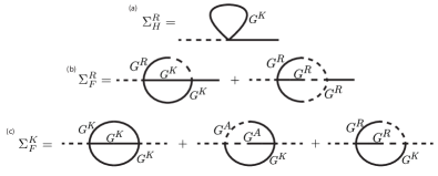
Figure 4: Self-energy diagrams used in the SCHF calculations. The Hartree contribution (a) is only a real shift of the retarded component. The Fock contribution (b) and (c) is instead complex and frequency-dependent. Here the solid(dashed) line correspond to a “classical”(“quantum”) field attached to the vertex.

The results presented in the main text are obtained within a self-consistent Hartree-Fock (SCHF) approximation, corresponding to the selection of diagrams for the self-energies shown in Fig. 4. The self-consistent Hartree (SCH) approach has already been treated by Dalla Torre et al in Torre et al. (2013) for the steady state. As we illustrate next, the inclusion of the Fock processes we perform here is required to describe the effect of non-number-conserving quasiparticle collisions breaking the integrability. These collisions are essential ingredients in the steady state and late-time relaxation dynamics of the system close to the superradiant transition. Self-consistency is achieved by calculating the self-energies $\Sigma^{(K,R)}$ as functionals of the dressed, rather than the bare Green’s functions: $\Sigma^{(K,R)}=\Sigma^{(K,R)}\!\!\left[G^{R},G^{K}\right]$. In order to highlight the novelties introduced by our SCHF approach, we now briefly discuss the main features of the SCH theory.

Within the Hartree approximation only one skeleton diagram contributes to the self-energies. Furthermore, because $G^{R}(0)+G^{A}(0)=0$ only the retarded/advanced self-energy, given by the first diagram in Fig. 4, is non-zero. The resulting frequency-independent self-consistence condition can be solved (mostly) analytically and predicts that both $\kappa_{\text{qp}}$ and the number of excitations in the steady state remain finite for all values of the coupling constant. Furthermore, it can be shown that the steady state is attractive under time-evolution for any coupling strength, implying that no dynamical phase transition occurs on the self-consistent one-loop level.

The theory becomes much more involved within the SCHF approach we employ here. First of all, the Fock self-energy of Fig. 4 is frequency-dependent as opposed to its Hartree counterpart. This enriches the problem by allowing for the inclusion of memory effects, which however play no significant role near the superradiant transition. Additionally, the Keldysh component of the Fock self-energy is nonzero and the retarded component has an imaginary part. This implies that the inclusion of the Fock processes in our theory allows us to describe relaxation through redistribution of energy via collisions between quasiparticles.
Within this approximation there are two different subclasses of diagrams: those involving only one ”quantum” field and those with three ”quantum” fields. A bare scaling analysis of the model (13),(24) indicates that the latter are of higher order in $1/N$ compared to the more classical first subset of diagrams Torre et al. (2013). Yet, in order to improve our quantitative results for intermediate values of $N$ as well as for the phase transition, we keep those diagrams. Independent of this, the self-consistent resummation of two-loop diagrams cannot be performed analytically forcing us to heavily rely on numerical methods for the calculation of quantitative results. However, all the analytical expressions in the main text are completely independent of the numerics, that can therefore – as done in figure 2 of the main text– be used for independent confirmation.

Appendix B Time-integration of the coupled Dyson equations

Within the SCHF approximation, we perform a time integration of the coupled, nonlinear Dyson equations (5) and (6) for the Keldysh and retarded GFs. We adopt an iteration procedure valid in the vicinity of the steady state:

$$G^{R}(\tau+\delta\tau)=(1-c)G^{R}(\tau)+c\left(\left[G^{R}_{0}\right]^{-1}-\Sigma^{R}\left(G^{R}(\tau)\right)\right)^{-1}$$ (25)

where $c$ is the numerical update in our iteration, $\tau$ is the absolute time and we suppressed the dependence of the GF on the relative time $t_{\rm rel}$. Here the subscript ss stands for steady state. Since including the dynamics for the Keldysh component contributes only further additive terms with the same global prefactors, we simplify the expressions here to depend solely on the retarded Green’s function. We see how the approximate time-iteration (25) neglects memory effects involving time-integrals over the past, so that solutions of the form Eq. (7) of the main text can be found, where the $t_{\rm rel}$-functional form depends only parametrically on $\tau$ through $\kappa_{\rm qp}(\tau)$. The $\tau$-dependence of the latter is of order $1/N$ and thus negligible. The approximation involved in (25) relies on a separation of timescales between the relative and absolute time-evolution and is equivalent to taking the leading order in the Wigner expansion of the convolutions between two-times functions Note (1):

$$A\circ B=\int dt_{3}A(t_{1},t_{3})B(t_{3},t_{2})$$

$$\overset{WT}{\Leftrightarrow}A(\tau,\omega)e^{\frac{i}{2}\left(\overset{\leftarrow}{\partial_{\omega}}\overset{\rightarrow}{\partial_{\tau}}-\overset{\leftarrow}{\partial_{\tau}}\overset{\rightarrow}{\partial_{\omega}}\right)}B(\tau,\omega)\simeq A(\tau,\omega)B(\tau,\omega),$$ (26)

where we defined $f(t_{1},t_{2})\overset{WT}{\Leftrightarrow}f(\tau,\omega)=\int dt_{\rm rel}e^{-i\omega t_{\rm rel}}f(\tau-t_{\rm rel}/2,\tau+t_{\rm rel}/2)$. The required separation of timescales is achieved in our system in the vicinity of the steady state and for a quench of $g$ close enough to $g_{c}(N)$. As Fig.1 shows, in this regime $\kappa_{\rm kin}$, setting the absolute timescale (see Eq.(7)), is much smaller than $\kappa_{\rm qp}$. The latter, setting the relative timescale, remains indeed finite at our dynamical phase transition. For the same reasons, our numerical time-evolution is not applicable well inside the weak-coupling regime (region I of Fig.1 in the main text), since there $\kappa_{\rm kin}\simeq\kappa_{\rm qp}$.

Appendix C Role of the photon loss rate $\kappa$

In this section we complement the results presented in the main text by computing the dynamical parameters $\kappa_{\rm qp}$, $\kappa_{\rm kin}$, $\lambda_{\rm kin}$ for smaller values of the photon loss rate $\kappa$. The goal is to illustrate the qualitative behavior of the system in the isolated limit $\kappa\to 0$. In Fig. 5 we show the results for $\kappa=1$ and $\kappa=0.2$, to be compared with Fig. 2 of the main text, computed for $\kappa=2$. Two main observations emerge: i) since all the dynamical parameters ($\kappa_{\rm qp}$, $\kappa_{\rm kin}$ , $\lambda_{\rm kin}$) decrease for decreasing $\kappa$, the global timescale becomes slower; ii) since $\kappa_{\rm qp}$ and $\kappa_{\rm kin}$ become closer to one another, it becomes more difficult (i.e. one has to tune the system even closer to $g_{c}(N)$) to reach the dynamical critical regime where $\kappa_{\rm in}\ll\kappa_{\rm qp}$. Ultimately, in the $\kappa=0$ limit, we expect $\kappa_{\rm kin}$ to become coupled to $\kappa_{\rm qp}$, in the sense that the former cannot be made arbitrarily small compared to the latter, at any given $N$. The numerical computation leading to a set of results as the one in Fig. 5 is very demanding and becomes more and more so a $\kappa\to 0$, since the global timescale becomes slower and $\kappa_{\rm kin}\to\kappa_{\rm qp}$ (see previous section). Our approach is not applicable in the case $\kappa=0$.

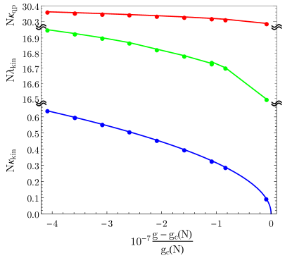
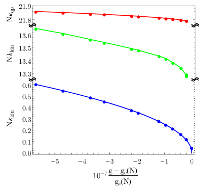
Figure 5: Numerical values of the kinetic parameters $\kappa_{\text{kin}}$, $\lambda_{\text{kin}}$ as well as the inverse quasiparticle lifetime $\kappa_{\text{qp}}$. The parameters used are the same as in the main text, apart from $\kappa=1$ (upper panel) and $\kappa=0.2$ (lower panel), which result in $g_{c}\approx 1.1420$ and $g_{c}\approx 1.0298$ respectively.

Appendix D The steady-state distribution function

In this section we consider the steady-state of the coupled-Dyson equations (5) and (6) of the main text. We will show how the integrability-breaking through quasiparticle interactions leads to equilibration. This intrinsic equilibration adds to the one induced by the coupling to the external reservoir.

To this purpose, we consider the steady-state distribution function $F(\omega)$ defined through

$$G^{K}(\omega)=G^{R}(\omega)\cdot F(\omega)-F(\omega)\cdot G^{A}(\omega).$$ (27)

The function $F(\omega)$ determines the link between response and correlation functions and is therefore deeply connected with the fluctuation-dissipation relations in the steady state Kamenev (2011). $F(\omega)$ describes the boundary conditions emergent in the steady state for each degree of freedom of our system. For instance, for a single bosonic degree of freedom in thermal equilibrium with a reservoir at temperature $T$, the distribution function $F(\omega)$ is simply $\coth(\omega/2T)$ Kamenev (2011), while for a Markov reservoir corresponding to the Lindblad operator (2) of the main text we have $F(\omega)=1$, corresponding to a pure state Torre et al. (2013). One can thus expect $F(\omega)$ to be sensitive to the different drive and relaxation mechanisms, both external and intrinsic to the system.

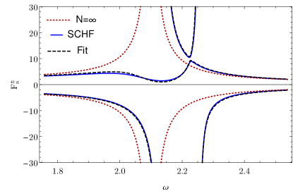
Figure 6: Behavior of the two eigenvalues of the photonic distribution function. The red-dotted line corresponds to the integrable theory: $N=\infty$. The blue solid line is the result obtained from full SCHF theory, where qualitatively new features appear. These can be well described by an effective linearised theory Eq. (D) (black-dashed line) that shifts the atomic resonance in the complex plane and therefore contains only a single (complex) fit parameter $\kappa_{b}$. The parameters used are the same as in the main text, resulting in $\kappa_{b}\approx 0.0335+0.0009i$.

In order to analyze the distribution function for the photonic and atomic degrees of freedom separately, we have first projected the full 4 by 4 Green’s functions onto the respective 2 by 2 sectors. Within each sector we then solved (27) for $F_{a}(\omega)$ and $F_{b}(\omega)$, respectively, where the subscript $a$ refers to the photonic and $b$ to the atomic sector Note (1). In Fig. 6, we plot the eigenvalues $F^{\pm}_{a}(\omega)$ of $F_{a}(\omega)$, which due to the hermitian structure of $F(\omega)$ are purely real.

In our open Dicke model and in the integrable limit $N=\infty$, external driving is effectively present due to the bilinear coupling between photonic and atomic degrees of freedom which does not conserve the excitation number, while relaxation is induced externally by photon losses. As discussed in Torre et al. (2013), the corresponding distribution function for the photonic degree of freedom shows singularities at zero frequency and at the bare atomic resonance frequencies $\pm\omega_{z}$. These singularities appear on top of the frequency-independent Markov background and result from the effective drive via the atoms. These singularities are of thermal nature, behaving like $T_{\rm eff}/\omega$, with the effective temperature emerging due to the combination of the Markov reservoir and the driving. This temperature is different for the photonic and atomic degrees of freedom, indicating the violation of detailed balance arising from the fact that the whole system is driven but dissipates only through the photons (see also section III.4).

Within our SCHF approach, we are able to include the equilibration mechanism intrinsic to the system, which is governed by the integrability-breaking terms. In particular, as already discussed, the Fock processes allow to include the intrinsic equilibration induced by quasiparticle collisions. In the strong coupling regime: $(g_{c}(N)-g)/g_{c}(N)\lesssim N^{-1/2}$, this introduces large qualitative and quantitative changes in $F(\omega)$, as illustrated in Fig. 6 for the photonic degree of freedom. Here we compare the prediction of the integrable theory: $N=\infty$ with our SCHF results. Apart from a shift of the singularities from their bare value $\omega_{z}$, the important qualitative change introduced by collisions is the splitting of these singularities via an avoided crossing. This splitting of the singularities at the (shifted) atomic resonances can be reproduced by adding to the integrable theory a second Markov reservoir, this time for the atomic degree of freedom. This corresponds to the steady-state of the following master equation

$$\partial_{t}\rho =-i\left[\hat{H}_{0},\rho\right]$$

$$+\kappa\left(2\hat{a}\rho\hat{a}^{\dagger}-\left\{\hat{a}^{\dagger}\hat{a},\rho\right\}\right)+\kappa_{b}\left(2\hat{b}\rho\hat{b}^{\dagger}-\left\{\hat{b}^{\dagger}\hat{b},\rho\right\}\right).$$ (28)

where $\hat{H}_{0}$ indicates the integrable Hamiltonian of Eq.(3). By choosing the effective atomic dissipation $\kappa_{b}$ appropriately (including the shift of the resonance frequency), we can simulate the extent to which the quasiparticle collisions result in enhanced decay of atomic excitations into multiple photons. This demonstrates how the integrability-breaking leads to enhanced equilibration by creating effectively a further bath for the the system.

While $F(\omega)$ contains a lot of information encoded in its functional form, its measurement requires knowledge of both the spectral response and the correlation functions. The former gives direct access to the retarded (and by complex conjugation the advanced) Green’s function while the latter directly corresponds to the Keldysh Green’s function. Eq. (27) would then allow to compute the distribution function.

References

- Polkovnikov et al. (2011) A. Polkovnikov, K. Sengupta, A. Silva, and M. Vengalattore, Rev. Mod. Phys., 83, 863 (2011).
- Eisert et al. (2015) J. Eisert, M. Friesdorf, and C. Gogolin, Nat Phys, 11, 124 (2015).
- Diehl et al. (2008) S. Diehl, A. Micheli, A. Kantian, B. Kraus, H. Büchler, and P. Zoller, Nature Physics, 4, 878 (2008).
- Hohenberg and Halperin (1977) P. C. Hohenberg and B. I. Halperin, Reviews of Modern Physics, 49, 435 (1977).
- Calabrese and Gambassi (2005) P. Calabrese and A. Gambassi, Journal of Physics A: Mathematical and General, 38, R133 (2005).
- Mitra et al. (2006) A. Mitra, S. Takei, Y. B. Kim, and A. J. Millis, Phys. Rev. Lett., 97, 236808 (2006).
- Patanè et al. (2008) D. Patanè, A. Silva, L. Amico, R. Fazio, and G. E. Santoro, Phys. Rev. Lett., 101, 175701 (2008).
- Diehl et al. (2010) S. Diehl, A. Tomadin, A. Micheli, R. Fazio, and P. Zoller, Phys. Rev. Lett., 105, 015702 (2010).
- Dalla Torre et al. (2010) E. G. Dalla Torre, E. Demler, T. Giamarchi, and E. Altman, Nat Phys, 6, 806 (2010).
- Klaers et al. (2010) J. Klaers, J. Schmitt, F. Vewinger, and M. Weitz, Nature, 468, 545 (2010).
- Kessler et al. (2012) E. M. Kessler, G. Giedke, A. Imamoglu, S. F. Yelin, M. D. Lukin, and J. I. Cirac, Phys. Rev. A, 86, 012116 (2012).
- Kirton and Keeling (2013) P. Kirton and J. Keeling, Physical review letters, 111, 100404 (2013).
- Sieberer et al. (2013) L. M. Sieberer, S. D. Huber, E. Altman, and S. Diehl, Phys. Rev. Lett., 110, 195301 (2013).
- Täuber and Diehl (2014) U. C. Täuber and S. Diehl, Phys. Rev. X, 4, 021010 (2014).
- Bonnes et al. (2014) L. Bonnes, D. Charrier, and A. M. Läuchli, Phys. Rev. A, 90, 033612 (2014).
- Marcuzzi et al. (2014) M. Marcuzzi, E. Levi, S. Diehl, J. P. Garrahan, and I. Lesanovsky, Phys. Rev. Lett., 113, 210401 (2014).
- Hoening et al. (2014) M. Hoening, W. Abdussalam, M. Fleischhauer, and T. Pohl, Phys. Rev. A, 90, 021603 (2014).
- Medvedyeva et al. (2015) M. V. Medvedyeva, M. T. Čubrović, and S. Kehrein, Phys. Rev. B, 91, 205416 (2015).
- Labouvie et al. (2015) R. Labouvie, B. Santra, S. Heun, and H. Ott, ArXiv e-prints (2015), arXiv:1507.05007 [quant-ph] .
- Maghrebi and Gorshkov (2015) M. F. Maghrebi and A. V. Gorshkov, arXiv preprint arXiv:1507.01939 (2015).
- Marino and Diehl (2016) J. Marino and S. Diehl, Phys. Rev. Lett., 116, 070407 (2016).
- Marino and Silva (2012) J. Marino and A. Silva, Phys. Rev. B, 86, 060408 (2012).
- Sedlmayr et al. (2013) N. Sedlmayr, J. Ren, F. Gebhard, and J. Sirker, Phys. Rev. Lett., 110, 100406 (2013).
- Cai and Barthel (2013) Z. Cai and T. Barthel, Phys. Rev. Lett., 111, 150403 (2013).
- Horstmann et al. (2013) B. Horstmann, J. I. Cirac, and G. Giedke, Phys. Rev. A, 87, 012108 (2013).
- Foss-Feig et al. (2013) M. Foss-Feig, K. R. A. Hazzard, J. J. Bollinger, and A. M. Rey, Phys. Rev. A, 87, 042101 (2013).
- Gagel et al. (2014) P. Gagel, P. P. Orth, and J. Schmalian, Phys. Rev. Lett., 113, 220401 (2014).
- Piazza and Strack (2014) F. Piazza and P. Strack, Phys. Rev. A, 90, 043823 (2014).
- Schütz and Morigi (2014) S. Schütz and G. Morigi, Phys. Rev. Lett., 113, 203002 (2014).
- Schütz et al. (2015) S. Schütz, S. B. Jäger, and G. Morigi, Phys. Rev. A, 92, 063808 (2015).
- Sciolla et al. (2015) B. Sciolla, D. Poletti, and C. Kollath, Phys. Rev. Lett., 114, 170401 (2015).
- Buchhold and Diehl (2015) M. Buchhold and S. Diehl, Phys. Rev. A, 92, 013603 (2015).
- Blatt and Roos (2012) R. Blatt and C. Roos, Nature Physics, 8, 277 (2012).
- Britton et al. (2012) J. W. Britton, B. C. Sawyer, A. C. Keith, C.-C. J. Wang, J. K. Freericks, H. Uys, M. J. Biercuk, and J. J. Bollinger, Nature, 484, 489 (2012).
- Carusotto and Ciuti (2013) I. Carusotto and C. Ciuti, Rev. Mod. Phys., 85, 299 (2013).
- Hartmann et al. (2008) M. J. Hartmann, F. Brandao, and M. B. Plenio, Rev, 2, 527 (2008).
- Houck et al. (2012) A. A. Houck, H. E. Türeci, and J. Koch, Nature Physics, 8, 292 (2012).
- Schmidt and Koch (2013) S. Schmidt and J. Koch, Annalen der Physik, 525, 395 (2013).
- Ludwig and Marquardt (2013) M. Ludwig and F. Marquardt, Physical review letters, 111, 073603 (2013).
- Vetsch et al. (2010) E. Vetsch, D. Reitz, G. Sagué, R. Schmidt, S. T. Dawkins, and A. Rauschenbeutel, Phys. Rev. Lett., 104, 203603 (2010).
- Ritsch et al. (2013) H. Ritsch, P. Domokos, F. Brennecke, and T. Esslinger, Rev. Mod. Phys., 85, 553 (2013).
- Goban et al. (2014) A. Goban, C. L. Hung, S. P. Yu, J. D. Hood, J. A. Muniz, J. H. Lee, M. J. Martin, A. C. McClung, K. S. Choi, D. E. Chang, O. Painter, and H. J. Kimble, Nat Commun, 5 (2014).
- Douglas et al. (2015) J. S. Douglas, H. Habibian, C. L. Hung, A. V. Gorshkov, H. J. Kimble, and D. E. Chang, Nat Photon, 9, 326 (2015).
- Dimer et al. (2007) F. Dimer, B. Estienne, A. S. Parkins, and H. J. Carmichael, Phys. Rev. A, 75, 013804 (2007).
- Keeling et al. (2010) J. Keeling, M. J. Bhaseen, and B. D. Simons, Phys. Rev. Lett., 105, 043001 (2010).
- Bhaseen et al. (2012) M. J. Bhaseen, J. Mayoh, B. D. Simons, and J. Keeling, Phys. Rev. A, 85, 013817 (2012).
- Öztop et al. (2012) B. Öztop, M. Bordyuh, O. E. Müstecaplioglu, and H. E. Türeci, New Journal of Physics, 14, 085011 (2012).
- Kónya et al. (2012) G. Kónya, D. Nagy, G. Szirmai, and P. Domokos, Phys. Rev. A, 86, 013641 (2012).
- Nagy et al. (2011) D. Nagy, G. Szirmai, and P. Domokos, Phys. Rev. A, 84, 043637 (2011).
- Torre et al. (2013) E. G. D. Torre, S. Diehl, M. D. Lukin, S. Sachdev, and P. Strack, Phys. Rev. A, 87, 023831 (2013).
- Tomka et al. (2013) M. Tomka, D. Baeriswyl, and V. Gritsev, Phys. Rev. A, 88, 053801 (2013).
- Genway et al. (2014) S. Genway, W. Li, C. Ates, B. P. Lanyon, and I. Lesanovsky, Phys. Rev. Lett., 112, 023603 (2014).
- Nagy and Domokos (2015) D. Nagy and P. Domokos, Phys. Rev. Lett., 115, 043601 (2015).
- Acevedo et al. (2015) O. L. Acevedo, L. Quiroga, F. J. Rodríguez, and N. F. Johnson, New Journal of Physics, 17, 093005 (2015).
- Dicke (1954) R. H. Dicke, Phys. Rev., 93, 99 (1954).
- Hepp and Lieb (1973) K. Hepp and E. H. Lieb, Annals of Physics, 76, 360 (1973), ISSN 0003-4916.
- Wang and Hioe (1973) Y. K. Wang and F. T. Hioe, Phys. Rev. A, 7, 831 (1973).
- Lambert et al. (2004) N. Lambert, C. Emary, and T. Brandes, Phys. Rev. Lett., 92, 073602 (2004).
- Vidal and Dusuel (2006) J. Vidal and S. Dusuel, EPL (Europhysics Letters), 74, 817 (2006).
- Liu et al. (2009) T. Liu, Y.-Y. Zhang, Q.-H. Chen, and K.-L. Wang, Phys. Rev. A, 80, 023810 (2009).
- Larson and Lewenstein (2009) J. Larson and M. Lewenstein, New Journal of Physics, 11, 063027 (2009).
- Nagy et al. (2010) D. Nagy, G. Kónya, G. Szirmai, and P. Domokos, Phys. Rev. Lett., 104, 130401 (2010).
- Mumford et al. (2014) J. Mumford, J. Larson, and D. H. J. O’Dell, Phys. Rev. A, 89, 023620 (2014).
- Baumann et al. (2010) K. Baumann, C. Guerlin, F. Brennecke, and T. Esslinger, Nature, 464, 1301 (2010).
- Baumann et al. (2011) K. Baumann, R. Mottl, F. Brennecke, and T. Esslinger, Phys. Rev. Lett., 107, 140402 (2011).
- Brennecke et al. (2013) F. Brennecke, R. Mottl, K. Baumann, R. Landig, T. Donner, and T. Esslinger, Proceedings of the National Academy of Sciences, 110, 11763 (2013).
- Baden et al. (2014) M. P. Baden, K. J. Arnold, A. L. Grimsmo, S. Parkins, and M. D. Barrett, Phys. Rev. Lett., 113, 020408 (2014).
- Keßler et al. (2014) H. Keßler, J. Klinder, M. Wolke, and A. Hemmerich, Phys. Rev. Lett., 113, 070404 (2014).
- Klinder et al. (2015) J. Klinder, H. Keßler, M. Wolke, L. Mathey, and A. Hemmerich, Proceedings of the National Academy of Sciences, 112, 3290 (2015).
- Fagotti and Essler (2013) M. Fagotti and F. H. L. Essler, Phys. Rev. B, 87, 245107 (2013).
- Emary and Brandes (2003) C. Emary and T. Brandes, Phys. Rev. E, 67, 066203 (2003).
- Bakemeier et al. (2013) L. Bakemeier, A. Alvermann, and H. Fehske, Phys. Rev. A, 88, 043835 (2013).
- Altland and Haake (2012) A. Altland and F. Haake, Phys. Rev. Lett., 108, 073601 (2012).
- Buchhold et al. (2013) M. Buchhold, P. Strack, S. Sachdev, and S. Diehl, Phys. Rev. A, 87, 063622 (2013).
- Kulkarni et al. (2013) M. Kulkarni, B. Öztop, and H. E. Türeci, Phys. Rev. Lett., 111, 220408 (2013).
- Kónya et al. (2014) G. Kónya, G. Szirmai, and P. Domokos, Phys. Rev. A, 90, 013623 (2014).
- Kamenev (2011) A. Kamenev, Field Theory of Non-Equilibrium Systems (Cambridge University Press, 2011) ISBN 9781139500296.
- Sieberer et al. (2015) L. Sieberer, M. Buchhold, and S. Diehl, arXiv preprint arXiv:1512.00637 (2015).
- Note (1) See Supplemental Material.
- Marcuzzi et al. (2013) M. Marcuzzi, J. Marino, A. Gambassi, and A. Silva, Phys. Rev. Lett., 111, 197203 (2013).
- Note (2) Note that the single-mode approximation, implicit in the results presented here, breaks down for small coupling constants, where and the two most relevant modes have degenerate lifetimes.
- Note (3) The scaling laws we found for , and can be also derived from the scale-invariance of the GFs, which holds in the strong-coupling region. See J. Lang and F. Piazza, in preparation (2016).
- Foini et al. (2011) L. Foini, L. F. Cugliandolo, and A. Gambassi, Phys. Rev. B, 84, 212404 (2011).
- Sciolla and Biroli (2013) B. Sciolla and G. Biroli, Phys. Rev. B, 88, 201110 (2013).
- Chiocchetta et al. (2015) A. Chiocchetta, M. Tavora, A. Gambassi, and A. Mitra, Phys. Rev. B, 91, 220302 (2015).
- Note (4) J. Lang and F. Piazza, in preparation (2016).