On the Compton scattering redistribution function in plasma

Abstract

Compton scattering is the dominant opacity source in hot neutron stars, accretion disks around black holes and hot coronae. We collected here a set of numerical expressions of the Compton scattering redistribution functions for unpolarized radiation (RF) , which are more exact than the widely used Kompaneets equation. The principal aim of this paper is presentation of the RF by Guilbert (1981) which is corrected for the computational errors in the original paper. This corrected RF was used in the series of papers on model atmosphere computations of hot neutron stars. We have also organized four existing algorithms for the RF computations into a unified form ready to use in radiative transfer and model atmosphere codes. The exact method by Nagirner and Poutanen (1993) was numerically compared to all other algorithms in a very wide spectral range from hard X-rays to radio waves. Sample computations of the Compton scattering redistribution functions in thermal plasma were done for temperatures corresponding to the atmospheres of bursting neutron stars and hot intergalactic medium. Our formulae are also useful to the study Compton scattering of unpolarised microwave background radiation in hot intra-cluster gas and the Sunyaev-Zeldovich effect. We conclude, that the formulae by Guilbert (1981) and the exact quantum mechanical formulae yield practically the same redistribution functions for gas temperatures relevant to the atmospheres of X-ray bursting neutron stars, $T\leq 10^{8}$ K.

1 Introduction

Compton scattering of unpolarized photons on free thermal electrons plays a crucial role in continuum and line spectrum formation in various astrophysical objects. The essential features of the scattering are a random change of direction of photon propagation and an exchange of energy and momentum between colliding particles. Compton scattering is a dominant source of continuum opacity in very hot DA white dwarfs and unmagnetized neutron stars and is responsible for the continuum spectrum formation in Type I X-ray bursters. In other objects Compton scattering influences the line spectrum of OB giant or main sequence stars. In the X-ray domain, Compton scattering of external irradiation creates the Compton shoulder of fluorescent iron $K_{\alpha}$ lines at 6.4 keV in the spectra of active galactic nuclei and galactic black hole binaries.

The scattering is an intrinsically strongly nonisotropic process, which also depends on the state of the incident photon polarization. However, herein, we consider the angle-averaged Compton scattering of unpolarized thermal radiation in the absence of a magnetic field. Such an averaged process can be best described by a redistribution function (RF), which gives the probability density of photon energy and the momentum change upon scattering.

Compton scattering of unpolarized radiation has been studied in a number of papers in the literature and the most pertinent to the present study being those of Buchler and Yueh (1976), Guilbert (1981), Nagirner and Poutanen (1993), Poutanen (1994), Sazonov and Sunyaev (2000) and Poutanen and Vurm (2010). Paper by Younsi and Wu (2013) defined general relativistic Compton redistribution function and its moments.

In this paper we present set of equations which define the RF derived by Guilbert (1981) which is corrected here for the computational errors in the latter paper. This corrected RF was used in the series of papers on model atmosphere computations of hot neutron stars starting from Madej (1989) and extended also to irradiated relativistic accretion disks, cf. Madej & Różańska (2000).

Herein we compared the procedure by Guilbert (1981) with the exact quantum mechanical method summarized by Suleimanov et al. (2012), Appendix A, and with two other approximate algorithms. All assume that isotropic plasma is nondegenerate with fully relativistic electron thermal velocities.

Furthermore, we collected the formulae derived in other published papers describing the redistribution of Compton scattered photons over energies and scattering angles. Our aim was to obtain expressions for Compton scattering cross sections and kernels (Pomraning 1973) that would be useful in a very wide range of temperatures and frequencies.

Section 2 thus presents a list of equations and auxiliary variables that allow for the determination of Compton scattering cross-sections in unified form following various methods. We do not aim to discuss or evaluate the corresponding physical assumptions or approximations used in the original papers. Instead, our paper is rather a description and purely numerical tests of the new code (now publicly available) for RF computations using several available algorithms.

Section 3 presents the exact Compton redistribution function derived by Nagirner and Poutanen (1993), Poutanen and Vurm (2010) and Suleimanov et al. (2012). Section 4 presents the Compton redistribution formulae by Guilbert (1981), but corrected for computational errors in the original paper. Guilbert’s and exact approaches implement Klein-Nishina scattering cross-sections from electrons at rest. For a completeness, both angle-dependent cross-sections were compared to a third, approximate formula obtained assuming that electron scattering is isotropic with classical Thomson cross-sections in the electron rest frame (Poutanen & Svensson 1996; Suleimanov et al. 2012). Fourth formula was taken from Sazonov and Sunyaev (2000), see Eqs. 7a-7d therein.

2 Compton scattering redistribution function

Here, the key variable is $R\,(\nu,\nu^{\prime},\eta)$, which denotes the probability of scattering a photon with an initial frequency $\nu$ at a unit solid angle $d\Omega$ and unit frequency range at a final frequency $\nu^{\prime}$ (in Hz), counted per unit distance along the ray path. Variable $\eta=\cos\theta$ is the cosine of a scattering angle $\theta$. Variable $R$ is equal to the differential scattering coefficient $\sigma(\nu\rightarrow\nu{{}^{\prime}},\vec{n}\cdot\vec{n}{{}^{\prime}})$ defined by Pomraning (1973), see Eq. 1-31 therein.

Function $R\,(\nu,\nu^{\prime},\eta)$ was also integrated over the solid angle $d\Omega$. The angle-integrated redistribution function $R(\nu,\nu^{\prime})$ (the Compton scattering kernel) is then given in Hz^-1.

The scattering electrons in the plasma of temperature $T$ have a thermal relativistic Maxwellian velocity distribution given by

$$f_{e}\,(p)={1\over{4\pi\,\Theta\,K_{2}(1/\Theta)}}\,\exp(-\gamma/\Theta)\,,\hskip 28.45274pt{\rm where}\hskip 8.53581pt\Theta=kT/m_{e}c^{2}\,.$$ (1)

and $\gamma$ denotes the electron Lorentz factor.

The following sections 3-5 present four different algorithms for the computation of the Compton scattering redistribution function in a unified form, suitable for the radiative transfer calculations. Algorithms were either corrected for fatal algebraic errors (Guilbert 1981) or reexpressed to a more optimal form than that given in Suleimanov (2012). We apply the original symbols and variables used in those papers where it was useful.

Photon energies below can be expressed in units of the electron rest mass

$$\epsilon=h\nu/m_{e}c^{2}\hskip 25.60747pt{\rm and}\hskip 25.60747pt\epsilon_{1}=h\nu^{\prime}/m_{e}c^{2}\,.$$ (2)

Note, that the variable $x$ denotes dimensionless temperature in the following section 4; whereas the same symbols $x$ and $x_{1}$ denote the photon energies $\epsilon$ and $\epsilon_{1}$ in sections 3 and 5.

3 Exact quantum mechanical formula

The redistribution function for Compton scattering has been derived from fully relativistic calculations (Nagirner and Poutanen 1993; Poutanen and Svensson 1996; Poutanen and Vurm 2010; Suleimanov et al. 2012). Here, the probability of scattering a photon of dimensionless energy $x_{1}$ to energy $x$ with the cosine of a scattering angle $\eta=\cos\theta$, equals:

$$R(x,x_{1},\eta)={3\over 8}\int\limits_{\gamma_{*}}^{\infty}f_{e}\,(p)\,R(x,x_{1},\eta,\gamma)\,d\gamma={3\over{32\pi\,\Theta\,K_{2}(1/\Theta)}}\int\limits_{\gamma_{*}}^{\infty}R(x,x_{1},\eta,\gamma)\,\exp(-\gamma/\Theta)d\gamma\,,$$ (3)

where

$$\gamma_{*}(x,x_{1},\eta) = \left(x-x_{1}+Q\sqrt{1+2/q}\,\right)/2\,,$$ (4)

$$Q^{2} = (x-x_{1})^{2}+2q\,,\hskip 28.45274ptq=xx_{1}(1-\eta)\,.$$ (5)

Setting a new variable $u=(\gamma-{\gamma_{*}})/\Theta$, then $du=d\gamma/\Theta$, and thus we obtain

$$R(x,x_{1},\eta)={3\over{32\pi\,K_{2}(1/\Theta)}}\,\exp(-{\gamma_{*}}/\Theta)\int\limits_{0}^{\infty}R(x,x_{1},\eta,u\Theta+{\gamma_{*}})\,\exp(-u)\,du\,.$$ (6)

The above integral can also be calculated with the Gauss-Laguerre quadrature.

3.1 Calculating the integrand

The kernel of the redistribution function in Eqs. 35 & 19 is exactly given by the analytical expression (Aharonian & Atoyan 1981; Nagirner & Poutanen 1994; Suleimanov et al. 2012)

$$R(x,x_{1},\eta,\gamma)={2\over Q}+{{q^{2}-2q-2}\over{q^{2}}}\,\left({1\over{a_{-}}}-{1\over{a_{+}}}\right)+{1\over{q^{2}}}\left({{d_{-}}\over{a^{3}_{-}}}+{{d_{+}}\over{a^{3}_{+}}}\right)\,,$$ (7)

where

$$a^{2}_{-} = \,(\gamma-x)^{2}+{{1+\eta}\over{1-\eta}}\,,\hskip 28.45274pta^{2}_{+}=\,(\gamma+x_{1})^{2}+{{1+\eta}\over{1-\eta}}\,,$$ (8)

$$d_{\pm} = \,(a^{2}_{+}-a^{2}_{-}\pm Q^{2})/2\,,$$ (9)

$$Q^{2} = (x-x_{1})^{2}+2q\,,\hskip 28.45274ptq=xx_{1}(1-\eta)\,.$$ (10)

Unfortunately, the direct use of Eq. 7 is not possible in some numerical applications, both at the long wavelength part of an X-ray burst spectra and for tracing the scattering of relic radiation in galaxy clusters. This is due to a catastrophic cancellation of significant digits in the floating point representation of the last term in Eq. 7.

3.2 Extreme temperature differences

Consider the Compton scattering of soft (i.e. cold) photons in a hot cloud of electrons, when $x\ll 1$. Since variable $\gamma$ equals or exceeds 1, then the values of variables $a_{-}$ and $a_{+}$ approach each other extremely closely. Therefore, difference of powers $a_{-}^{\alpha}-a_{+}^{\alpha}$ is inaccurately computed when all the bits representing both numbers in the computer processor compensate each other, also in the double precision calculations. Note that noise in the numerical values of the above difference is amplified by the factor $1/q^{2}$, sometimes rising quite arbitrarily above $10^{30}$ or even much more. Consequently, Eq. 11 for function $R(x,x_{1},\eta,\gamma)$ yields meaningless results due to the catastrophic cancellations.

The problem of cancellation of terms in some regions of the parameters space was early recognized by Kershaw et al. (1986). Solution of the cancellation problem was also proposed by Nagirner and Poutanen (1993), section 7, and Poutanen and Vurm (2010), appendix E. In this paper solution of the cancellation was obtained by manipulation of the Eq. 7.

After a algebraic calculations Eq. 7 was transformed into the form in which the cancellation problem does not exist

$$R(x,x_{1},\eta,\gamma)={2\over Q}+\left[{(a^{2}_{-}+a_{-}a_{+}+a^{2}_{+})Q^{2}-(x^{2}-2\gamma\,(x+x_{1})-x_{1}^{2})^{2}-a_{+}a_{-}(a_{-}-a_{+})^{2}\over{2q^{2}a^{3}_{+}a^{3}_{-}}}-{{q-2}\over{qa_{+}a_{-}}}\right]\left(a_{-}-a_{+}\right)\,,$$ (11)

where one must substitute

$$a_{-}-a_{+}={{a^{2}_{-}-a^{2}_{+}}\over{a_{-}+a_{+}}}={{x^{2}-2\gamma\,(x+x_{1})-x_{1}^{2}}\over{a_{-}+a_{+}}}\,.\hskip 85.35826pt$$ (12)

Eqs. 11-12 are numerically fully useful and are analytically identical with Eq. 7.

Note, that the denotation of photon energies with and without the subscripts, $x$ (final energy) and $x_{1}$ (initial energy) was reversed in source papers and, therefore, in this section as compared to Guilbert (1981), see section 4.

Here, we have arbitrarily chosen the substitution $x=\epsilon$ and $x_{1}=\epsilon_{1}$ for the initial and final photon energies, respectively. Then, the exact Compton scattering redistribution function is given by (procedure 1),

$$R_{1}(\nu,\nu^{\prime},\eta)={2\pi}\times{\epsilon\over\nu}\times{\epsilon_{1}\over\epsilon}\times R(x,x_{1},\eta)\times\exp\left({{\epsilon-\epsilon_{1}}\over\Theta}\right)\hskip 42.67912pt{\rm in}\,\,{\rm Hz}^{-1}$$ (13)

following the symmetry and rescaling properties of the function $R(x,x_{1},\eta)$. See Pomraning (1973) and Nagirner & Poutanen (1994), for example.

4 Redistribution function by Guilbert (1981)

Guilbert (1981) folded the Klein-Nishina scattering cross section with the relativistic Maxwellian velocity distribution (see Eq. (1) in section 2).

The probability density of scattering a photon of energy $\epsilon$ to $(s,s+ds)$ is then

$$P(\epsilon,s,\theta,x)=-{3\over{64\pi^{2}}}\,{1\over{Es^{2}}}\,{x\over{K_{2}(x)}}\int\limits_{\gamma_{\rm min}}^{\infty}F(\epsilon,\epsilon_{1},\theta,\gamma)\,\exp(-\gamma/\Theta)\,d\gamma\,,\\$$ (14)

where the photon energy $\epsilon_{1}$ after scattering is expressed by the inverted variable $s=\epsilon/\epsilon_{1}$.

The inverted dimensionless gas temperature $x=m_{e}c^{2}/{kT}=1/\Theta$ and $K_{2}(x)$ is the modified Bessel function. Other auxiliary variables are defined by

$$A = 1-s\,,\hskip 28.45274ptB=\epsilon(1-\cos\theta)\,,\hskip 28.45274ptE=(1-2s\cos\theta+s^{2})\,^{1/2}\,,$$ (15)

$$\gamma_{\rm min} = \left\{\left[{E^{2}\over{E^{2}+B^{2}}}\left(1-{A^{2}\over{E^{2}+B^{2}}}\right)\right]^{1/2}-{AB\over{E^{2}+B^{2}}}\right\}^{-1}\,.$$ (16)

Changing the variables in the integral yields

$$P(\epsilon,s,\theta,x) = -{3\over{64\pi^{2}}}\,{1\over{Es^{2}}}\,{x\over{K_{2}(x)}}\,{\exp(-x\,\gamma_{\rm min})\over x}\int\limits_{0}^{\infty}F(\epsilon,\epsilon_{1},\theta,t/x+\gamma_{\rm min})\,\exp(-t)\,dt\,,$$ (17)

The integral can then be numerically calculated using the Gauss-Laguerre quadrature. Computing the integrand $F(\epsilon,\epsilon_{1},\theta,\gamma)$ is described in detail in Appendix A.

A further change of the variables $s\rightarrow\epsilon_{1}$ yields

$$P(\epsilon,\epsilon_{1},\theta,x) = P(\epsilon,s,\theta,x)\frac{ds}{d\epsilon_{1}}=-\frac{\epsilon}{\epsilon_{1}^{2}}P(\epsilon,s,\theta,x)\,,$$ (18)

$$P(\epsilon,\epsilon_{1},\theta,x) = {3\over{64\pi^{2}}}\,{1\over{E\epsilon}}\,{x\over{K_{2}(x)}}\,{\exp(-x\,\gamma_{\rm min})\over x}\int\limits_{0}^{\infty}F(\epsilon,\epsilon_{1},\theta,t/x+\gamma_{\rm min})\,\exp(-t)\,dt\,.$$ (19)

Finally, the resulting Compton redistribution function obtained via this method (procedure 2) is given as

$$R_{2}(\nu,\nu^{\prime},\eta)={2\pi}\times{\epsilon\over\nu}\times P(\epsilon,\epsilon_{1},\theta,x)\hskip 64.01869pt{\rm in}\,\,{\rm Hz}^{-1}$$ (20)

$P$ is the probability of scattering for unit interval of energy $\epsilon$, factor $\epsilon/\nu=\epsilon_{1}/\nu^{\prime}=h/(m_{e}c^{2})$ changes to probability for 1 Hz interval and the factor $2\pi$ results from integration over azimuth.

5 Other approximate formulae

5.1 Arutyunyan and Nikogosyan (1980)

The third (and the earliest) method of computing the differential Compton scattering cross section follows from the approximation by Arutyunyan and Nikogosyan (1980); see also Poutanen and Svensson (1996) and Suleimanov et al. (2012)

$$R(x,x_{1},\eta)={1\over{8\pi Q}}\,{{\exp(-\gamma_{*}/\Theta)}\over{K_{2}(1/\Theta)}}$$ (21)

where $\gamma_{*}(x,x_{1},\eta)$ was defined in Eq. 17. Consequently, the approximate Compton redistribution function is given by (procedure 3),

$$R_{3}(\nu,\nu^{\prime},\eta)={2\pi}\times{\epsilon\over\nu}\times{\epsilon_{1}\over\epsilon}\times R(x,x_{1},\eta)\times\exp\left({{\epsilon-\epsilon_{1}}\over\Theta}\right)\hskip 42.67912pt{\rm in}\,\,{\rm Hz}^{-1}$$ (22)

5.2 Sazonov and Sunyaev (2000)

Sazonov and Sunyaev (2000) derived the approximate Compton redistribution function for monochromatic radiation of $h\nu\leq 50$ keV, which is valid in partly relativistic thermal plasma, $kT_{e}\leq 25$ keV. Eqs. 7a-d of their paper can be rewritten as:

$$R_{4}(\nu,\nu^{\prime},\eta) = {2\pi\over\nu}\times{3\over{32\pi}}\sqrt{2\over{\pi\Theta}}\,\,\,{\epsilon_{1}\over{(\epsilon^{2}-2\,\epsilon\,\epsilon_{1}\eta+\epsilon_{1}^{2})^{1/2}}}\left\{1+\eta^{2}+\left({1\over 8}-\eta-{63\over 8}\eta^{2}+5\eta^{3}\right)\Theta-{\eta\,(1+\eta)\over 2}S^{2}\right.$$

$$\left.-{3\,(1+\eta^{2})\over{32\,(1-\eta)^{2}}}{S^{4}\over\Theta}+\eta\,(1-\eta^{2})S\epsilon+{1+\eta^{2}\over{8\,(1-\eta)}}{S^{3}\over\Theta}\,\epsilon+(1-\eta)^{2}\,\epsilon\,\epsilon_{1}\right\}\exp\left[-{S^{2}\over{4\,(1-\eta)\Theta}}\right]\hskip 28.45274pt{\rm in}\,\,{\rm Hz}^{-1}$$

where

$$S={2^{1/2}\,(1-\eta)^{1/2}\over{(\epsilon^{2}-2\,\epsilon\,\epsilon_{1}\eta+\epsilon_{1}^{2})^{1/2}}}\,\left[\epsilon_{1}-\epsilon+\epsilon\,\epsilon_{1}\,(1-\eta)\right]\,.$$ (24)

6 Compton scattering coefficient

All the above redistribution functions, $R_{1}$ to $R_{4}$, depend on the cosine of the scattering angle $\eta$, but have been integrated already over the azimuth $\phi$. The total probability of scattering a photon from frequency $\nu$ to $\nu^{\prime}$ at any angle is then given by the integral

$$R_{i}(\nu,\nu_{1})=\int\limits_{-1}^{+1}R_{i}(\nu,\nu_{1},\eta)\,d\eta\,,\hskip 17.07182pti=1,\ldots,4\hskip 56.9055pt{\rm in\,\,Hz}^{-1}$$ (25)

That integral is equivalent to the Legendre moment of the zeroth order of the angle-dependent scattering probability (Pomraning 1973, p. 191).

Functions $R_{i}(\nu,\nu_{1})$ of Eq. 25 were computed here numerically using trapezoidal rule, where the interval of integration [-1,+1] was divided into $2\times 10^{3}$ or more equal parts. The integrand $R_{i}(\nu,\nu_{1},\eta)$ was computed with the standard 15-point Gauss-Laguerre quadrature.

The frequency-dependent Compton scattering coefficient $\sigma_{\nu}$ is simply related to the total probability $P(\nu)$ of scattering (Guilbert 1981)

$$\sigma_{\nu,i}\,=\sigma_{\displaystyle\scriptscriptstyle T}\int\limits_{0}^{\infty}R_{i}(\nu,\nu^{\prime})\,d\nu^{\prime}\,,\hskip 17.07182pti=1,\ldots,4\hskip 56.9055pt{\rm in\,\,cm}^{2}$$ (26)

where $\sigma_{\displaystyle\scriptscriptstyle T}=6.65\times 10^{-25}$ cm² is the classical Thomson cross-section.

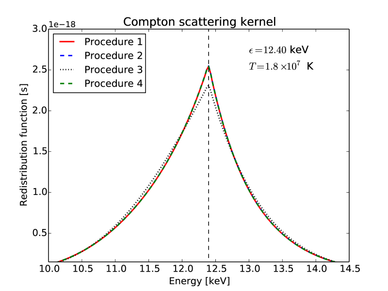
Figure 1: Angle-integrated Compton scattering redistribution functions for X-ray photons of initial wavelength $\lambda=1\AA$ (initial energy $\epsilon=12.4$ keV) in gas of electron temperatures $T=1.8\times 10^{7}$K. Note, that the formulae by Guilbert (1981) predict practically the same Compton redistribution function as the exact quantum-mechanical formulae by Suleimanov et al. (2012), compare the solid red line and dashed blue line. The approximate formulae by Arutyunyan and Nikogosyan (1980) yield a slightly different function, see the black dotted line. Green dashed line results from RF by Sazonov and Sunyaev (2000) and matches the exact RF.

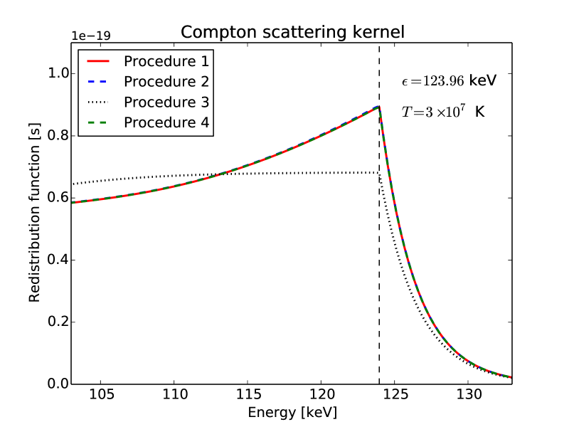
Figure 2: Angle-integrated Compton scattering redistribution functions for X-ray photons of initial wavelength $\lambda=0.1\AA$ (initial energy $\epsilon=124$ keV) in a gas of electron temperature $T=3\times 10^{7}$K. Again, the formulae by Guilbert (1981) and Sazonov & Sunyaev (2000) yield practically the same Compton RF as the exact quantum-mechanical formulae by Suleimanov et al. (2012). The black dotted line denote the approximate RF obtained from Arutyunyan and Nikogosyan (1980).

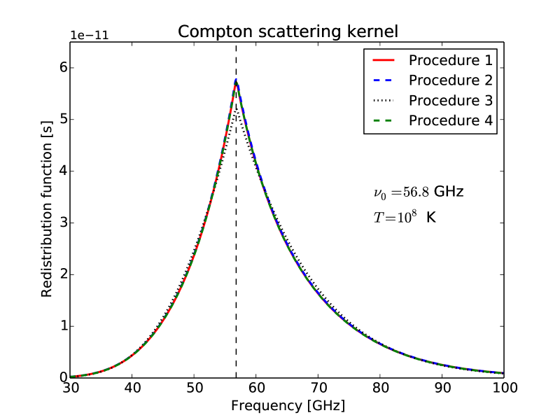
Figure 3: Angle-integrated Compton scattering redistribution functions for microwave photons of initial frequency $\nu=56.8$ GHz, corresponding to a radiation temperature 2.768 K. Soft photons are scattered here in the hot intra-cluster gas of electrons at temperature of $T=10^{8}$K. All the redistribution functions show the inverse Compton scattering effect. Again RF’s by Guilbert (1981), Suleimanov et al. (2012), and Sazonov & Sunyaev (2000) are practically identical, compare the solid red line with the overlapping blue and green dashed lines.

7 Numerical results

Figures 1-5 present runs of the angle-integrated redistribution functions $R_{i}(\nu,\nu^{\prime})$ computed for a few sample gas temperatures and initial photon energies. Note, that functions $R_{i}(\nu,\nu^{\prime})$ are given always in Hz^-1, while photon energies are either in keV or GHz (horizontal axis).

In all the figures, the redistribution function $R_{2}$ by Guilbert (1981) was drawn as a blue dashed line, while the exact function $R_{1}$ by Suleimanov et al. (2012) is represented by a red solid line. The shape and comparison of both redistribution functions for various assumed parameters is the most important part of this paper. Curves showing the approximate functions $R_{3}$ and $R_{4}$ were indicated for completeness (black dotted line and green dashed line, respectively).

Figs. 1-2 present the Compton redistribution functions for sample temperatures $T=1.8\times 10^{7}$ and $10^{8}$ K, which are typical for photospheres and envelopes of hot X-ray bursting neutron stars. The initial photon energy is similar to the energy of peak flux in the outgoing spectra (Fig. 1) or is a few times higher (Fig. 2). Both functions $R_{1}$ and $R_{2}$ are practically identical and overlap each other in the figures. Note, that in both cases reddening of the scattered X-ray photons apparently dominates over the blue-shift.

Fig. 3 illustrates the Compton scattering of microwave photons of cosmic background radiation (CMB) of the temperature $T=2.768$ K, scattered in hot gas in galaxy clusters of $T=10^{8}$. Also here both functions $R_{1}$ and $R_{2}$ are identical. All the functions $R_{1}-R_{4}$ reproduce the inverse Compton effect and the blue-shift of microwave photons dominates.

Fig. 4 demonstrates trace differences between both the essential redistribution functions $R_{1}$ and $R_{2}$ for hard X-rays at temperature $T=10^{8}$ K, which corresponds to the deepest layers of hot neutron star atmospheres. More substantial differences appear only at $T=10^{9}$ K or higher. As the example, Fig. 5 shows the Compton redistribution functions for gamma ray photons of energy 1.24 MeV, significantly exceeding the energy of the electron rest mass (511 keV).

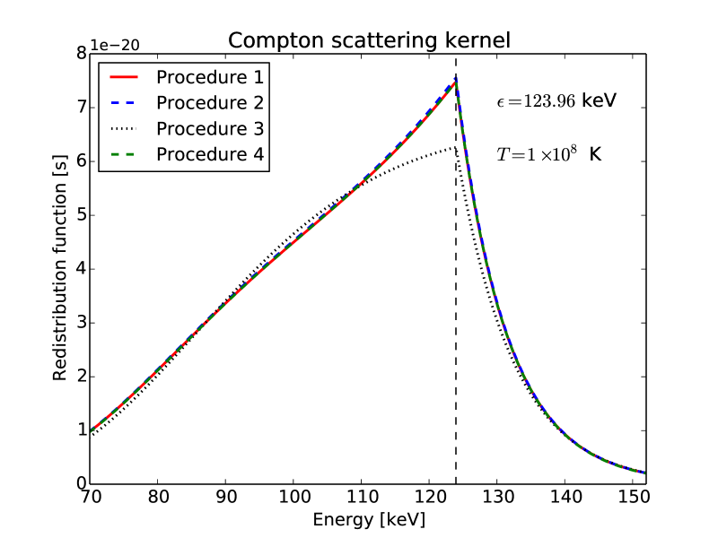
Figure 4: Angle-integrated Compton scattering redistribution functions for X-ray photons of initial wavelength $\lambda=0.1\AA$ (initial energy $\epsilon=124.$ keV) in a gas of electron temperature $T=10^{8}$K. Formulae by Guilbert (1981) and Sazonov & Sunyaev (2000) predict marginally different Compton redistribution function than the quantum mechanical formulae, compare the solid red line and the dashed blue and dashed green lines.

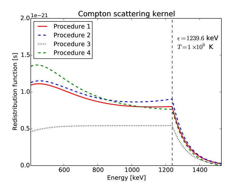
Figure 5: Angle-integrated Compton scattering redistribution functions for X-ray photons of initial wavelength $\lambda=0.01\AA$ (initial energy $\epsilon=1.24$ MeV) in a gas of electron temperature $T=10^{9}$K. Only at such high $T$ do the exact Compton scattering redistribution function (solid red line) markedly differ from Guilbert’s (1981) and Arutyunyan and Nikogosyan (1980) values.

7.1 Thermodynamic equilibrium

Compton scattering redistribution function must obey the symmetry relation, valid for electrons of maxwellian velocity distribution in thermodynamic equilibrium (Pomraning 1973, Eqs. 8.1-8.2). The relation can be written as

$$\Delta(\epsilon,\epsilon_{1},\eta,\Theta)=R_{i}(\epsilon,\epsilon_{1},\eta)\epsilon^{2}\exp(-\epsilon/\Theta)-R_{i}(\epsilon_{1},\epsilon,\eta)\epsilon_{1}^{2}\exp(-\epsilon_{1}/\Theta)=0\,.$$ (27)

We numerically verified that equation for all Compton redistribution functions $R_{i}$, $i=1,\ldots,4$ and computed tables of relative differences $\Delta_{i}/R_{i}$ for all temperatures, initial energies $\epsilon$ and energy ranges $\epsilon^{\prime}$ shown in Figs. 1-5 and the cosine of scattering angles in the full range [-1,+1]. The above identity was numerically reproduced here for $R_{1}$, $R_{2}$ and $R_{3}$ with the relative difference less than $10^{-19}$ (absolute value) almost everywhere in the parameter space, except at $\eta\rightarrow+1$, where the relative difference could rise above $10^{-7}$.

Therefore, we conclude that the Guilbert’s redistribution function $R_{2}$ described here fulfils the detailed balance condition.

8 Summary

This paper presents four alternative formulae for calculating the photon redistribution function specific for the Compton scattering of unpolarized light. Our considerations are valid in a perfect gas of electrons with isotropic relativistic thermal velocities. These formulae were derived from published papers on Compton scattering.

The final scattering redistribution functions $R_{i}(\nu,\nu^{\prime},\eta)$, $i=1,\ldots,4$, are presented here in a unified dimensional form, which are ready to use in radiative transfer calculations ($i=1$ or 2). Approximate algorithms No. 3-4 should not be used in accurate model atmosphere calculations.

Furthermore, we present for the first time the correct set of equations defining the Compton redistribution function ($R_{2}$) derived by Guilbert (1981). The original paper was published with computational errors making his results essentially useless. That method, now using correct equations, was applied in the original Fortran code for model atmosphere computations of X-ray bursting neutron stars (Madej 1991a,b; Madej et al. 2004).

We present also the exact quantum mechanical redistribution function $R_{1}$ (see Section 3), defined in detail in Suleimanov et al. (2012). We derived a new expression for $R_{2}$ by algebraic manipulation of the equations given in their paper, which allowed us to perform numerical computations of $R_{2}$ in a wide range of photon energies, from gamma rays down to radio waves. Note, that our formulae are ideally suited for study of both hot stellar atmospheres and spectral distortions of the cosmic microwave radiation (Sunyaev-Zel’dovich effect), see Sazonov & Sunyaev (1998), Chluba et al. (2012) and Chluba & Dai (2014).

Some sample angle-integrated Compton scattering redistribution functions in hot plasma were computed for gas temperatures $10^{7}\leq T\leq 10^{9}$ K and initial photon energies differing by many orders of magnitude. The resulting Figures 1-5 show that both algorithms by Guilbert (1981) and the exact quantum mechanical equations produce the same redistribution functions, $R_{1}$ and $R_{2}$, for Compton scattering in plasma at a temperature $T\leq 10^{8}$ K. These are the typical temperatures that occur in the atmospheres of X-ray bursters and intracluster plasma. Only for higher temperatures, $T\geq 10^{9}$ K, do both curves start to come apart.

The Fortran 77 computer code for computations of all four Compton redistribution functions, $R_{1}$ to $R_{4}$, can be found at http://www.astrouw.pl/~jm/software.html.

9 Appendix A

Guilbert (1981) defined the probability of scattering a photon of energy $\epsilon$ to energies between $\epsilon_{1}$ and $\epsilon_{1}+d\epsilon_{1}$, from a direction ${\bf n}$ into a solid angle $d\Omega_{1}$, in a direction ${\bf n_{1}}$ along the raypath $dr$ is given by:

$$P\,d\epsilon_{1}\,d\Omega_{1}\,dr=\int\int(1-\beta\cdot{\bf n}){{d\sigma}\over{d\Omega_{1}}}M(\beta){{\partial\beta}\over{\partial\epsilon_{1}}}d\epsilon_{1}d\Omega_{1}dr.$$ (28)

Energies are in units of the electron rest mass, $m_{e}c^{2}$; $\beta$ is the electron velocity in units of the speed of light; $M(\beta)$ is the electron velocity distribution and ${d\sigma}/{d\Omega_{1}}$ is the differential cross-section for Compton scattering.

$$(1-\beta\cdot{\bf n}){{d\sigma}\over{d\Omega_{1}}}={{3\sigma_{T}}\over{16\pi}}{{\bar{X}}\over({1-\beta\cdot{\bf n}})}{1\over\gamma^{2}s^{2}}$$ (29)

$$\bar{X}\equiv 2-2\left[1-{\epsilon^{2}\over 2s}(1-\cos{\theta})\right]{{1-\cos{\theta}}\over{\gamma^{2}(1-\beta\cdot{\bf n})(1-\beta\cdot{\bf n_{1}})}}+\left[{{1-\cos{\theta}}\over{\gamma^{2}(1-\beta\cdot{\bf n})(1-\beta\cdot{\bf n_{1}})}}\right]^{2}$$ (30)

where

$$s\equiv\epsilon/\epsilon_{1};\,\,\,\,\,\,\,\,\cos{\theta}={\bf n}\cdot{\bf n_{1}};\,\,\,\,\,\,\,\,\gamma={1\over(1-\beta^{2})^{1/2}}$$

(see Babuel-Peyrissac & Rouvillois 1969).

For Compton scattering we have:

$${1\over s}={{1-\beta\cdot{\bf n}}\over{\epsilon\gamma^{-1}(1-\cos{\theta})+1-\beta\cdot{\bf n_{1}}}},$$ (31)

or, by rearranging terms

$$\beta\cdot({\bf n_{1}}-s\,{\bf n})=1-s-\epsilon\gamma^{-1}(1-\cos{\theta})$$ (32)

The above set of equations was transformed by Guilbert (1981) to

$$P(\epsilon,s,\theta,x)=-{3\over{64\pi^{2}}}\,{1\over{Es^{2}}}\,{x\over{K_{2}(x)}}\int\limits_{\gamma_{\rm min}}^{\infty}F(\epsilon,\epsilon_{1},\theta,\gamma)\,\exp(-\gamma/\Theta)\,d\gamma\,,\\$$ (33)

where the dimensionless gas temperature $x=m_{e}c^{2}/{kT}$ Other auxiliary variables are defined as

$$A = 1-s\,,\hskip 28.45274ptB=\epsilon(1-\cos\theta)\,,\hskip 28.45274ptE=(1-2s\cos\theta+s^{2})\,^{1/2}\,,$$ (34)

$$\gamma_{\rm min} = \left\{\left[{E^{2}\over{E^{2}+B^{2}}}\left(1-{A^{2}\over{E^{2}+B^{2}}}\right)\right]^{1/2}-{AB\over{E^{2}+B^{2}}}\right\}^{-1}\,.$$ (35)

Relativistic Compton redistribution function then equals to

$$F(\epsilon,\epsilon_{1},\theta,\gamma)=(1-\beta_{z})\int\limits_{0}^{2\pi}{{\bar{X}}\over({1-\beta\cdot{\bf n}})}\,d\phi\,,\hskip 42.67912pt{\rm where}\>\>\>\beta_{z}=(A+B\gamma^{-1})/E\,.$$ (36)

Function $F(\epsilon,s,\theta,\gamma)$ can be expressed by the trinomial (Guilbert 1981)

$$F(\epsilon,s,\theta,\gamma)=2aI_{1}+{2a\over\gamma^{2}}(1-\cos\theta)\left[1-{\epsilon^{2}\over 2s}(1-\cos\theta)\right]I_{2}+{a\over\gamma^{4}}(1-\cos\theta)^{2}I_{3},$$ (37)

Let us define variables

$$a = 1-(\cos\theta-s)\,{1-s+\epsilon\,(1-\cos\theta)/\gamma\,\over{1-2s\cos\theta+s^{2}}}$$ (38)

$$b = -\left({\gamma^{2}-1\over\gamma^{2}}-{(1-s+\epsilon(1-\cos\theta)/\gamma)^{2}\over{1-2s\cos\theta+s^{2}}}\right)^{1/2}\left({1-\cos^{2}\theta\over{1-2s\cos\theta+s^{2}}}\right)^{1/2}$$ (39)

$$c = 1-(1-s\cos\theta)\,{1-s+\epsilon\,(1-\cos\theta)/\gamma\,\over{1-2s\cos\theta+s^{2}}}$$ (40)

$$d = b\,s$$ (41)

$$y = {b\over\sqrt{a^{2}-b^{2}}}+{d\over\sqrt{c^{2}-d^{2}}}$$ (42)

then the partial integrals

$$I_{1} = {{2\pi}\over\sqrt{a^{2}-b^{2}}}$$ (43)

$$I_{2} = {{2\pi}\over{y(a^{2}-b^{2})^{2}(c^{2}-d^{2})}}\left[a(bc+ad)+b(ac+bd)-{{ab(bc+ad)}\over{y\sqrt{a^{2}-b^{2}}}}\right]$$ (44)

$$I_{3} = {{\pi}\over{y(a^{2}-b^{2})^{3}(c^{2}-d^{2})^{2}}}~{}\times~{}\left(~{}\left[a(bc+ad)+b(ac+bd)-{{ab(bc+ad)}\over{y\sqrt{a^{2}-b^{2}}}}\right]\right.$$

$$\times \left.\left[{{2abcd}\over{y^{2}\sqrt{a^{2}-b^{2}}\sqrt{c^{2}-d^{2}}}}-{{4acd}\over{y\sqrt{c^{2}-d^{2}}}}-{{2abc}\over{y\sqrt{a^{2}-b^{2}}}}+8ac\right]\right.$$

$$+ \left.\left[2ad+2bc-{{b^{2}c+2abd}\over{y\sqrt{a^{2}-b^{2}}}}+{{a^{2}b(bc+ad)}\over{y(a^{2}-b^{2})^{3/2}}}-{{a^{2}b^{2}(bc+ad)}\over{y^{2}(a^{2}-b^{2})^{2}}}\right]\times(a^{2}-b^{2})c\left({d\over{y\sqrt{c^{2}-d^{2}}}}-2\right)\right.$$

$$+ \left.\left[2ab-{{ab^{2}}\over{y\sqrt{a^{2}-b^{2}}}}-{{abcd(bc+ad)}\over{y^{2}\sqrt{a^{2}-b^{2}}(c^{2}-d^{2})^{3/2}}}\right]\times\left[{{ab(c^{2}-d^{2})}\over{y\sqrt{a^{2}-b^{2}}}}-4a(c^{2}-d^{2})\right]+2b(a^{2}-b^{2})(c^{2}-d^{2})\right.$$

$$- \left.{b^{2}\over y}\sqrt{a^{2}-b^{2}}(c^{2}-d^{2})-a^{2}b^{3}{{(c^{2}-d^{2})}\over{y^{2}(a^{2}-b^{2})}}+a^{2}b^{2}{{(c^{2}-d^{2})}\over{y\sqrt{a^{2}-b^{2}}}}-{{bcd(bc+2ad)}\sqrt{a^{2}-b^{2}}\over{y^{2}\sqrt{c^{2}-d^{2}}}}\right.$$

$$- \left.{{2a^{2}b^{2}cd(bc+ad)}\over{y^{3}(a^{2}-b^{2})\sqrt{c^{2}-d^{2}}}}+{{a^{2}bcd(bc+ad)}\over{y^{2}\sqrt{a^{2}-b^{2}}\sqrt{c^{2}-d^{2}}}}\right)$$

The above algorithm was defined by Guilbert (1981), who in his paper presented an erroneous expression for the integral $I_{3}$. Herein, we correctly define the coefficient $I_{3}$, which was used in a series of papers on model atmospheres of bursting neutron stars (Madej 1989, 1991a, 1991b).