Spin susceptibility and electron-phonon coupling of two-dimensional materials by range-separated hybrid density functionals: Case study of Li_xZrNCl

Abstract

We investigate the capability of density functional theory (DFT) to appropriately describe the spin susceptibility, $\chi_{s}$, and the intervalley electron-phonon coupling in Li_xZrNCl. At low doping, Li_xZrNCl behaves as a two-dimensional two-valley electron gas, with parabolic bands. In such a system, $\chi_{s}$ increases with decreasing doping because of the electron-electron interaction. We show that DFT with local functionals (LDA/GGA) is not capable of reproducing this behavior. The use of exact exchange in Hartree-Fock (HF) or in DFT hybrid functionals enhances $\chi_{s}$. HF, B3LYP, and PBE0 approaches overestimate $\chi_{s}$, whereas the range-separated HSE06 functional leads to results similar to those obtained in the random phase approximation (RPA) applied to a two-valley two-spin electron gas. Within HF, Li_xZrNCl is even unstable towards a ferromagnetic state for $x<0.16$. The intervalley phonons induce an imbalance in the valley occupation that can be viewed as the effect of a pseudomagnetic field. Thus, similarly to what happens for $\chi_{s}$, the electron-phonon coupling of intervalley phonons is enhanced by the electron-electron interaction. Only hybrid DFT functionals capture such an enhancement and the HSE06 functional reproduces the RPA results presented in M. Calandra et al. [Phys. Rev. Lett. 114, 077001 (2015)]. These results imply that the description of the susceptibility and electron-phonon coupling with a range-separated hybrid functional would be important also in other two-dimensional weakly doped semiconductors, such as transition-metal dichalcogenides and graphene.

I Introduction

Low doping of layered multivalley semiconductors is a field of intense research in nanotechnology and superconductivity Saito et al. (2015); Lu et al. (2015). Fairly high T_c values have been reported with doped two-dimensional semiconductors, such as transition metal dichalcogenides Novoselov et al. (2005); Xu et al. (2014); Zhang et al. (2014); Ye et al. (2012); Lu et al. (2015), ternary transition-metal dinitrides Gregory et al. (1998), and cloronitrides Yamanaka et al. (1996, 1998); the doping of which can be achieved and controlled by intercalation Yamanaka et al. (1996, 1998); Taguchi et al. (2006); Takano et al. (2008a, b); Yamanaka et al. (2009) or field effect Novoselov et al. (2005); Xu et al. (2014); Ye et al. (2010); Kasahara et al. (2011); Brumme et al. (2014); Saito et al. (2015).

Weakly doped two-dimensional, and quasi-two-dimensional (2D) semiconductors composed of weakly interacting layers stacked along the $z$-direction, behave very differently than their 3D counterparts. In 3D semiconductors, with parabolic bands, the density of states, $N(0)$, increase as the square root of the Fermi level, so that the number of electrons increases smoothly from zero. This explains why a substantial number of carriers needs to be inserted in 3D semiconductors to achieve superconductivity Ekimov et al. (2004). In a phonon-mediated mechanism, T_c is often proportional to the density of states at the Fermi level. In 2D, as the density of states (DOS) is constant, one would expect a constant $T_{c}$ as long as the phonon spectrum is weakly affected by doping.

This is in stark contrast with what happens in Li_xZrNCl in the low doping limit. This layered system can be considered the prototype of 2D 2-valley electron gas. Indeed the bottom of the conduction band of ZrNCl is composed of two perfectly parabolic bands at points ${\bf K}$ and ${\bf K^{\prime}}=2{\bf K}$ in the Brillouin zone. The interlayer interaction is extremely weak Heid and Bohnen (2005); Takano et al. (2011); Botana and Pickett (2014); Calandra et al. (2015). Upon Li intercalation, the semiconducting state is lost and superconductivity emerges. Surprisingly, the superconducting critical temperature $T_{c}$ is strongly enhanced in the low-doping limit Yamanaka et al. (1996, 1998); Taguchi et al. (2006), despite essentially parabolic bands, two-valley electronic structure and an almost constant DOS Heid and Bohnen (2005); Takano et al. (2011); Botana and Pickett (2014).

In a 2D 2-valley electron gas, the reduction of doping implies an increase of the $r_{s}$ electron-gas parameter and, consequently, of the electron-electron interaction Giuliani and Vignale (2005). Then it can be expected that in the low doping limit the electronic structure, the vibrational properties, and the electron-phonon interaction are strongly affected. This is confirmed by the behavior of the magnetic susceptibility. Despite Li_xZrNCl being nonmagnetic, in the low-doping limit, the magnetic susceptibility is enhanced in a way very similar way to that in the superconducting T_c. The interacting magnetic susceptibility $\chi_{s}$ is not constant, and strongly deviates from the constant free-electron-like behavior in 2D Kasahara et al. (2009); Taguchi et al. (2010); in particular, the susceptibility $\chi_{s}$ is enhanced at the low-doping regime.

In a previous workCalandra et al. (2015), the behavior of $\chi_{s}$ and $T_{c}$ as a function of doping was investigated by using local functionals and a 2D two-valley electron gas model solved within the random phase approximation (RPA). In this framework, it was found that the electron-electron interaction enhances the electron-phonon matrix elements of those intervalley phonons inducing an unbalance in the valley occupations. The enhancement increases by increasing the $r_{s}$ parameter or, equivalently, by decreasing the electron density.

In this paper, we perform a systematic study of electronic, magnetic, and vibrational properties of Li_xZrNCl using density functional theory (DFT) beyond the standard LDA/GGA approximations. We investigate the effect of an exact exchange component on these properties and discuss the relevance of electron-electron interaction in determining the superconducting properties of Li_xZrNCl.

In the following section, we show the structures used in our calculations. In Sec. III, we present the technical details of our calculations. In Sec. IV, we present the results of the electronic structure, magnetic properties of valley and spin susceptibility, phonon frequencies, and electron-phonon coupling. In the final section, we conclude our work.

II Crystal Structure

The structures of undoped $\beta$-ZrNCl and Li-doped ZrNCl have been investigated using synchrotron x-ray Chen et al. (2001); Taguchi et al. (2006) and powder neutron diffraction Shamoto et al. (1998). The primitive unit cell of ZrNCl has rhombohedral structure (space group $R\bar{3}m$, number $166$) with 2 formula units per unit cell. It can be also be constructed by a conventional cell of hexagonal structure with 6 formula units per cell, as shown in Fig. 1, where the ABC layer stacking is evident.

Upon Li intercalation, Li atoms are placed between the ZrNCl layers. Li acts as a donor and gives electrons to the Zr-N layers. It has been shown that the Li intercalation can be simulated by including an effective background charge, both for what concerns the electronic structure and the phonon dispersion Heid and Bohnen (2005); Botana and Pickett (2014). Thus, we simulate Li doping by changing the number of electrons and using a compensating jellium background. In all our calculations, the lattice parameters $a$ and $c$ are fixed to experimental values of each doping Shamoto et al. (1998); Chen et al. (2001); Taguchi et al. (2006) and the atomic coordinates are relaxed within a fixed volume.

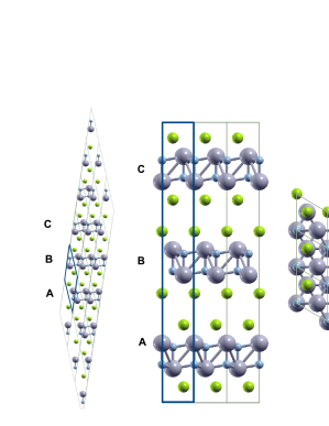
Figure 1: ZrNCl structure. Left: Rhombohedral cell repeated $3a\times 3b\times 3c$ to show the stacking. The unit cell with 2 formula units is highlighted. Middle: Hexagonal conventional cell repeated $3a\times 3a\times c$ to show the stacking with the side view along $\hat{a}-\hat{c}$ plane. The conventional unit cell with 6 formula units is highlighted. Right: Top view along $\hat{a}-\hat{b}$ plane.

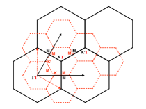
Figure 2: Brillouin zone of the hexagonal lattice of ZrNCl. Large solid black hexagons represent the unit cell and small dashed red hexagons represent the $\sqrt{3}\times\sqrt{3}\times 1$ supercell. Note that the K and K’ of the unitcell fold onto the $\Gamma$ point of the supercell.

In order to be able to carry out the finite-difference electron-phonon coupling calculation at the special point ${\bf K}$, we take advantage of the weak interaction between the layers Kasahara et al. (2010), making the stacking order negligible. Therefore, we adopt the ZrNCl structure with the lattice parameter $a$ set to the experimental value of each doping and simulate a single layer by inserting 12.5 Å vacuum between one ZrNCl layer and its periodic image corresponding to $c=18.734$ Å. This is equivalent to the hexagonal structure with the space group $P\bar{3}m1$ (space group number 164), with 2 formula units in the unit cell. Then we create a supercell with the lattice vectors $\sqrt{3}a\times\sqrt{3}a\times c$, with 6 formula units. In the Brillouin zone associated with the $\sqrt{3}\times\sqrt{3}\times 1$ supercell of the hexagonal structure, the special points ${\bf K}$ and ${\bf K^{\prime}}$ fold at ${\bf\Gamma}$, as shown in Fig. 2.

III Computational Details

Calculations are performed using the Hartree-Fock (HF) approximation and various flavors of DFT: the Perdew-Zunger parametrization of the local density approximation (LDA) Dirac (1930); Perdew and Zunger (1981) , and generalized gradient approximation (GGA) as implemented in PBE Perdew et al. (1996); hybrid functionals with different exact exchange components, i. e., B3LYP Becke (1993); Lee et al. (1988); Vosko et al. (1980) and PBE0  Adamo and Barone (1999); and the range-separated HSE06  Krukau et al. (2006) hybrid functional. The CRYSTAL14 periodic ab initio code Dovesi et al. (2014a) is used with norm-conserving pseudopotentials and Gaussian-type triple-$\zeta$ valence polarized basis sets Weigend and Ahlrichs (2005) with the most diffuse Gaussian functions of the Zr basis set reoptimized for periodic calculations. In order to check the accuracy of the Gaussian basis sets, the electronic band structure is compared to that obtained from a plane wave basis set calculation performed using the Quantum ESPRESSO method Giannozzi et al. (2009) with the PBE functional Perdew et al. (1996).

The doping of the semiconductor is simulated by changing the number of electrons on a compensating jellium background, which has been previously shown to give accurate results for this system Heid and Bohnen (2005); Botana and Pickett (2014). The atomic coordinates are relaxed with lattice parameters fixed at the experimental values. For the energy convergence, a tolerance on the change in total energy of $10^{-9}$ Ha is used for all calculations. A Fermi-Dirac smearing of 0.0025 Ha; shrinking factors of 48-48, corresponding to an electron-momentum grid of $48\times 48\times 48$; and real space integration tolerances of 7-7-7-15-30 are used for the relaxation of the internal coordinates and calculating the electronic band structure Dovesi et al. (2014b). With this method, the exact exchange is computed in direct space, so the $k$ grids and $q$ grids of the electron momentum for the functionals with the exact exchange are equivalent. The density of states is calculated using a Gaussian smearing of 0.005 Ha.

The effective mass, $m^{*}$ is calculated from the curvature of a fourth order polynomial fit to the region between the Fermi energy and the conduction band minimum around the special point, K, assuming that the mass tensor is isotropic. The fit parameters are given in Appendix A.

The spin susceptibility, $\chi_{s}$, obtained from the curvature of the energy as a function of total magnetization, $M$, is more sensitive to the smearing and the $k$ grid. Therefore, a smaller Fermi-Dirac smearing temperature of 0.00125 Ha and finer shrinking factors of 120-120 are used to obtain energy as a function of magnetization, $E(M)$.

Electron-phonon coupling matrix elements and phonon frequencies are calculated with Fermi-Dirac smearing of 0.0035 Ha and shrinking factors of $24\times 24\times 1$ in the $\sqrt{3}\times\sqrt{3}\times 1$ supercell of a single 2D lattice with AAA stacking. The bands with the HF approximation in Sec. IV.2 are also plotted with these parameters. For the electron-phonon coupling calculations, the atoms are displaced according to the phonon pattern of the mode. As this pattern is determined only by symmetry, we use the same pattern as a function of doping.

IV Results

IV.1 Electronic Structure

Undoped $\beta$-ZrNCl is a large gap insulator. The direct band gap of the insulating compound is measured to be 3.4 eV with optical absorption spectra Ohashi et al. (1989), while the indirect band gap of the Na_0.42ZrNCl is measured to be 2.5 eV with valence-band photoemission Yokoya et al. (2004). When doped, Li intercalation acts as a rigid filling of the parabolic conduction band minima (valleys) at K and $\mathbf{K^{\prime}}=2\mathbf{K}$ of the Brillouin zone, leading to two quasispherical Fermi surfaces. We have calculated the electronic band structure with different levels of approximations to evaluate the effect of the exact exchange on the electronic structure, band gap, and effective mass.

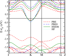
Figure 3: Electronic structure of Li_xZrNCl at doping $x=1/18$ with different functionals. The Fermi level is set to 0 eV. HF stands for Hartree-Fock.

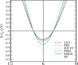
Figure 4: A detailed view of the electronic structure of Li_xZrNCl at doping $x=1/18$ around the conduction band minimum. The Fermi level is set to 0 eV.

The calculated electronic band structure is shown in Fig. 3 and a detailed view around the conduction band minimum is shown in Fig. 4 for the lowest calculated doping of $x=1/18$. Our PBE band structure is in agreement with previous calculations Botana and Pickett (2014). We also present the density of states of the undoped structure in Fig. 5. The fundamental band gap is between the $\Gamma$-point and the $\mathbf{K}$-point. We have also calculated the change in the direct band gap at the $\mathbf{K}$-point with different approximations. These results are presented in Fig. 6.

The LDA and PBE approximations produce similar results; the electronic bands and the density of states are almost indistinguishable. As a percentage of exact exchange is introduced with B3LYP and PBE0 functionals, the band gap increases with increasing exchange fraction. This becomes extreme in the HF limit, with a much larger band gap. Therefore, there is a clear trend on how the electronic structure is modified with introduction of the exact exchange in the approximations: the larger the exact exchange is, the larger is the calculated band gap. For example, for the lowest doping of $x=1/18$, the calculated band gap changes as follows: with LDA and PBE $E_{g}\sim 1.8$ eV, with B3LYP and PBE0 $E_{g}=2.8$ eV and $E_{g}=3.0$ eV respectively, and finally with HF (which is the most extreme case) $E_{g}=8.1$ eV. However, the introduction of the range separation together with the exact exchange breaks this pattern. With the HSE06 functional, we obtain a gap that is in between the PBE and B3LYP results. For the lowest doping of $x=1/18$, the calculated band gap becomes $E_{g}=2.6$ eV, and the HSE06 results are in very good agreement with the valence-band photoemission measurement of the indirect band gap of $E_{g}=2.5$ eV.

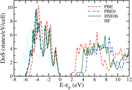
Figure 5: Density of states of undoped $\beta$-ZrNCl, with Fermi level set to the top of the valence band. The bottom of the conduction band has a quasiconstant density of states, a fingerprint of the 2D parabolic character of the electronic structure.

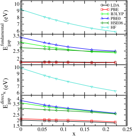
Figure 6: Change in the fundamental band gap with HF approximation (top panel) and DFT functionals (second panel), and in the direct band gap at the $\mathbf{K}$ point with HF approximation (third panel) and DFT functionals (bottom panel) as a function of doping with different approximations.

Furthermore, how the band gap changes with increasing doping is different with different approximations. The band gap essentially does not change in LDA and PBE approximations, with a decrease of $<0.02$ eV between the lowest and the highest doping. However, in the same doping range, the gap decreases by 0.4 eV for B3LYP and 0.5 eV for PBE0. The most extreme difference of $\sim$ 2 eV is obtained again with the HF approximation. Hence, the gap does not stay constant if the exact exchange is introduced. When the range separation is introduced, the band gap still decreases with the increasing doping, but the difference is in between the PBE and B3LYP functionals. With the HSE06 functional, the gap decreases by $\sim$ 0.2 eV between the lowest and highest doping, keeping the results in good agreement with the experimentally reported value.

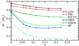
Figure 7: Change in the effective mass, $m^{*}$ as a function of doping with different approximations.

Another result we can deduce from the electronic band structure is the change in the curvature of the conduction band, from which the effective mass, $m^{*}$, is calculated. At fixed doping, as the exact exchange is introduced, the curvature of the conduction band gets larger, leading to smaller effective mass. This is also apparent in Fig. 4, and can be seen when the PBE functional is compared to the hybrid B3LYP functional, and further to the PBE0 functional. Intermediate steps of the B3LYP functional with the percentage of exact exchange changed to 5$\%$ and 10$\%$ can be found in Appendix B, and a gradual change in the effective mass and the band gap is observed. The next step is introducing the range separation using the HSE functional family. When the range separation of this functional is set to zero, i.e., $\omega=0$ Bohr^-1, the PBE0 functional is recovered. As the range separation parameter is increased to an intermediate value of $\omega=0.055$ Bohr^-1, the curvature starts to get smaller again, resulting in increasing the effective mass. This is also presented in Appendix B. The HSE06 functional with range separation $\omega=0.11$ Bohr^-1 further increases the effective mass, giving a value between the PBE and B3LYP functionals. The exact results are in Table 2. The experimental value of the effective mass is 0.9 $m_{e}$ Takano et al. (2011); however, this is an indirect derivation of the effective mass obtained from the optical reflectivity spectra using the Drude model, and its value deviates from our HSE06 calculations.

The change in the $m^{*}$ as a function of doping is shown in Fig. 7. While the change in the effective mass as a function of doping is almost constant for PBE and LDA functionals, the introduction of the exact exchange with the B3LYP and PBE0 functionals shows a difference of $\sim 0.15$ m_e between the undoped $x=0$ and the lowest doped $x=1/18$ cases. This difference is more dramatic with the HF approximation: the effective mass is too small even in the undoped case and goes further down upon doping. Finally, the HSE06 functional displays only a moderate decrease with increasing doping.

IV.2 Spin and Valley Magnetic Fields and Instabilities with the HF Approximation

As shown in the previous section, the electronic structure of Li_xZrNCl is composed by two parabolic bands (valleys) at points ${\bf K}$ and ${\bf K^{\prime}}$ in the Brillouin zone. By adopting AAA stacking and an in-plane $\sqrt{3}\times\sqrt{3}\times 1$ supercell, the special ${\bf K}$ and ${\bf K^{\prime}}$ of the unit-cell Brillouin-zone fold at ${\bf\Gamma}$ in the Brillouin zone of the supercell. As a result, there will be two perfectly degenerate parabolic bands at ${\bf\Gamma}$ in the supercell Brillouin zone. By including the spin degrees of freedom, the total degeneracy at ${\bf\Gamma}$ of the supercell Brillouin zone is $4$.

The nonmagnetic electronic structure calculated with the HF approximation and plotted in the $\sqrt{3}\times\sqrt{3}\times 1$ Brillouin zone is shown in Fig. 8 (a). If a spin unbalance is allowed (i. e., a finite magnetization), then the spin degeneracy is broken and each one of the two bands splits in two twofold-degenerate bands [see Fig. 8 (b)]. In the Brillouin zone of the unit cell, this would mean that the spin degeneracy in the valleys at ${\bf K}$ and ${\bf K^{\prime}}$ is broken in the same way, as these two special points are still equivalent due to the unbroken $C_{6}$ symmetry.

Within the HF approximation, as a finite magnetization is introduced to the system, the energy goes down, signifying that the HF approximation favors the magnetic state as the ground state. For $x=1/18$, the energy of the undistorted system under magnetization in Fig. 8 (b) is 88 meV/cell (6 formula units) lower than the undistorted and nonmagnetic system in Fig. 8 (a). This region of instability with the HF approximation continues up to the doping $x=1/6$, as will be discussed in the following section.

It has been shown in Ref. Calandra et al., 2015 that all phonons strongly coupled to electrons and having phonon momentum ${\bf q}={\bf K},{\bf K^{\prime}}$ (intervalley phonons) act as pseudo-magnetic fields, namely induce an asymmetry in the valley occupation, without breaking the spin degeneracy, at least as long as there is no net magnetization. Thus the intervalley distortion shifts the two valleys, changes the occupation per valley but preserves the absence of a magnetization in each valley. The action of an intervalley phonon on the electronic structure at zero magnetization is shown in Fig. 8 (c).

Within the HF approximation, as the atoms are distorted along a phonon mode, the energy goes down; signifying that the HF approximation favors the charge density state as the ground state. For $x=1/18$, the energy of the distorted and nonmagnetic system in Fig. 8 (c) is 101 meV/cell (6 formula units) lower than the undistorted and nonmagnetic system in Fig. 8 (a).

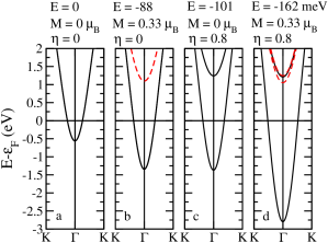
Figure 8: Electronic bands with HF approximation with $\sqrt{3}\times\sqrt{3}\times 1$ cell at doping $x=1/18$. (a) Undistorted phase, with the displacement prefactor, $\eta=0$ [see Eq. (6)]; no magnetization $M=0$. (b) Undistorted phase under magnetization. (c) Distorted phase, no magnetization. (d) Distorted phase under magnetization. The bands in (b) and (c) are obtained at the energy minimum of the $E(M)$ and $E(\eta)$ curves, respectively. The difference between the energy of the structure in (a) and other structures is given in meV/cell (6 formula units) above each figure. The splitting between the two topmost bands in (d) is $\sim$ 0.03 eV. Red dashed lines represent the minority spin and black solid lines represent the majority spin. The Fermi levels are shown by the black solid horizontal lines.

Finally, Fig. 8 (d) shows the combined effect of an intervalley distortion and a finite magnetization. The fourfold degeneracy at ${\bf\Gamma}$ in the Brillouin zone of the supercell is completely broken and $4$ different bands appear with different spin and electron occupations.

As expected, with the HF approximation, the distorted magnetic state has a lower energy than the undistorted non-magnetic state. For $x=1/18$, the energy of the distorted and magnetic system in Fig. 8 (d) is 162 meV/cell (6 formula units) lower than the undistorted and nonmagnetic system in Fig. 8 (a).

IV.3 Spin Susceptibility

Magnetic properties are described by the spin susceptibility, which is the response of the spin magnetization to an applied magnetic field, namely:

$$\chi_{s}=\left(\frac{\partial^{2}E}{\partial M^{2}}\right)^{-1}$$ (1)

where $E$ and $M$ are the total energy and magnetization, respectively.

The non interacting spin susceptibility, $\chi_{0s}$, is obtained by neglecting the electron-electron interaction of the conducting electrons. For perfectly parabolic bands, the non interacting spin susceptibility is doping independent and equal to

$$\chi_{0s}=\mu_{s}N(0)=\frac{g_{v}m^{*}}{\pi\hbar^{2}}$$ (2)

where $\mu_{s}$ is the Bohr magneton, $g_{v}$ is the valley degeneracy ($2$ in our case), and $m^{*}$ the band effective mass. We calculate $\chi_{0s}$ from the density of states of the undoped compound, which is shown in Fig. 5, and by extrapolating the $N(0)$ of the desired doping. Our calculations show that $\chi_{0s}$ is not enhanced at the low-doping limit.

Experimental measurements Kasahara et al. (2009); Taguchi et al. (2010) carried out on Li_xZrNCl show that (i) the system is not magnetic and (ii) the spin susceptibility in Li_xZrNCl is strongly doping dependent with a marked enhancement in the low-doping limit Kasahara et al. (2009); Taguchi et al. (2010), which is different than the expected $\chi_{0s}$ behavior. It is then natural to look for exchange and correlation effects in the susceptibility.

We calculate the spin susceptibility with local and hybrid functionals by finite differences. Namely we calculate the total energy at fixed magnetization and then use Eq. (1) to obtain $\chi_{s}$.

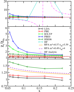
Figure 9: Magnetic susceptibility enhancement factor, $\chi_{s}/\chi_{0s}$, obtained with different approximations. Each panel shows a detailed view of the panel above.

In Fig. 9, we present the spin susceptibility enhancement factor $\chi_{s}/\chi_{0s}$ as a function of doping with different approximations. The top panel of Fig. 9 displays the behavior of the enhancement factor with the HF approximation. The HF approximation predicts that the nonmagnetic state is unstable in the low-doping limit. As the magnetization is turned on, there is a finite gain in energy leading to a negative spin susceptibility, $\chi_{s}$. This result is in agreement with HF calculations carried out in multivalley 2D electron gas Marchi et al. (2009). Furthermore, we have analytically calculated the spin susceptibility enhancement with the HF approximation, considering the thickness of the 2D electron gas by including a form factor. Details of the analytic expressions are given in Appendix E. The region of instability with the analytic HF calculation is similar to the numerical results, proving that the form factor correctly takes into account the finite thickness of the 2D electron gas.

By reducing the amount of HF exchange in the functional, the spin susceptibility enhancement at low doping is reduced, as shown in Fig. 9. On the contrary, the bottom panel of Fig. 9 shows that the LDA and PBE approximations show hardly any spin susceptibility enhancement. Thus, the susceptibility enhancement is entirely due to the exchange interaction. In Fig. 9, we also compare our results with those obtained by a model based on RPA Zhang and Das Sarma (2005); Calandra et al. (2015) . The model assumes a 2D 2-valley electron gas with no intervalley Coulomb scattering. Under this assumption, only the intravalley electron-electron interaction remains and the RPA susceptibility can be calculated analytically, by using the LDA/PBE effective mass of undoped ZrNCl and the environmental dielectric constant, $\epsilon_{M}=5.59$ Takano et al. (2011); Botana and Pickett (2014); Kaur et al. (2010), used in Ref. Calandra et al., 2015. The model is appropriate in the low-doping limit where $|{\bf k_{F}}-{\bf K}|<<K$ (see Supplementary Material in Ref. Calandra et al., 2015), a condition necessary to have the intravalley electron-electron scattering dominating over the intervalley one.

As can be seen, the hybrid functional HSE06 gives an amount of enhancement from the high to low doping regime, comparable to the one obtained with the RPA model.

IV.4 Phonon Frequencies

In this section we evaluate the phonon frequencies of Li_xZrNCl as a function of doping for several functionals.

Table 1: Frequencies corresponding to the two modes at the K point with high electron-phonon coupling, and six modes at the $\Gamma$ point which are Raman active and compared to the experimental values. All the frequencies are given in cm^-1.

x	XC	K $\omega_{1}$	K $\omega_{2}$	$\Gamma$ A1g	$\Gamma$ A1g	$\Gamma$ A1g	$\Gamma$ Eg	$\Gamma$ Eg	$\Gamma$ Eg
0	Expt. [Ref. Adelmann et al., 1999]	$-$	$-$	187	326	590	123	179	604
0.16 ($\sim$1/6)	Expt. [Ref. Adelmann et al., 1999]	$-$	$-$	188	322	582	123	178	608
0	Expt. [Ref. Cros et al., 2003]	$-$	$-$	191	331	591	128	184	605
0	Expt. [Ref. Kitora et al., 2007]	$-$	$-$	198	336	600	$-$	191	614
0.06 ($\sim$1/18)	Expt. [Ref. Kitora et al., 2007]	$-$	$-$	198	336	601	$-$	190	614
0.10 ($\sim$1/9)	Expt. [Ref. Kitora et al., 2007]	$-$	$-$	197	331	592	$-$	185	620
0.14 ($\sim$1/6)	Expt. [Ref. Kitora et al., 2007]	$-$	$-$	197	324	583	$-$	181	613
0.24 ($\sim$2/9)	Expt. [Ref. Kitora et al., 2007]	$-$	$-$	195	326	585	$-$	181	613
0.31 ($\sim$1/3)	Expt. [Ref. Kitora et al., 2007]	$-$	$-$	190	323	577	$-$	178	603
0	LDA	595	252	187	336	591	128	191	580
1/18	LDA	484	227	186	332	587	127	188	584
1/15	LDA	483	225	186	331	586	127	188	585
1/12	LDA	483	220	186	330	584	126	187	587
1/9	LDA	485	215	186	328	581	126	187	589
1/6	LDA	498	203	184	323	574	123	185	593
2/9	LDA	505	195	182	316	564	118	182	597
0	PBE	589	243	176	322	568	120	176	573
1/18	PBE	484	219	176	318	563	118	174	578
1/15	PBE	482	216	176	317	563	118	174	579
1/12	PBE	481	211	176	315	561	117	174	581
1/9	PBE	484	205	175	313	557	116	173	583
1/6	PBE	491	195	173	306	549	112	171	587
2/9	PBE	496	187	172	299	539	107	170	591
0	B3LYP	608	252	179	330	586	123	179	585
1/18	B3LYP	347	207	178	325	581	121	176	588
1/15	B3LYP	373	206	178	324	580	121	177	589
1/12	B3LYP	419	207	178	322	578	119	176	591
1/9	B3LYP	457	213	178	319	576	118	176	594
1/6	B3LYP	486	208	176	313	569	112	174	599
2/9	B3LYP	496	199	175	306	557	108	173	603
0	PBE0	612	253	187	341	602	129	187	589
1/18	PBE0	287	211	186	337	599	127	185	590
1/15	PBE0	305	209	186	335	597	125	184	591
1/12	PBE0	368	207	185	333	595	126	185	593
1/9	PBE0	427	204	185	331	591	123	185	596
1/6	PBE0	472	199	183	325	583	120	183	601
2/9	PBE0	492	193	181	318	574	114	182	606
0	HSE06	611	252	186	339	601	128	186	588
1/18	HSE06	453	223	185	335	596	126	185	591
1/15	HSE06	451	220	185	333	595	126	184	591
1/12	HSE06	458	217	185	332	593	125	184	594
1/9	HSE06	468	211	185	330	590	123	183	597
1/6	HSE06	485	201	167	326	584	120	182	602
2/9	HSE06	493	193	181	316	572	114	181	604

We first compare the Raman-active phonon modes at the $\Gamma$ point with the experimental values Adelmann et al. (1999); Cros et al. (2003); Kitora et al. (2007), as given in Table 1. We find that all the functionals are able to reproduce the Raman-active phonon modes within $\sim 10-20$ cm^-1 of the experimental values. The LDA performs better than the PBE and B3LYP in reproducing the phonon frequencies at the $\Gamma$ point, but the introduction of exact exchange into the PBE functional improves the results at the PBE0 and HSE06 levels of approximation.

Next, we calculate the phonon frequencies of intervalley phonons (phonon momentum ${\bf q}={\bf K}$). In Ref. Calandra et al., 2015, we establish that at the PBE level the intervalley phonon with the highest electron-phonon coupling has $\omega_{1}\sim$ 59 meV (the associated phonon displacement is shown in Fig. 10). The second mostly coupled intervalley phonon has $\omega_{2}\sim 25$ meV. These two modes account for the two main features in the Eliashberg function. Thus we investigate in detail these two modes as a function of doping and as a function of the exact exchange fraction. The phonon frequencies are presented in Table 1, and the behavior of frequency as a function of doping is shown in Fig. 11.

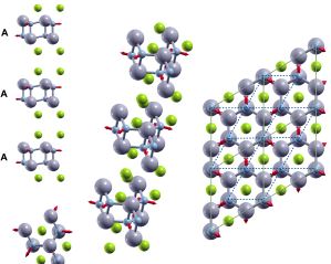
Figure 10: The phonon mode for $\omega_{1}$ at K point shown in a $\sqrt{3}\times\sqrt{3}\times 3$ supercell. The structure is repeated along the $\hat{c}$ axis to show the AAA stacking as compared to the ABC stacking of Fig. 1. Left top: Side view along $\hat{a}-\hat{c}$ plane. Left bottom: Top view along $\hat{a}-\hat{b}$ plane. Middle: Side view tilted to present the displacements. Right: Top view of $2\sqrt{3}\times 2\sqrt{3}$ cell showing the periodicity of the supercell with the solid gray lines, and the dashed blue lines show the $1\times 1$ unit cell.

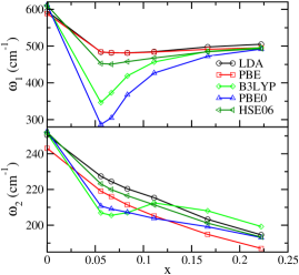
Figure 11: Frequencies as a function of doping for the mode with high electron-phonon coupling with different approximations.

The intervalley phonon $\omega_{1}$ is softened significantly when doped, for all functionals. This softening in the low-doping limit is weaker for the local functionals (LDA/PBE); the change between the undoped and weakly doped modes is $\sim 100$ cm^-1. It becomes substantial as the exact exchange fraction is enhanced, $\sim 300$ cm^-1 for PBE0. Furthermore, the softening decreases as a function of doping. In the case of PBE0 the softening at $x=1/18$ is $40\%$ of the phonon frequency at $2/9$. It is worthwhile to stress that in the HF approximation (not shown here), as the non-magnetic state is unstable towards a magnetic instability, (see Sec. IV.2), the phonon frequencies are imaginary. We explicitly verify this by calculating the phonon frequencies of the undistorted structure.

For the other intervalley phonon, $\omega_{2}$, the mode is also softened when doped, but it decreases as a function of doping. The softening of the frequency when doped is $\sim 30-50$ cm^-1, and smaller than the softening of the $\omega_{1}$. Therefore, the main contribution to the electron-phonon coupling comes from the phonon mode $\omega_{1}$.

In metals, a prominent softening of the phonon frequency is a fingerprint of electron-phonon coupling. Thus the phonon frequency calculations suggest that the intervalley electron-phonon coupling of the mode $\omega_{1}$ is enhanced in the low-doping limit in a way that is proportional to the amount of exact exchange present in the functional, at least for what concerns non-range-separated functionals. The inclusion of range separation slightly decreases the phonon softening, that, however, remains substantial in the low-doping limit.

IV.5 Electron-Phonon Coupling of Intervalley Phonons

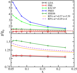
Figure 12: Electron-phonon coupling matrix elements ratio of the doped to the undoped system, $g/g_{0}$, obtained with different approximations, shown in comparison with the $\chi_{s}/\chi_{0s}$ results obtained with the RPA calculations. The panel below is a detailed view of the panel above.

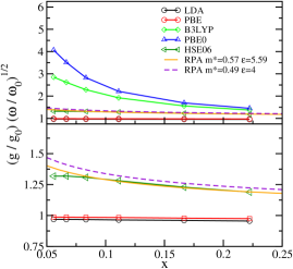
Figure 13: Electron-phonon coupling matrix elements ratio of the doped to the undoped system, scaled with the frequencies $\frac{g}{g_{0}}\sqrt{\frac{\omega}{\omega_{0}}}$, obtained with different approximations, shown in comparison with the $\chi_{s}/\chi_{0s}$ results obtained with the RPA calculations. The panel below is a detailed view of the panel above.

The electron-phonon coupling matrix elements for a mode $\nu$ at a phonon momentum $\mathbf{q}={\bf K}$ for electronic states at the bottom of each valley, namely ${\bf k}={\bf K}$, are defined as

$$g^{\nu}_{\mathbf{K},\mathbf{2K}}=\sum_{A\alpha}\frac{e^{A\alpha}_{\mathbf{K}\nu}}{\sqrt{2M_{A}\omega_{\mathbf{K}\nu}}}\langle\mathbf{K}|\frac{\delta v_{SCF}}{\delta u^{\mathbf{K}}_{A\alpha}}|\mathbf{2K}\rangle,$$ (3)

where $A$ labels the atoms in the unit cell, $\alpha$ is the Cartesian coordinate, and $u^{\mathbf{K}}_{A\alpha}$ is the Fourier transform of the phonon displacement of atom $A$ along direction $\alpha$, with phonon frequency, $\omega_{\mathbf{K}\nu}$, and $v_{SCF}$ is the periodic part of the screened potential.

The matrix element defined in Eq. (3) can be calculated in a frozen phonon approach. We consider a $\sqrt{3}\times\sqrt{3}\times 1$ supercell. As both the special points ${\bf K}$ and ${\bf 2K}$ fold at ${\bf\Gamma}$ when considering the supercell Brillouin zone, the electron-phonon matrix element in the supercell is

$${\tilde{g}}^{\nu}_{\mathbf{\Gamma}n,\mathbf{\Gamma}m}=\langle\mathbf{\Gamma}n|\Delta V|\mathbf{\Gamma}m\rangle$$ (4)

where $m,n$ are band indexes running from $1$ to $2$. Indeed as the valleys at ${\bf K}$ and ${\bf 2K}$ in the Brillouin zone of the unit cell now fold at ${\bf\Gamma}$ of the supercell, there are two degenerate bands, each one twofold degenerate due to spin. The operator $\Delta V$ is defined as

$$\Delta V=\sum_{A\alpha}\frac{{\tilde{e}}^{A\alpha}_{\mathbf{\Gamma}\nu}}{\sqrt{2M_{A}\omega_{\mathbf{{\bf\Gamma}}\nu}}}\frac{\delta v_{scf}}{\delta u^{\mathbf{\Gamma}}_{A\alpha}}$$ (5)

where now the Cartesian components of the phonon eigenvector ${\tilde{e}}^{A\alpha}_{\mathbf{{\bf\Gamma}}\nu}$ are normalized in the $\sqrt{3}\times\sqrt{3}\times 1$ supercell and can be chosen as real.

Equation 4 can also be obtained in perturbation theory by considering the Hamiltonian of the undistorted supercell $H_{0}$ and $\Delta V$ as perturbation, namely,

$$H=H_{0}+\eta\Delta V$$ (6)

where $\eta$ is an arbitrary small constant that sets the magnitudes of the perturbation or, equivalently, of the phonon displacement.

The calculation of the electron-phonon matrix element in the supercell amounts to calculating in first-order perturbation theory for degenerate states the quantity $\langle n|\Delta V|m\rangle$. The calculation can be simplified even more by noting that the states $|\mathbf{\Gamma}m\rangle$ must be a linear combination of the states $|\mathbf{K}\rangle$ and $|\mathbf{K^{\prime}}\rangle$ in the Brillouin zone of the unit cell. As one can choose freely the states $|\mathbf{\Gamma}m\rangle$ in the degenerate subspace, we make the choice $|\mathbf{\Gamma}1\rangle=|\mathbf{K}\rangle$ and $|\mathbf{\Gamma}2\rangle=|\mathbf{2K}\rangle$. This choice assures that

$$\langle\mathbf{\Gamma}n|\Delta V|\mathbf{\Gamma}n\rangle=0$$ (7)

as this matrix element couples electronic states at the same momentum in the Brillouin zone of the unit cell, via a perturbation with a non-zero modulation.

So we are left with only the off-diagonal matrix elements. By diagonalizing the matrix of the perturbation, we obtain that the effect of the distortion on the electronic structure at linear order is to split the two degenerate valleys at ${\bf\Gamma}$ (see Fig. 8 (c) ) of an amount $\Delta\epsilon=2\eta|\langle\mathbf{\Gamma}1|\Delta V|\mathbf{\Gamma}2\rangle|=2\eta|{\tilde{g}}^{\nu}_{\mathbf{\Gamma}1,\mathbf{\Gamma}2}|$. Therefore we have the electron-phonon coupling in the supercell, $|{\tilde{g}}^{\nu}_{\mathbf{\Gamma}1,\mathbf{\Gamma}2}|=\frac{1}{2}\frac{d\Delta\epsilon}{d\eta}$, that can be obtained by displacing the atoms in a way consistent with the phonon displacement of the intervalley phonon and by performing the derivative of the valley splitting as a function of the distortion.

In order to relate the electron-phonon coupling of the supercell to the one of the unit cell, we have to consider that the modes ${\tilde{e}}^{A\alpha}_{\mathbf{\Gamma}\nu}$ are normalized in the supercell, so that:

$$|g^{\nu}_{\mathbf{K},\mathbf{2K}}|^{2}=3|{\tilde{g}}^{\nu}_{\mathbf{\Gamma}1,\mathbf{\Gamma}2}|^{2}$$ (8)

For simplicity, in the rest of the discussion, we will denote $g=|g^{\nu}_{{\bf K},{\bf 2K}}|$. To calculate the non-interacting electron-phonon coupling, $g_{0}$, as in the case of the susceptibility, we use the insulating parent compound. We then obtain the electron-phonon matrix elements by displacing the atoms along ${\tilde{e}}^{A\alpha}_{\mathbf{\Gamma}\nu}$ obtained from a linear response run using the PBE functional and then by calculating the valley splitting in the supercell. As the relative magnitude of the different Cartesian components in the phonon eigenvector are determined only by the symmetry of the modes, the PBE eigenvector can then be used for all the functionals, without introducing any error.

Table 2: For each doping, and the functional, the fundamental band gap E_g between valence maximum at the $\Gamma$ point and conduction minimum at the K point, effective mass, $m^{*}$, density of states at the Fermi level, $N(0)$, magnetic susceptibility, $\chi_{s}$, and the enhancement factor, $\chi_{s}/\chi_{0s}$, of the magnetic susceptibility, electron-phonon coupling matrix element, $g$, for the phonon mode $\omega_{1}$ at the $\mathbf{K}$ point, with $g_{0}$ calculated from the undoped $x=0$ case, and the enhancement factor, $g/g_{0}$, of the electron-phonon coupling matrix element.

$x$	XC	Eg (eV)	$m^{*}$ (me)	N(0) (states/eV)	$\chi_{s}$ ($\mu_{\rm B}^{2}$/eV)	$\chi_{s}/\chi_{0s}$	$g$ (eV)	$g/g_{0}$
0	Expt.	2.5 Ref.[Yokoya et al., 2004]
0	LDA	1.789	0.577				0.242	1.000
1/18	LDA	1.790	0.551	0.535	$0.588$	$1.099$	0.260	1.074
1/15	LDA	1.788	0.548	0.544	$0.588$	$1.081$	0.260	1.074
1/12	LDA	1.785	0.542	0.552	$0.588$	$1.065$	0.260	1.074
1/9	LDA	1.779	0.531	0.564	$0.588$	$1.043$	0.259	1.070
1/6	LDA	1.764	0.517	0.598	$0.623$	$1.042$	0.254	1.050
2/9	LDA	1.763	0.516	0.717	$0.693$	$0.967$	0.251	1.037
0	PBE	1.760	0.548				0.241	1.000
1/18	PBE	1.757	0.525	0.521	$0.603$	$1.157$	0.263	1.091
1/15	PBE	1.754	0.523	0.529	$0.607$	$1.148$	0.263	1.091
1/12	PBE	1.750	0.518	0.539	$0.613$	$1.137$	0.263	1.091
1/9	PBE	1.746	0.507	0.554	$0.613$	$1.107$	0.262	1.087
1/6	PBE	1.732	0.497	0.595	$0.662$	$1.113$	0.259	1.075
2/9	PBE	1.744	0.497	0.728	$0.766$	$1.052$	0.256	1.062
0	B3LYP	3.072	0.487				0.255	1.000
1/18	B3LYP	2.802	0.365	0.473	$1.361$	$2.877$	0.964	3.780
1/15	B3LYP	2.757	0.353	0.480	$1.167$	$2.431$	0.854	3.349
1/12	B3LYP	2.693	0.340	0.489	$0.967$	$1.978$	0.704	2.761
1/9	B3LYP	2.595	0.324	0.504	$0.808$	$1.603$	0.566	2.220
1/6	B3LYP	2.448	0.318	0.545	$0.758$	$1.391$	0.445	1.745
2/9	B3LYP	2.384	0.328	0.633	$0.808$	$1.277$	0.389	1.525
0	PBE0	3.397	0.477				0.266	1.000
1/18	PBE0	3.047	0.334	0.461	$2.450$	$5.315$	1.577	5.929
1/15	PBE0	2.987	0.322	0.467	$1.750$	$3.747$	1.322	4.970
1/12	PBE0	2.899	0.308	0.474	$1.246$	$2.629$	0.968	3.639
1/9	PBE0	2.773	0.293	0.487	$0.942$	$1.934$	0.704	2.647
1/6	PBE0	2.585	0.290	0.520	$0.826$	$1.589$	0.512	1.925
2/9	PBE0	2.493	0.299	0.570	$0.835$	$1.465$	0.430	1.617
0	HSE06	2.718	0.492				0.261	1.000
1/18	HSE06	2.639	0.459	0.472	$0.774$	$1.640$	0.400	1.533
1/15	HSE06	2.621	0.454	0.478	$0.766$	$1.603$	0.401	1.536
1/12	HSE06	2.597	0.448	0.486	$0.750$	$1.543$	0.395	1.513
1/9	HSE06	2.553	0.435	0.498	$0.728$	$1.462$	0.382	1.464
1/6	HSE06	2.479	0.421	0.532	$0.739$	$1.389$	0.360	1.379
2/9	HSE06	2.448	0.418	0.582	$0.817$	$1.404$	0.346	1.326
0	HF	9.190	0.366
1/18	HF	8.068	0.233	0.356	$-0.237$	$-0.666$
1/15	HF	7.871	0.221	0.360	$-0.291$	$-0.808$
1/12	HF	7.584	0.207	0.366	$-0.430$	$-1.175$
1/9	HF	7.134	0.189	0.376	$-0.967$	$-2.572$
1/6	HF	6.373	0.171	0.405	$14.700$	$36.296$
2/9	HF	5.860	0.165	0.441	$1.934$	$4.386$

The results of the calculation are shown in Fig. 12 and Table 2. While the electron-phonon matrix element is essentially constant when using the LDA/PBE functionals, it is substantially enhanced in the low-doping limit by the inclusion of exact exchange. The enhancement in the low doping limit decreases as the amount of exact exchange decreases, namely in going from the PBE0 to B3LYP functional, as shown in the top panel of Fig. 12. In HSE06, the enhancement is intermediate between PBE and B3LYP, due to the introduction of range separation in the Coulomb term. Table 2 summarizes our results with the exact values of the E_g, $N(0)$, $\chi_{s}$, $\chi_{s}/\chi_{0s}$, $g$, and $g/g_{0}$ obtained up to this point.

There is a contribution of the softening in the phonon frequencies to the enhancement of the electron-phonon matrix element, as also evident from Eq. (3). To eliminate this contribution, we also plot, in Fig. 13, the electron-phonon matrix elements $\frac{g}{g_{0}}\sqrt{\frac{\omega}{\omega_{0}}}$, where $\omega$ is the phonon frequency of the doped and $\omega_{0}$ is the phonon frequency of the undoped structure. Once the contribution of the phonon modes is removed, the agreement between the enhancement of the electron-phonon coupling of the HSE06 functional and the RPA calculation of $\chi_{s}/\chi_{0s}$ is improved.

We finally attempt to estimate the error due to the use of a localized basis set on the electron-phonon coupling, by repeating our calculation with the plane-wave basis sets within the Quantum ESPRESSO method using the PBE functional for the lowest doping $x=1/18$. We find that the error in $g$ is $3.137\%$ when using a localized basis set.

The reason for the enhancement of the electron-phonon matrix element has been explained using a model RPA Hamiltonian in Ref. Calandra et al., 2015. As shown in Ref. Calandra et al., 2015 and in Fig. 8, an intervalley phonon displacement can act as a pseudo-magnetic field by changing the occupations of the valley at ${\bf K}$ and ${\bf K^{\prime}}$ without invoking a finite magnetization. In Ref. Calandra et al., 2015 (Supplemental Material) it was shown that as long as the intervalley Coulomb interaction can be neglected, many-body effects enhance the valley susceptibility in the same way as they enhance the spin susceptibility. Furthermore, it was shown that the electron-phonon coupling of an intervalley phonon inducing a valley polarization (pseudomagnetic field) should have an enhancement electron-phonon interaction directly related to the spin/valley susceptibility by the equation

$$\frac{g}{g_{0}}=\frac{\chi_{s}}{\chi_{0s}}$$ (9)

As the spin (and valley) susceptibility are strongly enhanced at low doping by many-body effects, the same behavior should be found in the intervalley electron-phonon matrix element. Interestingly, following the work of Marchi et al. Marchi et al. (2009), in a 2D 2-valley electron gas the spin susceptibility is mostly enhanced by the exchange interaction. The source of divergence of $\chi_{s}/\chi_{0s}$ is the exchange interaction, as the HF approximation is compared with the RPA calculation, while the correlation effects, taken into account with the Monte Carlo simulations in this work, bring this divergence down. Because $r_{s}<1.5$ for Li_xZrNCl, the RPA and Monte Carlo simulations are identical in the regime of our interest. Therefore, the main source of enhancement is the exchange interaction. This result of enhancement due to the exchange interaction agrees with our findings. Indeed, the similar enhancement of the electron-phonon interaction and of the spin susceptibility confirms the validity of Eq. (9).

V Conclusion

In this study, we have analyzed how the exchange and correlation affect the electronic, magnetic, and vibrational properties of Li-doped ZrNCl, a two-dimensional two-valley semiconductor, using different levels of approximations: HF, DFT with standard approximations, LDA and PBE, hybrid functionals with exact exchange B3LYP and PBE0, and finally, a hybrid functional with exact exchange and range separation, HSE06.

By taking advantage of the parabolic conduction band minima, we have calculated the change in the effective mass and band gap. The HF approximation overestimates the band gap with respect to the experiments and underestimates the effective mass, and similarly, the change in these properties as a function of doping is more drastic with the hybrid functionals with exact exchange, PBE0 and B3LYP. On the other hand, standard DFT approximations show almost constant band gap and effective mass with changing doping. The inclusion of the range separation provides a moderate change in these properties, and the HSE06 results lie between the PBE and B3LYP functionals, and the band gap of the HSE06 functional is in good agreement with the experimental value.

The structure is unstable towards a magnetic and charge density state with the HF approximation. Indeed, at low doping, as the magnetization is introduced, the HF approximation predicts the ground state of the system to be magnetic. This presented itself as negative spin susceptibility up to the doping $x=1/6$, at which it diverges. Parallel to this result, the larger the amount of the exact exchange in the hybrid functionals with PBE0 and B3LYP, the larger is the spin susceptibility enhancement towards the low-doping regime. On the other hand, the LDA and PBE approximations do not present any enhancement of the susceptibility. Only HSE06, a hybrid functional with exact exchange and range separation, shows spin susceptibility enhancement similar to the one obtained from the RPA calculations.

Next, the vibrational phonon modes and the electron-phonon coupling are calculated. The phonon frequency of the mode at the K point with high electron-phonon coupling is softened significantly when a small doping is introduced to the system. The frequency then increases as a function of doping, and both the initial softening and the subsequent increase are larger, the larger the exact exchange.

We have calculated the electron-phonon coupling with the frozen phonon approach, by looking at the effect of the phonon displacement on the electronic bands. Analogously to how magnetic field lifts the spin degeneracy and splits the bands, the phonon mode acts as a pseudo-magnetic field and lifts the valley degeneracy, splitting the electronic bands. This is reflected in our results where inter-valley electron-phonon matrix elements show a similar enhancement as compared to the enhancement in the spin susceptibility.

Therefore, we conclude that a phonon mode can act as a pseudomagnetic field and electron-phonon interaction can cause an intervalley polarization. The resulting electron-electron exchange interaction enhances the intervalley polarization, which in turn affects the superconducting temperature enhancement. Furthermore, the differences between the standard density functionals and those with exact exchange and range separation imply that the description of the susceptibility and electron-phonon coupling with a range-separated hybrid functional would also be important in other 2D weakly doped semiconductors, such as transition-metal dichalcogenides and graphene.

Appendix A Calculation of the Effective Mass

Table 3: The fit parameters to the $E(k)$.

$x$	XC	$a_{2}{\rm(eV/Bohr^{-2}})$	$a_{3}{\rm(eV/Bohr^{-3}})$	$a_{4}{\rm(eV/Bohr^{-4}})$
0	LDA	$2.918$	$-1.222$	$0.463$
1/18	LDA	$3.008$	$-1.098$	$0.123$
1/15	LDA	$3.026$	$-1.076$	$0.063$
1/12	LDA	$3.056$	$-1.041$	$-0.061$
1/9	LDA	$3.118$	$-0.984$	$-0.214$
1/6	LDA	$3.251$	$-0.856$	$-0.542$
2/9	LDA	$3.172$	$-0.600$	$-0.766$
0	PBE	$3.071$	$-1.232$	$0.089$
1/18	PBE	$3.155$	$-1.121$	$-0.186$
1/15	PBE	$3.171$	$-1.097$	$-0.234$
1/12	PBE	$3.199$	$-1.059$	$-0.347$
1/9	PBE	$3.263$	$-0.979$	$-0.534$
1/6	PBE	$3.382$	$-0.837$	$-0.823$
2/9	PBE	$3.299$	$-0.577$	$-1.024$
0	B3LYP	$3.453$	$-1.164$	$-0.387$
1/18	B3LYP	$4.548$	$-1.084$	$-2.244$
1/15	B3LYP	$4.695$	$-1.064$	$-2.425$
1/12	B3LYP	$4.877$	$-1.035$	$-2.607$
1/9	B3LYP	$5.102$	$-0.983$	$-2.766$
1/6	B3LYP	$5.281$	$-0.894$	$-2.519$
2/9	B3LYP	$4.993$	$-0.693$	$-2.052$
0	PBE0	$5.398$	$0.486$	$-0.244$
1/18	PBE0	$4.964$	$-1.070$	$-2.812$
1/15	PBE0	$5.153$	$-1.056$	$-3.049$
1/12	PBE0	$5.387$	$-1.044$	$-3.287$
1/9	PBE0	$5.643$	$-1.008$	$-3.346$
1/6	PBE0	$5.787$	$-0.955$	$-2.792$
2/9	PBE0	$5.470$	$-0.779$	$-2.158$
0	HSE06	$3.421$	$-1.196$	$-0.110$
1/18	HSE06	$3.614$	$-1.106$	$-0.449$
1/15	HSE06	$3.648$	$-1.088$	$-0.495$
1/12	HSE06	$3.699$	$-1.058$	$-0.576$
1/9	HSE06	$3.801$	$-0.998$	$-0.781$
1/6	HSE06	$3.979$	$-0.908$	$-0.979$
2/9	HSE06	$3.916$	$-0.658$	$-1.158$
0	HF	$4.601$	$-1.248$	$-0.883$
1/18	HF	$7.106$	$-1.355$	$-2.774$
1/15	HF	$7.497$	$-1.347$	$-3.057$
1/12	HF	$8.026$	$-1.328$	$-3.369$
1/9	HF	$8.734$	$-1.285$	$-3.680$
1/6	HF	$9.819$	$-1.368$	$-4.211$
2/9	HF	$9.949$	$-1.173$	$-4.098$

We have calculated the effective mass by making a fourth-order polynomial fit to the conduction band, along the direction of $\Gamma$ to K to M points of the Brillouin zone, in a region around 0.1 eV above the Fermi level, and calculating the curvature at the band minimum. In Table 3, we present the fit parameters of the function: $E(k)=a_{0}+a_{1}(k-\mathbf{K})+a_{2}(k-\mathbf{K})^{2}+a_{3}(k-\mathbf{K})^{3}+a_{4}(k-\mathbf{K})^{4}$, with energy in units of eV and $k$ in units of $2\pi/a$. As the absolute value of the energy is not known in the DFT framework, we set the zero of the energy to the bottom of the conduction band, making the constant term $a_{0}$ irrelevant. The third- and fourth-order terms are important, because they show how much the Fermi surface is warped with respect to that of the 2D electron gas.

The full expression for the dispersion $E(k)$ can be found in Ref. Brumme et al., 2014. For simplicity, we have assumed that the anisotropy in the effective mass tensor is small.. Hence, we have chosen the path $\Gamma$ to K to M to take into account the conduction band minimum properly. To understand the isotropy in the effective mass, we calculated the effective mass with the same method for $x=1/18$ with the PBE functional along the path $\Gamma$ to K to $\Gamma$ and obtain $m^{*}=0.58$, and M to K to M and obtain $m^{*}=0.50$, as compared to the one obtained along the path of $\Gamma$ to K to M, $m^{*}=0.53$.

Appendix B Changing the Exact Exchange and Range Separation

In addition to the standard forms of the hybrid functionals, to understand the role of the exact exchange percentage and the range separation, we have modified the parameters.

Table 4: The band gap E_g (eV), effective mass, m^∗ (m_e), density of states $N(0)$ (states/eV) , spin susceptibility $\chi_{s}$ ($\mu_{\rm B}^{2}$/eV), and the spin susceptibility enhancement factor, $\chi_{s}/\chi_{0s}$ for the B3LYP functional with exact exchange percentage changed to intermediate steps of $5\%$ and $10\%$, and for the HSE functional with the range separation parameter changed to an intermediate value of $\omega=0.055$ Å^-1 and to $\omega=0.0$, which is the PBE0 limit.

$x$	XC	Eg	m∗	N(0)	$\chi_{s}$	$\chi_{s}/\chi_{0s}$
0	$5\%$	2.079	0.527
1/18	$5\%$	2.023	0.475	0.508	0.674	1.327
1/9	$5\%$	1.969	0.446	0.545	0.639	1.173
1/6	$5\%$	1.926	0.436	0.592	0.674	1.139
2/9	$5\%$	1.917	0.439	0.789	0.774	0.981
0	$10\%$	2.400	0.512
1/18	$10\%$	2.279	0.434	0.495	0.808	1.632
1/9	$10\%$	2.172	0.398	0.530	0.687	1.296
1/6	$10\%$	2.094	0.389	0.574	0.700	1.220
2/9	$10\%$	2.067	0.395	0.726	0.782	1.077
0	$\omega=0.0$	3.396	0.477
1/18	$\omega=0.0$	3.047	0.333	0.460	2.450	5.315
1/9	$\omega=0.0$	2.772	0.293	0.486	0.942	1.938
1/6	$\omega=0.0$	2.582	0.290	0.520	0.826	1.589
2/9	$\omega=0.0$	2.492	0.300	0.569	0.835	1.468
0	$\omega=0.055$	3.022	0.484
1/18	$\omega=0.055$	2.857	0.421	0.466	1.097	2.354
1/9	$\omega=0.055$	2.704	0.387	0.491	0.826	1.682
1/6	$\omega=0.055$	2.580	0.372	0.525	0.790	1.505
2/9	$\omega=0.055$	2.512	0.368	0.575	0.845	1.470

We have changed the exact exchange percentage of the B3LYP functional from the original $20\%$ to the intermediate values of $5\%$ and $10\%$. In addition, if we set the range separation of the HSE functional to $\omega=0$, then the PBE0 functional must be recovered. We have performed the spin susceptibility calculations with this parameter to check this limit of the HSE06 implementation. Furthermore, we have changed the range separation to an intermediate value of $\omega=0.055$ Å^-1, to observe the change in our values as a function of the range separation parameter. These results are presented in Table 4.

We have observed that slowly increasing the amount of exact exchange in the hybrid functional gradually changes the physical properties. If the results of Table 4 are compared to those in Table 2, a gradual increase in the fundamental band gap, decrease in the effective mass, and increase in the susceptibility are observed with increasing exact exchange percentage.

In addition, the HSE functional with the range separation set to $\omega=0$ gives the PBE0 limit correctly, and the band gap, the effective mass, and the susceptibility are essentially the same. Furthermore, changing the range separation of the HSE functional to an intermediate value of $\omega=0.055$ Å^-1, produces band gap, effective mass, and spin susceptibility values in between the original HSE06 and PBE0. The divergence of the spin susceptibility in the low-doping limit with PBE0 decreases with increased range separation. HSE06 functional gives reasonable results, but the perfect agreement with the experiments would only be produced by a functional with adjusted exact exchange and range separation parameters.

Appendix C Spin Susceptibility as Compared to the Experiments

We present the interacting spin susceptibility $\chi_{s}$ as compared to the experiments in Fig. 14. The experimental data are obtained from Ref. Kasahara et al., 2009, with the corrections as explained in the Supplemental Material of Ref. Kasahara et al., 2009 and the Supplemental Material of Ref. Calandra et al., 2015.

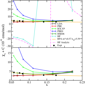
Figure 14: Susceptibility $\chi_{s}$ obtained with different approximations as compared to the experimental data from Refs. Kasahara et al., 2009; Calandra et al., 2015. Panel below is a detailed view of the panel above.

The experimental data of spin susceptibility present the contributions of all the electrons in the system, including the core electrons and orbital contributions of the conducting electrons. These terms are doping independent, and are subtracted from the experimental data to obtain the spin susceptibility of the conduction electrons in the experimental Ref. Kasahara et al., 2009 and the corresponding Supplemental Material: $\chi_{s}=\chi-\chi_{\rm core}^{\rm Li^{+}}-\chi_{\rm core}^{\rm ZrNCl}-\chi_{L}-\chi_{\rm orb}$. The correct form of the Landau diamagnetic susceptibility is given in Ref. Calandra et al., 2015 and the corresponding Supplemental Material as $\chi_{L}=-\chi_{0s}/(3m^{*2})$, and the experimental data presented in Fig. 14 show the corrected result.

Table 5: The Landau diamagnetic susceptibility $\chi_{L}$ in $10^{-6}$emu/mol and the constant $C$ added to the calculated results for each exchange and correlation functional, XC, and HF approximation in both numerical and analytic calculation. RPA values are obtained from Ref. Calandra et al., 2015.

XC	$\chi_{L}$	$C$
LDA	$-8.81$	$-6.81$
PBE	$-9.27$	$-7.27$
B3LYP	$-10.43$	$-8.43$
PBE0	$-10.65$	$-8.65$
HSE06	$-10.32$	$-8.32$
HF	$-13.89$	$-13.89$
RPA	$-8.89$	$-7.77$

For the theoretical results in Fig. 14, we add a constant, $C$, to our calculations to account for the uncertainties in the spin susceptibility contribution of other doping-independent terms. To estimate this constant, we first calculate the Landau susceptibility, $\chi_{L}$, for each approximation, using the effective mass of the undoped structure. A further shift is added to the HSE06 functional to match the experimental enhancement of the susceptibility in the low-doping regime, and the same shift is added to all the other functionals for comparison. Table 5 shows the Landau susceptibility, $\chi_{L}$, and the constant shift, $C$, applied to the calculations in Fig 14.

Appendix D Spin and Valley Magnetic Fields with HSE06 functional

We present how the spin and valley degeneracy is lifted in the case of the HSE06 functional in Fig. 15. As the instabilities do not exist with this functional, we present the electronic bands at the HF energy minimum of each instability for a comparison with the results presented in Fig. 8.

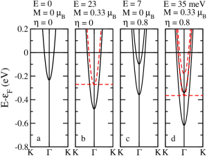
Figure 15: Electronic bands with HSE06 functional with $\sqrt{3}\times\sqrt{3}\times 1$ cell at doping $x=1/18$. (a) Undistorted phase, with the displacement prefactor, $\eta=0$ [see Eq. (6)]; no magnetization $M=0$. (b) Undistorted phase under magnetization. (c) Distorted phase, no magnetization. (d) Distorted phase under magnetization. The difference between the energy of the structure in panel (a) and other structures is given in meV/cell (6 formula units) above each figure. Red dashed lines represent the minority spin and black solid lines represent the majority spin. The Fermi levels of the nonmagnetic case and the majority spin are set to zero and are shown by the black solid horizontal lines. The Fermi level of the minority spin is shown by the red dashed horizontal line.

Figure 15 shows that the introduction of the magnetization and distortion do not lead to an instability with the HSE06 functional, because the energy always increases with respect to the undistorted, nonmagnetic system. Since the system is not at the energy minimum in the case where the total magnetization is fixed, as in Fig. 15 panels (b) and (d), the Fermi energy of the majority and minority spins are not the same, and the zero of the Fermi level of the majority spins is set to zero. All the electrons of the $\sqrt{3}\times\sqrt{3}$ cell are polarized in this case. The bands of the minority spin are not occupied; therefore the Fermi level of the minority spin band is set to the minimum of the conduction band.

Furthermore, we also present the displacement of each atom for the mode $\omega_{1}$ corresponding to $\eta=0.8$ in Table 6. This mode is dominated by the displacements of the N atoms along the $x$-$y$ direction, and therefore is a breathing mode of the N atoms.

Table 6: The displacements of each atom from the undistorted phase corresponding to $\eta=0.8$ for the mode $\omega_{1}$ with large electron-phonon coupling at the K-point. Distances are given in Å.

Atom	$dx$	$dy$	$dz$
Zr	$0.001042$	$-0.000602$	$0.000000$
Zr	$-0.001043$	$-0.000602$	$0.000000$
Zr	$0.000000$	$0.001204$	$0.000000$
Zr	$0.000000$	$-0.001060$	$0.000000$
Zr	$0.000918$	$0.000530$	$0.000000$
Zr	$-0.000918$	$0.000530$	$0.000000$
N	$0.013543$	$-0.007819$	$0.000000$
N	$-0.013543$	$-0.007818$	$0.000000$
N	$-0.000001$	$0.015637$	$0.000000$
N	$0.000000$	$-0.017497$	$-0.000002$
N	$0.015153$	$0.008748$	$-0.000002$
N	$-0.015153$	$0.008749$	$0.000004$
Cl	$0.000000$	$0.000000$	$0.000380$
Cl	$0.000000$	$0.000000$	$-0.000761$
Cl	$0.000000$	$0.000000$	$0.000380$
Cl	$0.000000$	$0.000000$	$-0.000461$
Cl	$0.000000$	$0.000000$	$0.000924$
Cl	$0.000000$	$0.000000$	$-0.000461$

Appendix E Analytic HF Calculation of the Spin Susceptibility Enhancement

The interacting spin susceptibility of multivalley 2D electron gas can be analytically calculated by

$$\frac{\chi_{0s}}{\chi_{s}}=1-\frac{2\alpha r_{s}}{\pi}\int_{0}^{1}dx\frac{xF(x)}{\sqrt{1-x^{2}}}$$ (10)

where $\alpha=\sqrt{g_{v}g_{s}/4}=1$ for a valley $g_{v}=2$ and spin $g_{s}=2$ degeneracy, and $q=2xk_{F}$.

The electron-gas parameter is defined as $r_{s}=1/(a_{B}\sqrt{\pi n})$, where the electron density, $n$ is linked to the doping, $x$, per area, $\Omega$, of 2 formula units of ZrNCl: $n=2x/\Omega$. At the low-doping regime, Li_xZrNCl has $r_{s}<1.5$.

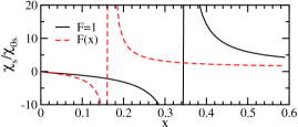
Figure 16: The analytic calculation of the spin susceptibility enhancement with HF approximation, with, $F(x)$, and without, $F=1$, considering the thickness of the 2D electron gas.

For a strictly 2D electron gas, the form factor $F=1$ gives the textbook expression of the spin susceptibility enhancement within the HF approximation Giuliani and Vignale (2005): $\chi_{0s}/\chi_{s}=1-2r_{s}/\pi$.

To take into account the thickness of the 2D electron gas, we obtain an additional term to the form factor. The form factor can be derived by considering the exchange energy $E_{x}=v_{q}F(q)$, with the Coulomb potential, $v_{q}=2\pi/q$. Then we first Fourier-transform the 2D Coulomb interaction with a certain component along the z-direction,

$$FT\left[\frac{1}{r}\right] = \int d^{2}r_{\parallel}\frac{1}{\sqrt{r_{\parallel}^{2}+z^{2}}}e^{-i\vec{q_{\parallel}}\cdot\vec{r_{\parallel}}}$$

$$= \frac{2\pi}{q}e^{-q|z|}$$

and further integrate along the z-direction for an electron gas of a thickness of $a$,

$$\frac{2\pi}{q}F(q) = \frac{2\pi}{q}\frac{1}{a^{2}}\int_{-a/2}^{a/2}dz_{1}\int_{-a/2}^{a/2}dz_{2}e^{-q|z_{1}-z_{2}|}$$

$$= \frac{2\pi}{q}\frac{2}{qa}\left(1+\frac{e^{-qa}-1}{qa}\right)$$

which leads to a form factor of

$$F(q)=\frac{2}{qa^{*}}\left(1+\frac{e^{-qa^{*}}-1}{qa^{*}}\right)$$ (13)

with $q=2xk_{F}$ and the thickness of the 2D electron gas is taken into account in $a^{*}=a/a_{B}$ renormalized by $a_{B}=\epsilon_{M}\hbar^{2}/(m^{*}e^{2})$. The thickness of the electron gas is estimated from the thickness of the ZrN bilayer along the $\hat{c}$ axis and is taken to be $a=2.5$ Å in our calculations. We use the effective mass numerically obtained from the undoped HF structure and the environmental dielectric constant set to $\epsilon_{M}=1$.

In the analytic form of the Hartree-Fock approximation, the metallic screening of the adjacent layers is not taken into account. This is because the electron-electron interaction is not screened in the HF approximation. On the other hand, with the RPA approximation, the electron-electron interaction is screened. In addition, the hopping between the layers is negligible in the present case, hence the HF exchange energy does not contain inter-layer contributions. Indeed the HF exchange energy is equal to: $(-1/2)\int d^{3}rd^{3}r^{\prime}\rho({\bf r},{\bf r}^{\prime})(1/|{\bf r}-{\bf r}^{\prime}|)$, where $\rho({\bf r},{\bf r}^{\prime})$ are the off-diagonal elements of the density matrix. The hopping between layers is negligible, $\rho({\bf r},{\bf r}^{\prime})=0$, if ${\bf r}$ and ${\bf r}^{\prime}$ belong to different layers.

Figure 16 shows the difference between the spin susceptibility enhancement with and without considering the thickness of the 2D electron gas. When the thickness is not taken into account, i.e., $F=1$, the compound is unstable in a larger region of doping, $x<0.34$, while considering the thickness of the 2D electron gas moves the instability region to $x<0.16$, which better agrees with the numerical calculations as shown in Fig. 9. The difference between the instability region with and without considering the thickness of the 2D electron gas, as well as the agreement between the analytic expression and the numerical calculations, gives us confidence in using the form factor $F(x)$.

References

- Saito et al. (2015) Y. Saito, Y. Kasahara, J. Ye, Y. Iwasa, and T. Nojima, Science 350, 409 (2015).
- Lu et al. (2015) J. M. Lu, O. Zheliuk, I. Leermakers, N. F. Q. Yuan, U. Zeitler, K. T. Law, and J. T. Ye, Science 350, 1353 (2015).
- Novoselov et al. (2005) K. S. Novoselov, D. Jiang, F. Schedin, T. J. Booth, V. Khotkevich, S. V. Morozov, and A. K. Geim, Proc. Nat. Acc. Sci. 102, 10451 (2005).
- Xu et al. (2014) X. Xu, W. Yao, D. Xiao, and T.-F. Heinz, Nat. Phys. 10, 343 (2014).
- Zhang et al. (2014) Y. J. Zhang, T. Oka, R. Suzuki, J. T. Ye, and Y. Iwasa, Science 344, 725 (2014).
- Ye et al. (2012) J. T. Ye, Y. J. Zhang, R. Akashi, M. S. Bahramy, R. Arita, and Y. Iwasa, Science 338, 1193 (2012).
- Gregory et al. (1998) D. Gregory, M. Barker, P. Edwards, M. Slaskic, and D. Siddonsa, J. Solid State Chem. 137, 62 (1998).
- Yamanaka et al. (1996) S. Yamanaka, H. Kawaji, K. i. Hotehama, and M. Ohashi, Adv. Mater. 8, 771 (1996).
- Yamanaka et al. (1998) S. Yamanaka, K. Hotehama, and H. Kawaji, Nature (London) 392, 580 (1998).
- Taguchi et al. (2006) Y. Taguchi, A. Kitora, and Y. Iwasa, Phys. Rev. Lett. 97, 107001 (2006).
- Takano et al. (2008a) T. Takano, T. Kishiume, Y. Taguchi, and Y. Iwasa, Phys. Rev. Lett. 100, 247005 (2008a).
- Takano et al. (2008b) T. Takano, A. Kitora, Y. Taguchi, and Y. Iwasa, Journal of Physics and Chemistry of Solids 69, 3089 (2008b).
- Yamanaka et al. (2009) S. Yamanaka, T. Yasunaga, K. Yamaguchi, and M. Tagawa, J. Mater. Chem. 19, 2573 (2009).
- Ye et al. (2010) J. T. Ye, S. Inoue, K. Kobayashi, Y. Kasahara, H. T. Yuan, H. Shimotani, and Y. Iwasa, Nat. Mater. 9, 125 (2010).
- Kasahara et al. (2011) Y. Kasahara, T. Nishijima, T. Sato, Y. Takeuchi, J. Ye, H. Yuan, H. Shimotani, and Y. Iwasa, J. Phys. Soc. Jpn. 80, 023708 (2011).
- Brumme et al. (2014) T. Brumme, M. Calandra, and F. Mauri, Phys. Rev. B 89, 245406 (2014).
- Ekimov et al. (2004) E. A. Ekimov, V. A. Sidorov, E. D. Bauer, N. N. Mel’nik, N. J. Curro, J. D. Thompson, and S. M. Stishov, Nature (London) 428, 542 (2004).
- Heid and Bohnen (2005) R. Heid and K.-P. Bohnen, Phys. Rev. B 72, 134527 (2005).
- Takano et al. (2011) T. Takano, Y. Kasahara, T. Oguchi, I. Hase, Y. Taguchi, and Y. Iwasa, J. Phys. Soc. Jpn. 80, 023702 (2011).
- Botana and Pickett (2014) A. S. Botana and W. E. Pickett, Phys. Rev. B 90, 125145 (2014).
- Calandra et al. (2015) M. Calandra, P. Zoccante, and F. Mauri, Phys. Rev. Lett. 114, 077001 (2015).
- Giuliani and Vignale (2005) G. F. Giuliani and G. Vignale, Quantum Theory of the Electron Liquid (Cambridge, 2005).
- Kasahara et al. (2009) Y. Kasahara, T. Kishiume, T. Takano, K. Kobayashi, E. Matsuoka, H. Onodera, K. Kuroki, Y. Taguchi, and Y. Iwasa, Phys. Rev. Lett. 103, 077004 (2009).
- Taguchi et al. (2010) Y. Taguchi, Y. Kasahara, T. Kishiume, T. Takano, K. Kobayashi, E. Matsuoka, H. Onodera, K. Kuroki, and Y. Iwasa, Physica C: Superconductivity 470, S598 (2010).
- Chen et al. (2001) X. Chen, T. Koiwasaki, and S. Yamanaka, Journal of Solid State Chemistry 159, 80 (2001).
- Shamoto et al. (1998) S. Shamoto, T. Kato, Y. Ono, Y. Miyazaki, K. Ohoyama, M. Ohashi, Y. Yamaguchi, and T. Kajitani, Physica C 306, 7 (1998).
- Kasahara et al. (2010) Y. Kasahara, T. Kishiume, K. Kobayashi, Y. Taguchi, and Y. Iwasa, Phys. Rev. B 82, 054504 (2010).
- Dirac (1930) P. Dirac, Proc. Cambridge Phil. Soc. 26, 376 (1930).
- Perdew and Zunger (1981) J. P. Perdew and A. Zunger, Phys. Rev. B 23, 5048 (1981).
- Perdew et al. (1996) J. P. Perdew, K. Burke, and M. Ernzerhof, Phys. Rev. Lett. 77, 3865 (1996).
- Becke (1993) A. D. Becke, J. Chem. Phys. 98, 5648 (1993).
- Lee et al. (1988) C. Lee, W. Yang, and R. G. Parr, Phys. Rev. B 37, 785 (1988).
- Vosko et al. (1980) S. H. Vosko, L. Wilk, and M. Nusair, Can. J. Phys. 58, 1200 (1980).
- Adamo and Barone (1999) C. Adamo and V. Barone, J. Chem. Phys. 110, 6158 (1999).
- Krukau et al. (2006) A. V. Krukau, O. A. Vydrov, A. F. Izmaylov, and G. E. Scuseria, J. Chem. Phys. 125, 224106 (2006).
- Dovesi et al. (2014a) R. Dovesi, R. Orlando, A. Erba, C. M. Zicovich-Wilson, B. Civalleri, S. Casassa, L. Maschio, M. Ferrabone, M. D. L. Pierre, P. D Arco, Y. Noel, M. Causa, M. Rerat, and B. Kirtman, Int. J. Quantum Chem. 114, 1287 (2014a).
- Weigend and Ahlrichs (2005) F. Weigend and R. Ahlrichs, Phys. Chem. Chem. Phys. 7, 3297 (2005).
- Giannozzi et al. (2009) P. Giannozzi, S. Baroni, N. Bonini, M. Calandra, R. Car, C. Cavazzoni, D. Ceresoli, G. L. Chiarotti, M. Cococcioni, I. Dabo, A. Dal Corso, S. de Gironcoli, S. Fabris, G. Fratesi, R. Gebauer, U. Gerstmann, C. Gougoussis, A. Kokalj, M. Lazzeri, L. Martin-Samos, N. Marzari, F. Mauri, R. Mazzarello, S. Paolini, A. Pasquarello, L. Paulatto, C. Sbraccia, S. Scandolo, G. Sclauzero, A. P. Seitsonen, A. Smogunov, P. Umari, and R. M. Wentzcovitch, J. Phys. Condens. Matter 21, 395502 (2009).
- Dovesi et al. (2014b) R. Dovesi, V. R. Saunders, C. Roetti, R. Orlando, C. M. Zicovich-Wilson, F. Pascale, K. Doll, N. M. Harrison, B. Civalleri, I. J. Bush, Ph. D’Arco, M. Llunell, M. Causà, and Y. Noël, CRYSTAL14 User’s Manual, Università di Torino, Torino (2014b), http://www.crystal.unito.it.
- Ohashi et al. (1989) M. Ohashi, S. Yamanaka, and M. Hattori, Journal of the Ceramic Society of Japan 97, 1181 (1989).
- Yokoya et al. (2004) T. Yokoya, T. Takeuchi, S. Tsuda, T. Kiss, T. Higuchi, S. Shin, K. Iizawa, S. Shamoto, T. Kajitani, and T. Takahashi, Phys. Rev. B 70, 193103 (2004).
- Marchi et al. (2009) M. Marchi, S. De Palo, S. Moroni, and G. Senatore, Phys. Rev. B 80, 035103 (2009).
- Zhang and Das Sarma (2005) Y. Zhang and S. Das Sarma, Phys. Rev. B 72, 075308 (2005).
- Kaur et al. (2010) A. Kaur, E. R. Ylvisaker, Y. Li, G. Galli, and W. E. Pickett, Phys. Rev. B 82, 155125 (2010).
- Adelmann et al. (1999) P. Adelmann, B. Renker, H. Schober, M. Braden, and F. Fernandez-Dias, J. Low Temp. Phys. 117, 449 (1999).
- Cros et al. (2003) A. Cros, A. Cantarero, D. Beltrán-Porter, J. Oró-Solé, and A. Fuertes, Phys. Rev. B 67, 104502 (2003).
- Kitora et al. (2007) A. Kitora, Y. Taguchi, and Y. Iwasa, J. Phys. Soc. Jpn. 76, 023706 (2007).