Validity criteria for Fermi’s golden rule scattering rates applied to metallic nanowires

Abstract

Fermi’s golden rule underpins the investigation of mobile carriers propagating through various solids, being a standard tool to calculate their scattering rates. As such, it provides a perturbative estimate under the implicit assumption that the effect of the interaction Hamiltonian which causes the scattering events is sufficiently small. To check the validity of this assumption, we present a general framework to derive simple validity criteria in order to assess whether the scattering rates can be trusted for the system under consideration, given its statistical properties such as average size, electron density, impurity density et cetera. We derive concrete validity criteria for metallic nanowires with conduction electrons populating a single parabolic band subjected to different elastic scattering mechanisms: impurities, grain boundaries and surface roughness.

I Introduction

Fermi’s golden rule has been applied rather successfully to describe scattering and obtain the transport properties in various condensed matter systems. Ample examples can be found in literature, covering a great variety of devices and applications such as (conventional) metal-oxide-semiconductor transistors Abramo et al. (1994); Mazzoni et al. (1999); Esseni (2004); Jin et al. (2007a); Lizzit et al. (2014), quantum cascade lasers Iotti and Rossi (2001) and nanowire transistors Jin et al. (2007b); Lenzi et al. (2008); Jin et al. (2008), metallic thin films or nanowires Mayadas and Shatzkes (1970); Moors et al. (2014), quasi-1D or -2D materials and devices Pennington and Goldsman (2003); Stauber et al. (2007); Xu and Heinzel (2012); Paussa and Esseni (2013); Dugaev and Katsnelson (2013); Fischetti et al. (2013), as well as for other applications, e.g. the Hall effect Sinitsyn (2008), spin Piéchon and Thiaville (2007) or thermal Shi and Knezevic (2014) transport. Being invoked in a straightforward manner, Fermi’s golden rule, however, comes with some limitations and drawbacks, the most important one being its perturbative nature which essentially restricts the treatment of all scattering events to the level of second-order perturbation theory with respect to the scattering potential $V$.

In order to check whether the perturbative estimate prescribed by Fermi’s golden rule is accurate, the natural thing to do is calculate the higher-order contributions, compare them to the second-order scattering rate and verify whether they are indeed negligible. However, a systematic verification of Fermi’s golden rule up to all orders of the scattering potential is hardly possible for a general scattering potential representing various scattering agents in a condensed matter system, such as impurities, phonons, Coulomb interaction et cetera. Therefore, in most practical cases a higher-order analysis can only be carried out qualitatively or is even missing entirely.

To perform a quantitative analysis of the Fermi’s golden rule scattering rates, we present a framework to obtain the higher-order contributions systematically, leading to validity criteria that can be easily applied. As these criteria are aimed to be as general as possible, we introduce an averaging procedure to capture the essential statistical properties of the scattering potential profiles. Imposing these validity criteria one can check the validity of transport properties obtained through Fermi’s golden rule scattering rates, without the necessity of comparing to non-perturbative treatments of scattering potentials Tešanović et al. (1986); Ness (2006); Martinez et al. (2009); Oh et al. (2012); Rideau et al. (2012); Arenas et al. (2015). A non-perturbative treatment could be too computationally intensive or rely heavily on other approximations, such that it would be difficult to pinpoint which of the different approaches is incorrect and for which reason.

In section II the derivation of Fermi’s golden rule and the higher-order contributions is briefly discussed, as well as the ensemble averaging procedure for the scattering potentials. Concrete examples of validity criteria are derived in section III based on the third- and fourth-order contributions to Fermi’s golden rule for three types of elastic scattering in metallic nanowires assuming a single parabolic band for the conduction electrons. In particular, scattering events due to a single impurity, grain boundaries and surface roughness are considered. Finally, a discussion of the results and a conclusion are respectively presented in section IV and V.

II Fermi’s golden rule

We derive Fermi’s golden rule by making use of the interaction picture in which the evolution operator $U(t)$ satisfies the dynamical equation

$$\mathrm{i}\hbar\frac{\textnormal{d}U\left(t,t_{0}\right)}{\textnormal{d}t}=V(t)U\left(t,t_{0}\right),$$ (1)

with $V$ the scattering potential. This equation can be formally integrated to obtain $U(t,t_{0})$ for all times starting from $t_{0}$. Up to second order in $V$, the overlap between an initial state $\mid\!i\rangle$, having evolved to time $t$, and a final state $\mid\!f\rangle$ (different from the initial state) is given by

$$C_{fi}(t) \equiv\langle f\mid U\left(t,t_{0}\right)\mid i\rangle.$$ (2)

We now proceed with the standard adiabatic approach, considering the limit $t_{0}\rightarrow-\infty$ and assuming a slow turn-on of the potential: $V\rightarrow Ve^{\eta t}$. Playing the role of an inverse time scale, $\eta$ is tuned to be in the regime $t\ll\eta^{-1}\ll t-t_{0}$, from which the overlap integral can be obtained to any order in $V$,

$$C_{fi}(t)$$ (3)

$$\;=\frac{e^{[\eta-\mathrm{i}(E_{i}-E_{f})/\hbar]t}}{E_{i}-E_{f}+\mathrm{i}\hbar\eta}\left(\langle f\mid V\mid i\rangle+\sum_{\alpha}\mkern-3.0mu\int\mkern-5.0mu\textnormal{d}E\;\frac{\textnormal{d}n_{\alpha}}{\textnormal{d}E}\frac{\langle f\mid V\mid E,\alpha\rangle\langle E,\alpha\mid V\mid i\rangle}{E_{i}-E+\mathrm{i}\hbar\eta}+\ldots\right).$$

The intermediate states can be labeled by an energy eigenvalue $E$ and a (sub)band index $\alpha$ to lift the remaining degeneracy. The density of states for each (sub)band is denoted by $\textnormal{d}n_{\alpha}/\textnormal{d}E$. Eq. 3 can be used to obtain the scattering rate $1/\tau_{i\rightarrow f}$ which describes the transition $\mid\!i\rangle\to\;\mid\!f\rangle$, by taking the time derivative of the absolute value squared of the overlap between the two states. In the special case of a one-dimensional conductor of length $L_{z}$, for which the entire phase space is captured by a one-dimensional wave vector $k$ along the transport direction $z$, we get

$$\frac{1}{\tau_{i\rightarrow f}} \equiv\frac{\textnormal{d}}{\textnormal{d}t}\left|C_{fi}(t)\right|^{2}$$ (4)

$$\approx\frac{2\pi}{\hbar}\delta\left(E_{i}-E_{f}\right)\left|\langle f\mid V\mid i\rangle+\sum_{\alpha}\frac{L_{z}}{2\pi}\mkern-2.0mu\int\mkern-4.0mu\textnormal{d}k\;\frac{\langle f\mid V\mid k,\alpha\rangle\langle k,\alpha\mid V\mid i\rangle}{E_{i}-E_{\alpha}(k)+\mathrm{i}\hbar\eta}\right|^{2},$$

where the energy-wave vector relation $E_{\alpha}(k)$ has been introduced. The resulting scattering rate can be interpreted as the total rate incorporating both a direct transition from initial to final state and indirect transitions with one or more intermediate states. Next, we evaluate the integral in Eq. 4 as a contour integral, the integrand having poles $k_{\alpha}$ that satisfy

$$E_{i}-E_{\alpha}(k_{\alpha})+\mathrm{i}\hbar\eta=0.$$ (5)

As the behavior of the $k$-dependent matrix elements determines how the complex contour is to be closed, we proceed by writing out explicitly the matrix elements,

$$\langle f\mid V\mid k,\alpha\rangle\langle k,\alpha\mid V\mid i\rangle$$ (6)

$$\;=\mkern-3.0mu\int\mkern-5.0mu\textnormal{d}^{2}R\;\psi_{f}^{*}(\mathbf{R})\psi_{\alpha}(\mathbf{R})\mkern-3.0mu\int\mkern-5.0mu\textnormal{d}^{2}R^{\prime}\;\psi_{\alpha}^{*}(\mathbf{R}^{\prime})\psi_{i}(\mathbf{R}^{\prime})\mkern-11.0mu\int\limits_{-L_{z}/2}^{+L_{z}/2}\mkern-13.0mu\textnormal{d}z\;V(\mathbf{R},z)\mkern-11.0mu\int\limits_{-L_{z}/2}^{+L_{z}/2}\mkern-13.0mu\textnormal{d}z^{\prime}\;V(\mathbf{R}^{\prime},z^{\prime})\;\frac{e^{-\mathrm{i}(k_{f}-k)z-\mathrm{i}(k-k_{i})z^{\prime}}}{L_{z}^{2}},$$

where the wave functions of the initial and final states as well as of the intermediate states factorize into plane waves along the transport direction $z$ and envelope functions $\psi(\mathbf{R})$ for the transverse directions $\mathbf{R}\equiv(x,y)$. The half plane for which the matrix element product rapidly tends to zero when $k$ is on a semi-circle with increasing radius, is determined by the sign of $z^{\prime}-z$, as long as the $z,z^{\prime}$-dependence of $V$ is such that it does not prevent the exponential decrease due to the plane wave solution. The integration over $k$ gives

$$\mkern-3.0mu\frac{L_{z}}{2\pi}\int\limits_{-\infty}^{+\infty}\mkern-7.0mu\textnormal{d}k\;\frac{e^{-\mathrm{i}(k_{f}-k)z-\mathrm{i}(k-k_{i})z^{\prime}}}{E_{i}-E_{\alpha}(k)+\mathrm{i}\hbar\eta}$$ (7)

$$\;=\mathrm{i}L_{z}\;\sum_{k_{\alpha}}\lim\limits_{k\rightarrow k_{\alpha}}\frac{e^{-\mathrm{i}(k_{f}-k)z-\mathrm{i}(k-k_{i})z^{\prime}}}{E_{i}-E_{\alpha}(k)+\mathrm{i}\hbar\eta}\times\left\{\begin{matrix}\left(k-k_{\alpha}\right)\qquad\textnormal{if}\quad\mathcal{I}\left(k_{\alpha}\right)>0\quad\textnormal{and}\quad z^{\prime}-z<0\\ \left(k_{\alpha}-k\right)\qquad\textnormal{if}\quad\mathcal{I}\left(k_{\alpha}\right)<0\quad\textnormal{and}\quad z^{\prime}-z>0\end{matrix}\right..$$

If the conditions inside the parentheses are not met, the contribution from the pole is zero. This procedure can be repeated for all higher-order contributions, leading to simple diagrammatic rules, as summarized in appendix A. The derivation can also be done more formally to any order in $V$ by using the T-matrix Zubarev et al. (1996).

Figure 1: The poles $k_{\alpha}$ that are picked up by the contour integration as performed in Eq. 7 are shown for an energy-momentum relation symmetric around $k=0$ (e.g. the effective mass model discussed in section III. The imaginary part is negative/positive for negative/positive $k_{\alpha}$ and proportional to the slow turn-on $\eta$.

II.1 Ensemble averaging

In many cases of interest, straightforward application of Fermi’s golden rule suffers from an incomplete knowledge of the scattering potential. In practice, this is reflected in the lack of detailed information regarding the spatial or orientational distribution of the scattering sources in realistic, non-ideal condensed matter systems. The brute force solution to this problem would amount to repeating all relevant simulations for a huge number of potential profiles, while applying statistics to the outcome. However, as such a procedure would lead to unreasonably high computation times when it comes to derive general, but simple validity criteria for Fermi’s golden rule, it becomes paramount to construct a tractable, analytical expression for a generic scattering rate that is averaged over an ensemble of potentials, all representing a particular configuration of the relevant scattering sources. Similar averaging techniques have been applied before to various scattering models, e.g. the random phase approximation for impurities, Gaussian or exponential statistics for Ando’s surface roughness model Ando et al. (1982) and a Gaussian distribution of grain boundaries in the Mayadas-Shatzkes model Mayadas and Shatzkes (1970), but here we present the averaging procedure in a formal way in view to the envisaged validity criteria. In this light, we need to deal with ensemble averages of matrix elements and products thereof involving initial an final states $\mid\!i\rangle,\,\mid\!f\rangle$ as well as intermediate states $\mid\!k,\alpha\rangle$. We introduce the following notation to represent matrix elements explicitly as functionals of the potential profile $V(\mathbf{r})$,

$$\langle i\mid V\mid f\rangle\equiv\mathcal{M}_{if}[V],\qquad\langle i\mid V\mid k,\alpha\rangle\langle k,\alpha\mid V\mid f\rangle\equiv\mathcal{M}_{i\alpha f}[V],\qquad\ldots,$$ (8)

Taking the ensemble average of a matrix element is then accomplished by the following functional integration,

$$\left<\langle i\mid V\mid f\rangle\right>_{V}\equiv\int\mkern-2.0mu\delta V(\mathbf{r})\;g[V(\mathbf{r})]\;\mathcal{M}_{if}\left[V(\mathbf{r})\right],$$ (9)

where $g[V(\mathbf{r})]$, the distribution functional describing the ensemble of relevant potentials, is properly normalized according to

$$\int\mkern-2.0mu\delta V(\mathbf{r})\;g[V(\mathbf{r})]=1.$$ (10)

Generally depending on the type of potentials we need to consider (see sections III.1, III.2 and III.3), $g[V(\mathbf{r})]$ will often be replaced by an ordinary distribution function.

As an example, we quote the averaged scattering rate $1/\tau_{i\rightarrow f}$ up to lowest order in $V$ with the notation introduced in this section,

$$\left\langle\frac{1}{\tau_{i\rightarrow f}}\right\rangle_{V} =\frac{2\pi}{\hbar}\delta\left(E_{i}-E_{f}\right)\left\langle\left|\mathcal{M}_{if}\right|^{2}\right\rangle_{V},$$ (11)

$$\left\langle\left|\mathcal{M}_{if}\right|^{2}\right\rangle_{V} =\int\mkern-2.0mu\delta V(\mathbf{r})\;g[V(\mathbf{r})]\;\left|\mathcal{M}_{if}\left[V(\mathbf{r})\right]\right|^{2}.$$ (12)

III Metallic nanowire

We will develop validity criteria for application of Fermi’s golden rule to scattering rates of electrons in a single parabolic band in a metallic nanowire. The single-electron eigenstates are denoted by $\mid\!k,\mathbf{n}\rangle$ where $\mathbf{n}$ is a shorthand notation indicating the subband indices $(n_{x},n_{y})$ that label the electron subbands along the two transverse directions ($x$ and $y$) and $k$ is the wave vector along the transport direction $z$. Dealing with metallic wires and assuming that the Fermi energy (relative to the bottom of the conduction band) is large compared to $k_{\mathrm{B}}T$ (typically a safe assumption), we may assert that only states with energies equal to the Fermi energy $E_{\mathrm{F}}$ participate in elastic scattering processes. Adopting further the effective mass approximation, we infer parabolic dispersion relations for the conduction band and its subbands, as well as linear group velocities,

$$E_{\alpha}(k)=E_{\alpha}^{0}+B_{\alpha}k^{2},\qquad\left.\frac{\textnormal{d}E_{\alpha}}{\textnormal{d}k}\right|_{E=E_{\mathrm{F}}}\mkern-10.0mu=\theta\left[B_{\alpha}\left(E_{\mathrm{F}}-E_{\alpha}^{0}\right)\right]2\sqrt{B_{\alpha}(E_{\mathrm{F}}-E_{\alpha}^{0})}.$$ (13)

Inserting the dispersion relation into Eq. 7, we obtain

$$\frac{L_{z}}{2\pi} \int\limits_{-\infty}^{+\infty}\mkern-7.0mu\textnormal{d}k\;\frac{\langle f\mid V\mid k,\alpha\rangle\langle k,\alpha\mid V\mid i\rangle}{E_{i}-E_{\alpha}(k)+\mathrm{i}\hbar\eta}=\frac{-\mathrm{i}L_{z}}{2B_{\alpha}k_{\alpha}^{+}}\overline{\mathcal{M}_{f\alpha}\mathcal{M}_{\alpha i}}$$ (14)

$$\;\equiv\, \frac{-\mathrm{i}}{2B_{\alpha}k_{\alpha}^{+}L_{z}}\mkern-3.0mu\int\mkern-5.0mu\textnormal{d}\mathbf{R}\;\psi_{f}^{*}(\mathbf{R})\psi_{\alpha}(\mathbf{R})\mkern-3.0mu\int\mkern-5.0mu\textnormal{d}\mathbf{R}^{\prime}\;\psi_{\alpha}^{*}(\mathbf{R}^{\prime})\psi_{i}(\mathbf{R}^{\prime})$$

$$\times\mkern-12.0mu\int\limits_{-L_{z}/2}^{+L_{z}/2}\mkern-14.0mu\textnormal{d}z\;V(\mathbf{R},z)\mkern-12.0mu\int\limits_{-L_{z}/2}^{+L_{z}/2}\mkern-14.0mu\textnormal{d}z^{\prime}\;V(\mathbf{R}^{\prime},z^{\prime})\;\mathrm{e}^{-\mathrm{i}k_{f}z-\mathrm{i}k_{\alpha}^{+}|z^{\prime}-z|-\mathrm{i}k_{i}z^{\prime}},$$

where $\mathbf{R}$ and $\mathbf{R}^{\prime}$ are transverse position vectors and $k_{\alpha}^{+}\equiv\sqrt{\left(E_{\mathrm{F}}-E^{0}_{\alpha}\right)/B_{\alpha}}$ denotes the positive pole of subband $\alpha$. The line above the product of matrix elements $\overline{\mathcal{M}_{f\alpha}\mathcal{M}_{\alpha i}}$ denotes the replacement of the difference of position coordinates of the intermediate state wave functions $z-z^{\prime}$ by its absolute value and the insertion of the pole $k_{\alpha}^{+}$ into the equation. This procedure is performed in order to keep the full integration domain for $z$ and $z^{\prime}$ from $-L_{z}/2$ to $+L_{z}/2$ while only inserting a single pole into the expression, preventing the splitting of the integration domain according to Eq. 7. This replacement and elimination of one of two poles can be performed for each pair of coordinates along the transport direction that belongs to an intermediate state and is presented in the diagrammatic rules in appendix A.

Carrying out a contour integration in accordance with Eq. 7 and performing the ensemble averaging as explained in section II.1, we get the following validity criteria involving the third- and fourth-order contributions arising from the scattering potential $V$,

$$\frac{\left|\left\langle 2\mathcal{R}\left[\sum\limits_{\alpha}\left(\frac{-\mathrm{i}L_{z}}{2B_{\alpha}k_{\alpha}^{+}}\right)\overline{\mathcal{M}_{f\alpha i}}\mathcal{M}_{if}\right]\right\rangle_{V}\right|}{\left\langle\left|\mathcal{M}_{if}\right|^{2}\right\rangle_{V}} \ll 1,$$ (15)

$$\frac{\left|\left\langle\left|\sum\limits_{\alpha}\left(\frac{-\mathrm{i}L_{z}}{2B_{\alpha}k_{\alpha}^{+}}\right)\overline{\mathcal{M}_{f\alpha i}}\right|^{2}+2\mathcal{R}\left[\sum\limits_{\alpha,\alpha^{\prime}}\left(\frac{-\mathrm{i}L_{z}}{2B_{\alpha}k_{\alpha}^{+}}\right)\left(\frac{-\mathrm{i}L_{z}}{2B_{\alpha^{\prime}}k_{\alpha^{\prime}}^{+}}\right)\overline{\mathcal{M}_{f\alpha\alpha^{\prime}i}}\mathcal{M}_{if}\right]\right\rangle_{V}\right|}{\left\langle\left|\mathcal{M}_{if}\right|^{2}\right\rangle_{V}} \ll 1,$$ (16)

with all the matrix elements being evaluated at $k,k^{\prime}=k_{\alpha}^{+},k_{\alpha^{\prime}}^{+}$. From hereof we will refer to the $n$-th order contribution as $\mathcal{O}(V^{n})$, thus implying that Eqs. 15-16 reduce to $|\mathcal{O}(V^{3})/\mathcal{O}(V^{2})|\ll 1$, $|\mathcal{O}(V^{4})/\mathcal{O}(V^{2})|\ll 1$ in short. Although the lowest higher-order criteria are expected to provide a reliable validity assessment for all higher-order corrections, some higher-order contributions might cancel out exactly or be relatively small due to the properties of the scattering potential. This appears to be the case for the third-order contribution related to scattering events treated in sections III.1-III.2, III.3, the fourth-order validity criterion typically giving rise to a much stronger constraint on the scattering potential size.

Below we consider three examples of elastic scattering represented by an appropriate scattering potential for a localized impurity, grain boundaries and surface roughness.

III.1 Single impurity

For the sake of simplicity, we consider a single impurity at a random position $\mathbf{r}^{\mathsf{imp}}$, the impurity potential taking the form of a delta function with strength $S^{\mathsf{imp}}$,

$$V^{\mathsf{imp}}(\mathbf{r})\equiv S^{\mathsf{imp}}\,\delta(\mathbf{r}-\mathbf{r}^{\mathsf{imp}}).$$ (17)

The unperturbed Hamiltonian describing a quasi-free electron (with effective mass $m^{*}$) in an ideal, boxed wire with zero potential inside the wire and infinite potential outside, and its transverse wave functions are given by:

$$H_{0}(\mathbf{r}) \equiv-\frac{\hbar^{2}\nabla^{2}}{2m^{*}}+\begin{cases}0&\textnormal{if}\quad 0\leqslant x,y\leqslant L_{x},L_{y}\\ +\infty&\textnormal{else}\end{cases},$$ (18)

$$\psi_{\alpha}(x,y) =\left(2/\sqrt{L_{x}L_{y}}\right)\sin\left(n_{\alpha\,x}\pi x/L_{x}\right)\sin\left(n_{\alpha\,y}\pi y/L_{y}\right),\quad n_{\alpha\,x},n_{\alpha\,y}=1,2,3,\ldots$$ (19)

Next, assuming a uniform impurity distribution, we may replace the averaging functional integral by

$$\int\mkern-2.0mu\delta V(\mathbf{r})\;g[V(\mathbf{r})]=\frac{1}{L_{x}L_{y}L_{z}}\int\limits_{0}^{L_{x}}\mkern-3.0mu\textnormal{d}x^{\textnormal{imp}}\mkern-3.0mu\int\limits_{0}^{L_{y}}\mkern-3.0mu\textnormal{d}y^{\textnormal{imp}}\mkern-11.0mu\int\limits_{-L_{z}/2}^{+L_{z}/2}\mkern-13.0mu\textnormal{d}z^{\textnormal{imp}},$$ (20)

in order to compute the required averages occurring in the criteria formulated in Eq. 15-16:

$$\mathcal{O}\left(V^{2}\right)=\left(\frac{S^{\mathsf{imp}}}{L_{x}L_{y}L_{z}}\right)^{2}C_{if}^{\textnormal{imp}},\qquad\mathcal{O}\left(V^{3}\right)=0,$$ (21)

$$\mathcal{O}\left(V^{4}\right)=\sum_{\alpha,\alpha^{\prime}}\left(\frac{L_{z}}{2B_{\alpha}k_{\alpha}^{+}}\right)\left(\frac{L_{z}}{2B_{\alpha^{\prime}}k_{\alpha^{\prime}}^{+}}\right)\left(\frac{S^{\mathsf{imp}}}{L_{x}L_{y}L_{z}}\right)^{4}C_{if\alpha\alpha^{\prime}}^{\textnormal{imp}}.$$ (22)

$C_{if}^{\textnormal{imp.}},C_{if\alpha\alpha^{\prime}}^{\textnormal{imp.}}$ are positive constants of the order of one arising from the wave function parts associated with the transverse directions. Ignoring the factors that are of order one, we get the following validity criterion for the fourth-order contribution,

$$\left|\sum_{\alpha}\left(\frac{L_{z}}{2B_{\alpha}k_{\alpha}^{+}}\right)\left(\frac{S^{\textnormal{imp.}}}{L_{x}L_{y}L_{z}}\right)\right|^{2}\ll 1,$$ (23)

while the third order gives no constraint. The validity check boils down to the comparison of two quantities having the dimension of a volume times an energy, the first one being the impurity strength and the second one arising from the subband density of states at the Fermi level. Note that the criterion is independent of the wire length when the impurity size does not scale with the wire length. The form of the initial and final state wave functions as well as the intermediate states only influences the details of ignored factors that are of order one, the effect being minimal because the impurity position is averaged over the whole wire volume, which smears out any possibly larger effect. The validity criterion mentioned in Eq. 23 is evaluated for different nanowire cross sections and impurity strengths, as shown in Fig. 2.

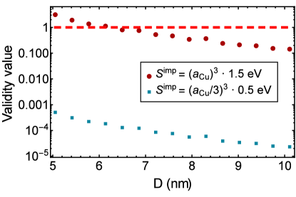
Figure 2: The validity criteria for scattering by a single impurity are evaluated for nanowires with square cross section ($D\equiv L_{x}=L_{y}$) for two impurity strengths: $S^{\mathsf{imp}}=\left(a_{\textnormal{Cu}}\right)^{3}\cdot 1.5$ eV and $S^{\mathsf{imp}}=\left(a_{\textnormal{Cu}}/3\right)^{3}\cdot 0.5$ eV. The evaluation is performed for copper nanowires, assuming a lattice constant $a_{\textnormal{Cu}}\approx 0.361$ nm and an electron density: $n_{\mathsf{e}}\approx 8.47\times 10^{22}$ cm^-3.

III.2 Grain boundaries

Similarly, we may characterize scattering due to grain boundaries by a potential that consists of a sum of Dirac delta functions centered around various axial positions along the wire, representing barrier planes oriented perpendicularly to the transport direction,

$$V^{\mathsf{GB}}(\mathbf{r})\equiv\sum_{j=1}^{N}S^{\mathsf{GB}}\delta\left(z-z_{j}\right),$$ (24)

which, essentially, is borrowed from the grain boundary potential proposed by Mayadas and Shatzkes Mayadas and Shatzkes (1970). Adopting the Mayadas-Shatzkes model, we further assume that all grain boundary planes are uniformly distributed, while neglecting any correlations. The latter are expected to be relevant only if the number of boundary planes is relatively small or if the plane positions were to form a periodic array (thereby enabling the occurrence of resonant tunneling), neither of which is the case for realistic, metallic nanowires. As a consequence, the functional integration may be reduced to an ordinary, multiple integral:

$$\int\mkern-2.0mu\delta V(\mathbf{r})\;g[V(\mathbf{r})]\,(\ldots)=\frac{1}{L_{z}^{N}}\prod_{j=1}^{N}\int\limits_{-L_{z}/2}^{+L_{z}/2}\mkern-15.0mu\textnormal{d}z_{j}\,(\ldots).$$ (25)

We obtain the following contributions for the scattering rates:

$$\mathcal{O}\left(V^{2}\right) \approx N\left(\frac{S^{\mathsf{GB}}}{L_{z}}\right)^{2}\delta_{\mathbf{n}_{i},\mathbf{n}_{f}}\delta_{k_{i},-k_{f}},$$ (26)

$$\mathcal{O}\left(V^{3}\right) \approx-\frac{N!}{(N-2)!}\frac{1}{B_{i}\left|k_{i}\right|^{2}}\left(\frac{S^{\mathsf{GB}}}{L_{z}}\right)^{3}\delta_{\mathbf{n}_{i},\mathbf{n}_{f}}\delta_{k_{i},-k_{f}},$$ (27)

$$\mathcal{O}\left(V^{4}\right) \approx\left[\frac{N!}{(N-4)!}\frac{1}{\left(2B_{i}\left|k_{i}\right|^{2}\right)^{2}}-\frac{N!}{(N-2)!}\frac{1}{\left(2B_{i}\left|k_{i}\right|/L_{z}\right)^{2}}\right]\left(\frac{S^{\mathsf{GB}}}{L_{z}}\right)^{4}\delta_{\mathbf{n}_{i},\mathbf{n}_{f}}\delta_{k_{i},-k_{f}},$$ (28)

with $\delta_{a,b}$ being a Kronecker delta. Considering the limits $1/kL_{z}\ll 1$ and $N\gg 1$, while keeping all contributions of different orders in $kL_{z}/N$, we may formulate the validity criteria related to grain boundary scattering as follows:

$$\left|\frac{\rho^{\mathsf{GB}}S^{\mathsf{GB}}}{B_{i}\left|k_{i}\right|^{2}}\right|\ll 1,\qquad\left|N\left(\frac{\rho^{\mathsf{GB}}S^{\mathsf{GB}}}{2B_{i}\left|k_{i}\right|^{2}}\right)^{2}-N^{2}\left(\frac{S^{\mathsf{GB}}}{2B_{i}\left|k_{i}\right|}\right)^{2}\right|\ll 1,$$ (29)

where $\rho^{\mathsf{GB}}\equiv N/L_{z}$ denotes the grain boundary density. As a result, the second inequality provides the stronger constraint, as can be observed in Fig. 4). Typically, the strongest criteria are found to involve the even powers of $V$, the odd powers appearing in the cross terms and, hence, being reduced stronger under averaging. The criteria for grain boundary scattering also depend on the initial state. The dependence on $k_{i}$ shows that it suffices to check the validity criteria for the lowest appearing $k_{i}$ in a metallic nanowire, giving rise to a maximal ratio in Eq. 29 and providing an upper bound for all $k_{i}$. Note that the second inequality in Eq. 29 is length dependent through its dependence on $N$, even though the lowest-order contribution leads to length independent transport properties when a constant grain boundary density is assumed.

For the single impurity in the previous section, one should bear in mind that the transport properties depend on the wire length, since the effect of a single impurity diminishes with increasing wire length. It seems impossible to make both the transport properties and the validity criteria length independent. For the sake of comparison, a non-perturbative treatment of grain boundary scattering is presented in the following subsection.

III.2.1 Comparison with non-perturbative solution

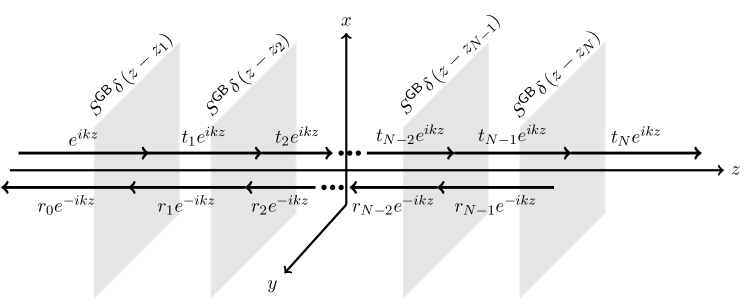
Figure 3: A plane wave with wave vector $k{\mathbf{e}}_{z}$ is injected from the left and propagates through $N$ grain boundary planes at the positions $z_{1}$, $z_{2}$, …, $z_{N}$ with barrier strength $S^{\mathsf{GB}}$. The total transmission probability is given by $|t_{N}|^{2}=1-|r_{0}|^{2}$.

Below, we compare the scattering rates obtained with Fermi’s golden rule with the criteria obtained non-perturbatively by calculating the exact reflection and transmission coefficients, as depicted in Fig. 3. We might expect the non-perturbative solution to diverge from the golden rule solution when the perturbative analysis is to break down according to the validity criterion. Upon invoking the random phase approximation for the positions of the grain boundaries, the transmission coefficient is given by:

$$T=|t_{N}|^{2}=\left|1+\sum_{j=1}^{N}\frac{N!}{(N-j)!j!}\left(-\mathrm{i}\frac{S^{\mathsf{GB}}}{2Bk}\right)^{j}\right|^{-2}.$$ (30)

Up to lowest order, the grain boundary scattering rate obtained by Fermi’s golden rule is proportional to $\left(S^{\mathsf{GB}}\right)^{2}$. If it is to agree with the transmission coefficient given above, one needs to warrant that the contributions to the coefficient that correspond to higher-order terms in $S^{\mathsf{GB}}$, be negligible compared to the second-order contribution, leading to the following constraints:

$$\left|\frac{(N-1)!}{(N-j)!j!}\left(\frac{S^{\mathsf{GB}}}{2Bk}\right)^{j-1}\right|\ll 1\quad\textnormal{for}\;j=2,\ldots,N.$$ (31)

The above constraints agree well with the criteria in Eq. 29 (see Fig. 4) and are also affected by the wire length through the $N$ dependency. Hence, the validity criteria obtained from the higher-order (especially fourth-order) corrections to Fermi’s golden rule are confirmed to provide useful validity constraints. Moreover, they are definitely of interest for cases where non-perturbative treatments, as derived here for grain boundary scattering, are difficult or impossible to perform.

i

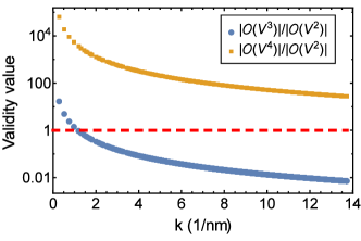
(a)  NW1

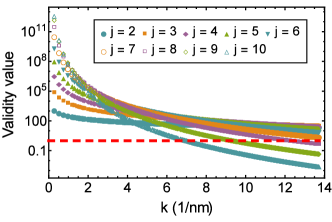
(b)  NW1 (Non-perturbative)

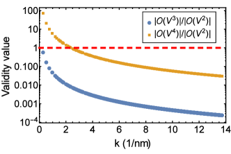
(c)  NW2

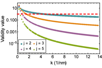
(d)  NW2 (Non-perturbative)

Figure 4: Validity criteria are evaluated for two nanowires with length $L_{z}=100$ nm, width and height $L_{x}=L_{y}\approx 10$ nm, lattice constant $a_{\textnormal{Cu}}\approx 0.361$ nm and electron density of copper: $n_{\mathsf{e}}\approx 8.469\cdot 10^{22}$ cm^-3. The grain boundary parameters are (NW1) $S^{\mathsf{GB}}=a_{\textnormal{Cu}}\cdot 1.5$ eV, $N=10$ (NW2) $S^{\mathsf{GB}}=a_{\textnormal{Cu}}/5\cdot 0.5$ eV, $N=5$.

III.3 Surface roughness

We represent surface roughness by a scattering potential being the difference between the smooth potential well of an ideal wire and potential well profile that is shifted due to the surface roughness. The deviation of the rough surface with respect to the ideal smooth surface is characterized by a surface function $\Delta_{\mathsf{bd}}(x/y,z)$, the subscript “bd” referring to the nanowire boundary surface. We proceed with an analysis for the $x=0$ surface below, for which the potential is given by:

$$V^{\textnormal{\tiny SR}}_{x=0}(\mathbf{r})\equiv H_{0}^{\textrm{pot.}}\left(x-\Delta_{x=0}(y,z),y,z\right)-H_{0}^{\textrm{pot.}}\left(x,y,z\right)\approx U\left[\theta\left(x-\Delta_{x=0}(y,z)\right)-\theta\left(x\right)\right],$$ (32)

where $H_{0}^{\textrm{pot.}}$ is the potential energy part of the Hamiltonian and a finite potential well with barrier height $U$ along the confinement directions is considered, so as to ensure a well-defined shift of the potentials. Because the whole Hamiltonian gets shifted over a distance $\Delta_{x=0}(y,z)$, there also appears a non-zero contribution from near the boundary opposite of the $x=0$ surface. This, however, should not be considered part of the matrix element as it is just an artifact of the notation. Following the same procedure as before, we calculate the matrix elements,

$$\mathcal{M}_{if}^{\textnormal{\tiny SR}(x=0)}\approx\frac{U}{L_{z}}\psi^{*}_{i}(x=0)\psi_{f}(x=0)\mkern-5.0mu\int\limits_{-\infty}^{+\infty}\mkern-7.0mu\textnormal{d}y\;\psi^{*}_{i}(y)\psi_{f}(y)\mkern-11.0mu\int\limits_{-L_{z}/2}^{+L_{z}/2}\mkern-13.0mu\textnormal{d}z\;\Delta_{x=0}(y,z)\mathrm{e}^{-\mathrm{i}(k_{i}-k_{f})z},$$ (33)

The matrix element is expanded linearly in the surface function around $\Delta_{x=0}=0$ to simplify the averaging procedure. The functional integration which, in principle, is still part of the averaging procedure, reduces now to an integration over surface functions (that are considered to be independent) rather than over scattering potential $V$:

$$\int\mkern-5.0mu\delta V(\mathbf{r})\;g\left[V(\mathbf{r})\right]=\mkern-3.0mu\int\mkern-5.0mu\delta\Delta_{x=0}\;g\left[\Delta_{x=0}\right]\cdots\mkern-3.0mu\int\mkern-5.0mu\delta\Delta_{y=L_{y}}\;g\left[\Delta_{y=L_{y}}\right].$$ (34)

In turn, the functional integration over a product of surface roughness functions is assumed to result in a multivariate normal distribution, not specifying the underlying distribution function $g$. The following identities will be used:

$$\left\langle\Delta_{\mathsf{bd}}\right\rangle_{V}=0,\qquad\left\langle\Delta_{\mathsf{bd}_{1}}\Delta_{\mathsf{bd}_{2}}\right\rangle_{V}=\delta_{\textnormal{bd}_{1},\textnormal{bd}_{2}}\Delta^{2}\rho(\mathbf{r}_{1},\mathbf{r}_{2}),\qquad\left\langle\Delta_{\mathsf{bd}_{1}}\Delta_{\mathsf{bd}_{2}}\Delta_{\mathsf{bd}_{3}}\right\rangle_{V}=0,$$ (35)

$$\left\langle\Delta_{\mathsf{bd}_{1}}\Delta_{\mathsf{bd}_{2}}\Delta_{\mathsf{bd}_{3}}\Delta_{\mathsf{bd}_{4}}\right\rangle_{V}=\Delta^{4}\left[\delta_{\textnormal{bd}_{1},\textnormal{bd}_{2}}\delta_{\textnormal{bd}_{3},\textnormal{bd}_{4}}\rho(\mathbf{r}_{1},\mathbf{r}_{2})\rho(\mathbf{r}_{3},\mathbf{r}_{4})+(2\leftrightarrow 3)+(2\leftrightarrow 4)\right].$$

The last line relies on the well-known Wick theorem Wick (1950) (or Isserlis theorem Isserlis (1918)) and establishes various contributions from all possible permutations of the boundary indices. We consider surface roughness functions with mean equal to zero, standard deviation $\Delta$ and a Gaussian autocorrelation function with correlation length $\Lambda$:

$$\rho\left(\mathbf{r}_{1},\mathbf{r}_{2}\right)\equiv\mathrm{e}^{-(\mathbf{r}_{1}-\mathbf{r}_{2})^{2}/(\Lambda^{2}/2)},$$ (36)

which leads to the following results for the second- and third-order contributions:

$$\mathcal{O}\left(V^{2}\right) =\sum_{\textnormal{bd}}\left\langle\left|\mathcal{M}_{if}^{\textnormal{\tiny SR}(\textnormal{bd})}\right|^{2}\right\rangle_{V},\qquad\mathcal{O}\left(V^{3}\right)\approx 0,$$ (37)

$$\left\langle\left|\mathcal{M}_{if}^{\textnormal{\tiny SR}(x=0)}\right|^{2}\right\rangle_{V} \approx\mkern-3.0mu\int\mkern-5.0mu\textnormal{d}z_{1}\mkern-3.0mu\int\mkern-5.0mu\textnormal{d}z_{2}\;\frac{\mathrm{e}^{\mathrm{i}(k_{i}-k_{f})(z_{1}-z_{2})}}{L_{z}^{2}}\rho\left(z_{1},z_{2}\right)\left(V\Delta\right)^{2}\left|\psi_{i}(x=0)\right|^{2}\left|\psi_{f}(x=0)\right|^{2}\;\tensor{*}[_{y_{1}}^{y_{2}}]{C}{{}_{if}^{fi}},$$

where $\tensor{*}[_{y_{1}}^{y_{2}}]{C}{{}_{if}^{fi}}$ is defined by

$$\tensor{*}[_{y_{1}}^{y_{2}}]{C}{{}_{ab}^{cd}} \equiv\mkern-5.0mu\int\limits_{-\infty}^{+\infty}\mkern-7.0mu\textnormal{d}y_{1}\;\psi^{*}_{a}\left(y_{1}\right)\psi_{b}\left(y_{1}\right)\mkern-5.0mu\int\limits_{-\infty}^{+\infty}\mkern-7.0mu\textnormal{d}y_{2}\;\psi^{*}_{c}\left(y_{2}\right)\psi_{d}\left(y_{2}\right)\mathrm{e}^{-(y_{1}-y_{2})^{2}/(\Lambda^{2}/2)},$$ (38)

and analogous short-cuts apply to the integrals over $x$. We develop the two terms containing the fourth-order contributions:

$$\left\langle\left|\sum\limits_{\alpha}\left(\frac{-\mathrm{i}L_{z}}{2B_{\alpha}k_{\alpha}^{+}}\right)\overline{\mathcal{M}_{f\alpha i}^{\textnormal{\tiny SR}}}\right|^{2}+2\mathcal{R}\left[\sum\limits_{\alpha,\alpha^{\prime}}\left(\frac{-\mathrm{i}L_{z}}{2B_{\alpha}k_{\alpha}^{+}}\right)\left(\frac{-\mathrm{i}L_{z}}{2B_{\alpha^{\prime}}k_{\alpha^{\prime}}^{+}}\right)\overline{\mathcal{M}_{f\alpha\alpha^{\prime}i}^{\textnormal{\tiny SR}}}\mathcal{M}_{if}^{\textnormal{\tiny SR}}\right]\right\rangle_{V}$$ (39)

$$\;=\sum_{\alpha,\alpha^{\prime}}\frac{L_{z}}{2B_{\alpha}k_{\alpha}^{+}}\frac{L_{z}}{2B_{\alpha^{\prime}}k_{\alpha^{\prime}}^{+}}\sum_{\textnormal{bd}_{i(1,\ldots,4)}}\mkern-15.0mu\left(\delta_{\textnormal{bd}_{1},\textnormal{bd}_{2}}\delta_{\textnormal{bd}_{3},\textnormal{bd}_{4}}+\textnormal{permutations}\right)$$

$$\;\quad\qquad\qquad\times\left[\left\langle\overline{\mathcal{M}_{f\alpha i}^{\textnormal{\tiny SR}(\textnormal{bd}_{1},\textnormal{bd}_{2})}}\,\overline{\mathcal{M}_{i\alpha^{\prime}f}^{\textnormal{\tiny SR}(\textnormal{bd}_{3},\textnormal{bd}_{4})}}\right\rangle_{V}-2\mathcal{R}\left(\left\langle\overline{\mathcal{M}_{f\alpha\alpha^{\prime}i}^{\textnormal{\tiny SR}(\textnormal{bd}_{1},\textnormal{bd}_{2},\textnormal{bd}_{3})}}\mathcal{M}_{if}^{\textnormal{\tiny SR}(\textnormal{bd}_{4})}\right\rangle_{V}\right)\right],$$

with for example:

$$\left\langle\overline{\mathcal{M}_{f\alpha i}^{\textnormal{\tiny SR}(x=0,x=0)}}\,\overline{\mathcal{M}_{i\alpha^{\prime}f}^{\textnormal{\tiny SR}(x=0,x=0)}}\right\rangle_{V}$$ (40)

$$\;\approx\mkern-3.0mu\int\mkern-5.0mu\textnormal{d}z_{1}\mkern-3.0mu\int\mkern-5.0mu\textnormal{d}z_{2}\mkern-3.0mu\int\mkern-5.0mu\textnormal{d}z_{3}\mkern-3.0mu\int\mkern-5.0mu\textnormal{d}z_{4}\;\frac{\mathrm{e}^{\mathrm{i}k_{f}(z_{4}-z_{1})-\mathrm{i}k_{\alpha}^{+}|z_{1}-z_{2}|+\mathrm{i}k_{i}(z_{2}-z_{3})+\mathrm{i}k_{\alpha^{\prime}}^{+}|z_{3}-z_{4}|}}{L_{z}^{4}}\left[\rho\left(z_{1},z_{2}\right)\rho\left(z_{3},z_{4}\right)+\textnormal{perm.}\right]$$

$$\;\quad\times\left(V\Delta\right)^{4}\left|\psi_{f}\left(x=0\right)\right|^{2}\left|\psi_{\alpha}\left(x=0\right)\right|^{2}\left|\psi_{i}\left(x=0\right)\right|^{2}\left|\psi_{\alpha^{\prime}}\left(x=0\right)\right|^{2}\;\tensor{*}[_{y_{1}}^{y_{2}}]{C}{{}_{f\alpha}^{\alpha i}}\;\tensor{*}[_{y_{3}}^{y_{4}}]{C}{{}_{i\alpha^{\prime}}^{\alpha^{\prime}f}}.$$

We treat the remaining integrals along the transverse and transport directions by approximating the wave functions by the infinite potential well solutions (see appendix B) to obtain the following validity criterion for roughness at the $x=0$ boundary surface, ignoring corrections of order one:

$$\prod_{\alpha=i,f}\textnormal{Val}_{\alpha} \ll 1,$$ (41)

$$\textnormal{Val}_{\alpha} \equiv\sum_{\beta}\sqrt{\frac{\pi}{2}}\frac{\Lambda}{\sqrt{L_{y}L_{z}}}\frac{V\Delta\left|\psi_{\beta}(x=0)\right|^{2}}{\left|2B_{\alpha}k_{\alpha}/L_{z}\right|}\theta^{x}_{\alpha\beta}(\sqrt{8}/\Lambda).$$ (42)

$\theta^{x}_{\alpha\beta}(\sqrt{8}/\Lambda)$ represents a constraint on the difference of wave vectors of Fermi level states $\mid\!\alpha\rangle$ and $\mid\!\beta\rangle$, one of them being the initial or final state and the other an intermediate state. The difference should be less than $\Delta k$, including for the standing wave vector along the transverse direction parallel to the $x=0$ boundary plane:

$$\theta^{x}_{\alpha\beta}(\Delta k) \equiv\begin{cases}1&\textnormal{if}\quad\left|\pi n_{\beta\,y}/L_{y}-\pi n_{\alpha\,y}/L_{y}\right|<\Delta k\textnormal{ and }\left|k_{\beta}-k_{\alpha}\right|<\Delta k\\ 0&\textnormal{else}\end{cases}.$$ (43)

Intermediate states only contribute substantially to the validity criterion when the constraint on the wave vector, as defined in Eq. 43, is met for $\Delta k=\sqrt{8}/\Lambda$ due to the Gaussian surface roughness profile which otherwise exponentially suppresses their contribution, as shown in appendix B. Note that the criterion is again length dependent, although the lowest-order scattering rate results in length independent transport properties. The above criterion is evaluated for two nanowires with different surface roughness properties, the outcome of which is depicted in Fig. 5.

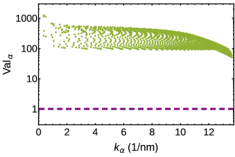
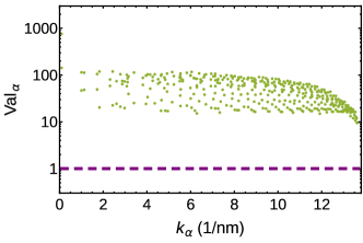
Figure 5: (a) The validity of Fermi’s golden golden rule, used to estimate surface roughness (SR) relaxation times (see Eq. 41) is checked for a Cu nanowire with length $L_{z}=100$ nm, lattice constant $a_{\textnormal{Cu}}\approx 0.361$ nm and electron density $n_{e}\approx 8.469\times 10^{22}$ cm^-3. The wire width and height are taken to be $L_{x}=L_{y}=10$ nm and the SR parameters are chosen to be $\Delta=a_{\textnormal{Cu}}$ and $\Lambda=3a_{\textnormal{Cu}}$. The barrier height is estimated from $V=E_{\textnormal{\tiny F}}+W$, evaluated with bulk values for work function and Fermi energy: $W=4.5$ eV, $E_{\textnormal{\tiny F}}=7$ eV. (b) Same as (a), but with $L_{x}=L_{y}\approx 5$ nm, $\Delta=a_{\textnormal{Cu}}/2$ and $\Lambda=6a_{\textnormal{Cu}}$

IV Discussion

Thorough investigation of the three scattering mechanisms discussed in section III reveals that Fermi’s golden rule may fail to generate reliable scattering rates for realistic scattering potentials, as can be concluded in particular for electrons in metallic nanowires with a single parabolic conduction band from Figs. 2, 4 and 5. The validity can be verified easily in this case by evaluating the validity criteria and depends on the strength of the scattering potential, both in energy and size, and the allowed couplings to intermediate states. The corresponding results clearly indicate that higher-order effects, superseding the second-order perturbation treatment provided by Fermi’s golden rule may come into play and become dominant.

For impurity scattering, the interaction strength, represented by the coefficient that precedes the delta function in the simple model, may be relatively small in practice but the higher-order contributions allow for all Fermi level states as intermediate states, as can be seen in Eq. 23. Hence, the validity of the golden rule scattering rate may be violated for relatively small interaction strengths.

For grain boundaries, the barrier strength associated with a single boundary plane is typically larger than that of a local impurity, but the allowed intermediate states are much more restricted. A perpendicular orientation of grain boundary planes restricts the intermediate states to states with equal subband indices, thus avoiding large summations over $\alpha$ in Eq. 29. However, violation of the scattering rate validity can be reached when the grain boundary strength or density is large enough, which applies most pronouncedly to electron states with low transport momentum. This can be understood physically as these states get trapped most easily in between grain boundaries through higher-order interactions and effectively become bound states, not contributing to the drive current.

Finally, the golden rule scattering rates obtained for surface roughness scattering appear to be most error prone of all three mechanisms. The scattering potential associated with surface roughness is proportional to the energy barrier height outside the metallic wire, which substantially exceeds any internal barriers. Even though the coupling to intermediate states is limited due to the scattering wave vector difference being limited by the inverse of the surface roughness correlation length, the higher-order processes violate the validity criteria for realistic parameters easily. Truly, the validity criteria in Eq. 41 are obtained without rigorously computing the different diagrams and for a linear expansion of the matrix elements for small roughness sizes (which can be improved upon Lizzit et al. (2014); Moors et al. (2015)). However, since the fourth order contribution exceeds the lowest-order scattering rate by many orders of magnitude, the discussion about the application of perturbation theory to surface roughness scattering remains open, not only in relation with metallic nanowires but also in other areas, e.g. when rough edge scattering in graphene ribbons Fischetti and Narayanan (2011) is explored, or when comparison with non-perturbative approaches, based on non-equilibrium Green functions, comes into play Niquet et al. (2014).

V Conclusion

We have developed a framework to derive criteria that can be used to check the validity of Fermi’s golden rule scattering rates systematically, such that their applicability for transport modeling in condensed matter systems can be easily verified. This framework includes an ensemble average over scattering potential profiles, which can be formally represented as a functional integral, leading to general validity criteria that depend on the crucial system parameters, e.g. system size and electron effective mass, and statistical properties of the scattering sources, e.g. impurity strength or surface roughness standard deviation. One can derive a criterion for each higher-order term in the perturbation expansion of the scattering rates.

With the presented framework, we were able to derive simple and general validity criteria for localized impurity scattering (Eq. 23), grain boundary scattering (Eq. 29) and surface roughness scattering (Eq. 41) in metallic nanowires with a single parabolic conduction band, based on the third- and fourth-order corrections to Fermi’s golden rule. The fourth-order correction leads to the strongest validity constraint with which we are able to identify the different aspects having an impact on the validity such as the scattering source strength and its particular coupling properties to intermediate states. All these aspects are uniquely determined for each type of scattering potential and play a crucial role in a rigorous validity analysis of the scattering rates and cannot be taken into account through a merely qualitative analysis of the higher-order corrections, hence confirming the importance and advantages of this type of general criteria. A derivation of validity criteria for nanowires with more general band structures and other (inelastic) scattering mechanisms remains open for future work.

Appendix A Feynman diagrams

Scattering contributions can be evaluated up to arbitrary order with the help of Feynman diagrams. Below, a set of simple diagrammatic rules is summarized together with a proper diagrammatic notation.

• Diagrammatic rules

  • Draw a number of vertices equal to the order of $V$ under consideration.

  • Draw all combinations of directed arrows between two different vertices (no arrow coming back to the same vertex), such that each vertex has a single incoming arrow and a single outgoing arrow, all vertices being connected through a single loop. Two arrows should be labeled $i$ and $f$ so as to represent respectively the initial and final state.

  • If an identical diagram arises from reversing all arrows and renaming all labels but $i$ and $f$, it should be discarded.

• Contributions to the scattering rates

  • All labels unequal to $i$ or $f$ represent electron states at the Fermi level (possibly equal to state $\mid\!i\rangle$ or $\mid\!f\rangle$) and add a factor $L_{z}/2B_{\textnormal{label}}k_{\textnormal{label}}$ to the scattering rate.

  • Add a factor $(-\mathrm{i})^{\textnormal{``number of $V$ between $f$ and $i$'' - 1}}\times(\mathrm{i})^{\textnormal{``number of $V$ between $i$ and $f$'' - 1}}$.

  • For each vertex, add a factor $\langle\textnormal{label incoming arrow}\mid V\mid\textnormal{label outgoing arrow}\rangle$ to the scattering rate.

  • Sum over all Fermi level states for each label not representing the initial or final state and correct the matrix elements by changing the differences in $z$-positions $\Delta z$ that multiply the $k_{\textnormal{label}}$ wave vectors by their absolute value and fixing the sign such that $+\mathrm{i}|k_{\textnormal{label}}||\Delta z|$ appears in the exponential wave function along the $z$-direction if the label appears in between $i$ and $f$ and $-\mathrm{i}|k_{\textnormal{label}}||\Delta z|$ if the label appears in between $f$ and $i$ on the oriented loop running between the vertices.

  • Finally, multiply by $2\pi/\hbar\times\delta(E_{i}-E_{f})$.

All diagrams of the second up to the fourth-order contribution to the scattering rate are shown in Fig. 6. Higher order diagrams can be calculated by applying Wick’s theorem (see Fig. 7 and Fig. 8), which was used to obtain the validity criteria for surface roughness scattering in section III.3.

Figure 6: Feynman diagrams corresponding to the $\mathcal{O}(V^{2})$, $\mathcal{O}(V^{3})$ and $\mathcal{O}(V^{4})$ contributions to the scattering rate.

Figure 7: Diagrammatic representation of the terms that contribute to the validity criteria for surface roughness, as developed in section III.3 (part I).

Figure 8: Diagrammatic representation of the terms that contribute to the validity criteria for surface roughness, as developed in section III.3 (part II).

Appendix B Gaussian integrals

The expression $\tensor{*}[_{y_{1}}^{y_{2}}]{C}{{}_{ab}^{cd}}$ can be evaluated by approximating the wave functions by the infinite potential well solutions (analogously for $\tensor{*}[_{x_{1}}^{x_{2}}]{C}{{}_{ab}^{cd}}$), yielding

$$\tensor{*}[_{y_{1}}^{y_{2}}]{C}{{}_{ab}^{cd}} \approx\sqrt{\frac{\pi}{2}}\frac{\Lambda}{L_{y}}\frac{1}{2}\left\{\mathrm{e}^{-(n_{c}^{y}-n_{d}^{y})^{2}\pi^{2}\Lambda^{2}/8L_{y}^{2}}\left[\delta_{|n_{a}^{y}-n_{b}^{y}|,|n_{c}^{y}-n_{d}^{y}|}\left(1+\delta_{n_{a}^{y},n_{b}^{y}}\right)-\delta_{n_{a}^{y}+n_{b}^{y},|n_{c}^{y}-n_{d}^{y}|}\right]\right.$$ (44)

$$\quad\qquad\qquad\quad\left.+\mathrm{e}^{-(n_{c}^{y}+n_{d}^{y})^{2}\pi^{2}\Lambda^{2}/8L_{y}^{2}}\left(\delta_{n_{a}^{y}+n_{b}^{y},n_{c}^{y}+n_{d}^{y}}-\delta_{|n_{a}^{y}-n_{b}^{y}|,n_{c}^{y}+n_{d}^{y}}i\right)\right\}.$$

Calculation of the remaining integrals along the transport direction yields the second-order contribution as follows:

$$\mkern-13.0mu\int\limits_{-L_{z}/2}^{+L_{z}/2}\mkern-15.0mu\textnormal{d}z_{1}\mkern-10.0mu\int\limits_{-L_{z}/2}^{+L_{z}/2}\mkern-15.0mu\textnormal{d}z_{2}\;\frac{\mathrm{e}^{\mathrm{i}(k_{i}-k_{f})(z_{1}-z_{2})}}{L_{z}^{2}}\rho\left(z_{1},z_{2}\right)\approx\sqrt{\frac{\pi}{2}}\frac{\Lambda}{L_{z}}\mathrm{e}^{-(k_{i}-k_{f})^{2}\Lambda^{2}/8}.$$ (45)

Evaluation of the fourth-order contribution requires a careful treatment of the position differences appearing in the wave functions. We get for example:

$$\int\limits_{-L_{z}/2}^{+L_{z}/2}\mkern-15.0mu\textnormal{d}z_{1}\mkern-10.0mu\int\limits_{-L_{z}/2}^{+L_{z}/2}\mkern-15.0mu\textnormal{d}z_{2}\mkern-10.0mu\int\limits_{-L_{z}/2}^{+L_{z}/2}\mkern-15.0mu\textnormal{d}z_{3}\mkern-10.0mu\int\limits_{-L_{z}/2}^{+L_{z}/2}\mkern-15.0mu\textnormal{d}z_{4}\;\frac{\mathrm{e}^{\mathrm{i}k_{f}(z_{4}-z_{1})-\mathrm{i}k_{\alpha}^{+}|z_{1}-z_{2}|+\mathrm{i}k_{i}(z_{2}-z_{3})+\mathrm{i}k_{\alpha^{\prime}}^{+}|z_{3}-z_{4}|}}{L_{z}^{4}}\rho\left(z_{1},z_{2}\right)\rho\left(z_{3},z_{4}\right)$$ (46)

$$\;\approx\frac{\pi}{2}\left(\frac{\Lambda}{L_{z}}\right)^{2}\frac{2-2\cos\left[\left(k_{f}-k_{i}\right)L_{z}\right]}{\left(k_{f}-k_{i}\right)^{2}L_{z}^{2}}\sum_{\pm,\pm^{\prime}}\frac{\mathrm{e}^{-(k_{i}\pm k_{\alpha}^{+})^{2}\Lambda^{2}/8}}{2}\frac{\mathrm{e}^{-(k_{f}\pm^{\prime}k_{\alpha^{\prime}}^{+})^{2}\Lambda^{2}/8}}{2},$$

$$\int\limits_{-L_{z}/2}^{+L_{z}/2}\mkern-15.0mu\textnormal{d}z_{1}\mkern-10.0mu\int\limits_{-L_{z}/2}^{+L_{z}/2}\mkern-15.0mu\textnormal{d}z_{2}\mkern-10.0mu\int\limits_{-L_{z}/2}^{+L_{z}/2}\mkern-15.0mu\textnormal{d}z_{3}\mkern-10.0mu\int\limits_{-L_{z}/2}^{+L_{z}/2}\mkern-15.0mu\textnormal{d}z_{4}\;\frac{\mathrm{e}^{\mathrm{i}k_{f}(z_{4}-z_{1})-\mathrm{i}k_{\alpha}^{+}|z_{1}-z_{2}|-\mathrm{i}k_{\alpha^{\prime}}^{+}|z_{2}-z_{3}|+\mathrm{i}k_{i}(z_{3}-z_{4})}}{L_{z}^{4}}\rho\left(z_{1},z_{2}\right)\rho\left(z_{3},z_{4}\right)$$ (47)

$$\;\approx\frac{\pi}{2}\left(\frac{\Lambda}{L_{z}}\right)^{2}\mathrm{e}^{-(k_{f}-k_{i})^{2}\Lambda^{2}/8}\sum_{\pm,\pm^{\prime}}\frac{\mathrm{e}^{-(k_{f}\pm k_{\alpha}^{+})^{2}\Lambda^{2}/8}}{2}\frac{\delta_{k_{\alpha^{\prime}}^{+},\pm^{\prime}k_{f}}}{2}.$$

References

- Abramo et al. (1994) A. Abramo, L. Baudry, R. Brunetti, R. Castagne, M. Charef, F. Dessenne, P. Dollfus, R. Dutton, W. Engl, R. Fauquembergue, et al., Electron Devices, IEEE Transactions on 41, 1646 (1994).
- Mazzoni et al. (1999) G. Mazzoni, A. L. Lacaita, L. M. Perron, and A. Pirovano, Electron Devices, IEEE Transactions on 46, 1423 (1999).
- Esseni (2004) D. Esseni, Electron Devices, IEEE Transactions on 51, 394 (2004).
- Jin et al. (2007a) S. Jin, M. V. Fischetti, and T.-W. Tang, Electron Devices, IEEE Transactions on 54, 2191 (2007a).
- Lizzit et al. (2014) D. Lizzit, D. Esseni, P. Palestri, and L. Selmi, Journal of Applied Physics 116, 223702 (2014).
- Iotti and Rossi (2001) R. C. Iotti and F. Rossi, Physical Review Letters 87, 146603 (2001).
- Jin et al. (2007b) S. Jin, M. V. Fischetti, and T.-w. Tang, Journal of Applied Physics 102, 083715 (2007b).
- Lenzi et al. (2008) M. Lenzi, P. Palestri, E. Gnani, S. Reggiani, A. Gnudi, D. Esseni, L. Selmi, and G. Baccarani, Electron Devices, IEEE Transactions on 55, 2086 (2008).
- Jin et al. (2008) S. Jin, T.-W. Tang, and M. V. Fischetti, Electron Devices, IEEE Transactions on 55, 727 (2008).
- Mayadas and Shatzkes (1970) A. F. Mayadas and M. Shatzkes, Physical Review B 1, 1382 (1970).
- Moors et al. (2014) K. Moors, B. Sorée, Z. Tőkei, and W. Magnus, Journal of Applied Physics 116, 063714 (2014).
- Pennington and Goldsman (2003) G. Pennington and N. Goldsman, Physical Review B 68, 045426 (2003).
- Stauber et al. (2007) T. Stauber, N. Peres, and F. Guinea, Physical Review B 76, 205423 (2007).
- Xu and Heinzel (2012) H. Xu and T. Heinzel, Journal of Physics: Condensed Matter 24, 455303 (2012).
- Paussa and Esseni (2013) A. Paussa and D. Esseni, Journal of Applied Physics 113, 093702 (2013).
- Dugaev and Katsnelson (2013) V. Dugaev and M. Katsnelson, Physical Review B 88, 235432 (2013).
- Fischetti et al. (2013) M. V. Fischetti, J. Kim, S. Narayanan, Z.-Y. Ong, C. Sachs, D. K. Ferry, and S. J. Aboud, Journal of Physics: Condensed Matter 25, 473202 (2013).
- Sinitsyn (2008) N. Sinitsyn, Journal of Physics: Condensed Matter 20, 023201 (2008).
- Piéchon and Thiaville (2007) F. Piéchon and A. Thiaville, Physical Review B 75, 174414 (2007).
- Shi and Knezevic (2014) Y. Shi and I. Knezevic, Journal of Applied Physics 116, 123105 (2014).
- Tešanović et al. (1986) Z. Tešanović, M. V. Jarić, and S. Maekawa, Physical review letters 57, 2760 (1986).
- Ness (2006) H. Ness, Journal of Physics: Condensed Matter 18, 6307 (2006).
- Martinez et al. (2009) A. Martinez, A. R. Brown, N. Seoane, and A. Asenov, in Journal of Physics: Conference Series, Vol. 193 (IOP Publishing, 2009) p. 012047.
- Oh et al. (2012) J. H. Oh, M. Shin, and M.-G. Jang, Journal of Applied Physics 111, 044304 (2012).
- Rideau et al. (2012) D. Rideau, Y. Niquet, O. Nier, P. Palestri, D. Esseni, V. Nguyen, F. Triozon, I. Duchemin, D. Garetto, and L. Smith, Mobility in FDSOI devices: Monte Carlo and Kubo Greenwood approaches compared to NEGF simulations (na, 2012).
- Arenas et al. (2015) C. Arenas, R. Henriquez, L. Moraga, E. Muñoz, and R. C. Munoz, Applied Surface Science 329, 184 (2015).
- Zubarev et al. (1996) D. N. Zubarev, V. G. Morozov, and G. Röpke, Statistical mechanics of nonequilibrium processes, Vol. 1 (Akademie Verlag Berlin, 1996).
- Ando et al. (1982) T. Ando, A. B. Fowler, and F. Stern, Reviews of Modern Physics 54, 437 (1982).
- Wick (1950) G.-C. Wick, Physical review 80, 268 (1950).
- Isserlis (1918) L. Isserlis, Biometrika , 134 (1918).
- Moors et al. (2015) K. Moors, B. Sorée, and W. Magnus, Journal of Applied Physics 118, 124307 (2015).
- Fischetti and Narayanan (2011) M. V. Fischetti and S. Narayanan, Journal of Applied Physics 110, 083713 (2011).
- Niquet et al. (2014) Y.-M. Niquet, V.-H. Nguyen, F. Triozon, I. Duchemin, O. Nier, and D. Rideau, Journal of Applied Physics 115, 054512 (2014).