Two value ranges for symmetric self-mappings of the unit disc

Abstract

Let $\mathbb{D}$ be the unit disc and $z_{0}\in\mathbb{D}.$ We determine the value range $\{f(z_{0})\,|\,f\in\mathcal{R}^{\geq}\}$, where $\mathcal{R}^{\geq}$ is the set of holomorphic functions $f:\mathbb{D}\to\mathbb{D}$ with $f(0)=0$ and $f^{\prime}(0)\geq 0$ that have only real coefficients in their power series expansion around $0$, and the smaller set $\{f(z_{0})\,|\,f\in\mathcal{R}^{\geq},\text{$f$ is typically real}\}.$
Furthermore, we describe a third value range $\{f(z_{0})\,|\,f\in\mathcal{I}\}$, where $\mathcal{I}$ consists of all univalent self-mappings of the upper half-plane $\mathbb{H}$ with hydrodynamical normalization which are symmetric with respect to the imaginary axis.

Keywords: value ranges, radial Loewner equation, chordal Loewner equation, univalent functions, typically real functions

2010 Mathematics Subject Classification: 30C55, 30C80.

1 Introduction

There are many results that determine value regions $V_{A}(z_{0})=\{f(z_{0})\,|\,f\in A\}$, where $z_{0}$ is a fixed point and $f$ runs through a set $A$ of analytic functions in the unit disc $\mathbb{D}$ or the upper half-plane $\mathbb{H}$. In this paper we describe $V_{A}(z_{0})$ for the following cases.

In Section 2, we let $A$ be the set of all univalent self-mappings of $\mathbb{H}$ with hydrodynamical normalization which are symmetric with respect to the imaginary axis. The value set $V_{A}(z_{0})$ can be computed by analysing the reachable set of a certain Loewner equation.

In Section 3, we consider the case where $A$ consists of all typically real mappings $f:\mathbb{D}\to\mathbb{D}$ with $f(0)=0$ and $f^{\prime}(0)>0.$ It turns out that $V_{A}(z_{0})$ is equal to the value set $\{f(z_{0})\,|\,f\in A\text{ and $f$ is univalent}\}$, which has been determined by Prokhorov in [Pro92]. A univalent self mapping $f:\mathbb{D}\to\mathbb{D}$ with $f(0)=0$ and $f^{\prime}(0)>0$ is typically real if and only if $f(\overline{z})=\overline{f(z)},$ i.e. $f$ is symmetric with respect to the real axis. We also consider the smaller set $\{f(z_{0})\,|\,f\in A\text{ and $f^{\prime}(0)=\tau$}\}$ for fixed $\tau\in(0,1].$
Furthermore, we determine $V_{A}(z_{0})$ for the case where $A$ consists of all self-mappings $f:\mathbb{D}\to\mathbb{D}$ with $f(0)=0$ and $f^{\prime}(0)\geq 0$ that have only real coefficients in its power series expansion around $0$.

Acknowledgements: The authors would like to thank the anonymous referee for their time and effort taken to review our manuscript, and for their helpful suggestions.

2 Hydrodynamic normalization

Let $\mathcal{H}$ be the set of all univalent, i.e. holomorphic and injective, mappings $f:\mathbb{H}\to\mathbb{H}$ with hydrodynamic normalization at infinity, i.e.

$$f(z)=z-\frac{c}{z}+\gamma(z),$$ (2.1)

where $\operatorname{hcap}(f):=c\geq 0$, which is usually called half-plane capacity, and $\gamma$ satisfies $\angle\lim_{z\to\infty}z\cdot\gamma(z)=0.$

Remark 2.1.

Let $f\in\mathcal{H}$ with $\operatorname{hcap}(f)=c.$ If we transfer $f$ to the unit disc by conjugation by the Cayley transform, then we obtain a function $\tilde{f}:\mathbb{D}\to\mathbb{D}$ having the expansion

$$\tilde{f}(z)=z-\frac{c}{4}(z-1)^{3}+\tilde{\gamma}(z),$$

where $\angle\lim_{z\to 1}\frac{\tilde{\gamma}(z)}{(z-1)^{3}}=0.$

Let $z_{0}\in\mathbb{H}.$ From the boundary Schwarz lemma it is clear that $\text{Im}\,(f(z_{0}))\geq\text{Im}\,(z_{0})$ and $\text{Im}\,(f(z_{0}))=\text{Im}\,(z_{0})$ if and only if $f$ is the identity. It is quite simple to show that

$$V_{\mathcal{H}}(z_{0})=\{w\in\mathbb{H}\,|\,\text{Im}\,(w)>\text{Im}\,(z_{0})\}\cup\{z_{0}\},$$

see [RS14], Theorem 2.4.

Next, let

$$\mathcal{I}=\{f\in\mathcal{H}\,|\,f(-\overline{z})=-\overline{f(z)}\text{ for all $z\in\mathbb{H}$}\}.$$

$\mathcal{I}$ consists of all $f\in\mathcal{H}$ such that the image $f(\mathbb{H})$ is symmetric with respect to the imaginary axis.

Theorem 2.2.

Let $z_{0}\in\mathbb{H}.$ If $\text{Re}\,(z_{0})=0$, then $V_{\mathcal{I}}(z_{0})=\{z_{0}+it\,|\,t\in[0,\infty)\}.$
Next, assume $\text{Re}\,(z_{0})>0$ and define the two curves $C(z_{0})$ and $D(z_{0})$ by

$$C(z_{0})=\left\{\sqrt{z_{0}^{2}-2t}\,|\,t\in[0,\infty)\right\}=\{x+iy\in\mathbb{H}\,|\,x\cdot y=\text{Re}\,(z_{0})\text{Im}\,(z_{0}),\,x\in(0,\text{Re}\,(z_{0})]\},$$

$$D(z_{0})=\left\{z_{0}+e^{i\arg(z_{0})}\cdot t\,|\,t\in[0,\infty)\right\}.$$

Then, the set $\overline{V_{\mathcal{I}}(z_{0})}$ is the closed subset of $\mathbb{H}$ bounded by $C(z_{0})$ and $D(z_{0}),$ and $V_{\mathcal{I}}(z_{0})=\{z_{0}\}\cup\overline{V_{\mathcal{I}}(z_{0})}\setminus D(z_{0}).$
The case $\text{Re}\,(z_{0})<0$ follows from the case $\text{Re}\,(z_{0})>0$ by reflection w.r.t the imaginary axis.

The value set $f^{-1}(z_{0})$ for the inverse functions is given in a quite similar way.

Theorem 2.3.

Let $z_{0}\in\mathbb{H}$ and define

$$V_{\mathcal{I}}^{*}(z_{0})=\{f^{-1}(z_{0})\,|\,f\in\mathcal{I},z_{0}\in f(\mathbb{H})\}.$$

If $\text{Re}\,(z_{0})=0$, then $V_{\mathcal{I}}^{*}(z_{0})=\{z_{0}-it\,|\,t\in[0,\text{Im}\,(z_{0}))\}.$
Next, assume $\text{Re}\,(z_{0})>0$ and define the two curves $C^{*}(z_{0})$ and $D^{*}(z_{0})$ by

$$C^{*}(z_{0})=\left\{\sqrt{z_{0}^{2}+2t}\,|\,t\in[0,\infty)\right\}=\{x+iy\in\mathbb{H}\,|\,x\cdot y=\text{Re}\,(z_{0})\text{Im}\,(z_{0}),\,x\in[\text{Re}\,(z_{0}),\infty)\},$$

$$D^{*}(z_{0})=\left\{z_{0}-e^{i\arg(z_{0})}\cdot t\,|\,t\in[0,|z_{0}|)\right\}.$$

Then, the closure $\overline{V_{\mathcal{I}}^{*}(z_{0})}$ is the closed subset of $\mathbb{H}$ bounded by the curves $C^{*}(z_{0}),$ $D^{*}(z_{0})$ and the positive real axis. The set $V_{\mathcal{I}}^{*}(z_{0})$ is given by $V_{\mathcal{I}}^{*}(z_{0})=\{z_{0}\}\cup\overline{V_{\mathcal{I}}^{*}(z_{0})}\setminus(D^{*}(z_{0})\cup[0,\infty)).$
The case $\text{Re}\,(z_{0})<0$ follows from the case $\text{Re}\,(z_{0})>0$ by reflection w.r.t the imaginary axis.

Figure 1 shows the curves $C(1+i)$ and $D(1+i)$ (dashed), as well as $C^{*}(1+i)$ and $D^{*}(1+i)$.

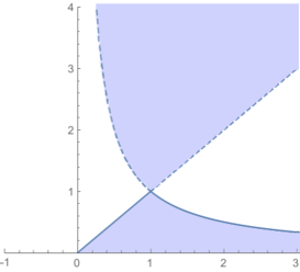
Figure 1: $V_{\mathcal{I}}(1+i)$ and $V_{\mathcal{I}}^{*}(1+i).$

Proof of Theorem 2.2.

Without loss of generality we may assume that $z_{0}\in Q_{1}:=\{z\in\mathbb{C}\,|\,\text{Re}\,z\geq 0,\text{Im}\,z>0\}.$

Now consider the chordal Loewner equation

$$\dot{f}_{t}(z)=\int_{\mathbb{R}}\frac{1}{a-f_{t}(z)}\,\alpha_{t}(da) t\geq 0 f_{0}(z)=z\in\mathbb{H}$$ for a.e. ,  , (2.2)

where $\alpha_{t}$ is a Borel probability measure on $\mathbb{R}$ for every $t\geq 0$, and the function $t\mapsto\int_{\mathbb{R}}\frac{1}{a-z}\,\alpha_{t}(da)$ is measurable for every $z\in\mathbb{H}.$ For every $f\in\mathcal{H}$ there exists $T>0$ and such a family $\{\alpha_{t}\}_{t\geq 0}$ of probability measures such that the solution $\{f_{t}\}_{t\geq 0}$ of (2.2) satisfies $f_{T}=f$; see [GB92], Theorem 5.

Now let $f_{T}=f\in\mathcal{I}.$ Then we can find a solution $\{f_{t}\}_{t\in[0,T]}$ such that $f_{t}\in\mathcal{I}$ for all $t\in[0,T],$ which means that $\alpha_{t}$ can be written as $\alpha_{t}=1/2\mu^{*}_{t}+1/2\mu_{t}$, where $\mu_{t}$ is a probability measure supported on $[0,\infty)$ and $\mu^{*}_{t}$ is the reflection of $\mu_{t}$ to $(-\infty,0].$
This leads to the symmetric Loewner equation

$$\dot{f}_{t}(z)=\int_{\mathbb{R}}\frac{1/2}{a-f_{t}(z)}\,\mu_{t}(da)+\int_{\mathbb{R}}\frac{1/2}{-a-f_{t}(z)}\,\mu_{t}(da)\\ =\int_{\mathbb{R}}\frac{f_{t}(z)}{a^{2}-f_{t}(z)^{2}}\,\mu_{t}(da)=\int_{\mathbb{R}}\frac{f_{t}(z)}{u-f_{t}(z)^{2}}\,\nu_{t}(du),$$ (2.3)

where we put $u=a^{2}\in[0,\infty)$ and $\nu_{t}(A)=\mu_{t}(\sqrt{A})$, $\nu_{t}(B)=0$ for Borel sets $A\subset[0,\infty)$ and $B\subset(-\infty,0)$.

Thus we can consider the initial value problem

$$\dot{w}(t)=\int_{\mathbb{R}}\frac{w(t)}{u-w(t)^{2}}\,\nu_{t}(du),\quad w(0)=z_{0}\in\mathbb{H},$$ (2.4)

and have

$$V_{\mathcal{I}}(z_{0})=\{w(T)\,|\,\text{$w(t)$ solves \eqref{Loewner1C}},T\geq 0\}.$$ (2.5)

Next, we observe that the set $\mathcal{I}_{S}:=\{f\in\mathcal{I}\,|\,\text{$f(Q_{1})=Q_{1}\setminus\gamma$ for a simple curve $\gamma$}\}$ is dense in $\mathcal{I}$ by a standard argument for univalent functions; see [Dur83, Section 3.2].
Denote by $\delta_{x}$ the Dirac measure in $x\in\mathbb{R}.$ If $f\in\mathcal{I}_{S},$ then we can find a continuous function $U:[0,\infty)\to[0,\infty)$ such that the measure $\nu_{t}=\delta_{U(t)}$ in (2.3) generates $f$, i.e. $f_{T}=f;$ see Chapter I.3.8 in [Tam78], which considers the unit disc and the corresponding symmetric radial Loewner equation; see also [Gor86, §3], [Gor15, §5,6].

Consider the corresponding initial value problem

$$\dot{w}(t)=\frac{w(t)}{U(t)-w(t)^{2}},\quad w(0)=z_{0}\in\mathbb{H},$$ (2.6)

where $U:[0,\infty)\to[0,\infty)$ is a continuous function. Denote by $R(z_{0})$ the reachable set of this equation, i.e. $R(z_{0}):=\{w(T)\,|\,\text{$w(t)$ solves \eqref{Loewner1Cslits}},T\geq 0\}.$ Then $V_{\mathcal{I}_{S}}(z_{0})\subset R(z_{0})$ and because of the denseness of $\mathcal{I}_{S}$ in $\mathcal{I},$ we have

$$\overline{R(z_{0})}=\overline{V_{\mathcal{I}}(z_{0})}.$$ (2.7)

Now we determine the set $V_{\mathcal{I}}(z_{0})$.

If $\text{Re}\,(z_{0})=0$, it is clear that $w(t)\in\{z_{0}+is\,|\,s\in[0,\infty)\}$ for all $t\in[0,\infty)$. The solution to (2.6) for $U(t)\equiv 0$ is given by $w_{1}(t)=\sqrt{z_{0}^{2}-2t}.$ As $\text{Im}\,(w_{1}(t))\to\infty$ as $t\to\infty,$ we conclude that $V_{\mathcal{I}}(z_{0})=\{z_{0}+it\,|\,t\in[0,\infty)\}.$

Now assume that $\text{Re}\,(z_{0})>0.$

Step 1: First, we determine $R(z_{0}).$ We write $w(t)=\xi(t)+i\eta(t)$ and $z_{0}=\xi_{0}+i\eta_{0}$; thus (2.6) reads

$$\dot{\xi}(t)=\frac{\xi(t)(U(t)-|w(t)|^{2})}{|U(t)-w(t)^{2}|^{2}},\qquad\dot{\eta}(t)=\frac{\eta(t)(U(t)+|w(t)|^{2})}{|U(t)-w(t)^{2}|^{2}},\qquad\xi(0)=\xi_{0},\quad\eta(0)=\eta_{0}.$$

As $t\mapsto\eta(t)$ is strictly increasing, we can parametrize $\xi$ and $U$ by $\eta$ and obtain

$$\frac{d\xi}{d\eta}=\frac{\xi(\eta)}{\eta}\frac{U(\eta)-|w(\eta)|^{2}}{U(\eta)+|w(\eta)|^{2}}.$$ (2.8)

Since $U(\eta)\geq 0$, we have

$$-1\leq\frac{U(\eta)-|w(\eta)|^{2}}{U(\eta)+|w(\eta)|^{2}}<1$$

which yields the inequalities

$$\frac{-\xi}{\eta}\leq\frac{d\xi}{d\eta}<\frac{\xi}{\eta}.$$

By solving the equations $\frac{d\xi^{\prime}}{d\eta}=-\frac{\xi^{\prime}}{\eta}$ and $\frac{d\xi^{\prime}}{d\eta}=\frac{\xi^{\prime}}{\eta}$ with $\xi^{\prime}(\eta_{0})=\xi_{0},$ we arrive at

$$\frac{\eta_{0}}{\eta(t)}\leq\frac{\xi(t)}{\xi_{0}}<\frac{\eta(t)}{\eta_{0}}$$ (2.9)

for all $t>0$. We have equality for the left case when $U(t)\equiv 0$, which leads to the solution $w(t)=\sqrt{z_{0}^{2}-2t}$, i.e. the curve $C(z_{0})$. The case $\frac{\xi}{\xi_{0}}=\frac{\eta}{\eta_{0}}$ corresponds to the curve $D(z_{0})$, which does not belong to the set $R(z_{0})\setminus\{z_{0}\}.$

On the Riemann sphere $\hat{\mathbb{C}}$, the two curves $\hat{C}(z_{0})=C(z_{0})\cup\{\infty\}$ and $\hat{D}(z_{0})=D(z_{0})\cup\{\infty\}$ intersect at $z_{0}$ and $\infty$, and form the boundary of two Jordan domains. We denote by $J(z_{0})$ the closure of the one that is contained in $\mathbb{H}\cup\{\infty\}.$ Note that $R(z_{0})\subset J(z_{0})$ by (2.9). We wish to show that $R(z_{0})=\{z_{0}\}\cup J(z_{0})\setminus\hat{D}(z_{0}).$

To this end, consider (2.8) with the driving term

$$U(\eta)=\frac{1+x}{1-x}\left(\xi_{0}\left(\frac{\eta}{\eta_{0}}\right)^{2x}+\eta^{2}\right),\quad-1\leq x<1.$$

This yields

$$\frac{U(\eta)-|w(\eta)|^{2}}{U(\eta)+|w(\eta)|^{2}}\equiv x,$$

and thus

$$\xi(\eta)=\xi_{0}\left(\frac{\eta}{\eta_{0}}\right)^{x},$$

and it is easy to see that

$$J(z_{0})\setminus\hat{D}(z_{0})=\left\{\xi_{0}\left(\frac{\eta}{\eta_{0}}\right)^{x}\,\Big{|}\,\eta\in[0,\infty),\,-1\leq x<1\right\}\subseteq R(z_{0}).$$

Step 2: Finally, we show that $V_{\mathcal{I}}(z_{0})=\{z_{0}\}\cup J(z_{0})\setminus\hat{D}(z_{0}),$ which concludes the proof.
As we already know that $\overline{R(z_{0})}=\overline{V_{\mathcal{I}}(z_{0})}$ (equation (2.7)), we only need to prove that $\hat{D}(z_{0})\setminus\{z_{0}\}$ has empty intersection with $V_{\mathcal{I}}(z_{0}).$
Recall (2.5) and let $w(t)$ be a solution to (2.4). We write again $w(t)=\xi(t)+i\eta(t).$ Then

$$\dot{\xi}=\xi(t)\int_{\mathbb{R}}\frac{u-|w(t)|^{2}}{|u-w(t)^{2}|^{2}}\,\mu_{t}(du)<\xi(t)\int_{\mathbb{R}}\frac{u+|w(t)|^{2}}{|u-w(t)^{2}|^{2}}\,\mu_{t}(du),\qquad\dot{\eta}=\eta(t)\int_{\mathbb{R}}\frac{u+|w(t)|^{2}}{|u-w(t)^{2}|^{2}}\,\mu_{t}(du).$$

Again, $t\mapsto\eta(t)$ is strictly increasing, and we parametrize $\xi$ by $\eta$ to get

$$\frac{d\xi}{d\eta}<\frac{\xi}{\eta},$$

which yields $\frac{\xi(t)}{\xi_{0}}<\frac{\eta(t)}{\eta_{0}}$ for all $t>0,$ hence $(D(z_{0})\setminus\{z_{0}\})\cap V_{\mathcal{I}}(z_{0})=\emptyset.$

∎

The proof of Theorem 2.3 is completely analogous.

3 Interior normalization

3.1 Univalent self-mappings with real coefficients

The classical Schwarz lemma tells us that a holomorphic map $f:\mathbb{D}\to\mathbb{D}$ with $f(0)=0$ has the property $|f(z)|\leq|z|$ for every $z\in\mathbb{D}.$ A refinement of this result was obtained by Rogosinski [Rog34] (see also [Dur83], p. 200) who determined the value range $V_{A}(z_{0})$ where $z_{0}\in\mathbb{D}$ and $A$ consists of all holomorphic self-mappings $f$ of $\mathbb{D}$ that fix the origin and $f^{\prime}(0)>0$. In [RS14] the authors consider the set of all univalent self-mappings of $\mathbb{D}$ with the same normalization, i.e.

$$A=\mathcal{S}_{>}:=\{f:\mathbb{D}\to\mathbb{D}\text{ univalent},f(0)=0,f^{\prime}(0)>0\}.$$

One can obtain a refinement of the main result of [RS14] by considering the normalization $f^{\prime}(0)=e^{-T}$, $T>0,$ instead of $f^{\prime}(0)>0$; see [KS16].

Let $\mathcal{U}$ be the set of all $f\in\mathcal{S}_{>}$ in $\mathbb{D}$ having only real coefficients in their Taylor expansion around the origin. The following result has been proven in [Pro92]. The proof uses Pontryagin’s maximum principle, which is applied to the radial Loewner equation.
An elementary proof of the theorem is given in [Pfr16].

Theorem 3.1 ([Pro92]).

Let $z_{0}\in\mathbb{D}\setminus\{0\}.$
If $z_{0}\in\mathbb{R},$ then $V_{\mathcal{U}}(z_{0})\cup\{0\}$ is the closed interval with endpoints $0$ and $z_{0}$.
Define the two curves $C_{+}(z_{0})$ and $C_{-}(z_{0})$ by

$$C_{+}(z_{0}):=\left\{\frac{1}{2z_{0}}(e^{t}(z_{0}+1)^{2}-2z_{0}-e^{t/2}(z_{0}+1)\sqrt{e^{t}(z_{0}+1)^{2}-4z_{0}})\,|\,t\in[0,\infty]\right\},$$

$$C_{-}(z_{0}):=\left\{\frac{1}{2z_{0}}(e^{t}(z_{0}-1)^{2}+2z_{0}+e^{t/2}(z_{0}-1)\sqrt{e^{t}(z_{0}-1)^{2}+4z_{0}})\,|\,t\in[0,\infty]\right\}.$$

If $z_{0}\not\in\mathbb{R},$ then $V_{\mathcal{U}}(z_{0})\cup\{0\}$ is the closed region whose boundary consists of the two curves $C_{+}(z_{0})$ and $C_{-}(z_{0})$, which only intersect at $t\in\{0,\infty\}.$

Furthermore, for $z_{0}\not\in\mathbb{R},$ any boundary point of $V_{\mathcal{U}}(z_{0})$ except $0$ can be reached by only one mapping $f\in\mathcal{R}$, which is of the form $f_{1,t}(z)=\frac{1}{2z}(e^{t}(z+1)^{2}-2z-e^{t/2}(z+1)\sqrt{e^{t}(z+1)^{2}-4z})$ or $f_{2,t}(z)=\frac{1}{2z}(e^{t}(z-1)^{2}+2z+e^{t/2}(z-1)\sqrt{e^{t}(z-1)^{2}+4z})$ with $t\in[0,\infty)$.
The mapping $f_{1,t}$ maps $\mathbb{D}$ onto $\mathbb{D}\setminus[2e^{t}-1-2e^{t/2}\sqrt{e^{t}-1},1]$ and $f_{2,t}$ maps $\mathbb{D}$ onto $\mathbb{D}\setminus[-1,-2e^{t}+1+2e^{t/2}\sqrt{e^{t}-1}].$

Remark 3.2.

For $\tau\in(0,1]$ let $\mathcal{U}(\tau)=\{f\in\mathcal{U}\,|\,f^{\prime}(0)=\tau\}.$ The value set $V_{\mathcal{U}(\tau)}$ is described in [PS16].

The value set for the inverse functions can be obtained quite similarly.

Theorem 3.3.

Let $z_{0}\in\mathbb{D}\setminus\{0\}$ and define

$$V_{\mathcal{U}}^{*}(z_{0})=\{f^{-1}(z_{0})\,|\,f\in\mathcal{U},z_{0}\in f(\mathbb{D})\}.$$

If $z_{0}\in(0,1),$ then $V_{\mathcal{U}}^{*}(z_{0})=[z_{0},1)$, and if $z_{0}\in(-1,0)$, then $V_{\mathcal{U}}^{*}(z_{0})=(-1,z_{0}]$.
Define the two curves $C_{+}^{*}(z_{0})$ and $C_{-}^{*}(z_{0})$ by

$$C_{+}^{*}(z_{0}):=\left\{\frac{1}{2z_{0}}(e^{t}(z_{0}+1)^{2}-2z_{0}-e^{t/2}(z_{0}+1)\sqrt{e^{t}(z_{0}+1)^{2}-4z_{0}})\,|\,t\in[-\infty,0]\right\},$$

$$C_{-}^{*}(z_{0}):=\left\{\frac{1}{2z_{0}}(e^{t}(z_{0}-1)^{2}+2z_{0}+e^{t/2}(z_{0}-1)\sqrt{e^{t}(z_{0}-1)^{2}+4z_{0}})\,|\,t\in[-\infty,0]\right\}.$$

Now let $\text{Im}\,(z_{0})>0.$ Then $\overline{V_{\mathcal{U}}(z_{0})}$ is the closed region bounded by the curves $C_{+}(z_{0})$, $C_{-}(z_{0})$ and $E:=\partial\mathbb{D}\cap\overline{\mathbb{H}}.$ The set $V_{\mathcal{U}}(z_{0})$ is given by $V_{\mathcal{U}}(z_{0})=\overline{V_{\mathcal{U}}(z_{0})}\setminus E.$

Figure 2 shows the set $V_{\mathcal{U}}(z_{0})$ (orange), which lies inside the heart-shaped set $V_{\mathcal{\mathcal{S}_{>}}}(z_{0})$ (blue) that is determined in [RS14], and the set $V_{\mathcal{U}}^{*}(z_{0})$ (red, dashed) for $z_{0}=0.9e^{i\pi/4}$.

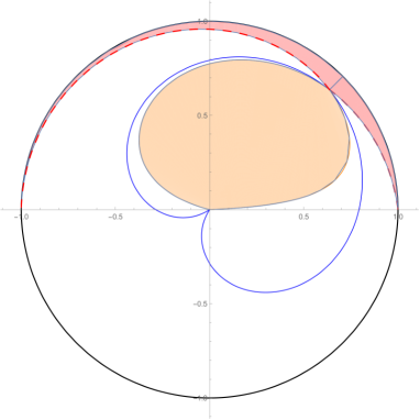
Figure 2: $V_{\mathcal{U}}(0.9e^{i\pi/4})$

3.2 Bounded typically real mappings

Following Rogosinski [Rog32], a holomorphic map $f:\mathbb{D}\to\mathbb{C}$ is called typically real if

$$\text{Im}\,(f(z))\text{Im}\,(z)\geq 0\quad\text{for all $z\in\mathbb{D}.$}$$

Now we define $\mathcal{T}$ as the set of all typically real self-mappings $f:\mathbb{D}\to\mathbb{D}$ with $f(0)=0$ and $f^{\prime}(0)>0$. Obviously, $\mathcal{U}\subset\mathcal{T}.$
From Rogosinski’s work one immediately obtains an integral representation for typically real mappings, see also [Rob35], Section 2. In order to determine the value region $V_{\mathcal{T}}(z_{0})$, we will need the following integral representation for bounded typically real mappings.

Theorem 3.4 ([SS82], Theorem 2.2).

Let $f\in\mathcal{T}$ with $f^{\prime}(0)=\tau>0.$ Then there exists a probability measure $\mu$ supported on $B:=\{(x,y)\in\mathbb{R}^{2}\,|\,-1\leq x\leq 2\tau-1\leq y\leq 1\}$ such that

$$f(z)=\frac{\sqrt{g_{\mu,\tau}(z)}-1}{\sqrt{g_{\mu,\tau}(z)}+1},$$

where we take the holomorphic branch of the square root with $\sqrt{1}=1$ and

$$g_{\mu,\tau}(z)=\int_{B}\frac{(1+z)^{2}(1-2(1-2\tau+x+y)z+z^{2})}{(1-2xz+z^{2})(1-2yz+z^{2})}\,\mu(dxdy).$$

Remark 3.5.

In order to show $\mathcal{U}\subsetneq\mathcal{T}$ we find a function $f_{0}\in\mathcal{T}\setminus\mathcal{U}$ as follows: Let $\tau=1/2$ and let $\mu$ be the point measure in $(\tau-1,\tau).$ Then we obtain

$$f_{0}(z)=\frac{\sqrt{((1+z)^{2}(1+z^{2}))/(1+z^{2}+z^{4})}-1}{\sqrt{((1+z)^{2}(1+z^{2}))/(1+z^{2}+z^{4})}+1}.$$

The derivative $f_{0}^{\prime}(z)$ has a zero at $z=-(1/4)+(i\sqrt{3})/4+1/2\sqrt{-(9/2)-(i\sqrt{3})/2}\in\mathbb{D}.$ Hence, $f_{0}\not\in\mathcal{U}.$

Theorem 3.6.

Let $z_{0}\in\mathbb{D}\setminus\{0\}$ and $\tau\in(0,1].$ Define $\mathcal{T}(\tau):=\{f\in\mathcal{T}\,|\,f^{\prime}(0)=\tau\}.$
The set $V_{\mathcal{T}(\tau)}(z_{0})$ is the image of the closed region bounded by the two circular arcs

$$\left\{1+\frac{4\tau z_{0}}{1-2yz_{0}+z_{0}^{2}}\,|\,y\in[2\tau-1,1]\right\}\;\text{and}\;\left\{\frac{(z_{0}+1)^{2}(1+z_{0}(-4+4\tau-2x+z_{0}))}{(z_{0}-1)^{2}(1-2xz_{0}+z_{0}^{2})}\,|\,x\in[-1,2\tau-1]\right\}$$

under the map $w\mapsto\frac{\sqrt{w}-1}{\sqrt{w}+1}.$

Proof.

Fix some $\tau>0$. First we show that the set $A(\tau):=\{g_{\mu,\tau}(z_{0})\,|\,\text{$\mu$ is a point measure on $B$}\}$ is convex. To this end, we evaluate the function $(x,y)\mapsto s(x,y):=\frac{(1+z)^{2}(1-2(1-2\tau+x+y)z+z^{2})}{(1-2xz+z^{2})(1-2yz+z^{2})}$ on $\partial B:$

• $s(x,y)=\frac{(1+z_{0})^{2}}{(z_{0}+1)^{2}-4\tau z_{0}}$ when $x=2\tau-1.$

• $s(x,y)=\frac{(1+z_{0})^{2}}{(z_{0}+1)^{2}-4\tau z_{0}}$ when $y=2\tau-1.$

• $s(x,y)=1+\frac{4\tau z_{0}}{1-2yz_{0}+z_{0}^{2}}$ when $x=-1.$

• $s(x,y)=\frac{(z_{0}+1)^{2}(1+z_{0}(-4+4\tau-2x+z_{0}))}{(z_{0}-1)^{2}(1-2xz_{0}+z_{0}^{2})}$ when $y=1$.

We see that $s(\partial B)$ consists of two circular arcs connecting the points

$$P(\tau)=\frac{(1+z_{0})^{2}}{(1+z_{0})^{2}-4\tau z_{0}}\quad\text{and}\quad Q(\tau)=1+\frac{4\tau z_{0}}{1-2z_{0}+z_{0}^{2}},$$ (3.1)

and the two arcs are given by

$$s_{1,\tau} :[2\tau-1,1]\to\mathbb{C},\quad s_{1,\tau}(y):=1+\frac{4\tau z_{0}}{1-2yz_{0}+z_{0}^{2}},$$

$$s_{2,\tau} :[-1,2\tau-1]\to\mathbb{C},\quad s_{2,\tau}(x):=\frac{(z_{0}+1)^{2}(1+z_{0}(-4+4\tau-2x+z_{0}))}{(z_{0}-1)^{2}(1-2xz_{0}+z_{0}^{2})}.$$

Without loss of generality we restrict to the case $\text{Im}\,(z_{0})\geq 0.$
A short calculations shows that then

$$\frac{d}{dy}\arg\frac{d}{dy}s(x,y) =4\text{Im}\,z_{0}\frac{1-|z_{0}|^{2}}{|1-2yz_{0}+z_{0}^{2}|^{2}}\geq 0,$$

$$\frac{d}{dx}\arg\frac{d}{dx}s(x,y) =4\text{Im}\,z_{0}\frac{1-|z_{0}|^{2}}{|1-2xz_{0}+z_{0}^{2}|^{2}}\geq 0.$$

Furthermore, we have

$$s_{x}(x,y):=\frac{d}{dx}s(x,y) =\frac{4(2\tau-1-y)z^{2}(1+z)^{2}}{(1-2xz+z^{2})^{2}(1-2yz+z^{2})},$$

$$s_{y}(x,y):=\frac{d}{dy}s(x,y) =\frac{4(2\tau-1-x)z^{2}(1+z)^{2}}{(1-2yz+z^{2})^{2}(1-2xz+z^{2})},$$

and thus

$$\text{Im}\,\frac{s_{x}(x,y)}{s_{y}(x,y)}=\frac{2(y-(2\tau-1))}{2\tau-1-x}\frac{1-|z|^{2}}{|1-2xz+z^{2}|^{2}}\text{Im}\,(z)\cdot(y-x)\geq 0$$ (3.2)

for all $(x,y)\in B.$
This shows that any parallel to either the $x$- or the $y$-axis within $B$ is mapped onto a convex curve, and that whenever we map a path that points inwards in $B$, the image also lies in the interior of $s(\partial B)$. Therefore, the convex closure of $A(\tau)$ is equal to the set $W(\tau)$ defined as the compact region bounded by the curves $s_{1,\tau}$ and $s_{2,\tau}$.
From Theorem 3.4 it follows that $V_{\mathcal{T}(\tau)}(z_{0})$ is the image of $K(\tau):=\{g_{\mu,\tau}(z_{0})\,|\,\text{$\mu$ prob. meas. on $B$}\}$ under the map $w\mapsto\frac{\sqrt{w}-1}{\sqrt{w}+1}.$ The set $K(\tau)$ is the closure of the convex hull of $A(\tau),$ i.e. $K(\tau)=W(\tau)$, which concludes the proof.

∎

Figure 3 shows the set $V_{\mathcal{T}(\tau)}(z_{0})$ for $z_{0}=0.9e^{i\pi/4}$ and $\tau=0.1,0.5,0.9$ (shaded regions).

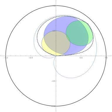
Figure 3: $V_{\mathcal{T}(\tau)}(z_{0})$.

Corollary 3.7.

Let $z_{0}\in\mathbb{D}\setminus\{0\}.$ Then $V_{\mathcal{T}}(z_{0})=V_{\mathcal{U}}(z_{0}).$
Furthermore, if $z_{0}\not\in\mathbb{R}$, then each $w\in\partial V_{\mathcal{T}}(z_{0})$ except $0$ can be reached by only one mapping $f\in\mathcal{T}$, which is of the form $f_{1,t}$ or $f_{2,t}$ from Theorem 3.1.

Proof.

Again, we denote by $W(\tau)$ the image of $V_{\mathcal{T}(\tau)}(z_{0})$ under the map $z\mapsto(1+z)^{2}/(1-z)^{2},$ the inverse function of $w\mapsto\frac{\sqrt{w}-1}{\sqrt{w}+1},$ which is the convex region bounded by the circular arcs $s_{1,\tau}(y),$ $y\in[2\tau-1,1],$ and $s_{2,\tau}(x),$ $x\in[-1,2\tau-1].$
Consider the convex region $R$ bounded by the circular arc

$$C:=\left\{P(\tau)\,|\,\tau\in[0,1]\right\}\text{ and the line segment }L:=\left\{Q(\tau)\,|\,\tau\in[0,1]\right\}, *$$ ()

where $Q(\tau)$ and $P(\tau)$ are defined as in (3.1).

Fix $\tau\in(0,1].$ To show that $W(\tau)$ is contained in $R$, assume the opposite. Then the boundary of $W(\tau)$ has to intersect either $C$ or $L$ in some other point besides $P(\tau)$ and $Q(\tau).$ However, it is easy to see that each of the following four equations

$$s_{1,\tau}(y) =P(t),\quad y,t\in\mathbb{R},$$

$$s_{1,\tau}(y) =Q(t),\quad y,t\in\mathbb{R},$$

$$s_{2,\tau}(x) =P(t),\quad x,t\in\mathbb{R},$$

$$s_{2,\tau}(x) =Q(t),\quad x,t\in\mathbb{R},$$

has only one solution, namely $(y,t)=(1,\tau),$ $(y,t)=(2\tau-1,\tau),$ $(x,t)=(-1,\tau),$ and $(x,t)=(2\tau-1,\tau)$, respectively. (In all four cases, the second intersection point between the circles/lines is given by the limit cases $y\to\infty$ and $x\to\infty$ respectively.)

Hence, we have $W(\tau)\subset R$ for every $\tau\in(0,1].$ Finally, it is clear that every point contained in $R\setminus\{1\}$ (note that $P(0)=Q(0)=1$) is contained in some $W(\tau)$: since every $W(\tau)$ is convex, the line segment between $P(\tau)$ and $Q(\tau)$ is always contained in $W(\tau)$.
Consequently, $\cup_{\tau\in(0,1]}W(\tau)=R\setminus\{1\}.$

Now we apply the function $z\mapsto(1+z)^{2}/(1-z)^{2},$ the inverse function of $w\mapsto\frac{\sqrt{w}-1}{\sqrt{w}+1},$ to the curves $C_{+}(z_{0})$ and $C_{-}(z_{0})$ from Theorem 3.1 and we obtain the curves

$$\left\{\frac{(1+z_{0})^{2}}{(1+z_{0})^{2}-4e^{-t}z_{0}}\,|\,t\in[0,\infty]\right\}\text{ and }\left\{1+\frac{4e^{-t}z_{0}}{(z_{0}-1)^{2}}\,|\,t\in[0,\infty]\right\},$$

which are the very same curves as ($*$ ‣ 3.2). Thus, we conclude that $V_{\mathcal{T}}(z_{0})=V_{\mathcal{U}}(z_{0})$.

Finally, assume $z_{0}\not\in\mathbb{R}$ and let $w\in\partial V_{\mathcal{T}}(z_{0})\setminus\{0\}.$ Then $w=P(\tau)$ or $w=Q(\tau)$ for a unique $\tau\in(0,1]$ and the proof of Theorem 3.6 shows that there is only one mapping $f\in V_{\mathcal{T}(\tau)}(z_{0})$ with $f(z_{0})=w.$ From Theorem 3.1 it follows that $f$ is of the form $f_{1,t}$ or $f_{2,t}.$ ∎

3.3 Real coefficients

Finally we take a look at one further value region, determined by Rogosinski in [Rog34], p.111: Let $\mathcal{R}$ be the set of all holomorphic functions $f:\mathbb{D}\to\mathbb{D}$ with $f(0)=0$ that have only real coefficients in the power series expansion around 0. Then $V_{\mathcal{R}}(z_{0})$ is the intersection of the two closed discs whose boundaries are the circles through $1,z_{0},-z_{0}$ and through $-1,-z_{0},z_{0}$ respectively.

Let $\mathcal{R}^{\geq}$ be the set of all holomorphic functions $f\in\mathcal{R}$ with $f^{\prime}(0)\geq 0$ and $z_{0}\in\mathbb{D}\setminus\{0\}.$ Then we have

$$V_{\mathcal{T}}(z_{0})\subset V_{\mathcal{R}^{\geq}}(z_{0})\subset V_{\mathcal{R}}(z_{0}).$$

It is clear that $V_{\mathcal{R}^{\geq}}(z_{0})\not=V_{\mathcal{R}}(z_{0})$ as the point $-z_{0}$ belongs to $V_{\mathcal{R}}(z_{0})$ and there is only one mapping $f\in\mathcal{R}(z_{0})$ with $f(z_{0})=-z_{0}$, namely $f(z)=-z$ for all $z\in\mathbb{D}.$
Furthermore, if $z_{0}\not\in\mathbb{R},$ we have $V_{\mathcal{T}}(z_{0})\subsetneq V_{\mathcal{R}^{\geq}}(z_{0})$ which can be seen as follows: The boundary points of $V_{\mathcal{R}}(z_{0})$ can be reached only by the functions $z\mapsto\pm z\frac{z-x}{zx-1},$ $x\in[-1,1],$ see [Rog34], p.111. Hence, by Corollary 3.7 we have $\partial V_{\mathcal{T}}(z_{0})\cap\partial V_{\mathcal{R}}(z_{0})=\{z_{0}\}.$ For $0<x<1$, the function $f(z)=z\frac{z-x}{zx-1}$ satisfies $f^{\prime}(0)=x>0$ and $f(z_{0})\not=z_{0}.$ This gives us $z_{0}\frac{z_{0}-x}{z_{0}x-1}\in V_{\mathcal{R}^{\geq}}(z_{0})\setminus V_{\mathcal{T}}(z_{0}).$

Theorem 3.8.

Let $z_{0}\in\mathbb{D}\setminus\{0\}.$ Then $V_{\mathcal{R}^{\geq}}(z_{0})$ is the closed convex region bounded by the following three curves:

$$A = \left\{z_{0}\frac{z_{0}-x}{z_{0}x-1}\,\big{|}\,x\in[0,1]\right\},\quad B=\left\{z_{0}\frac{z_{0}+x}{z_{0}x+1}\,\big{|}\,x\in[0,1]\right\},$$

$$C = \left\{\frac{z_{0}^{2}(z_{0}+2x-1)}{1+2xz_{0}-z_{0}}\,\big{|}\,x\in[0,1]\right\}.$$

Proof.

Let $f\in\mathcal{R}^{\geq}.$ Then $g(z):=(1+f(z))/(1-f(z))$ maps $\mathbb{D}$ into the right half-plane with $g(0)=1$, $g$ has only real coefficients in its power series expansion around $0$ and $g^{\prime}(0)=2f^{\prime}(0)\geq 0.$ Due to the Herglotz representation ([Dur83], Section 1.9) we can write $g$ as

$$g(z)=\int_{\partial\mathbb{D}}\frac{u+z}{u-z}\,\nu(du),$$ (3.3)

for some probability measure $\nu$ on $\partial\mathbb{D}.$
As $g$, and thus $\nu$, is symmetric with respect to the real axis, one can rewrite (3.3) as

$$g(z)=\int_{\partial\mathbb{D}}1/2\frac{u+z}{u-z}+1/2\frac{\overline{u}+z}{\overline{u}-z}\,\nu(du)=\int_{\partial\mathbb{D}}\frac{1-z^{2}}{1-2z\text{Re}(u)+z^{2}}\,\nu(du),$$ (3.4)

or

$$g(z)=G_{\mu}(z):=\int_{[0,\pi]}\frac{1-z^{2}}{1-2z\cos(u)+z^{2}}\,\mu(du),$$ (3.5)

where $\mu$ is a probability measure on $[0,\pi]$ that additionally fulfils

$$\int_{[0,\pi]}\cos(u)\,\mu(du)\geq 0,$$ (3.6)

as the last integral is equal to $g^{\prime}(0)/2=f^{\prime}(0).$ Thus we need to determine the extreme points of the convex set of all measures on $[0,\pi]$ that satisfy (3.6). According to [Win88], Theorem 2.1, this set of extreme points is contained in the set $S$ that consists of all point measures $\mu=\delta_{\phi}$ on $[0,\pi]$ satisfying (3.6) and of all convex combinations $\mu=\lambda\delta_{\phi}+(1-\lambda)\delta_{\varphi}$, with $\phi,\varphi\in[0,\pi]$, $\phi\not=\varphi,$ $\lambda\in(0,1),$ satisfying (3.6).

We can now determine $V_{\mathcal{R}^{\geq}}(z_{0})$ as follows: Denote by $W_{\mathcal{R}^{\geq}}(z_{0})$ the image of $V_{\mathcal{R}^{\geq}}(z_{0})$ under the injective map $w\mapsto(1+w)/(1-w).$ Then $W_{\mathcal{R}^{\geq}}(z_{0})$ is the closure of the convex hull of the set $\{G_{\mu}(z_{0})\,|\,\mu\in S\}.$

The point measures from $S$ are, of course, all $\delta_{\phi}$ with $\phi\in[0,\pi/2],$ and (3.5) gives us the curve

$$\frac{1-z_{0}^{2}}{1-2z_{0}x+z_{0}^{2}},\quad x\in[0,1],$$ (3.7)

a circular arc connecting the points $\frac{1-z_{0}^{2}}{1+z_{0}^{2}}$ and $\frac{1+z_{0}}{1-z_{0}}.$ This curve is the image of $A$ under the map $w\mapsto\frac{1+w}{1-w}.$ The image of $B$ is the line segment

$$\frac{1+2xz_{0}+z_{0}^{2}}{1-z_{0}^{2}},\quad x\in[0,1],$$ (3.8)

which connects $\frac{1+z_{0}^{2}}{1-z_{0}^{2}}$ to $\frac{1+z_{0}}{1-z_{0}}.$

The other measures have the form $\lambda\delta_{\phi}+(1-\lambda)\delta_{\varphi}$ with w.l.o.g. $\phi\in[0,\pi/2],$ $\varphi\in[0,\pi]$, $\phi\not=\varphi$, $\lambda\in(0,1)$ such that $\lambda\cos(\phi)+(1-\lambda)\cos(\varphi)\geq 0.$ They lead to the set

$$\lambda\frac{1-z_{0}^{2}}{1-2z_{0}x+z_{0}^{2}}+(1-\lambda)\frac{1-z_{0}^{2}}{1-2z_{0}y+z_{0}^{2}},\quad x\in[0,1],y\in[-1,1],\lambda\in(0,1),\lambda x+(1-\lambda)y\geq 0.$$ (3.9)

If we take $x=1,$ $y\in[-1,0]$ and $\lambda=\frac{y}{y-1}$ (which is equivalent to $\lambda+(1-\lambda)y=0$), then we obtain

$$\frac{(1+z_{0})(1-2(1+y)z_{0}+z_{0}^{2})}{(1-z_{0})(1-2yz_{0}+z_{0}^{2})}.$$ (3.10)

The above expression describes a circular arc connecting the points $\frac{1+z_{0}^{2}}{1-z_{0}^{2}}$ and $\frac{1-z_{0}^{2}}{1+z_{0}^{2}}$, and this arc is the image of the curve $C$ under the map $w\mapsto\frac{1+w}{1-w}.$ Note that the point $\frac{1+z_{0}}{1-z_{0}}$ lies on the full circle, which is obtained when $y\to\infty.$
Denote by $\Delta$ the closed bounded region bounded by the three curves (3.7), (3.8) and (3.10). Then $\Delta$ is convex. We are done if we can show that for all other measures from (3.9), $G_{\mu}(z_{0})$ belongs to $\Delta.$ Then we can conclude that $\Delta$ is the closure of the convex hull of $\{G_{\mu}(z_{0})\,|\,\mu\in S\}.$

First, we consider the points from (3.9) for $x\in[0,1],$ $y\in[-1,0]$ and again $\lambda=\frac{y}{y-x}:$

• For $y=1,$ we obtain the curve

  $$-\frac{(-1+z_{0})(1+z_{0}(2-2x+z_{0}))}{(1+z_{0})(1-2xz_{0}+z_{0}^{2})},\quad x\in[0,1].$$ (3.11)

  Like the curve (3.10), this arc also connects $\frac{1+z_{0}^{2}}{1-z_{0}^{2}}$ and $\frac{1-z_{0}^{2}}{1+z_{0}^{2}}$. For $x\to\infty$ we obtain $\frac{1-z_{0}}{1+z_{0}}$, which is the second intersection point of the full circles corresponding to (3.7) and (3.8) (note that this point is mapped onto $-z_{0}$ under $w\mapsto\frac{1+w}{1-w}$). We conclude that (3.11) is contained in $\Delta.$ The convex set bounded by (3.10) and (3.11) will be denoted by $\Delta_{0}$, and is, of course, contained in $\Delta.$ (Figure 5 shows the image of $\Delta_{0}$ under the map $w\mapsto\frac{1+w}{1-w}$.)

• Now fix $x\in[0,1)$ and (3.9) becomes

  $$\frac{(-1+z_{0}^{2})(1-2(x+y)z_{0}+z_{0}^{2})}{(-1+2xz_{0}-z_{0}^{2})(1-2yz_{0}+z_{0}^{2})},\quad y\in[0,1].$$ (3.12)

  This set is a circular arc connecting $\frac{1-z_{0}^{2}}{1+z_{0}^{2}}$ ($y=0$) to a point on (3.11) ($y=1$). For $y\to\infty$ we obtain the point $\frac{1-z_{0}^{2}}{1-2xz_{0}+z_{0}^{2}}$, which lies on (3.7) and is not contained in $\Delta_{0}.$ We conclude that the arc (3.12) lies within $\Delta_{0}$ and thus in $\Delta.$

Finally, assume there are $x\in[0,1],y\in[-1,1],\lambda\in(0,1)$ such that $\lambda x+(1-\lambda)y>0$ (i.e. $G_{\mu}^{\prime}(0)>0$) and the corresponding point (3.9) lies outside $\Delta.$ Since it has nevertheless to lie in $V_{\mathcal{R}}(z_{0})$, the line segment between this point and $\frac{1+z_{0}}{1-z_{0}}$ must intersect the curve (3.10). Thus, the set $\{f(z_{0})\,|\,f\in\mathcal{R},f^{\prime}(0)>0\}$, which doesn’t contain the curve $C$, could not be convex, a contradiction.

∎

The sets $V_{\mathcal{T}}(z_{0})$ (orange), $V_{\mathcal{R}^{\geq}}(z_{0})$ (red) and $V_{\mathcal{R}}(z_{0})$ (green) are shown in Figure 5 for $z_{0}=\frac{1}{3}+\frac{i}{2}.$

            Figure 4: $V_{\mathcal{T}}(z_{0}),V_{\mathcal{R}^{\geq}}(z_{0}),V_{\mathcal{R}}(z_{0})$.             Figure 5: $\Delta_{0}.$

Corollary 3.9.

Let $\mathcal{R}^{0}=\{f\in\mathcal{R}^{\geq}\,|\,f^{\prime}(0)=0\}$ and $z_{0}\in\mathbb{D}\setminus\{0\}.$ Then $V_{\mathcal{R}^{0}}(z_{0})=\Delta_{0},$ i.e. $V_{\mathcal{R}^{0}}(z_{0})$ is the closed convex set bounded by the circular arcs $C$ and $-C$, which intersect at $z_{0}^{2}$ and $-z_{0}^{2}.$

Proof.

We can proceed as in the proof of Theorem 3.8. Condition (3.6) then has to be replaced by

$$\int_{[0,\pi]}\cos(u)\,\mu(du)=0,\text{ which we can also write as}$$ (3.13)

$$\int_{[0,\pi]}\cos(u)\,\mu(du)\geq 0\text{ and }\int_{[0,\pi]}\cos(u)\,\mu(du)\leq 0$$

in order to apply again [Win88], Theorem 2.1. Then we obtain that the image of $V_{\mathcal{R}^{0}}(z_{0})$ under the map $w\mapsto(1+w)/(1-w)$ is equal to the closure of the convex hull of the set $\{G_{\mu}(z_{0})\,|\,\mu\in S,\mu\text{ satisfies \eqref{workhard2}}\}.$

The proof of Theorem 3.8 shows that this set is equal to $\Delta_{0}.$ ∎

Corollary 3.10.

Let $\mathcal{R}^{>}=\{f\in\mathcal{R}^{\geq}\,|\,f^{\prime}(0)>0\}$ and $z_{0}\in\mathbb{D}\setminus\{0\}.$ Then $V_{\mathcal{R}^{>}}(z_{0})=V_{\mathcal{R}^{\geq}}(z_{0})\setminus C,$ where $C$ is the curve from Theorem 3.8.

Proof.

Obviously, the curves $A$ and $B$ from Theorem 3.8 minus their endpoint $z_{0}^{2}$ and $-z_{0}^{2}$ belong to $V_{\mathcal{R}^{>}}(z_{0}).$ The curve $C$ does not belong to the set $V_{\mathcal{R}^{>}}(z_{0})$, but it belongs to its closure, which can be seen by approximating the curve by points from (3.9) for $\lambda=\frac{y-1/n}{y-x},$ $n\in\mathbb{N},$ which means the integral in (3.6) is equal to $1/n$ in this case.
As $V_{\mathcal{R}^{>}}(z_{0})$ is a convex set, we conclude that $V_{\mathcal{R}^{>}}(z_{0})$ is equal to $V_{\mathcal{R}^{\geq}}(z_{0})\setminus C.$

∎

References

- [Dur83] P. L. Duren, Univalent functions, Springer-Verlag, New York, 1983.
- [GB92] V. V. Goryainov and I. Ba, Semigroup of conformal mappings of the upper half-plane into itself with hydrodynamic normalization at infinity, Ukraine. Mat. Zh. 44 (1992), no. 10, 1320–1329.
- [Gor86] V. V. Goryainov, Semigroups of conformal mappings, Mat. Sb. (N.S.), 129(171):4 (1986), 451– 472.
- [Gor15] V. V. Goryainov, Evolution families of conformal mappings with fixed points and the Löwner-Kufarev equation, Mat. Sb., 206:1 (2015), 39 – 68.
- [KS16] J. Koch and S. Schleißinger, Value ranges of univalent self-mappings of the unit disc, J. Math. Anal. Appl. 433 (2016), no. 2, 1772–1789.
- [Pfr16] D. Pfrang, Der Wertebereich typisch-reeller schlichter beschränkter Funktionen, Master thesis, University of Würzburg, 2016.
- [Pro92] D. V. Prokhorov, The set of values of bounded univalent functions with real coefficients, Theory of functions and approximations, Part 1 (Russian) (Saratov, 1990), Izdat. Saratov. Univ. (1992), 56–60.
- [PS16] D. V. Prokhorov and K. Samsonova, A Description Method in the Value Region Problem, Complex Analysis and Operator Theory (2016).
- [Rob35] M. S. Robertson, On the coefficients of a typically-real function, Bull. Amer. Math. Soc., Volume 41, Number 8 (1935), 565–572.
- [Rog32] W. Rogosinski, Über positive harmonische Entwicklungen und typisch-reelle Potenzreihen., Math. Z. 35 (1932), 93–121.
- [Rog34] W. Rogosinski, Zum Schwarzschen Lemma., Jahresber. Dtsch. Math.-Ver. 44 (1934), 258–261.
- [RS14] O. Roth and S. Schleißinger, Rogosinski’s lemma for univalent functions, hyperbolic Archimedean spirals and the Loewner equation, Bull. Lond. Math. Soc. 46 (2014), no. 5, 1099–1109.
- [SS82] M. Szapiel and W. Szapiel, Extreme points of convex sets. IV. Bounded typically real functions, Bull. Acad. Polon. Sci. Sér. Sci. Math. 30 (1982), no. 1-2, 49-57.
- [Tam78] O. Tammi, Extremum Problems for Bounded Univalent Functions, Springer, Berlin-New York, 1978.
- [Win88] G. Winkler, Extreme points of moment sets, Math. Oper. Res. 13 (1988), no. 4, 581–587.