Nuclear dynamics investigation of the initial electron transfer in the cyclobutane pyrimidine dimer lesion repair process by photolyases

Abstract

Photolyases are proteins capable of harvesting the sunlight to repair DNA damages caused by UV light. In this work we focus on the first step in the repair process of the cyclobutane pyrimidine dimer photoproduct (CPD) lesion, which is an electron transfer (ET) from a flavine cofactor to CPD, and study the role of various nuclear degrees of freedom (DOF) in this step. The ET step has been experimentally studied using transient spectroscopy and the corresponding data provide excellent basis for testing the quality of quantum dynamical models. Based on previous theoretical studies of electronic structure and conformations of the protein active site, we present a procedure to build a diabatic Hamiltonian for simulating the ET reaction in a molecular complex mimicking the enzyme’s active site. We generate a reduced nuclear dimensional model that provides a first non-empirical quantum dynamical description of the structural features influencing the ET rate. By varying the nuclear DOF parametrization in the model to assess the role of different nuclear motions, we demonstrate that the low frequency flavin butterfly bending mode slows ET by reducing Franck-Condon overlaps between donor and acceptor states and also induces decoherence.

I Introduction

UV radiation causes damage to DNA by forming bonds between contiguous thymine bases. There are two types of such lesions: the cyclobutane pyrimidine dimer photoproduct (CPD) and the pyrimidine-pyrimidone (6-4) photoproduct. Both lesions can be repaired by flavoproteins: photolyases (PLs) that are capable of splitting the thymine dimers back to monomers. Sancar (2003, 2008); Müller and Carell (2009) While PLs are not present in Humans, they have been found in bacteria, fungi, plants and animals, Sancar (2003) these proteins proved to be useful in protection against sunburns and skin cancer prevention when added to sunscreens. Berardesca et al. (2012); Emanuele et al. (2013); Emanuele, Spencer, and Braun (2014) Understanding the molecular-level details of the repair processes is of high interest not only for our basic knowledge, but also for the potential improvement of the efficiency of such treatments or for drug design. Theoretical models are required to unravel microscopic mechanisms at work in the PL s’ active site by comparison of the model predictions with the available experimental measurements. In this paper we present a methodology to construct such quantum dynamical models.

The action of CPD-PL is understood as follows: Mees et al. (2004); Kao et al. (2005) After harvesting the sunlight Weber (2005); Essen and Klar (2006); Zheng, Garcia, and Stuchebrukhov (2008), the protein utilizes the energy excess to break the undesirable bonds between the thymine bases. This process happens due to a cofactor present in the active site of CPD-PL: a flavine adenine dinucleotide (FAD). FAD consists of riboflavin connected to adenosine by two phosphates.

Due to reduction of the isoalloxazine ring of riboflavin (lumiflavin in Fig. 1), the FAD cofactor is present in either two redox states: FADH^- or FADH^∙. The importance of the FAD cofactor is in its role of electron donor to the pyrimidine dimer to initiate the repair process. The repair process includes the following steps: Kao et al. (2005) 1) light excitation of a flavin-type antenna cofactor, 7,8-didemethyl-8-hydroxy-5-deazariboflavin, 2) energy transfer to the FAD H^-, 3) forward electron transfer (ET) from excited FAD H^- to the thymine dimer, 4) bond dissociations, 5) electron back transfer to FAD H^∙.

Figure 1: a) Minimal molecular model for the CPD-PL active site. b) Chemical structure of the CPD. c) chemical structure of lumiflavin in two-electron reduced state and definition of the ’butterfly’ bending motion.

The forward ET is a population transfer between a donor state, where the electron is located on excited flavin, and an acceptor state, where the electron is located on CPD. The lifetime of the ET reaction has been measured to be $170$ ps by transient absorption experiments at room temperature. Kao et al. (2005); Liu et al. (2012) Such a long timescale indicates a small coupling between the two electronic states, which is supported by the first estimate of this coupling in Ref. 13: $7.10^{-4}$ eV. In this case, the electron is effectively diabatically trapped in the donor state.Blancafort et al. (2001); Blancafort, Hunt, and Robb (2005) It was found recently that capturing quantum interference in the nuclear wavefunction can be crucial for adequate modelling of such systems.Joubert-Doriol, Ryabinkin, and Izmaylov (2013) Therefore, a fully quantum treatment of the nuclear motion using vibronic models appears to be necessary. However, building a vibronic model for systems of our interest leads to another major difficultie, which is the large number of nuclear degrees of freedom (DOF), over one hundred that are involved in the ET process. To address these challenges in an adequate and computationally feasible way we use a perturbative approach, which is an extension to the usual Fermi Golden Rule: Borrelli and Peluso (2011, 2015) the non-equilibrium Fermi golden rule (NFGR). Izmaylov et al. (2011); Endicott, Joubert-Doriol, and Izmaylov (2014)

The NFGR method scales only cubically Endicott, Joubert-Doriol, and Izmaylov (2014) with the number of DOF in the calculation of the time evolution of the donor state population and. Therefore, NFGR seems well suited to treat ETs in large systems. There are two conditions for NFGR success: 1) a small coupling between donor and acceptor states for applicability of the perturbation theory, and 2) small amplitude motions, since the method employs the harmonic approximation with rectilinear coordinates for the nuclear coordinate. Here, both conditions are assumed to be satisfied. The first, because of the very long time scale of the ET. The second, because the protein environment constrains the relative motion of FAD H^- and CPD. Liu et al. (2013) The NFGR method requires a diabatic representation of the Hamiltonian Izmaylov et al. (2011); Endicott, Joubert-Doriol, and Izmaylov (2014) built based on the first-principles electronic structure calculations. Here, we apply a diabatization by ansatz to minimize non-adiabatic couplings. Cederbaum, Köppel, and Domcke (1981); Köppel, Domcke, and Cederbaum (1984); Joubert-Doriol et al. (2014) We construct a diabatic vibronic Hamiltonian model describing the initial ET step occurring in the CPD-PL complex. The model considers two electronic states: donor and acceptor. We employ multi-configurational quantum chemical methods to map the relevant potential energy surfaces (PESs) of the CPD-PL complex Domratcheva (2011), then we optimize model Hamiltonian parameters using the least-square method on electronic state energies.

By using the model outlined above, here we investigate the role of nuclear DOF in the ET process and study their impact on the ET lifetime. We put a special emphasis on a flavin bending (FB) motion that is commonly identified as the flavin butterfly motion and is defined in Fig. 1-c. Two-electron reduced lumiflavin is anti-aromatic and is bent in the middle dihydrodiazine ring where nitrogens have a $sp^{3}$ hybridization in the ground state, Walsh and Miller (2003) while it is found to be planar in excited states. Therefore, the low-frequency FB is believed to play an important role in the non-adiabatic dynamics of the FADH^- cofactor. Kao et al. (2008) On the other hand, the protein environment may constraint the active site and prevent large amplitude motions such as FB. Liu et al. (2013) As detailed below, we observed that the FB motion allows for decoherence and slows down the ET reaction by decreasing Franck-Condon overlaps between the donor and acceptor electronic states.

The rest of the paper is organized as follows. Section II details the methodology. Section III discusses main features of PESs, model variations and ET rate estimates. Section IV concludes the paper and gives an outlook for future applications.

II Methods

II.1 Molecular model and its electronic structure

A molecular model of the active site is taken from Ref. 25 and contains the FADH^- electron donor, modelled by lumiflavin, and the electron acceptor, the CPD lesion of two methylthymines (see Fig. 1). The initial structure of the two moieties is taken from the CPD-PL repair compex crystal structure (PDB file 1TEZ Mees et al. (2004)). In order to simulate geometrical constraints of the protein environment, the nuclear coordinates of the model’s terminal atoms in the model are frozen during geometry optimizations. Thus, these coordinates are not considered in the PESs calculations. After taking into account the geometrical constraints, the final model contains $\mathcal{D}=153$ nuclear (vibrational) DOF. The coordinates of all frozen atoms are given in the supplemental materials. Joubert-Doriol et al. (2015)

Based on previous work in Ref. 25, we use the principal orbital complete active space self consistent field (CASSCF) approach Udvarhelyi and Domratcheva (2011) further improved by the extended multiconfiguration quasi degenerate second order perturbation theory (XMCQDPT2). Granovsky (2011) In this approach, the selected active space contains only the orbitals and electrons necessary to describe the static electron correlation, while XMCQDPT2 accounts for the dynamical electron correlation. At the ground state equilibrium geometry, the active orbitals are: the highest occupied molecular orbital (HOMO), $\pi_{f}$, located on lumiflavin, the lowest unoccupied molecular orbital (LUMO), $\pi_{f}^{*}$, located on lumiflavin, and the antibonding $\pi_{CO}^{*}$ orbital of the closest carbonyl group located on the thymine dimer. This active space gives six electronic configurations. The choice of the active space is guided by an assumption that involvement of out-of-plane deformations of the lumiflavin’s $\pi$-system in the ET process is very limited. Thus, the three active orbitals will not change their character along the entire reaction path and, hence are sufficient for a balanced description of the ET process. The remaining orbitals will mainly only contribute to the dynamic electron correlation energy. The basis set used for the calculations is 6-31G^∗. All active space molecular orbitals are given in the supplemental materials. Joubert-Doriol et al. (2015) Geometry optimization, gradient, and Hessian calculations are performed at the CASSCF level with three-root state-average orbitals. Granovsky (2015) The resulting CASSCF energies are then corrected via XMCQDPT2 computations. Analytic gradients at the XMCQDPT2 level of theory are not yet implemented and numerical gradient would be too cumbersome for such a high dimensional system. For electronic structure calculations we use the Firefly quantum chemistry package, Granovsky which is partially based on the GAMESS (US) Schmidt et al. (1993) source code.

We refer to the ground electronic state $S_{0}$ as the closed shell anionic configuration where two electrons are localized on the lumiflavin $(\pi_{f}^{2})$ orbital. The donor state is the FADH^- excited state, labeled as $S_{D}$, where excess of negative charge is still localized on lumiflavin with the $(\pi_{f}\pi_{f}^{*})$ dominant configuration. The acceptor state, labeled as $S_{A}$, where an extra electron is localized on CPD (the electron transfer state), has the $(\pi_{f}\pi_{CO}^{*})$ dominant configuration.

The states $S_{D}$ and $S_{A}$ are our quasi-diabatic states, which are coupled via potential terms, their crossing gives rise to a conical intersection (CI) between $S_{1}$ and $S_{2}$ in the adiabatic representation. The energy minimum of the CI seam was found by energy minimization constraining the energy difference between states to be zero with the Lagrange multiplier method. Granovsky Currently, there is no implementation of analytic non-adiabatic coupling elements for systems of our size, therefore, an approximate numerical approach was used to obtain these elements. The CASSCF wavefunctions, $\Psi_{j}$, were numerically differentiated considering them as if they were complete active space configuration interaction (CASCI) wavefunctions, i.e. assuming frozen molecular orbitals

$$\left\langle\Psi_{1}\bigg{|}\frac{\partial\Psi_{2}}{\partial R_{\alpha}}\right\rangle \approx \left\langle\Psi_{1}(R_{\alpha})|\Psi_{2}(R_{\alpha}+\Delta R_{\alpha})\right\rangle/{\Delta R_{\alpha}}$$ (1)

$$= \sum_{J=1}^{6}\frac{C^{*}_{1J}(R_{\alpha})C_{2J}(R_{\alpha}+\Delta R_{\alpha})}{\Delta R_{\alpha}}.$$

Here, $R_{\alpha}$ is the $\alpha^{th}$ nuclear coordinate, $C_{jJ}$ is the coefficient in front of the $J^{th}$ configuration state function of the $j^{th}$ electronic state, and $\Delta R_{\alpha}$ is taken to be 0.0115 Å for all nuclear coordinates.

To examine a role of the FB coordinate, two sets of models were generated: model $B$, including the FB coordinate, and model $N$, excluding it. Exclusion of FB is done by optimizing all stationary points at the CASSCF level while constraining the nuclei of all lumiflavin’s $\pi$-conjugated atoms in the lumiflavin plane. All out-of-plane coordinates of corresponding atoms have been fixed at their values found in minimizing the first excited state with respect to nuclear positions without constraints. Hence, removing the single FB coordinate is done by removing a collection of fourteen rectilinear coordinates.

II.2 Diabatic model

Our model vibronic Hamiltonians are parametrized using the quadratic vibronic coupling (QVC) form Köppel, Yarkony, and Barentzen (2010) containing two electronic states

$$H = \begin{pmatrix}H_{D}&V_{c}\\ V_{c}&H_{A}\end{pmatrix},$$ (2)

where $H_{D}$ and $H_{A}$ are the individual vibronic Hamiltonians of $S_{D}$ and $S_{A}$, and $V_{c}$ is the vibronic coupling between the two electronic states:

$$H_{k} = -\frac{1}{2}\sum_{\alpha}^{\mathcal{D}}\frac{\partial_{\alpha}^{2}}{\partial x_{\alpha}^{2}}+V_{k}\hskip 9.95863pt\{k=D,A\},$$

$$V_{k} = E_{k}+\sum_{\alpha}^{\mathcal{D}}v_{k,\alpha}x_{\alpha}+\sum_{\alpha,\beta}^{\mathcal{D}}x_{\alpha}K_{k,\alpha\beta}x_{\beta}\hskip 9.95863pt\{k=D,A,c\},$$

$x_{\alpha}$ is the $\alpha^{th}$ mass-weighted nuclear coordinate, $E_{k}$, $v_{k,\alpha}$, and $K_{k,\alpha\beta}$ are real-valued parameters used in the second order expansion of the model. The subscript $k$ takes values $D$, $A$, and $c$ to denote donor, acceptor, and coupling terms respectively. $2K_{k,\alpha\beta}$ represent the Hessian of the diabatic term $k$. We use atomic units in Eq. (2) and throughout the paper. Boldface letters denote vectors and matrices quantities, for example, the matrix $K_{k,\alpha\beta}$ is written $\bm{K}_{k}$. All models represent bound quantum systems which imposes some constraints on parametrization of the matrices $\bm{K}_{k}$ and is further elaborated in App. A. Any diabatic model can be transformed by a unitary transformation and will give the same dynamics. The DOF associated with this unitary transformation are redundant and fixed by imposing a real parametrization as in Eq. (2) and by imposing $E_{c}=0$, which implies that diabatic and adiabatic states are matching at the coordinate origin.

There are about 36,000 parameters for the full dimensional model $B$ and about 30,000 for model $N$. Therefore, usual fitting methods for adiabatic energies represented on a grid of points such as Levenberg-Marquardt Levenberg (1944); Marquardt (1963) cannot be used here because the Jacobian and numerical gradients calculations in the parameter space are too cumbersome. Instead, we developed a two-step approach:

1) We generate a five-dimensional (5D) QVC model for a primary system of the most important modes. The selected five primary modes correspond to the three vectors connecting the most important geometries of the molecular model (three minima of electronic states and the CI seam minumum) and the two branching space vectors at the minimum of the CI seam. The corresponding Hamiltonian is $H_{pri}$ and is parametrized accroding to Eq. (2). Parameters of $H_{pri}$ are optimized in order to minimize the root mean square deviation (RMSD) of the adiabatic energies on a set of grid points along the primary modes. The optimization is done using the simplex algorithm. Nelder and Mead (1965) To suppress the appearance of negative curvatures in the diabatic states during the parameter optimization they have been assigned extra weights in a penalty function. For this optimization, the resulting models’ RMSDs are smaller than $2.4\cdot 10^{-2}$ eV.

2) The remaining secondary modes constitute a secondary system with a Hamiltonian $H_{sec}$. They are included to build the full-dimensional model with a Hamiltonian

$$H_{ful} = H_{pri}+H_{sec}$$ (4)

where $H_{pri}$ has been defined at the previous step and $H_{ful}$ is parametrized accroding to Eq. (2). $H_{sec}$ parameters are obtained using the steepest descent algorithm detailed in App. B. Resulting models’ RMSDs are smaller than $3\cdot 10^{-3}$ eV Bohr^-1m${}_{e}^{-1/2}$ for the fitting of the linear terms and smaller than $2.5\cdot 10^{-4}$ eV Bohr^-2m${}_{e}^{-1}$ for the fitting of the quadratic terms. All directions corresponding to negative curvatures in the diabatic state Hessians of $H_{sec}$ have been removed. Using this two step procedure, two primary system models have been generated: the $B_{pri}$ model that includes the FB coordinate, and the $N_{pri}$ model without the FB coordinate. The corresponding full-dimensional models are labeled $B_{ful}$ and $N_{ful}$, and have dimensionalities of $\mathcal{D}=109$ and $\mathcal{D}=105$, respectively.

The electronic structure calculations for these fittings are done at the CASSCF level. The dynamical electron correlation is then included in the diabatic model by adjusting constant and linear terms of diabatic Hamiltonians to match the XMCQDPT2 energies on a set of grid points connecting the stationary points. This step is motivated by the fact that the quasi-diabatic states correspond to a dominant configuration or a set of configurations represented by a particular element of the diabatic Hamiltonian, on which the XMCQDPT2 correction will have a uniform effect for all nuclear geometries. This correction can be done only for primary system models because such a grid cannot be built for the full dimensional space. This correction was applied on model $B_{pri}$.

II.3 Lifetime calculation

The electron transfer dynamics is followed as the population of the the donor state with the NFGR method. Izmaylov et al. (2011); Endicott, Joubert-Doriol, and Izmaylov (2014) The population of the donor state is expressed as

$$P_{D}(t) = \left\langle D\left|\operatorname{Tr}_{B}\{\rho(t)\}\right|D\right\rangle$$ (5)

$$= \left\langle D\left|\operatorname{Tr}_{B}\{\Lambda(t)\rho(0)\Lambda(t)^{\dagger}\}\right|D\right\rangle,$$

where $\operatorname{Tr}_{B}\{\dots\}$ is the trace over all model nuclear DOF, $\left|D\right\rangle$ is the donor electronic state, $\rho(t)$ is the total density matrix of the quantum system at time $t$, and $\Lambda(t)$ is the unitary evolution operator. Under the assumption that the coupling element $V_{c}$ is small, $\Lambda(t)$ can be expanded as a perturbation series of $V_{c}$. In the second order cumulant expansion the donor population becomes

$$P_{D}(t) = e^{-\int_{0}^{t}dt^{\prime}\int_{0}^{t^{\prime}}dt^{\prime\prime}f(t^{\prime},t^{\prime\prime})},$$ (6)

where $t^{\prime}$ and $t^{\prime\prime}$ are time integration variables and the integrand is a correlation function

$$f(t^{\prime},t^{\prime\prime}) = 2\Re\left\langle V_{c}(t^{\prime})V_{c}(t^{\prime\prime})\right\rangle_{T}$$

$$= 2\Re\frac{\operatorname{Tr}\{e^{iH_{D}t^{\prime}}V_{c}e^{-iH_{A}(t^{\prime}-t^{\prime\prime})}V_{c}e^{-iH_{D}t^{\prime\prime}}e^{-H_{G}/k_{B}T}\}}{\operatorname{Tr}\{e^{-H_{G}/k_{B}T}\}},$$

where the trace is over nuclear DOF and $k_{B}$ is the Boltzmann constant. $\rho(0)$ is chosen as a Boltzmann distribution at temperature $T$ of some ground state with Hamiltonian $H_{G}$ (to be defined later) placed in the donor state. Such placement is justified assuming an ultra-fast excitation pulse. $f(t^{\prime},t^{\prime\prime})$ is an analytic function of diabatic Hamiltonian parameters and temperature, its explicit expression is given in the appendix of Ref. 20. The average lifetime of the system in the donor state, $\tau_{D}$, is calculated as

$$\tau_{D} = \frac{\int_{0}^{\infty}tP_{D}(t)dt}{\int_{0}^{\infty}P_{D}(t)dt}.$$ (8)

Parameter optimizations for both models (N and B) and quantum dynamics calculations were done using the Matlab program. Mat (2012)

III Results

III.1 Electronic structure calculations and PES exploration

Four stationary points were optimized: 1) the minimum of the ground electronic state, $M_{0}$; 2) the $S_{1}$ minimum with the excited electron localized on lumiflavin, $M_{D}$ ; 3) the $S_{1}$ minimum with the excited electron localized on the CPD lesion, $M_{A}$; and 4) the minimum of the CI seam between $S_{1}$ and $S_{2}$, $M_{CI}$. Geometries of these configurations and the non-adiabatic coupling vector calculated at $M_{CI}$ can be found in the supplemental materials. Joubert-Doriol et al. (2015) We give here an approximate energy profile, obtained by single point calculations at the CASSCF/6-31G^∗ level of theory, that interpolates the optimized stationary points in Fig. 2-a. CASSCF energies corrected by XMCQDPT2 are given in Fig. 2-b. The electronic excitation energies at $M_{0}$ reproduce the energies calculated in Ref. 25, which validates the molecular model. As it can be noticed on Fig. 2-b the XMCQDPT2 corrections shift all states in energy and their minima positions in configuration space: $M_{D}$ is not a local minimum in $S_{1}$, and the minimum of the CI seam is displaced. The corrected CI seam minimum is closer to $M_{D}$. Thus, the energy difference between $M_{CI}$ and $M_{D}$ is expected to be smaller than that at the CASSCF level of theory. It can be anticipated that the ET dynamics is faster for XMCQDPT2 corrected models than for CASSCF models.

a)
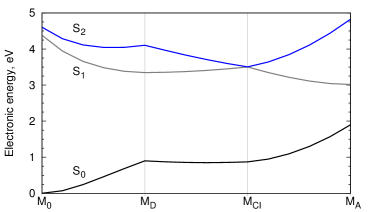
b)

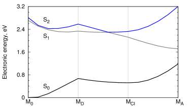
Figure 2: a) Approximate profile at CASSCF/6-31G^∗ level of theory. The curves are obtained by rectilinear interpolations between two consecutive stationary geometries. b) Approximate profile at XMCQDPT2 level of theory. The curves are obtained by rectilinear interpolations between two consecutive stationary geometries obtained at CASSCF/6-31G^∗ level of theory.

We observed an exchange of configuration in the CASSCF electronic states on each side of the CI and the quasi-diabatic states $S_{D}$ and $S_{A}$ (defined in Sec. II.1) are such that: $S_{1}\equiv S_{D}$ and $S_{2}\equiv S_{A}$ at $M_{D}$, while $S_{1}\equiv S_{A}$ and $S_{2}\equiv S_{D}$ at $M_{D}$. This observation supports our approach to building a two-state crossing diabatic model for this ET reaction. The conical intersection seam minimum and adiabatic surfaces around it are plotted along the branching plane modes in Fig. 3. Figure 3 shows a very small splitting along one of the directions. Therefore, the crossing subspace is almost $\mathcal{D}-1$ dimensional, where $\mathcal{D}$ is the total number of nuclear dimensions, which is consistent with small diabatic coupling between the crossing diabats. Fernández et al. (2000); Blancafort et al. (2001)

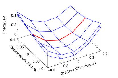
Figure 3: Adiabatic electronic energies in the branching space in the vicinity of the minimum of the CI seam obtained at the CASSCF/6-31G^∗ level. The coordinates’ origin is set at $M_{CI}$. The two directions and their scales are defined by orthonormalizing the covariant gradient difference with respect to the non-adiabatic coupling vector in mass-weighted coordinates. The lower surface is the first excited state, $S_{1}$, while the upper surface is the second excited state, $S_{2}$. The red line indicates a line of quasi-degeneracy between the two states.

A local electronic excitation of the lumiflavin leads to reorganization of the $\pi$ orbital system that exerts a force on the nuclei in the Franck-Condon region (see the gradient of $S_{1}$ energy at $M_{0}$ geometry in Fig. 4-a). Moving from the Franck-Condon region along the gradient modifies bond orders between nuclei in the lumiflavin plane. Therefore, it also changes the hybridization of nitrogens responsible for the bent conformation of lumiflavin from $sp^{3}$ to a $sp^{2}$ and leads to planar lumiflavin in the excited electronic state. The relative coupling between the two directions in the $S_{1}$ Hessian is $2.16$, mis which indeed proves that the force at the Franck-Condon (FC) point will induce a change of the lumiflavin conformation from bent to planar. This analysis agrees with the planar geometry of lumiflavin found at $M_{D}$. Hence, main nuclear coordinates involved in motion from $M_{0}$ to $M_{D}$ are lumiflavin out-of-plane coordinates as can be seen from the corresponding displacement vector given in Fig. 4-c.

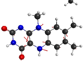
a)		b)
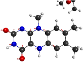
c)		d)
e)		f)

Figure 4: a) Energy gradient vector at $M_{0}$ geometry on the first excited electronic state. b) Derivative coupling for the CI between first and second electronic excited states at $M_{CI}$. c) Displacement vector from geometry $M_{0}$ to $M_{D}$. This vector is mainly the out-of-plane motion of the lumiflavin nuclei. d) Displacement vector from $M_{D}$ to the CI. e) Gradient difference for the CI between first and second electronic excited states at $M_{CI}$. f) Displacement vector from $M_{D}$ to $M_{A}$.

The ET process proceeds from the flavin $\pi^{*}$ system to the $\pi^{*}$ orbital of the CPD carbonyl group. Thus, the carbon of the carbonyl group on CPD changes its hybridization from $sp^{2}$ to $sp^{3}$ and the carbonyl orientation with respect to the thymine ring becomes bent, while changes in the lumiflavin $\pi$ system cause bond reordering. Both motions are described by the branching space vectors given in Figs. 4-b and 4-e.

The FB motion was also found to participate in accessing the $M_{CI}$ from $M_{D}$ or $M_{A}$ as can be seen in Fig. 4-d. However, these displacement vectors have small amplitudes and removing the FB coordinate must not change the $M_{CI}$ position significantly. Reoptimization of the CI seam minimum without including the FB coordinate leads to geometry that is very similar to and only 30 meV higher in energy than that with including the FB coordinate. Stationary point optimizations with constrained FB for the model $N$ gave new geometries that can be found in the supplemental materials. Joubert-Doriol et al. (2015) Only the minimum of the ground state $M_{0}$ is significantly affected while other stationary points were already almost planar without the constraints, and their changes in energy are of only few dozens of meV. The CI seam still shows a $\mathcal{D}-1$ crossing subspace, which implies a very small coupling between the electronic states. However, FB participates in connecting the excited states and the CI seam minima. Therefore, the distances between $M_{CI}$, $M_{D}$, and $M_{A}$ are smaller after removing the FB coordinates.

III.2 ET lifetimes

The five primary modes connect the stationary points ($M_{0}$, $M_{D}$, $M_{A}$, and $M_{CI}$) and describe the two branching space vectors at $M_{CI}$. A grid is built along these five dimensions at the CASSCF level for the fitting procedure. A visual comparison of the errors between the CASSCF/6-31G^∗ calculations and the $B_{pri}$ model along the approximate profile and along the branching space modes at the vicinity of $M_{CI}$ can be found in the supplemental materials. Joubert-Doriol et al. (2015)

Initial conditions for the quantum dynamics are chosen as a Boltzmann distribution in $S_{D}$ at $298$ K. This choice is made assuming that the relaxation of the nuclear subsystem in $S_{D}$ does not affect appreciably the ET process. This assumption is based on approximate orthogonality between the relaxation direction $(M_{0},M_{D})$ and active coordinates of the ET process, which are given by the direction $(M_{D},M_{A})$ and the branching space vectors. Indeed, $(M_{0},M_{D})$ is almost orthogonal to the direction $(M_{D},M_{A})$ with an angle $\widehat{M_{0}M_{D}M_{A}}=76^{\circ}$ (see Figs. 4-a and  4-f) and the two directions are very weakly coupled with a relative coupling of $9.5\cdot 10^{-3}$ in the Hessian. mis Moreover, the direction $(M_{0},M_{D})$ is orthogonal to the branching space (see Figs. 4-b and 4-e) with an angle of $87^{\circ}$ so the crossing region is not easily accessed by the system from $M_{0}$. Long ET time-scale provides the system with enough time to relax on the excited state before the ET process. For a Boltzmann distribution in $S_{D}$ as the initial condition, the correlation function [Eq. (II.3)] depends only on the difference $t^{\prime}-t^{\prime\prime}$. Thus $f(t^{\prime},t^{\prime\prime})=f(0,t^{\prime\prime}-t^{\prime})\equiv f(t^{\prime\prime}-t^{\prime})$ with

$$f(t) = 2\Re\left\langle V_{c}(0)V_{c}(t)\right\rangle_{T}.$$ (9)

With this simplification, the donor population Eq. (6) takes a simpler form

$$P_{D}(t) = e^{\int_{0}^{t}dt^{\prime}f(t^{\prime})t^{\prime}}e^{-t\int_{0}^{t}dt^{\prime}f(t^{\prime})}.$$ (10)

The model $B_{pri}$ shows an exponential decay with a full population transfer (red curve in Fig. 5) due to vibrational state resonances between $S_{D}$ and $S_{A}$. Endicott, Joubert-Doriol, and Izmaylov (2014) The theoretical lifetime is $10$ ps, which has to be compared with the experimental one of $170$ ps. Kao et al. (2005) Given the simplified assumptions used to construct our model, we consider this to be in qualitative agreement. The long time scale indicates that the $B_{pri}$ model correctly accounts for the small coupling between the electronic states. The energies from single points calculation at the XMCQDPT2 level of theory given in Fig. 2-b are used to adjust the diabatic elements of the model $B_{pri}$. As expected from the displacement of the CI seam minimum, after adding the XMCQDPT2 corrections, the lifetime becomes shorter, $2$ ps.

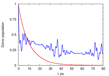
Figure 5: Time evolution of the $S_{D}$ population for the primary system model including ($B_{pri}$ in red) or not ($N_{pri}$ in blue) the lumiflavin butterfly motion. Vibronic resonances in $B_{pri}$ induce a full population transfer while the absence of such resonances in $N_{pri}$ causes oscillations.

III.3 Variations of the primary system model

The lifetime is sensitive to parameter variations in quadratic terms. These terms can be separated in three groups: 1) quadratic terms in $V_{c}$ (diabatic coupling) contained in the matrix $K_{c,\alpha\beta}$ used in Eq. (2); 2) contributing to differences between the donor and acceptor state normal mode frequencies $\{\Omega_{D,\alpha}\}$ and $\{\Omega_{A,\alpha}\}$; 3) contributing to Duschinsky rotation, a transformation $\{R_{\alpha\beta}\}$ to obtain the acceptor state normal modes $Q_{A,\alpha}=\sum_{\beta}R_{\alpha\beta}Q_{D,\beta}$ from the donor state normal modes $\{Q_{D,\alpha}\}$. The last two groups can be linked to coefficients $K_{D,\alpha\beta}$ and $K_{A,\alpha\beta}$ used in Eq. (2):

$$\sum_{\alpha,\beta}x_{\alpha}K_{D,\alpha\beta}x_{\beta} = \sum_{\alpha}\frac{1}{2}\Omega_{D,\alpha}^{2}Q_{D,\alpha}^{2},$$

$$\sum_{\alpha,\beta}x_{\alpha}K_{A,\alpha\beta}x_{\beta} = \sum_{\alpha}\frac{1}{2}\Omega_{A,\alpha}^{2}Q_{A,\alpha}^{2}$$ (11)

$$= \sum_{\alpha}\frac{1}{2}\Omega_{A,\alpha}^{2}\Big{[}\sum_{\beta}R_{\alpha\beta}Q_{D,\beta}\Big{]}^{2},$$

and it can be noticed that $\bm{K}_{A}=\bm{K}_{D}$ if $\bm{\Omega}_{A}=\bm{\Omega}_{D}$ and $\bm{R}=\bm{1}$. To see effects of these terms on lifetimes we contrasted the results for full QVC models with those obtained omitting each group of terms separately (see Table 1). The model’s variations modify the lifetime such that the ET process can be blocked (a lifetime larger by more than four orders of magnitude), which shows the importance of the quadratic terms in the model.

model	QVC	$\bm{K}_{c}$=0	$\bm{R}=\bm{1}$	$\bm{\Omega}_{A}=\bm{\Omega}_{D}$
$B_{pri}$	$10$	$10$	$11$	NT
$B_{ful}$	$1$	$2$	NT	NT
$N_{ful}$	$0.3$	$0.5$	NT	$4$

Table 1: Lifetimes given in picoseconds for different variations of the diabatic models including. NT: no transfer happens with an estimate of the lifetime larger than 0.1 $\mu$sec ($\tau>10^{5}$).

Removing the quadratic terms in $V_{c}$ ($\bm{K}_{c}=0$) does not affect strongly the lifetime, which can be understood because the coupling between the two states is already very small. In contrast, imposing the same quadratic terms in both states results in much longer lifetimes. After decomposing $\bm{K}_{D}-\bm{K}_{A}$ in terms of Duschinsky rotation and frequency differences, it is easy to realize from Table 1 that imposing the same vibrational frequencies for both diabatic states changes lifetimes drastically by modifying resonances between the two electronic states.

III.4 Full dimensional models

Adding residual modes makes the correlation functions Eq. (9) decay within few tens of femtoseconds (see Fig. 6).

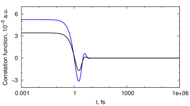
Figure 6: Correlation function in logarithmic time axis for the various full-dimensional models. Blue lines are for models that include the FB, while black lines does not.

Defining $t_{0}$ as the decay time in which the correlation function, $f(t)$, becomes numerical 0. For both models with residual modes $t_{0}\approx 20$ fs, hence $t_{0}\ll\tau_{D}$ (ps) and we can make a Markovian approximation for the donor population given by Eq. (10)

$$P_{D}(t) \approx e^{\int_{0}^{t_{0}}dt^{\prime}f(t^{\prime})t^{\prime}}e^{-t\int_{0}^{t_{0}}dt^{\prime}f(t^{\prime})}.$$ (12)

According to Eq. (8) and Eq. (12) the donor state lifetime $\tau_{D}$ is defined as

$$\tau_{D} = \left[\int_{0}^{t_{0}}dt^{\prime}f(t^{\prime})\right]^{-1}.$$ (13)

Including additional modes generally increases the reorganization energy, and according to the Marcus theory is expected to slow down the ET process. In contrast, in our simulations, adding the secondary modes decrease the lifetime (see $B_{ful}$ in Table 1). To understand this effect, one has to remember that the additional modes also contribute to the coupling term, $V_{c}$. Even if the individual contributions to the linear coupling vector $\bm{v}_{c}$ (Eq. (II.2)) from each secondary mode is small, owing to the overall large number of these modes, their total contribution is of the same order of magnitude as the contribution from the primary system. Their effect can be estimated by looking at the ratio of the coupling vector norm, $||\bm{v}_{c}||$, over the norm of the difference of the linear term for diabatic energies, $||\bm{v}_{A}-\bm{v}_{D}||$, the latter is associated with the reorganization energy. For $B_{pri}$ this ratio is $0.3$, while for $B_{ful}$ it is $0.9$. The inclusion of secondary modes emphasizes the importance of the Duschinsky rotation as can be seen in Table 1. Therefore, it is crucial for adequate modelling of $B_{ful}$ to account for different orientations of normal modes in the two electronic states.

III.5 Role of the FB motion

The procedure to obtain the parameters for the model $N_{pri}$ is the same as for the model $B_{pri}$ except that the FB motion is constrained for geometry optimizations as described in Sec.II.1 and the new stationary points are used in the fitting procedure. The same number of stationary points are obtained for $N_{pri}$ as for $B_{pri}$. Hence, both models are 5D. Population dynamics in these models (Fig. 5) show that the FB motion has a strong impact on the dynamics. In contrast to the dynamics in $B_{pri}$, the $N_{pri}$ dynamics does not show a full transfer but rather has population oscillations. Moreover, the latter dynamics starts with a fast initial drop within the first hundred femtoseconds followed by oscillations. The oscillations appearing for the $N_{pri}$ model indicate that the vibrational states of the donor and acceptor wells are not in resonance. Including the low frequency FB mode in the $B_{pri}$ model increases the density of vibrational states and induces resonances, which remove population oscillations and lead to a complete population transfer. Thus, one role of the FB motion is to induce decoherence. Because of the oscillations in $N_{pri}$, no lifetime can be extracted in this case. Adding the secondary modes causes decoherence and complete ET. Therefore, we can calculate the lifetime for $N_{ful}$ and compare it with the lifetime obtained in $B_{ful}$. The FB motion slows down the ET by almost one order of magnitude in full-dimensional models (see $N_{ful}$ compared to $B_{ful}$ in Table 1). The slower ET in $B_{ful}$ does not happen because of a smaller coupling ($||\bm{v}_{c}||$ is of the same magnitude for $B_{pri}$ and $N_{pri}$), it is rather due to smaller Franck-Condon factors appearing from the Duschinsky rotation terms as can be seen in Table 1. Therefore, another role of the FB motion is to decrease Franck-Condon factors.

IV Conclusion

Above, we present the first diabatic PES models for the ET process that initiates the CPD lesion repair in the CPD-photolyase complex. Our models give lifetimes between one (for the $109$-dimensional model) and ten picoseconds (for the $5$-dimensional model), which is one order of magnitude faster (but still relatively close if compared with other ultrafast processes) than the ET timescale measured experimentally (170 ps). Slow rates of ET in our models is attributed to small diabatic coupling between the two diabatic electronic states, and even if the crossing region between electronic states is easily accessible, the system remains diabatically trapped. We showed that the quadratic terms used in the expansions of the diagonal elements of our diabatic model (frequency differences and Duschinsky rotation of normal modes) must be included as they are essential for modelling Franck-Condon factors which regulate the ET process. In contrast, the quadratic terms in the off diagonal diabatic couplings are negligible. Investigation concerning the inclusion or exclusion of the FB coordinate showed the importance of this mode for dynamics as it enhances incoherent transfer by increasing density of vibrational states due to its low vibrational frequency. The intrinsic properties of the donor-acceptor complex at the geometry controlled by binding to the protein are favorable for ET without a “mediator” as proposed for adenine. Liu et al. (2012) However, adenine might be involved in “adjusting” the donor and acceptor energies in the protein DNA complex (as opposed to the considered here CPD-flavin complex), where for instance, negative phosphates in the proximity of donor and acceptor may alter the state energies. Moughal Shahi and Domratcheva (2013)

In future work we will focus on the effects of amino acid residues present in the active site and will assess the importance of the protein environment in order to obtain quantitative estimations of the lifetime. A simple method we developed in this paper can be also applied to other steps of the CPD repair process, in particular the electron back transfer. It can also be applied to the pyrimidine-pyrimidone (6-4) photoproduct repair process and give insights on the futile electron back transfer Li et al. (2010) by comparison with the CPD process. Models generated in this paper can be further used to study the effect of exciting the system with incoherent sunlight Tscherbul and Brumer (2014); Joubert-Doriol and Izmaylov (2015) rather than coherent laser light used in transient spectroscopy experiments. Kao et al. (2005)

V Aknowledgments

LJD thanks Dvira Segal for providing some computational resources and the European Union Seventh Framework Programme (FP7/2007-2013) for financial support under grant agreement PIOF-GA-2012-332233. TD acknowledges support through the Minerva program of the Max Planck Society.

Appendix A Diabatic potential parametrization

The Hessians of the diabatic states, $\bm{K}_{D}$ and $\bm{K}_{A}$, in Eq. (2) must be real symmetric positive definite matrices. Hence, we naturally choose to parameterize $\bm{K}_{D}$ and $\bm{K}_{A}$ using the Cholesky decomposition

$$\bm{K}_{k} = \bm{L}_{k}^{T}\bm{L}_{k},$$ (14)

where $\bm{L}_{k}$ is a lower triangular matrix. Any global unitary transformation

$$\bm{U}(\theta,\phi,\psi) = \big{(}\begin{smallmatrix}e^{\dot{\imath}\phi}&0\\ 0&e^{-\dot{\imath}\phi}\end{smallmatrix}\big{)}\big{(}\begin{smallmatrix}\cos\theta&-\sin\theta\\ \sin\theta&\phantom{-}\cos\theta\end{smallmatrix}\big{)}\big{(}\begin{smallmatrix}e^{\dot{\imath}\psi}&0\\ 0&e^{-\dot{\imath}\psi}\end{smallmatrix}\big{)}$$ (15)

of the diabatic potential [$\bm{V}=(\begin{smallmatrix}V_{D}&V_{c}\\ V_{c}&V_{A}\end{smallmatrix})$, Eq. (2)] leads to a different diabatic model $\tilde{\bm{V}}=\bm{U}^{\dagger}\bm{V}\bm{U}$, which gives back the same adiabatic energies and the same quantum dynamics.

Since the diabatic state potentials must be bounded in any representation, the Hessians of the diabatic states must be positive definite for any value of $\phi$, $\theta$, and $\psi$. This positivity imposes some constraints on possible values of $K_{c}$ elements. All possible Hessians generated by the transformation can be written as

$$\bm{K}_{\theta} = (\bm{K}_{A}+\bm{K}_{D})+\cos(2\theta)(\bm{K}_{A}-\bm{K}_{D})$$ (16)

$$\hskip 55.48277pt+2\cos(\phi)\sin(2\theta)\bm{K}_{c},$$

where $\theta$ and $\phi$ are parameters of the unitary transformation of the diabatic states. A parametrization of $\bm{K}_{c}$ that ensures the positivity of the Hessian given in Eq. (16) is still an open problem. Horn (1962); Fulton (2000) We can fix $\phi$ to $0$ because it does not affect $K_{c}$ parametrization. Indeed, if for a given $\theta$ $\bm{K}_{\theta}$ is positive for $\cos(\phi)=\pm 1$, then it is also positive for $-1<\cos(\phi)<1$ because the highest absolute eigenvalue of the matrix $\cos(\phi)\bm{K}_{c}$ can only be smaller. The Cholesky decompositions of $\bm{K}_{D}$ and $\bm{K}_{A}$ already impose positivity for the cases $\theta=0,\pi/2$. Positivity for $\theta=\pm\pi/4$ ($\bm{K}_{\theta}=\bm{K}_{A}+\bm{K}_{D}\pm 2\bm{K}_{c}$) can be ensured by using the following parametrization Au-Yeung (1969)

$$\bm{K}_{c} = \frac{1}{2}\bm{L}_{s}^{T}e^{-\bm{A}}\operatorname{diag}(atan(\bm{r}))e^{\bm{A}}\bm{L}_{s},$$ (17)

where $\bm{L}_{s}$ is the Cholesky decomposition of $\bm{K}_{A}+\bm{K}_{D}$, $\bm{A}$ is a real anti-symmetric matrix, and $\bm{r}$ is a real-valued vector.

The parametrization given in Eq. (17) is used in the primary modes parameter optimization. However, for optimizations of the full-dimensional models this parametrization becomes more difficult to implement and cannot be combined with constraints unless we substitute the steepest descent algorithm for another more computationally expensive one. To avoid this extra computational cost, we change the parametrization of $\bm{K}_{c}$ for this latter case to ensure positivity when $\theta=\pi/4$ ($\bm{K}_{\theta}=\bm{K}_{A}+\bm{K}_{D}+2\bm{K}_{c}$):

$$\bm{K}_{c} = \frac{1}{2}\left(\bm{L}_{c}^{T}\bm{L}_{c}-\bm{K}_{A}-\bm{K}_{D}\right),$$ (18)

where the matrix $\bm{L}_{c}$ represents a set of parameters to be optimized for changing $\bm{K}_{c}$.

There are values of $\theta$ for which the positivity of $\bm{K}_{\theta}$ cannot be ensured by the parametrization. In these cases, we build a grid in the range $]-\pi/2:\pi/2]$ on which we check the positivity of $\bm{K}_{\theta}$.

Appendix B Optimization of the full-dimensional model’s parameters

Here we describe our method of obtaining the parameters for the full-dimensional QVC models. The idea is based on the following expression for adiabatic energies of a two-electronic state system

$$E_{\pm} = (\Sigma\pm\Omega)/2$$ (19)

where $E_{\pm}$ are the adiabatic energies for lower, $S_{1}$, and upper, $S_{2}$, electronic states, $\Sigma$ is the sum of adiabatic energy, $\Omega$ is the absolute adiabatic energy difference. $\Omega$ is non-linear with respect to the diabatic elements given by

$$\Omega^{2} = \Delta^{2}+4V_{c}^{2}$$ (20)

where $\Delta=V_{A}-V_{D}$ is the diabatic energy difference and $V_{c}$ is the diabatic coupling between diabatic electronic states [see Eq. (2)]. Equation (19) suggests to fit the sum and the energy difference separately such that the sum part (quantities $\bm{\nabla}\Sigma$, $\bm{\nabla}\bm{\nabla}^{T}\Sigma$ at $M_{0}$, $M_{D}$ and $M_{A}$) can be fitted linearly to obtain full dimensional $\bm{v}_{D}+\bm{v}_{A}$, and $\bm{K}_{D}+\bm{K}_{A}$. Because Eq. (20) is non-linear, one can employ a non-linear fitting procedure to obtain diabatic parameters. However, it is possible to avoid this difficulty after inspecting differential forms of Eq. (20) with respect to nuclear coordinates

$$\Omega\bm{\nabla}\Omega = \Delta\bm{\nabla}\Delta+4V_{c}\bm{\nabla}V_{c},$$ (21)

$$(\bm{\nabla}\Omega)(\bm{\nabla}\Omega)^{T}+\Omega\bm{\nabla}\bm{\nabla}^{T}\Omega = (\bm{\nabla}\Delta)(\bm{\nabla}\Delta)^{T}$$

$$+\Delta\bm{\nabla}\bm{\nabla}^{T}\Delta+4(\bm{\nabla}V_{c})(\bm{\nabla}V_{c})^{T}+4V_{c}\bm{\nabla}\bm{\nabla}^{T}V_{c}.$$

Because $M_{0}$, $M_{D}$ and $M_{A}$ are already described by the 5D model, $\Delta$ and $V_{c}$ and especially the quantities $\{\bm{v}_{k}^{T}\bm{x}_{j},\bm{x}_{i}^{T}\bm{K}_{k}\bm{x}_{j};k=D,A,c\}$, where $\bm{x}_{i}$ and $\bm{x}_{j}$ are already known at the coordinate vectors for nuclear configurations $i,j=M_{0},M_{D},M_{A}$. Knowing $\Delta$ and $V_{c}$ at the minima makes possible to turn Eq. (21) and Eq. (B) at the stationary geometries in a set of linear equations with respect to the parameters $\{\bm{v}_{k}\}$ and $\{\bm{K}_{k}\}$. The system of linear equations is generated in two steps: First, we project Eq. (B) on the stationary geometries and combine the resulting equations with Eq. (21). The resulting system of equations can be easily solved as a least square problem to obtain the following linear terms: $\{\bm{v}_{k},\bm{K}_{k}\bm{x}_{j};k=D,A,c;j=M_{0},M_{D},M_{A}\}$. Second, we obtain the quadratic terms of the model by substituting linear terms in Eq. (B), which becomes linear with respect to matrices $\{\bm{K}_{k}\}$.

The special parametrization of the matrices $\{\bm{K}_{k}\}$ given by Eqs. (14) and (18) makes a set of equations for $\{\bm{K}_{k}\}$ non-linear. Therefore, we minimize the corresponding least square problem with the steepest descent algorithm, which requires algebraic manipulations with matrices of only the $\bm{K}_{k}$ size, and thus, is feasible and fast. The minimization is constrained to ensure that we recover the accurate 5D models after projecting the full-dimensional models on the primary modes.

References

- Sancar (2003) A. Sancar, Chem. Rev. 103, 2203 (2003).
- Sancar (2008) A. Sancar, J. Biol. Chem. 283, 32153 (2008).
- Müller and Carell (2009) M. Müller and T. Carell, Curr. Opin. Struct. Biol. 19, 277 (2009).
- Berardesca et al. (2012) E. Berardesca, M. Bertona, K. Altabas, V. Altabas, and E. Emanuele, Mol. Med. Rep. 5, 570 (2012).
- Emanuele et al. (2013) E. Emanuele, V. Altabas, K. Altabas, and E. Berardesca, J. Drugs Dermatol. 12, 1017 (2013).
- Emanuele, Spencer, and Braun (2014) E. Emanuele, J. Spencer, and M. Braun, J. Drugs dermatol. 13, 309 (2014).
- Mees et al. (2004) A. Mees, T. Klar, P. Gnau, U. Hennecke, A. P. M. Eker, T. Carell, and L.-O. Essen, Science 306, 1789 (2004).
- Kao et al. (2005) Y.-T. Kao, C. Saxena, L. Wang, A. Sancar, and D. Zhong, Proc. Natl. Acad. Sci. U.S.A. 102, 16128 (2005).
- Weber (2005) S. Weber, Biochim. Biophys. Acta Functional Redox Radicals in Proteins, 1707, 1 (2005).
- Essen and Klar (2006) L. O. Essen and T. Klar, Cell. Mol. Life Sci. 63, 1266 (2006).
- Zheng, Garcia, and Stuchebrukhov (2008) X. Zheng, J. Garcia, and A. A. Stuchebrukhov, J. Phys. Chem. B 112, 8724 (2008).
- Liu et al. (2012) Z. Liu, X. Guo, C. Tan, J. Li, Y.-T. Kao, L. Wang, A. Sancar, and D. Zhong, J. Am. Chem. Soc. 134, 8104 (2012).
- Antony, Medvedev, and Stuchebrukhov (2000) J. Antony, D. M. Medvedev, and A. A. Stuchebrukhov, J. Am. Chem. Soc. 122, 1057 (2000).
- Blancafort et al. (2001) L. Blancafort, F. Jolibois, M. Olivucci, and M. A. Robb, J. Am. Chem. Soc. 123, 722 (2001).
- Blancafort, Hunt, and Robb (2005) L. Blancafort, P. Hunt, and M. A. Robb, J. Am. Chem. Soc. 127, 3391 (2005).
- Joubert-Doriol, Ryabinkin, and Izmaylov (2013) L. Joubert-Doriol, I. G. Ryabinkin, and A. F. Izmaylov, J. Chem. Phys. 139, 234103 (2013), arXiv:1310.2929 .
- Borrelli and Peluso (2011) R. Borrelli and A. Peluso, Phys. Chem. Chem. Phys. 13, 4420 (2011).
- Borrelli and Peluso (2015) R. Borrelli and A. Peluso, J. Chem. Theo. Comp. 11, 415 (2015).
- Izmaylov et al. (2011) A. F. Izmaylov, D. Mendive-Tapia, M. J. Bearpark, M. A. Robb, J. C. Tully, and M. J. Frisch, J. Chem. Phys. 135, 234106 (2011).
- Endicott, Joubert-Doriol, and Izmaylov (2014) J. S. Endicott, L. Joubert-Doriol, and A. F. Izmaylov, J. Chem. Phys. 141, 034104 (2014).
- Liu et al. (2013) Z. Liu, M. Zhang, X. Guo, C. Tan, J. Li, L. Wang, A. Sancar, and D. Zhong, PNAS 110, 12972 (2013).
- Cederbaum, Köppel, and Domcke (1981) L. S. Cederbaum, H. Köppel, and W. Domcke, Int. J. Quantum Chem. 20, 251 (1981).
- Köppel, Domcke, and Cederbaum (1984) H. Köppel, W. Domcke, and L. S. Cederbaum, “Multimode Molecular Dynamics Beyond the Born-Oppenheimer Approximation,” (John Wiley & Sons, Inc., 1984) Chap. 2, pp. 59–246.
- Joubert-Doriol et al. (2014) L. Joubert-Doriol, B. Lasorne, D. Lauvergnat, H.-D. Meyer, and F. Fabien Gatti, J. Chem. Phys. 140, 044301 (2014).
- Domratcheva (2011) T. Domratcheva, J. Am. Chem. Soc. 133, 18172 (2011).
- Walsh and Miller (2003) J. D. Walsh and A.-F. Miller, J. Mol. Struct.: THEOCHEM 623, 185 (2003).
- Kao et al. (2008) Y.-T. Kao, C. Saxena, T.-F. He, L. Guo, L. Wang, A. Sancar, and D. Zhong, J. Am. Chem. Soc. 130, 13132 (2008).
- Joubert-Doriol et al. (2015) L. Joubert-Doriol, T. Domratcheva, M. Olivucci, and A. F. Izmaylov, “Supplemental material,” (2015).
- Udvarhelyi and Domratcheva (2011) A. Udvarhelyi and T. Domratcheva, Photochem. Photobiol. 87, 554 (2011).
- Granovsky (2011) A. A. Granovsky, J. Chem. Phys. 134, 214113 (2011).
- Granovsky (2015) A. A. Granovsky, J. Chem. Phys. 143, 231101 (2015).
- (32) A. A. Granovsky, “Firefly version 8.0,” .
- Schmidt et al. (1993) M. Schmidt, K. Baldridge, J. Boatz, S. Elbert, M. Gordon, J. Jensen, S. Koseki, N. Matsunaga, K. Nguyen, S. Su, T. Windus, M. Dupuis, and J. Montgomery, J.Comput.Chem. , 1347 (1993).
- Köppel, Yarkony, and Barentzen (2010) H. Köppel, D. R. Yarkony, and H. Barentzen, eds., The Jahn-Teller Effect, Springer Series in Chemical Physics, Vol. 97 (Springer Berlin Heidelberg, Berlin, Heidelberg, 2010).
- Levenberg (1944) K. Levenberg, Q. Appl. Math. 2, 164 (1944).
- Marquardt (1963) D. W. Marquardt, J. Soc. Ind. Appl. Math. 11, 431 (1963).
- Nelder and Mead (1965) J. A. Nelder and R. Mead, Comp. J. 7, 308 (1965).
- Mat (2012) “Matlab, version 8.0.0.783 (r2012b),” The MathWorks Inc., Natick, Massachusetts (2012).
- Fernández et al. (2000) E. Fernández, L. Blancafort, M. Olivucci, and M. A. Robb, J. Am. Chem. Soc. 122, 7528 (2000).
- (40) “The relative coupling between the two directions and is given by , where is the element of the adiabatic hessian matrix in the electronic state.” .
- Moughal Shahi and Domratcheva (2013) A. R. Moughal Shahi and T. Domratcheva, J. Chem. Theory Comput. 9, 4644 (2013).
- Li et al. (2010) J. Li, Z. Liu, C. Tan, X. Guo, L. Wang, A. Sancar, and D. Zhong, Nature 466, 887 (2010).
- Tscherbul and Brumer (2014) T. V. Tscherbul and P. Brumer, J. Phys. Chem. A 118, 3100 (2014).
- Joubert-Doriol and Izmaylov (2015) L. Joubert-Doriol and A. F. Izmaylov, J. Chem. Phys. 142, 134107 (2015).
- Horn (1962) A. Horn, Pacific J. Math. 12, 225 (1962).
- Fulton (2000) W. Fulton, Bull. Amer. Math. Soc. 37, 209 (2000).
- Au-Yeung (1969) Y.-H. Au-Yeung, Proc. Am. Math. Soc. 20, 545 (1969).