Electromagnetic gauge-freedom and work
Abstract
We argue that the definition of the thermodynamic work done on a charged particle by a time-dependent electromagnetic field is an open problem, because the particle’s Hamiltonian is not gauge-invariant. The solution of this problem demands accounting for the source of the field. Hence we focus on the work done by a heavy body (source) on a lighter particle when the interaction between them is electromagnetic and relativistic. The work can be defined via the gauge-invariant kinetic energy of the source. We uncover a formulation of the first law (or the generalized work-energy theorem) which is derived from relativistic dynamics, has definite validity conditions, and relates the work to the particle’s Hamiltonian in the Lorenz gauge. Thereby the thermodynamic work also relates to the mechanic work done by the Lorentz force acting on the source. The formulation of the first law is based on a specific separation of the overall energy into those of the source, particle and electromagnetic field. This separation is deduced from a consistent energy-momentum tensor. Hence it holds relativistic covariance and causality.
pacs:
05.70.Ln, 13.40.-f, 45.20.dhI Introduction
Equilibrium statistical thermodynamics is based on notions of work, heat, entropy and temperature balian ; lindblad ; mahler . The primary concept of non-equilibrium statistical mechanics is work, because its definition is relatively straightforward balian ; lindblad ; mahler . This is witnessed by recent activity in non-equilibrium (classical and quantum) physics that revolves around the work and the laws of thermodynamics lindblad ; mahler ; lehrman ; mukamel ; jarb ; leff ; campisi ; skr ; armen ; gallego ; aspects ; plastina ; 3law ; rubi ; peliti ; silbey ; rubirubi ; jar .
We recall the definition of the thermodynamic work and its features. Consider a non-relativistic particle with coordinate , canonic momentum and Hamiltonian , where is an external field. The thermodynamic work done on the particle by the field’s source in the time-interval is balian ; lindblad ; mahler :
| (1) |
equals the energy increase of the particle. No work is done if is time-independent. Definition (1) generalizes to statistical situations, where the description goes via probability densities or via density matrices balian ; lindblad ; mahler . It appears in the laws of thermodynamics.
There is an alternative definition of the thermodynamic work balian ; lindblad ; mahler
| (2) |
It applies to the open-system situation, e.g. particles interacting with baths balian ; lindblad ; mahler . Eq. (2) leads to (1) due to the Hamilton equations of motion.
If is a coordinate of the source, the full time-independent Hamiltonian of the system and source reads111Even if is not a coordinate, (1, 2) stay consistent as far as the system and the work-source form a closed system.
| (3) |
where is the momentum of the source, and is its Hamiltonian. The time-dependent Hamiltonian of the system in (1, 2) results from (3), if the reaction of the system to the source is neglected, e.g. because the source is heavy.
Two important features of the thermodynamic work (1) are displayed via (2, 3). First, since the total energy (3) is conserved, the thermodynamic work (1) relates to the energy change of the source balian ; lindblad ; mahler . Second, (2, 3) show that is the potential force acting (from the particle) to the source. Then (2) relates to the mechanic concept of work: force times the displacement leff .
Let now the external field be electromagnetic (EMF). The relativistic Hamiltonian of a particle reads landau ; kos
| (4) | |||
| (5) |
where is the 4-potential of EMF, () is the kinetic (canonic) momentum, , and are the coordinate, mass and charge, respectively. For a non-relativistic particle, is replaced by .
The thermodynamic work cannot be read directly from (1, 2, 4), because neither nor its time-difference stay invariant under a gauge-transformation defined via a function ) yang ; kobe ; zambrano ; lorce_review ; grif :
| (7) | |||||
The kinetic momentum in (4) is gauge-invariant. But is not yang ; kobe 222 This differs from a formally similar gauge-freedom issue that appears even for the non-relativistic situation (1) rubi ; peliti ; silbey ; rubirubi . This issue is resolved easily by choosing as e.g. the coordinate of a physical source of work rubi ; peliti ; silbey ; rubirubi ; jar ; see (3) and Appendix A. . The same problem exists for a quantum particle interacting with EMF yang ; kobe .
One response to the EMF gauge-freedom problem is that the gauge in (4) is to be selected as (temporal gauge) landau ; kos ; kobe :
| (8) |
This definition is indirectly supported by the standard EMF energy-momentum tensor, which suggests that particles do not have potential energy landau ; kos ; see Appendix B. Eq. (4) under implies that the sought thermodynamic work would amount to the particle’s kinetic energy change, i.e. to the mechanic work done on the particle by the Lorentz force landau . This cannot be the correct definition of the thermodynamic work. First, because it implies that time-independent fields do thermodynamic work reiss_1 ; reiss_2 333Consider a constant electric field . The temporal gauge is achieved by taking in (7), which brings in a time-dependent and shows from (1, 4) that the work done is not zero and equals to the change of the kinetic energy. The latter is non-zero, since only is conserved in time landau .. Second, because this work (2) relates to the force acting on the source, and not to the force acting on the particle.
Another possibility for resolving the gauge-freedom is to employ in (4) the Coulomb gauge sipe ; wang_pra :
| (9) |
But the scalar potential in the gauge (9) propagates with infinite speed stewart ; heras_coulomb ; wundt 444The Maxwell equation reads landau : . Upon using (9) we get for time-dependent in the Coulomb gauge the “static” equation implying that responds instantly to changes in the charge density stewart ; heras_coulomb ; wundt . While this is consistent with electric and magnetic fields propagating with speed stewart ; heras_coulomb ; wundt , it also means that —and the Hamiltonian (4) defined via it—cannot be given a direct physical meaning.
For both proposals it is unclear how the work defined via (4) relates to the energy of the source (heavy body).
Noting the difficulties with the temporal and Coulomb gauge, it is natural to look at the Lorenz gauge,
| (10) |
which is relavistic invariant and causal, i.e. and defined from (10) propogate with speed heras_lorenz ; dmitro . Given (10) and standard boundary conditions of decaying at spatial infinity, is uniquely expressed via gauge-invariant electromagnetic field , and hence it is observable heras_lorenz . If the photon is found to have a small (but finite) mass, (10) will hold automatically massphoton . These features are suggestive, but they do not suffice for defining the thermodynamic work.
Our results validate the usage of (4, 10), and also show that main features of the thermodynamic work generalize to the relativistic, electromagnetic situation:
– The definition of the (thermodynamic) work based on (4, 10) results from a separation of overall (source + particle(s) + EMF) energy into specific components. This separation is not arbitrary, but emerges from a relativistically covariant energy-momentum tensor for the overall system; see section II. necessarily differs from the standard energy-momentum tensor (e.g. because has to account for a potential energy), but it leads to the same values of the overall energy. It consistently relates to an angular momentum (tensor). Certain aspects of are known from puthoff ; bogo , but in its entirety it is proposed for the first time 555Energy-momentum tensors are not uniquely defined, and different situations may require different definitions. An example of this is the dielectric media (not considered here), where different experiments demand different forms of this tensor grif ..
– The approach leads to a formulation of the first law for a relativistic thermally isolated situation, which we demonstrate for point charges with retarded electromagnetic interactions. According to this formulation, the thermodynamic work can be defined through the gauge-invariant kinetic energy of the source, but it is also equal to the change of (4) in the Lorenz gauge. As compared to the non-relativistic first law—which is an automatic consequence of energy conservation lindblad ; balian ; mahler ; lehrman ; leff [cf. (3)]—the formulation is necessarily approximate, since some energy is stored in the (near) EMF, even if the radiated energy is negligible. Once the thermodynamic work amounts to the kinetic energy of the source, it directly relates it to the mechanic work done by the Lorentz force acting on the source. Thus the two important features (described after (3)) generailze to the relativistic, electromagnetic situation.
Several recent studies looked at the work done by EMF in the context of fluctuation theorems deffner ; uribe ; saha ; pradhan ; yet_another . But the problem of the EMF gauge-freedom was not addressed, partially due to implicitly assumed magnetostatic limit, where the gauge (9) is employed by default, and where (10) and (9) are approximately equal lar ; rouss_epl .
This paper is organized as follows. Section II derives from equations of motion a new expression for the energy-momentum tensor of EMF. Appendix B compares with the standard approach to this tensor. Section III recalls the relativistic dynamics of two point charges. This framework serves for formulating the first law in section IV. Sections V shows that the formulation extends to certain situations, where the radiation reaction is essential. The last section summarizes and outlines open problems.
We use Gaussian units and metric . Vectors are denoted as and . We denote and for the 4-coordinate and 4-gradient, respectively.
II Equations of motion and energy-momentum tensor
Consider electromagnetic field (EMF) coupled with a charged continuous matter with mass denisty , charge density and 4-velocity
| (11) |
The comoving frame mass density and charge density read, respectively (omitting ):
| (12) |
Dealing with a continuous matter allows us to postpone the treatment of infinities related to point particles.
The mass and charge conservation read, respectively
| (13) |
where is the charge current. Equations of motion for matter+EMF in the gauge (10) read landau ; kos 666Eqs. (14, 15) are normally obtained via (10). But one can employ (14) and (13) for deriving the Lorenz gauge (10) oost ; fock ; gritsunov . :
| (14) | |||
| (15) |
where , and is the proper time.
The energy-momentum of matter reads landau
| (16) |
where the pressure has been neglected. Eq. (15) implies
| (17) |
We now deduce a conserved energy-momentum tensor from (13–17). Guided by the analogy with a free scalar, massless field whose energy-momentum tensor is bogo , we suggest
| (18) | |||
| (19) |
where (19) is the energy-momentum tensor of the free EMF, is given by (16), and in (18) is due to the interaction. Eqs. (13–17) lead to 4 conservation laws
| (20) |
Eqs. (20, 18) imply that is the energy density
| (21) | |||||
| (22) |
Eq. (21) is the energy density of EMF, while (22) amounts to the energy of the matter that consists of kinetic and the interaction term. The latter will be shown to be the particle’s potential energy in section IV. The possibility of this interpretation is confirmed by the form of energy current:
| (23) | |||||
| (24) |
where (23) is the energy current of EMF.
Eq. (19) for the free EMF was previously derived from the Fermi’s Lagrangian fermi ; bogo ; oost ; see Appendix C. Eqs. (21–24) were discussed in puthoff as alternatives to standard expressions (i.e. the Poynting vector), but were not derived from a consistent energy-momentum tensor. Various proposals for the energy flow of (free) EMF are given in slepian . Their general drawback is that they do not start from a consistent energy-momentum tensor.
All above expressions—including —that contain (in the Lorenz gauge (10)) are gauge-invariant, because can be expressed via heras_lorenz :
| (25) | |||
| (26) | |||
| (27) |
where is the retarded Green’s function, , , is the step function, and is the Dirac’s delta-function. Eq. (25) relates to the retarded solution of (14). Its derivation from (26) is straightforward, e.g. by employing (10) in and integrating by parts.
The main reason for introducing is to verify that the potential energy can emerge from a consistent energy-momentum tensor; the standard energy-momentum tensor of EMF does not allow such an interpretation; see Appendix B. Without a potential energy we cannot define the thermodynamic work via (1, 2); cf. the discussion around (8).
Both (18) and the standard tensor lead to the same expressions for energy (and momentum) of the matter+EMF [see Appendix D]:
| (28) |
where the integration over the full 3-space is taken (assuming that all fields nullify at infinity), is the Larmor’s electromagnetic enegy density expressed via the electromagnetic field (it follows the standard energy-momentum tensor landau ), and is the kinetic energy density for the matter; see (16, 12). The same enters also ; cf. (21, 22). Thus whenever only the total energy matters, agrees with the standard predictions (28). However, generally the density is not equal to given by (19). Differences and similarities between (18) and the standard energy-momentum tensor of EMF are discussed in Appendices B and D; e.g. for spherical waves (19) produces the same expression as the standard tensor.
Note that the free EMF tensor (19) is symmetric, , as it should, because this ensures the known relation between the energy current and the momentum density ; cf. (23). But the full tensor (18) is not symmetric, , due to the EMF-matter coupling. Appendix E discusses the meaning of this asymmetry and relates to the angular momentum and spin tensor. These relations are necessary to establish, because the angular momentum is employed for explaining the energy of EMF feynman ; slepian ; pugh .
III Two point-particles without self-interactions
For two point particles and we take in (12–15):
| (29) | |||
| (30) |
where , and are the trajectory, charge and mass of (resp. for ), and where is the delta-function. It is known that for point particles equations of motion (15) and energy-momentum tensor are not well-defined, since they contain diverging terms landau ; kos . One needs to renormalize the masses by infinitely large counter-terms kos . The next-order (finite) terms refer to the self-force that includes the back-reaction of the emitted radiation landau ; kos .
For clarity, we first focus on the point-particle case, where the self-force is neglected, but the situation is still relativistic, i.e. retardation effects are essential synge ; driver ; driver_existence ; stabler ; cornish ; leiter ; beil ; franklin ; kirpich . In this situation particles influence each other via the Lorentz forces generated by the Lienard-Wichert potentials; see Appendix F.
A sufficient condition for neglecting the self-force is that the characteristic lengths are larger than the “classical radius” landau ; synge ; stabler ; cornish ; leiter ; beil
| (31) |
Appendix F recalls how to get equations of motion for point particles from (15) by selecting in (14) retarded solutions, and relates them to the tensor (18).
We focus on the 1D situation, where the particles and move on a line, since their initial velocities were collinear. We checked that physical results obtained in sections IV–V hold as well for the full 3D situation, but the 1D case is chosen for its relative simplicity. For all times and , we set for the coordinates of and (respectively)
| (32) |
We denote for the delays and that emerge due to retarded interactions:
| (33) | |||
| (34) |
and introduce dimensionless velocities: , . The equations of motion read [see Appendix F]
| (35) | |||
| (36) | |||
| (37) | |||
| (38) |
The factor in (36) is the retarded Coulomb interaction; cf. (33). Eqs. (35–38) were considered in synge ; baylis ; kasher ; franklin , and from a mathematical viewpoint in driver_book ; driver ; travis ; hsing ; zhdanov . But the energy exchange was not studied.
Eqs. (35–38) are delay-differential equations due to the retardation of the inter-particle interaction. Their initial conditions are not trivial kirpich ; travis ; hsing ; zhdanov ; aichelburg ; book_numerics . We focus on the simplest scenario, where the two-particle system is prepared via strong external fields for driver_book ; book_numerics . These fields do not enter into (35–38) and they are suddenly switched off at the initial time . They define (prescribed) trajectories of the particles for . For simplicity we shall take them as
| (39) |
where , and are constants. Eqs. (33, 34, 39) imply
| (40) |
Conditions (39, 40) do determine uniquely the solution of (35–38) for driver ; driver_existence ; driver_book ; book_numerics . An iterative method of solving (35–38) is described in Appendix G. Section V studies a different type of initial conditions.
IV Work and the first law
IV.1 Formulation of the first law
The standard (non-relativistic) work has two aspects: the kinetic energy change of the work-source (a heavy body whose motion is only weakly perturbed by the interaction) 777If the work-source in subject to an external potential, the latter will add to the kinetic energy., and the energy change of the lighter particle; cf. the discussion around (3). The equality between them is the message of the first law (in the thermally isolated situation, when no heat is involved) balian ; lindblad ; mahler . The task of identifying two aspects of work will be carried out for the relativistic dynamics (35–38). To make a source of EMF whose motion is perturbed weakly, we assume that it is much heavier than :
| (41) |
In practice, already suffices; see below.
The energy of is defined via (4) in the Lorenz gauge, or with help of (22):
| (42) | |||||
where is the Lorenz-gauge scalar potential generated by ; see (33, 34) and Appendix F.
The change of reads:
| (43) |
The kinetic energy change of is
| (44) | |||
| (45) |
We validate below that under reasonable conditions can be negligible, and hence the thermodynamic work can be defined via , or via the gauge-invariant :
| (46) | |||
| (47) |
Eq. (47) can be interpreted as an approximate conservation law ensuring the energy transfer between and . The validity of (47) confirms that is the time-dependent potential energy for . Defining the work via the kinetic energy of is consistent the fact that this energy can be fully transferred to heat lehrman , e.g. by stopping the particle by a static target.
Eqs. (46, 47) amount to the first law. Importantly, (46, 47) are written in finite differences: in the relativistic situation the energy transfer does take a finite time, since the energy has to pass through the EMF. Hence (47) cannot hold for a small .
Note that, as implied by (36), there is only the Lorentz force acting on . Hence the kinetic energy differece (44) can be also recovered as the (time-integrated) mechanic work done by the Lorentz force acting on .
Recall the non-relativistic situation, where two particles interact directly via the Coulomb potential. There we have an exact relation (conservation of energy)
| (48) |
If (41) holds, the left-hand-side of (48) is identified with the time-dependent Hamiltonian of , and we get an exact correspondence between the two aspects of work; cf. the discussion around (3). But since (48) is a non-relativistic relation, it implies an instantaneous transfer of energy, hence it is written as a conservation relation that holds at any time.
The quantities in (43, 44) are calculated—in the considered lab-frame—at the same times ( and , respectively), but at different coordinates. Though events that are simultaneous in one reference frame will not be simultaneous in another, the relativity theory does employ such reference frame-specific quantities, the length being the main example gamba ; str .
Since the correct expression of the first law is open, we tried to use instead of and in (46, 47) other quantities, e.g. (resp.) and , where is the analogue of (42) for
| (49) | |||||
In contrast to (47), this choice (as well as several other choices) did not lead to a sufficiently precise conservation law, i.e. is not negligible; see below.
IV.2 Numerical validation
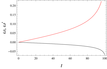
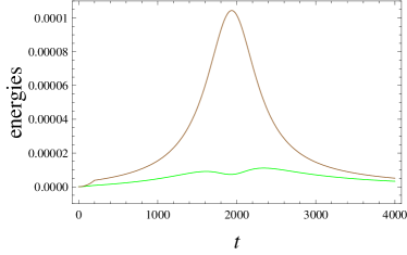
Figs. 1 refer to repelling and that start to move from a fixed distance, with zero velocities for , i.e. in (39). (Here the full 3d case reduces to the considered 1d situation.)
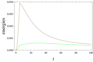
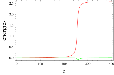
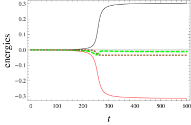
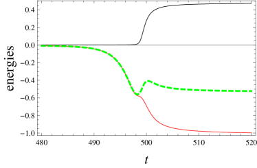
Figs. 2 describe a classical analogue of the annihilation process: two attractive particles and fall into each in a finite time; their evolution again starts from a fixed distance and with zero velocities.
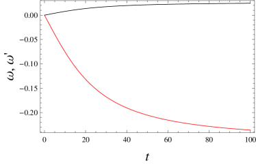
Figs. 3 show a scattering process of repelling particles: runs on which is at rest initially. For scattering processes—where particles are free both initially and finally—(35–38) predict elastic collision, if conditions discussed around (31) hold, i.e. the radiation reaction can be neglected.
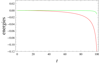
Figs. 4 show a specific elastic collision, where no energy transfers takes place between initial and final (asymptotically-free) states, but there is a non-trivial work-exchange at intermediate times.
Figs. 1, 1, 2, 3, 4 and 4 show that (47) holds with a good precision provided that is sufficienly large. Everywhere we assume (41): Figs. 1, 2 and 3 demonstrate that even for modestly large values of the motion of is weakly perturbed by .
The definition of work is clarified via Figs. 1 and 4: they show that is a better conserved quantity than ; cf. (43, 44). Hence the definition (46, 47) is selected by the approximate conservation law argument.
Figs. 1, 1 and 2 show that for a range of initial times is strictly conserved. Hence (47) does not hold and no work can be defined via (46). This relates to the fact that for parameters of Figs. 1 and 2 the particles and have zero velocities for ; cf. (39). Due to retardation each particle sees a fixed neighbor for some initial time. This leads to conservation of for those times. Thus, this example illustrates the causal behavior of work, a desirable feature ensured by the Lorenz gauge. It is absent for the Coulomb gauge (9), where propagates instantaneously. This example also shows that the work cannot be defined only via (46).
Another scenario for violating (47) is seen for attracting particles that approach each other closely; see Fig. 2. Now the inter-particle distance becomes comparable with (31). Hence the self-force cannot be neglected, and the considered dynamics is not applicable.
For the elastic collision displayed in Figs. 4 the initial overall kinetic momentum is zero . Hence it is zero also finally and there is no overall energy transfer. But Fig. 4 shows that the work is non-trivial at intermediate times: first the work flows from to , and then goes back by the same amount.
V Work in the presence of the self-force
So far we neglected the self-force (that includes the radiation reaction force) assuming that (31) holds. In particular, (31) restricts velocities of and . Now we get rid of this limitation and show that the first law (46, 47) still holds. Instead of (35, 36) we get from Appendix H in the 1d situation
| (50) | |||
| (51) |
Technically, (V, 51) can be solved only from the future conditions for coordinates, velocities and accelerations kos ; glass ; baylis_retarded . This fact has to do with the structure of the self-force. Hence we pose future conditions
| (52) | |||
| (53) |
and numerically integrate back employing a self-consistent method; see Appendix G. Similar methods were discussed in travis ; hsing . The existence and uniqueness of such (Cauchy) solutions are not generally known 888 There are simple examples of delay-differential equations for which the forward solution [defined e.g. via (39)] is unique, but the backward solution either does not exist or it is not unique driver_book ; book_numerics ; raju . . There are only certain partial results driver_back ; travis ; hsing ; zhdanov , e.g. that the solution exists and it is unique for the 1D repelling case, , if the the final separation is sufficiently large kirpich . We thus focus on this situation. Hence the final time is so large that the particles do not interact for and for .
Figs. 5 and 5 display our results for energy changes (43, 44) obtained from solving (V, 51, 37, 38, 52) numerically.
Fig. 5 shows that (47) holds, and the causality of the energy flow is well-visible: when the energy transfer starts (at ), first decreases, and then increases to a slightly smaller value: the transferred energy (work) first goes out of —hence decreases—and then it arrives at . The small mismatch between those initial and final values is due to the energy that is radiated away. This energy is determined from the overall kinetic energy difference between initial and final times, because at those times the particles are (asymptotically) free. For parameters of Fig. 5 the radiated energy is small.
Fig. 5 presents a situation, where the velocities are sufficiently large and the radiation is essential. The main message of Fig. 5 is that the processes of radiation and energy transfer are well-separated. This appears to be a general feature of 1d collisions under (41). First the radiation is emitted from : decreases, while ; see Fig. 5. No work is done at those times and (47) does not hold. At somewhat later times, and start to change so that (47) holds; see Fig. 5. The work is exchanged causally: first the energy leaves and both and decrease. Afterwards, and increase; see Fig. 5. The validity of (46, 47) is illustrated as
where and in Fig. 5. Hence most of the work is exchanged in the time-interval .
VI Summary
We started by arguing that the problem of defining and interpreting the thermodynamic work done on a charged particle by time-dependent electromagnetic field (EMF) is still open. In particular, the definition of the thermodynamic work is not automatic, since the time-dependent Hamiltonian (4) of the particle is not gauge-invariant. Hence deeper physical reasons are needed for coming up with a consistent definition of work. We stress that previous attempts landau ; kos ; kobe ; sipe ; wang_pra did not resolve this problem. In particular, it was not clear how to formulate the first law (that relates the work to the energy of the EMF-source), and how to connect with the mechanic work (force times displacement). All these issues are relevant for relativistic statistical thermodynamics thermo_rel .
The solution of the problem was sought along the following lines:
– The definition of work ought to emerge from a consistent energy-momentum tensor of the overall system (particles+EMF). In particular, this ensures that the definition is relativistically covariant. The standard energy-momentum tensor of EMF does not apply to this problem, since it implies that the particle does not have a potential energy and hence indirectly supports the choice of the temporal gauge that leads to unacceptable conclusions for the definition of the thermodynamic work; see section I.
– The definition should hold the first law (work-energy theorem) that relates the energy of the work-recipient with the energy of the work-source.
We carried out this program—within lacunae listed below—and showed that the physically meaningful definition emerges from the Lorenz gauge of EMF. It comes from the energy-momentum tensor (for matter+EMF) that is proposed in section II. This tensor is gauge-invariant and holds several necessary features. Its differences and similarities with the standard energy-momentum tensor are discussed in section II and Appendix B. The thermodynamic work can be defined via the particle’s Hamiltonian in the Lorenz gauge. To an extent we were able to check, it is only in this gauge that the thermodynamic work is relativistically consistent and relates to the gauge-invariant kinetic energy of the source of EMF. The latter can also be recovered as the mechanic work done by Lorentz force acting on the source, thereby establishing a relation between the thermodynamic and mechanic work.
Our motivation was and is to understand how to define work for particles interacting with/via a non-stationary EMF. Besides its obvious importance in non-equilibrium statistical mechanics,
Several questions remain open.
First, whether the first law (47) can be verified analytically. The issue here is that delay-differential equations that govern relativistic dynamics are notoriously difficult to study analytically driver_book ; book_numerics . The existing perturbative methods, which can employ (41) as a starting point, focus either on the weakly-coupled situation synge or on the long-time limit bel . Both these limits are not especially interesting for verifying (47). An analytical derivation can also clarify whether there are other gauges that hold the conservation law (47) with at least the same precision as the Lorenz gauge does.
Second, we verified the first law (47) for retarded dynamics of two coupled charges either in the limit where the radiation reaction is negligible (but the dynamics is still relativistic), or when the processes of work exchange and radiation are separated in time. (The latter is typical for 1d collisions). The proper generalization of (47) for a situation when the work exchange and radiation take place simultaneously is not clear yet.
Third, while the notion of work relates to the energy transfer, it should be interesting to study the momentum transfer along the above lines.
Fourth, our consideration is classical. We expect it to apply to the semiclassical situation, where a non-relativistic quantum system interacts with a classical EMF. But the quantum relativistic situation is not clear; in this context see Ref. silenko for a recent discussion of energy changes described by the Dirac’s equation.
Acknowledgements
We thank K.V. Hovhannisyan and A. Melkikh for suggestions. R. Kosloff, R. Uzdin and A. Levy are thanked for a seminar, where the subject of this paper was discussed. A.E.A. was supported by COST Action MP1209. Both authors were partially supported by the ICTP through the OEA-AC-100.
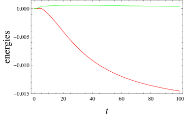
(a) The energy difference of the light particle (red) and the sum of this energy and the kinetic energy of the heavy particle (green); cf. (46, 47).
(b) (green) and (brown). The former quantity is conserved better.
(c) The velocity () of the light (heavy) particle is shown by red (black) curve.
(a) (red) and (green).
(b) (red) and (black); cf. Figs. 1–1.
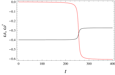
(a) (red) and (green).
(b) (red) and (black).
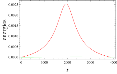
(a) Red (upper) curve . Green (lower) curve: ; cf. Fig. 1.
(b) Green (lower) curve: . Brown (upper) curve: .
(a) Final conditions are given by (52, 53): , , , . Equations of motion (V, 51) predict initial conditions: , .
Red (lower) line: . Black (upper) line: . Green dashed line: . Brown dotted line: the sum of the Larmor’s rates ; see Appendix H.
(b) , , , ; , . Red (lower) line: . Black (upper) line: . Green dashed line: . Note that the energy radiation and energy transfer are separated from each other.
References
- (1) R. Balian, From Microphysics to Macrophysics, I (Springer, Berlin, 1992).
- (2) G. Lindblad, Non-Equilibrium Entropy and Irreversibility (D. Reidel, Dordrecht, 1983).
- (3) G. Mahler, Quantum Thermodynamic Processes (Pan Stanford, Singapore, 2015).
- (4) R.L. Lehrman, Phys. Teach. 11, 15 (1973).
- (5) H.S. Leff and A.J. Mallinckrodt, Am. J. Phys. 61, 121 (1993).
- (6) M. Esposito, U. Harbola, and S. Mukamel, Rev. Mod. Phys. 81, 1665 (2009).
- (7) C. Jarzynski, Eur. Phys. J. B 64, 331 (2008).
- (8) M. Campisi, P. Hanggi, and P. Talkner, Rev. Mod. Phys. 83, 771 (2011).
- (9) P. Skrzypczyk, A. J. Short, S. Popescu, Nat. Commun. 5, 4185 (2014).
- (10) A.E. Allahverdyan, Phys. Rev. E 90, 032137 (2014).
- (11) R. Gallego, J. Eisert, and H. Wilming, Defining work from operational principles, arXiv:1504.05056.
- (12) P. Talkner and P. Hanggi, Aspects of Work, arXiv:1512.02516.
- (13) F. Plastina et al., Phys. Rev. Lett. 113, 260601 (2014).
- (14) A. E. Allahverdyan, K. V. Hovhannisyan, D. Janzing, and G. Mahler Phys. Rev. E 84, 041109 (2011).
- (15) J.M.G. Vilar, and J.M. Rubi, Phys. Rev. Lett. 100, 020601 (2008); ibid. 101, 098902 (2008); ibid. 101, 098904 (2008).
- (16) L. Peliti, Phys. Rev. Lett. 101, 098903 (2008). J. Stat. Mech.: Theory. Exp. P05002 (2008).
- (17) E.N. Zimanyi and R. J. Silbey, J. Chem. Phys. 130, 171102 (2009).
- (18) J.M.G. Vilar, and J.M. Rubi, J. Non-Equilib. Thermodyn. 36, 123 (2011).
- (19) J. Horowitz and C. Jarzynski, Phys. Rev. Lett. 101, 098901 (2008).
- (20) L.D. Landau and E.M. Lifshitz, The Classical Theory of Fields, 4th ed. (Pergamon Press, Oxford, 1975).
- (21) B. Kosyakov, Introduction to the Classical Theory of Particles and Fields (Springer, Berlin, 2007).
- (22) K.-H. Yang, Annals of Physics, 101, 62 (1976).
- (23) D.H. Kobe, E.C.T. Wen and K.H. Yang, Phys. Rev. D 26, 1927 (1982). D.H. Kobe and K.-H. Yang, J. Phys. A: Math. Gen. 13, 3171 (1980).
- (24) J. A. Sanchez-Monroy, J. Morales, and E. Zambrano, Energy operator for non-relativistic and relativistic quantum mechanics revisited, arxiv.org/1208.1425.
- (25) D. J. Griffiths, Am. J. Phys. 80, 7 (2012).
- (26) E. Leader and C. Lorcé, Phys. Rep. 541, 163 (2014).
- (27) H. R. Reiss, Limitations of gauge invariance, arXiv:1302.1212v1.
- (28) H. R. Reiss, J. Mod. Optics 59, 1371 (2012).
- (29) J. E. Sipe, Phys. Rev. A, 27, 615 (1983)
- (30) W.-M. Sun, X.-S. Chen, X.-F. Lü, and F. Wang, Phys. Rev. A, 82, 012107 (2010).
- (31) R.P. Feynman, R.B. Leighton and M. Sands, The Feynman Lectures on Physics (Addison-Wesley, Reading, MA, 1964); chapter 27.
- (32) J. Slepian, J. Appl. Phys. 13, 512 (1942). C.S. Lai, Am. J. Phys. 49, 841 (1981). P. C. Peters, Am. J. Phys. 50, 1165 (1982). R. H. Romer, Am. J. Phys. 50, 1166 (1982). D. H. Kobe, Am. J. Phys. 50, 1162 (1982). U. Backhaus and K. Schafer, Am. J. Phys. 54, 279 (1986) C.J. Carpenter, IEE Proc. 136, 55 (1989).
- (33) C. Jeffries, SIAM Rev. 34, 386 (1992).
- (34) A. M. Stewart, Eur. J. Phys. 24, 519 (2003).
- (35) B.J. Wundt and U. D. Jentschura, Annals of Physics, 327 1217 (2012).
- (36) J.A. Heras, Eur. J. Phys. 32, 213 (2011). J.A. Heras, Am. J. Phys. 75, 176 (2007).
- (37) J. A Heras and G. Fernandez-Anaya, Can the Lorenz-gauge potentials be considered physical quantities?, arXiv:1012.1063v1.
- (38) V. P. Dmitriyev, Eur. J. Phys. 25, L23 (2004).
- (39) H.E. Puthoff, Electromagnetic Potentials Basis for Energy Density and Power Flux, arxiv.org/pdf/0904.1617.
- (40) N.N. Bogoliubov and D.V. Shirkov, Introduction to theory of Quantized Fields (J. Wiley, NY, 1980).
- (41) E. Fermi, Rend. Lincei 9, 881 (1929).
- (42) A.B. van Oost, Eur. Phys. J. D, 8, 9 (2000).
- (43) G. Rousseaux, Europhys. Lett. 71 15 (2005).
- (44) J. Larsson, Am. J. Phys. 75, 230 (2007).
- (45) L-C. Tu, J. Luo and G.T. Gillies, Rep. Prog. Phys. 68, 77 (2005).
- (46) S. Deffner and A. Saxena, Phys. Rev. E 92, 032137 (2015).
- (47) J.I. Jimenez-Aquino, F.J. Uribe and R.M. Velasco, J. Phys. A 43, 255001 (2010).
- (48) A. Saha and A. M. Jayannavar, Phys. Rev. E 77, 022105 (2008).
- (49) P. Pradhan, Phys. Rev. E 81, 021122 (2010).
- (50) A. Saha, S. Lahiri, and A.M. Jayannavar Modern Physics Letters B 24, 2899 (2010)
- (51) A. Chubykalo, A. Espinoza, R. Tzonchev, Eur. Phys. J. D 31, 113 (2004).
- (52) J.L. Synge, Proc. Roy. Soc. London A 177, 118 (1940).
- (53) R.C. Stabler, Phys. Lett. 8, 185 (1964).
- (54) F.H.J. Cornish, Proc. Phys. Soc. 86, 427 (1965).
- (55) D. Leiter, J. Phys. A, 3, 89 (1970).
- (56) R.G. Beil, Phys. Rev. D, 12, 2266 (1975)
- (57) J. Franklin and C. LaMont, Brazilian Journal of Physics 44, 119 (2014).
- (58) S.B. Kirpichev and P. A. Polyakov. Journal of Mathematical Sciences, 141, 1051 (2007).
- (59) R.D. Driver, Ann. Phys. 21, 122 (1963).
- (60) R.D. Driver and M.J. Norris, Ann. Phys. 42, 347 (1967).
- (61) R. D. Driver, Ordinary and Delay Differential Equations (Springer-Verlag, New York, 1977).
- (62) A. Bellen and M. Zennaro, Numerical methods for delay differential equations (Oxford University Press, Oxford, 2003).
- (63) C.K. Raju, Time: Towards a Consistent Theory (Kluwer Academic, Dordrecht, 1994).
- (64) J. Huschilt, W. E. Baylis, D. Leiter, and G. Szamosi, Phys. Rev. D 7, 2844 (1973).
- (65) J. C. Kasher, Phys. Rev. D 12, 1729 (1975).
- (66) R.D. Driver, Phys. Rev. 178, 2051 (1969).
- (67) S.P. Travis, Phys. Rev. D 11, 292 (1975).
- (68) D.-P. Hsing, Phys. Rev. D 16, 974 (1977).
- (69) V.I. Zhdanov, J. Phys. A: Math. Gen. 24, 5011 (1991).
- (70) P.C. Aichelburg and H. Grosse, Phys. Rev. D 16, 1900 (1977).
- (71) L. Bel and J. Martin, Phys. Rev. D 8, 4347 (1973).
- (72) E. M. Pugh and G. E. Pugh, Am. J. Phys. 35, 153 (1967).
- (73) V. Fock and B. Podolsky. Sov. Phys 1, 801 (1932).
- (74) A.V. Gritsunov, Radioelectronics and Communications Systems, 52, 649 (2009).
- (75) L. Allen, M.J. Padgett, and M. Babiker, Progress In Optics, XXXIX, 39, 291 (1999).
- (76) A. Gamba, Am. J. of Phys. 35, 83 (1967).
- (77) V.N. Strel’tsov, Foundations of Physics, 6, 293 (1976).
- (78) A. Trautman, Nature, 242, 7 (1973).
- (79) D.W. Sciama, Mathematical Proceedings of the Cambridge Philosophical Society, 54, No. 01 (Cambridge University Press, 1958).
- (80) K. Hayashi and A. Bregman, Annals of Physics, 75, 562 (1973).
- (81) Relativistic statistical thermodynamics is a vast and controversial subject with many contributions over the last 110 years. We cite only three recent reviews: M. Requardt, Thermodynamics meets Special Relativity - or what is real in Physics? arXiv preprint arXiv:0801.2639. J. Dunkel and P. Hanggi, Phys. Rep. 471, 1 (2009). M. Przanowski and J. Tosiek, Physica Scripta, 84, 055008 (2011).
- (82) A.M. Gabovich and N. A. Gabovich, Eur. J. Phys. 28, 649 (2007).
- (83) E. N. Glass, J. Huschilt, and G. Szamosi, Am. J. Phys. 52, 445 (1984).
- (84) J. Huschilt, W. E. Baylis, Physical Review D 13, 3256 (1976).
- (85) A. J. Silenko, Physical Review A 91, 012111 (2015).
- (86) G. Rousseaux, Ann. Fond. Louis de Broglie 28, 261 (2005).
- (87) G. Giuliani, Eur. J. Phys. 31, 871 (2010).
- (88) V.B. Bobrov, S.A. Trigger, G.J.F. van Heijst, P.P.J.M. Schram, Aharonov-Bohm effect, electrodynamics postulates, and Lorentz condition, arXiv:1306.6736.
Appendix A Gauge-freedom of non-relativistic time-dependent Hamiltonian
The Hamiltonian (1) can be deduced from a Lagrangian via landau ; kos
| (54) |
The Lagrange equations stay intact if instead of one uses another Lagrangian :
| (55) |
The corresponding Hamiltonian
| (56) |
differs from (54) by a factor that is formally similar to the scalar potential in (4). Hence formally the time-dependent Hamiltonian is not defined uniquely.
For the considered non-relativistic situation this non-uniqueness is straightforward to resolve: one finds the time-independent (non-relativistic!) Hamiltonian for the particle and the work-source together, e.g.
| (57) |
where and are the canonical momentum and coordinate of the work-source. No issue similar to (56) arises in (57), because (57) is time-independent (one can still add to (57) a constant). Then the physical time-dependent Hamiltonian for the particle is found by neglecting its backreaction onto the source: .
Appendix B Standard forms of the energy-momentum tensor
Two versions of the energy-momentum tensor of electromagnetic field (EMF) are known in literature landau ; kos
| (58) | |||
| (59) | |||
| (60) |
is deduced from the standard Lagrangian of EMF landau ; see (71, 74) in Appendix C. is obtained from via the so called Belinfante method that renders a symmetric and explicitly gauge-invariant expression landau .
1. First we focus on comparing (58) with (18, 19), because (58) is widely accepted as the correct energy-momentum tensor. Then we turn to discussing (59).
1.1 Eq. (58) does not allow to introduce potential energy for particles [cf. (22, 24)], because the full conserved energy-momentum tensor of the EMF+matter is defined as [cf. (16)] landau
| (61) |
Hence according to (58, 61) the matter has only kinetic energy, as can be verified in detail by working out (58) analogously to (21–24). This is why (58) indirectly supports the choice of the temporal gauge .
1.2 Recall that according to (58), is energy density, and
| (62) | |||||
is the energy current (Poynting vector), and is the momentum density.
The Poynting vector is non-zero also for time-independent fields. This is a known controversy in the standard definition of the EMF energy current: stationary fields—e.g. created by a constant change and permanent magnet, which do not require any energy cost for their maintenance—would lead to permanent flow of energy and constant field momentum feynman ; jeffries ; pugh . In contrast, (23) is zero for time-independent fields puthoff . This is an advantage.
We are not aware of direct experimental results which would single out a unique expression for EMF energy current feynman ; jeffries ; slepian . Some experiments point against the universal applicability of the Poynting vector for the EMF energy flow chub .
1.3 Eq. (58) does not allow a clear-cut separation between the orbital momentum and spin of EMF. Indeed, due to , we get for a free EMF landau
| (63) |
Now is conserved, but it has the form of orbital momentum; sometimes it is also interpreted as the full angular momentum leaving unspecified the separate contributions of orbital momentum and spin landau 999Such quantities can be introduced at the level of ; see e.g. lorce_review . But this introduction is ad hoc; cf. (96, 95, 78, 80).. In contrast, (18, 19) lead to well-defined expressions for the angular momentum and spin that are conserved separately for a free EMF; see Appendix E. This Appendix also explains that when EMF couples to matter only the sum of the full orbital momentum (including that of matter) and the EMF spin is conserved.
1.4 Eq. (58) and (18, 19) lead to the same predictions for the (space-integrated) conserved quantities. Indeed, using the Lorenz gauge (10) and the equation of motion (14) for we get from (58, 18):
| (64) | |||
| (65) |
Note that (64) is not the usual freedom associated with the choice of the energy-momentum tensor landau . That freedom amounts to , which clearly does not hold with (65).
Relations amount to conservation of and in time. More generally, such a conservation law may be absent, e.g. when some non-electromagnetic forces act on the matter.
At any rate, we want to show that and do predict the same values for the full (space-integrated) energy-momentum of the matter+EMF. To this end, consider from (64, 65) the difference of the two predictions:
| (66) |
The second term in (66) contains full space-derivatives and amounts to zero under standard boundary conditions. Also, amounts to full space-derivatives,
| (67) |
where we used the Lorenz gauge condition (10). Hence (67) implies that . Thus, we get from (66)
| (68) |
1.5 Eq. (58) predicts a non-negative expression
| (69) |
for the energy density of EMF landau . In contrast, according to (18) the energy density of EMF is generally not positive. It is positive for stationary fields, and it is positive for a radiation emitted by a point particle, where (18) and (58) agree with each other; see Appendix D. The non-positivity should not be regarded as a drawback, e.g. because once for point particles the diverging terms for (58) are renormalized away, the energy density of EMF is not anymore strictly positive.
1.6 Another difference between (58) and (18) for a free EMF is that the zero-trace relation is always true, while is generally not zero; cf. (19)]. Now is generally related to the zero mass of photon. For photons we also get that ; see Appendix D. However, it is not generally true that a superposition of two or more photons (e.g. bi-photon) has a zero-mass; see e.g. gabovich . Physically, this means that we should not expect the zero-trace relation for an arbitrary EMF.
2. We now turn to discussing the features of (59).
2.1 Eq. (59) is non-symmetric even for the free EMF. Hence the desired relation between the energy current and momentum density is generally violated: . This is not physical.
2.2 The symmetry of (59) for a free EMF also means that if one introduces the orbital momentum as , it is generally not conserved: . This is not physical.
2.3 Eq. (59) is neither explicitly gauge-invariant, nor it allows to single out any specific gauge 101010This point can be reformulated as follows lorce_review . It is based on separating the full potential into a physical (i.e. gauge-invariant) part and the pure gauge: , where lorce_review . Expectedly, the modified (i.e. gauge-invariant) analogue of (59) is given by the same expression, where . The modified expression is now gauge-invariant, but is still not unique, because now there is a freedom in choosing . .
Appendix C Fermi’s Lagrangian for free EMF
The purpose of this Appendix is to derive (19) from the Fermi’s Lagrangian for a free classical electro-magnetic field (EMF) bogo ; fermi ; oost . The standard Lagrangian reads
| (71) |
where is the 4-potential.
For the Lorenz gauge (10), an alternative Lagrangian was proposed by Fermi fermi ; bogo ; oost . It is obtained from (71) upon using (10) and neglecting full derivatives
| (72) |
The equations of motion are
| (73) |
which are consistent with the Lorenz gauge (10). The latter is to be considered as a condition imposed on (72).
Given (72) and recalling the standard expression for the the energy-momentum tensor landau ; bogo
| (74) |
we obtain from (72):
| (75) |
where is the Kroenecker delta. Eqs. (75, 73) show that the tensor is symmetric and holds energy-momentum conservation
| (76) | |||
| (77) |
The invariance of a Lagrangian under rotations implies the following general relation between the energy-momentum tensor and angular momentum tensor bogo :
| (78) | |||||
| (79) |
where is given by (74), is the internal angular momentum (spin), while is the orbital momentum. Using (72) we obtain for the spin tensor bogo ; oost
| (80) |
Employing (73, 76, 77) we get that the angular momentum and spin tensor are conserved separately bogo ; oost :
| (81) |
as should be for a free field. The symmetry (76) is crucial for the existence of two separate conservation laws (81).
The standard approaches to the energy-momentum tensor of EMF are recalled in Appendix B. The spin and orbital momentum of EMF is reviewed in lorce_review ; babi .
Appendix D Energy momentum-tensor for free radiation
Here we discuss the energy-momentum tensor (19) for free radiation. Within this appendix we put .
Consider a charge moving on a world-line . Define for the 4-velocity. Recall that . Let and be defined as follows
| (82) | |||
| (83) |
Given an observation event with 4-coordinates , there is a unique point , so that the light signal emitted from a reached . Define using (82, 83) kos :
| (84) | |||
| (85) |
When changes, changes as well. Hence there is a problem of calculating derivatives kos . There are 3 main formulas here (recall that ):
| (86) | |||
| (87) | |||
| (88) |
To derive (86, 87), note from (84): . This relation together with implies: . Together with (85) this leads to (86) and then to (87). Eq. (88) is deduced from using .
The Lienard-Wichert potential of a charge reads
| (89) |
| (90) | |||||
| (91) | |||||
| (92) | |||||
| (93) | |||||
| (94) |
These expressions determine from (19) the energy-momentum tensor of EMF.
Note that the right-hand-side of (92) is the only term that scales as . This is the term responsible for the energy-momentum of the emitted radiation. It coincides with the radiation energy-momentum tensor obtained from the standard expression (58) kos . In particular, it is symmetric and has zero trace due to (83).
Appendix E Angular momentum
Here we shall connect the energy-momentum tensor to the angular momentum tensor.
It is seen from (18) that is not symmetric: . This asymmetry has a physical meaning and it relates to the spin of EMF 111111A non-symmetric energy-momentum tensor implies a generalized gravity; see, e.g. trautman ; sciama ; bregman for examples of such theories. . Recall the following general relation between the orbital momentum tensor and energy-momentum tensor landau ; bogo
| (95) |
The orbital momentum of matter is already included into . Due to , the orbital momentum is not conserved: . This is natural, since it is the full angular momentum (orbital+spin of EMF) that should be conserved. We can thus deduce the spin tensor from the conservation law
| (96) |
Eqs. (13–96) and the fact that should be a quadratic function of imply
| (97) |
This expression has formally the same shape as the spin tensor derived in bogo ; oost for a free EMF via the Fermi’s Lagrangian; see Appendix C.
Hence the matter-field coupling leads (as expected) to exchange (96) between the orbital momentum and the spin. If this coupling is absent, then is symmetric; hence and are conserved separately. These two points—conservation of under matter-EMF coupling and separate conservation of and for free EMF—are specific features of (96–97) that distinguish it from other proposals for angular momentum of EMF; see lorce_review ; babi for a review of those proposals.
Appendix F Derivation of (35–38)
Consider two interacting point particles and ; we denote their parameters by primed and unprimed letters. In (13, 15), the current divides into two contributions, each of them is conserved separately
| (98) |
The EMF field in (14, 15) also divides into two parts:
| (99) | |||
| (100) |
Hence () is created by ().
Equations of motion for and are deduced from (15) noting that the self-interaction is neglected and the point-particle limit is taken; cf. (29, 30). These equations read synge ; driver ; driver_existence ; stabler ; cornish ; leiter ; beil ; franklin ; kirpich :
| (101) |
where
| (102) | |||
| (103) |
Thus the following (self-interaction-excluded) energy-momentum tensor is conserved [cf. (18)]
| (104) | |||
| (105) |
where and are the energy-momentum tensors of and ; see (16).
As usual, we shall select the retarded (Liénard-Wiechert) solutions of (100); see landau ; kos and Appendix D. In contrast to that diverges in the point-particle limit, is already a convergent tensor, i.e. the energy of EMF and particles can be calculated via .
Appendix G Solving self-consistently delay-differential equations
1. Let us explain how to solve (35–39). The method described below was first suggested in synge ; see also franklin for a recent discussion.
We start with an initial function that holds ; cf. (39). Then (35, 37) become ordinary differential equations for and . They are solved for with initial conditions and from (40); cf. (39). The solution is denoted by . This function is extended to via (39): .
Next, is put into (36, 38), and these equations are solved for , and from (40). The solution is again extended to via (39): . Iterations are continued till convergence.
Now the initial function is defined for so that it holds (52, 53). For solving (V, 37) we need to know . It is found from (34), i.e. from
| (116) |
Hence this initial condition will change from iteration to another. Now (V, 37) can be solved as ordinary differential equations backward in from to some . Then the solution is continued to by assuming that for . This assumption is needed, because it is impossible to integrate numerically from till . Effectively, this means that the particles did not interact in the remote past; or (alternatively) that they interacted so strongly that for .
Overall, the solution defines with which we repeat the above step for (51, 38), e.g. is put into (51, 38), and now we have instead of (116): . The backward solution of ordinary-differential (51, 38) is continued as for . Once iterations converged, we assure by direct replacement that (V, 51, 37, 38) do hold for .
Appendix H Self-force
The electrodynamic self-force adds to (101) landau ; kos ; glass :
| (117) | |||
| (118) |
Constraints in (117, 118) are ensured due to and , ; cf. (11). Eqs. (117, 118) lead to (V, 51) via (106–111).
Note the following interpretation of (117) kos ; glass :
| (119) | |||
| (120) |
It was suggested that can be related to the emitted (radiated away) 4-momentum kos ; glass (Larmor’s rates), while is to be related with the bound 4-momentum, i.e. the momentum of an effective “cloud” around the particle kos ; glass .
We did not find a serious support for these interpretations for the two-particle dynamics; e.g. Fig. 5 shows that the radiated energy is not given by the sum of integrated Larmor’s rates. Another attempt to check these interpretations is to correct the kinetic energies in (45, 42) by the “cloud” energies
and then to see whether leads to a better conservation law. We found that the corrected kinetic energies do not generally lead to a better conservation law than (47).