The global uniqueness and $C^{1}$-regularity of geodesics in expanding impulsive gravitational waves

Abstract

We study geodesics in the complete family of expanding impulsive gravitational waves propagating in spaces of constant curvature, that is Minkowski, de Sitter and anti-de Sitter universes. Employing the continuous form of the metric we rigorously prove existence and global uniqueness of continuously differentiable geodesics (in the sense of Filippov) and study their interaction with the impulsive wave. Thereby we justify the “$C^{1}$-matching procedure” used in the literature to derive their explicit form.

1 Introduction

Impulsive gravitational waves for some time now have served as simple yet interesting models of exact radiative spacetimes in Einstein’s theory describing violent but short bursts of gravitational radiation, see e.g. [1, Ch. 20]. Also they are spacetimes of low regularity described either by a (locally Lipschitz) continuous metric or even by a distributional metric. Consequently, these geometries are also interesting from a mathematical point of view, raising questions in non-smooth Lorentzian geometry — a topic that has recently attracted some attention (e.g. [2, 3, 4, 5, 6]).

Indeed, in the case of impulsive pp-waves [1, Sec. 20.2], i.e., nonexpanding impulsive waves in Minkowski space, the discontinuous transformation between the distributional Brinkman form of the metric and the Lipschitz continuous Rosen form has been put into the mathematically rigorous framework of nonlinear distributional geometry in [7]. At the heart of this result lies a good mathematical understanding of the geodesics in both forms of the metric. With the long-term objective in mind to generalise this result to nonexpanding impulsive waves propagating on all backgrounds of constant curvature with any cosmological constant $\Lambda$, recently their geodesics have been studied in the continuous form [8] as well as in the distributional form [9] (using a 5D-formalism). In particular, in the continuous form it was essential to use a general solution concept due to Filippov [10] — well known in ODE-theory — to cope with the geodesic equation which has a discontinuous but bounded right hand side.

In this work we transfer this approach to expanding impulsive waves, see e.g. [1, Sec. 20.4–5]. More precisely, we consider the entire class of expanding impulsive waves propagating on spaces of constant curvature — Minkowski space, de Sitter and anti-de Sitter universes (with vanishing, positive and negative cosmological constant $\Lambda$, respectively). It is well known that the mathematical intricacies connected with the distributional form of the metric and its relation to the continuous form are much more severe in the expanding case. Nevertheless relevant progress has been achieved in [11, 12, 13, 14] — although partly only formal. On the other hand, using the continuous form of the metric the geodesics have been explicitly described in [15] for Minkowski background and in [16] for general $\Lambda$. Both of these works used a “$C^{1}$-matching procedure”: The geodesics of the background spacetime on both “sides” of the impulsive wave were matched on the wave surface. However, to obtain the correct number of equations to match all integration constants “before” and “behind” the wave impulse it had to be assumed — without proof — that the geodesics are continuously differentiable curves. It is the main objective of this work to supply such a proof.

We begin, however, in Section 2 with a rather detailed review of the complete class of expanding impulsive gravitational waves in spaces of constant curvature, including various methods of their construction. In particular, we collect all the main forms of the metric in a unified notation to also provide a point of reference for future work. We focus on particle motion using the continuous form of the metric in Section 3. We briefly review previous work [15, 16] and derive the equations for the real form of the metric in Section 3.1. Then, in Section 3.2 we employ the Lipschitz property of the continuous form of the metric which allows for an application of Filippov’s solution theory for ordinary differential equations with discontinuous right hand sides to solve the geodesic equations. In this way the existence and the $C^{1}$-regularity of the geodesics is obtained from a general result [17]. However, the quest for uniqueness becomes delicate since it is no longer possible to argue on general grounds (cf. [8, Sec. 3.3]) but we have to combine arguments exploiting the geometry of the spacetimes at hand with basic facts from Filippov’s theory. In particular, we provide a detailed study of the interaction of the geodesics with the wave impulse and in this way we prove in Section 3.3 that the geodesic equations possess globally unique continuously differentiable solutions. This turns the “$C^{1}$-matching procedure”​, employed in [15, 16] and reviewed in Section 4, into a mathematically valid technique to explicitly derive the geodesics that cross the impulse. Moreover, we also find (spacelike) geodesics that touch the impulse which have not been considered in the context of the matching procedure so far.

2 Exact expanding impulsive gravitational waves in spacetimes of constant curvature

Physically, impulsive gravitational waves arise most naturally as a limit of a suitable family of sandwich waves with profiles of ever “shorter duration” $\varepsilon$ which simultaneously become “stronger” as ${\varepsilon^{-1}}$. Mathematically, this amounts to a distributional limit of a sequence of sandwich profiles which converges to the profile $\delta$, the Dirac function. An impulsive gravitational wave is thus localised on a single wave-front, which is a null hypersurface.

Interestingly, there exist several alternative methods of construction of such exact expanding solutions to Einstein’s vacuum field equations. They will now be summarised and compared, together with the appropriate references to original works.

2.1 The Penrose “cut and paste” method

A fundamental geometric method for constructing impulsive (purely) gravitational spherical waves, expanding in backgrounds of constant curvature, was introduced (for flat space) by Penrose in his seminal work [18]. The general method starts with the following unified form of Minkowski (${\Lambda=0}$) or (anti-)de Sitter (${\Lambda\not=0}$) spacetime

$${\rm d}s_{0}^{2}=\frac{2\,{\rm d}\eta\,{\rm d}\bar{\eta}-2\,{\rm d}{\cal U}\,{\rm d}{\cal V}}{[\,1+\frac{1}{6}\Lambda(\eta\bar{\eta}-{\cal U}{\cal V})\,]^{2}}\,,$$ (1)

on which the transformation

$$\eta=\frac{Z}{p}\,V\,,\quad{\cal U}=\frac{Z\bar{Z}}{p}\,V-U\,,\quad{\cal V}=\frac{1}{p}\,V-\epsilon U\quad\text{with}\quad p=1+\epsilon Z\bar{Z}\,,\quad\epsilon=-1,0,+1$$ (2)

is applied. The background spacetimes of constant curvature thus take the form

$${\rm d}s_{0}^{2}=\frac{2\,(V/p)^{2}\,{\rm d}Z\,{\rm d}\bar{Z}+2\,{\rm d}U\,{\rm d}V-2\epsilon\,{\rm d}U^{2}}{\big{[}\,1+\frac{1}{6}\Lambda U(V-\epsilon U)\,\big{]}^{2}}\,.$$ (3)

In these coordinates, the hypersurface ${U=0}$ is a future null cone $\cal N$ (a sphere expanding with the speed of light) since ${U(V-\epsilon U)=\eta\bar{\eta}-{\cal U}{\cal V}=0}$. The Minkowski or (anti-)de Sitter manifold ${\cal M}$ can thus be divided into two parts, namely ${{\cal M}^{-}(U<0)}$ inside the null cone $\cal N$, and ${{\cal M}^{+}(U>0)}$ outside of it.

The Penrose “cut and paste” construction is based on re-attaching these two parts ${{\cal M}^{-}}$ and ${{\cal M}^{+}}$ with a particular “warp” along $\cal N$, generated by an arbitrary complex valued function $h(Z)$, see Figure 1. Specifically, the Penrose junction conditions prescribe the identification

$$\Big{[}\,Z,\,\bar{Z},\,V,\,U=0_{-}\,\Big{]}_{{}_{{\cal M}^{-}}}\equiv\Big{[}\,h(Z),\,\bar{h}({\bar{Z}}),\,\frac{1+\epsilon\,h\bar{h}}{1+\epsilon Z\bar{Z}}\frac{V}{|h^{\prime}|},\,U=0_{+}\,\Big{]}_{{}_{{\cal M}^{+}}}\$$ (4)

of the corresponding points from the two re-attached parts across the expanding sphere ${U=0}$.

Figure 1: Minkowski or (anti-)de Sitter space is cut into two parts ${\cal M}^{-}$ and ${\cal M}^{+}$ along a future null cone ${\cal N}$. These parts are then re-attached with an arbitrary “warp” in which points on both sides of ${\cal N}$ are identified. Such a construction generates spherical impulsive gravitational waves expanding in these constant-curvature backgrounds.

In [18] Penrose only considered the case ${\Lambda=0}$, ${\epsilon=0}$, see also [19, 20]. The generalisation to the cases ${\Lambda\not=0}$, ${\epsilon=0}$ and ${\Lambda=0}$, ${\epsilon=+1}$ was found by Hogan in [22] and [23], respectively (see also [20] for arbitrary $\epsilon$). The completely general form (3), (4) was subsequently found by Podolský and Griffiths [11, 24, 12].

2.2 Continuous coordinates

The Penrose “cut and paste” method, although illustrative, does not provide explicit metric forms of the complete spacetimes. We now do so, following and extending Hogan [25, 23], and perform another transformation of (1), generalising (2) but still linear in $U$ and $V$, given by

$${\cal V}={\cal A}\,V-{\cal D}\,U\,,\quad{\cal U}={\cal B}\,V-\,{\cal E}\,U\,,\quad\eta\,=\,{\cal C}\,V-{\cal F}\,U\,,$$ (5)

where

$${\cal A}=\frac{1}{p|h^{\prime}|}\,,\quad{\cal B}=\frac{|h|^{2}}{p|h^{\prime}|}\,,\quad{\cal C}=\frac{h}{p|h^{\prime}|}\,,\quad{\cal D}=\frac{1}{|h^{\prime}|}\bigg{\{}\frac{p}{4}\left|\frac{h^{\prime\prime}}{h^{\prime}}\right|^{2}+\epsilon\left[1+\frac{Z}{2}\frac{h^{\prime\prime}}{h^{\prime}}+\frac{\bar{Z}}{2}\frac{\bar{h}^{\prime\prime}}{\bar{h}^{\prime}}\right]\!\bigg{\}},$$

$${\cal E}=\frac{|h|^{2}}{|h^{\prime}|}\bigg{\{}\frac{p}{4}\left|\frac{h^{\prime\prime}}{h^{\prime}}-2\frac{h^{\prime}}{h}\right|^{2}+\epsilon\left[1+\frac{Z}{2}\left(\frac{h^{\prime\prime}}{h^{\prime}}-2\frac{h^{\prime}}{h}\right)+\frac{\bar{Z}}{2}\left(\frac{\bar{h}^{\prime\prime}}{\bar{h}^{\prime}}-2\frac{\bar{h}^{\prime}}{\bar{h}}\right)\right]\!\bigg{\}}\,,$$ (6)

$${\cal F}=\frac{h}{|h^{\prime}|}\bigg{\{}\frac{p}{4}\left(\frac{h^{\prime\prime}}{h^{\prime}}-2\frac{h^{\prime}}{h}\right)\frac{\bar{h}^{\prime\prime}}{\bar{h}^{\prime}}+\epsilon\left[1+\frac{Z}{2}\left(\frac{h^{\prime\prime}}{h^{\prime}}-2\frac{h^{\prime}}{h}\right)+\frac{\bar{Z}}{2}\frac{\bar{h}^{\prime\prime}}{\bar{h}^{\prime}}\right]\!\bigg{\}}\,,$$

and ${h=h(Z)}$ is as above. Interestingly, the coefficients (6) satisfy the non-trivial identities

$${\cal C}\bar{\cal C}-{\cal A}{\cal B}=0\,,\quad{\cal F}\bar{\cal F}-{\cal D}{\cal E}=-\epsilon\,,\quad{\cal A}{\cal E}+{\cal B}{\cal D}-{\cal C}\bar{\cal F}-\bar{\cal C}{\cal F}=1\,,$$ (7)

implying ${\eta\bar{\eta}-{\cal U}{\cal V}=U(V-\epsilon U)}$. The null cone $\cal N$ is thus again located along ${U=0}$.

With the transformation (5), (6), the metric (1) of any constant curvature space becomes

$${\rm d}s_{0}^{2}=\frac{2\left|(V/p){\rm d}Z+Up\bar{H}{\rm d}\bar{Z}\right|^{2}+2{\rm d}U{\rm d}V-2\epsilon{\rm d}U^{2}}{\big{[}\,1+\frac{1}{6}\Lambda U(V-\epsilon U)\,\big{]}^{2}}\,,\ \text{with}\ H(Z)=\frac{1}{2}\!\bigg{[}\frac{h^{\prime\prime\prime}}{h^{\prime}}-\frac{3}{2}\left(\frac{h^{\prime\prime}}{h^{\prime}}\right)^{\!2}\bigg{]}.$$ (8)

Notice that (5), (6) reduce to (2) for the simplest choice ${h(Z)=Z}$ implying ${H=0}$. We now combine the line element (8) for ${U>0}$ with the metric (3) for ${U<0}$ to obtain

$${\rm d}s^{2}=\frac{2\left|(V/p)\,{\rm d}Z+U_{+}(U)\,p\,\bar{H}\,{\rm d}\bar{Z}\right|^{2}+2\,{\rm d}U\,{\rm d}V-2\epsilon\,{\rm d}U^{2}}{\big{[}\,1+\frac{1}{6}\Lambda U(V-\epsilon U)\,\big{]}^{2}}\,,$$ (9)

where ${U_{+}(U)}$ is the kink function defined as ${U_{+}(U)\equiv 0}$ for ${U\leq 0}$ and ${U_{+}(U)\equiv U}$ for ${U\geq 0}$, i.e., ${U_{+}=U\Theta(U)}$ where $\Theta$ is the Heaviside step function. This metric was presented for ${\Lambda=0}$ in [19, 26, 25, 23], for ${\Lambda\not=0}$ in [22], and in the most general form in [11, 12].

Since the kink function is Lipschitz continuous the metric (9) is locally Lipschitz in the variable $U$. Thus, apart from possible singularities of the function $H$, the spacetime is locally Lipschitz. Recall that by Rademacher’s theorem a locally Lipschitz metric $g$ (denoted by ${g\in C^{0,1}}$) possesses a locally bounded connection, and so the metric is well within the “maximal” distributional curvature framework as identified by Geroch and Traschen [28]: Indeed a metric of Sobolev regularity $H^{1}_{\mbox{\small loc}}\cap L^{\infty}_{\mbox{\small loc}}$ allows to (stably) define the curvature in distributions, see also [29, 30]. Since locally Lipschitz metrics possess no bound on the curvature (in $L^{\infty}$), the discontinuity in the derivatives of the metric introduces impulsive components in the Weyl and curvature tensors, namely ${\Psi_{4}=(p^{2}H/V)\,\delta(U)}$ and ${\Phi_{22}=(p^{4}H\bar{H}/V^{2})\,U\,\delta(U)}$. Clearly, the spacetime is thus conformally flat everywhere except on the impulsive wave surface ${U=0}$. It is a vacuum solution everywhere except at ${V=0}$ on the wave surface ${U=0}$ where a curvature singularity (“origin of the impulse”) is located, and at possible poles of the function $p^{2}H$. Hence it is most natural to only consider the region ${V>0}$ of the spacetime.

The above procedure is an explicit version of the “cut and paste” construction since by comparing the transformations (2) at ${U=0_{-}}$ with (5), (6) at ${U=0_{+}}$, we obtain exactly (4).

The geometrical meaning of the function $h(Z)$. The generating complex function ${h(Z)}$ provides a geometric interpretation of the junction conditions (4), see [19, 12]: Evaluating the ratio ${\eta/{\cal V}}$ using (2) and (5) for ${U<0}$ and ${U>0}$, respectively, we find that on the impulse

$$\frac{\eta}{{\cal V}}=Z\quad\mbox{for}\quad U=0_{-}\,,\qquad\hbox{and}\qquad\frac{\eta}{{\cal V}}=h(Z)\quad\mbox{for}\quad U=0_{+}\,.$$ (10)

By (1) we have ${\eta/{\cal V}=(x+{\hbox{i}}\,y)/(t-z)}$ in Minkowski and also (anti-)de Sitter space, see [1, Ch. 4–5] or [16]. This is the relation for a stereographic projection from the North pole of the sphere onto its equatorial plane. This permits us to represent the wave surface ${U=0}$ either as a Riemann sphere or as its associated complex plane parametrized by the coordinate $Z$. Accordingly, the Penrose junction condition (4) can equivalently be understood as a mapping on the complex plane ${Z\to h(Z)}$.

This insight can be used to construct explicit solutions: For example, we may assume that the region ${U<0}$ inside the impulse represented by ${Z=|Z|e^{i\phi}}$ covers the complete sphere, ${\phi\in[-\pi,\pi)}$. However, the range of the function $h(Z)$ in general will not cover the entire sphere outside the spherical impulse for $U>0$. In particular, the complex mapping

$$h(Z)=Z^{1-\delta}\,,$$ (11)

where ${\delta>0}$, covers the plane minus a wedge as ${\,\arg h(Z)\in[-(1-\delta)\pi,(1-\delta)\pi)}$. This represents Minkowski, de Sitter, or anti-de Sitter space with a deficit angle $2\pi\delta$, which may be considered to describe a snapped cosmic string in the region outside the spherical impulsive wave. The string has a constant tension and is located along the axis ${\eta=0}$. The corresponding metric takes the form (9) with $H$ generated from (11), i.e. $H={\textstyle\frac{1}{2}\delta(1-\frac{1}{2}\delta)}\,Z^{-2}\,,$ see [12] for more details. Also quantum fluctuations and aspects of particle creation on such expanding spherical impulsive and shock waves were analysed (in different coordinates) by Hortaçsu [26, 31] and his collaborators [32, 33, 34]. More generally one may, e.g., construct impulsive waves generated by two colliding and snapping cosmic strings [19], see also [12, 35].

Contracting and expanding impulses. Hogan in [36] has considered a natural extension in which the impulse in addition to the future null cone ${\cal N}$ is also located along the past null cone. Such a spacetime contains both imploding and exploding impulses, with a curvature singularity at the common vertex. We now extend Hogan’s construction [36] to arbitrary $\Lambda$ and ${\epsilon}$ by introducing ${V^{\prime}=V-\epsilon U}$ and modifying (9) to

$${\rm d}s^{2}=\frac{2\left|(V^{\prime}+\epsilon U)/p\,{\rm d}Z+\Big{(}U_{+}(U)\,\bar{H}+[V^{\prime}-V_{+}(V^{\prime})]\,\bar{G}\Big{)}\,p\,{\rm d}\bar{Z}\right|^{2}+2\,{\rm d}U\,{\rm d}V^{\prime}}{\big{(}\,1+\frac{1}{6}\Lambda UV^{\prime}\,\big{)}^{2}}\,.$$ (12)

Here the two complex functions $H(Z)$ and $G(Z)$ characterise the expanding and the contracting impulse, respectively. The complete null cone is now given by ${\eta\bar{\eta}-{\cal U}{\cal V}=UV^{\prime}=0}$, and the Weyl tensor components are ${\Psi_{4}=(p^{2}H/V^{\prime})\,\delta(U)}$ and ${\Psi_{0}=-\epsilon(p^{2}\bar{G}/U)\,\delta(V^{\prime})}$, with $\Psi_{4}$ and $\Psi_{0}$ representing the exploding and the imploding impulse, respectively. Such a spacetime is algebraically general. At ${U=0=V^{\prime}}$ there is a highly complicated physical singularity.

2.3 Limits of sandwich waves

We now turn to the construction of expanding impulsive waves as distributional limits of sandwich waves in a suitable family of exact radiative spacetimes — as mentioned at the beginning of this section. It was explicitly argued in [11] that the full family of solutions for expanding spherical gravitational waves can be considered to be an impulsive limit of the class of vacuum Robinson–Trautman type N solutions with a cosmological constant.

Robinson–Trautman sandwich waves. The standard metric [37, 38] of Robinson and Trautman (see also [39] and [40, 1]) reads

$${\rm d}s^{2}=2\frac{r^{2}}{P^{2}}\,{\rm d}\zeta{\rm d}\bar{\zeta}+\,2\,{\rm d}u\,{\rm d}r-\Big{(}2\epsilon+2r(\log P)_{,u}-{\textstyle\frac{1}{3}}\Lambda r^{2}\Big{)}{\rm d}u^{2}\,,$$ (13)

in which the function $P(\zeta,\bar{\zeta},u)$ has the general form [41]

$$P=\left(1+\epsilon F\bar{F}\right)\big{(}F_{,\zeta}\bar{F}_{,\bar{\zeta}}\big{)}^{-1/2},$$ (14)

where ${F=F(\zeta,u)}$ is an arbitrary complex valued function of $u$, holomorphic in $\zeta$, and ${\epsilon=-1,0,+1\,}$ determines the Gaussian curvature ${K=2\epsilon}$ of each wave surface ${u=\>}$const. on ${r=1}$, spanned by $\zeta$. For the simplest case ${F=\zeta}$ and ${\Lambda=0}$ we obtain the metric (3) of Minkowski space, with the identification ${u=U}$, ${r=V}$, ${\zeta=Z}$, and ${P=p}$.

As shown in [37, 38] and the work by Newman and Unti [42], recently reviewed and generalised in [43], the coordinates employed in (13) are the most natural ones for twist-free spacetimes, having a clear geometrical meaning: Consider any worldline $\gamma$ in flat space. At any event ${\cal P}$ on $\gamma$ construct the future null cone $C_{\tau}=\{u=\tau\}$, where $\tau$ is the parameter value of ${\cal P}$ along $\gamma$. The resulting family of null cones (locally) foliates the spacetime. Now, introduce the coordinate $r$ as the affine parameter along the null generators of $C_{\tau}$, normalised such that ${r=0}$ labels ${\cal P}\in\gamma$. Finally, introduce two spatial coordinates to label all points on the sections ${r=\>}$const. on $C_{\tau}$. In the case ${\epsilon=+1}$ this is a 2-sphere, most naturally parameterized by ${\theta\in[0,\pi]}$, ${\phi\in[-\pi,\pi)}$ via ${\zeta\equiv\tan(\theta/2)\exp(\hbox{i}\phi)}$.

The simplest choice is to consider special geodesic trajectories with velocity normalised to $-\epsilon$, i.e., a static timelike observer (${\epsilon=+1}$), a null geodesic (${\epsilon=0}$), or a spacelike (tachyonic with infinite speed) geodesic (${\epsilon=-1}$). For these choices the hypersurfaces $C_{\tau}$ are shown in Figure 2. It can be seen that the most natural choice is ${\epsilon=+1}$ which gives a (global) foliation of the spacetime. The cones nicely fit one into another and the wave surfaces at any time form concentric spheres. It is thus the best candidate for performing the impulsive limit of sandwich gravitational waves, resulting in the impulse located on a single wavefront ${u=0}$.

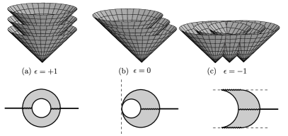
Figure 2: Upper part: The family of future null cones $C_{\tau}$ with vertices along a timelike (${\epsilon=+1}$), null (${\epsilon=0}$), or a spacelike (${\epsilon=-1}$) line foliate in three different ways Minkowski space in the Robinson–Trautman form. Analogous foliations apply to (anti-)de Sitter space, see [1]. Lower part: sandwich gravitational waves at a fixed time for different values of $\epsilon$ are indicated by the shaded regions. All wavefronts ${u=\>}$const. are spherical (hemispherical for ${\epsilon=-1}$) and expand with the speed of light. The inner region ${u<0}$ is free of topological defects, while the external region ${u>u_{1}>0}$ contains a cosmic string (thick line) which “disintegrates” within the sandwich (zigzag line), generating the wave.

The family of such sandwich waves was introduced by Griffiths and Docherty in [44] and further studied in [13] for all possible values of $\Lambda$ and signs of $\epsilon$. The metric has the Robinson–Trautman canonical form (13), (14), with the function $F(\zeta,u)$ taken to be

$$F(\zeta,u)=\zeta^{g(u)},$$ (15)

where $g(u)$ is any positive function of the retarded time $u$. Consequently,

$$P^{2}=\frac{\left[1+\epsilon(\zeta\bar{\zeta})^{g}\right]^{2}}{g^{2}(\zeta\bar{\zeta})^{g-1}}\,,\qquad(\log P)_{,u}=-\left(1+{\textstyle\frac{1}{2}}\log(\zeta\bar{\zeta})^{g}\left[\frac{1-\epsilon(\zeta\bar{\zeta})^{g}}{1+\epsilon(\zeta\bar{\zeta})^{g}}\right]\right)\frac{\>g^{\prime}}{g},$$ (16)

where ${g^{\prime}=g_{,u}}$, and ${\Psi_{4}=-\frac{1}{2}(1/r)(\zeta/\bar{\zeta})\big{(}|\zeta|^{-g}+\epsilon|\zeta|^{g}\big{)}^{2}(g^{\prime}/g)\,}$ is the only non-trivial component of the Weyl tensor. The solution is thus conformally flat (i.e., Minkowski or (anti-)de Sitter background) if and only if $g$ is a constant. In general, this is an exact Robinson–Trautman gravitational wave with an arbitrary profile determined by $g(u)$. Interestingly, the term $(\log P)_{,u}$ in (13) and also $\Psi_{4}$ are both proportional to the same wave profile, namely $g^{\prime}/g$.

The simplest sandwich-wave is obtained using the continuous function $g(u)$ given by

$$g(u)=1\hbox{\quad for\ }u<0\,,\quad g(u)=1-a\,u\hbox{\quad for\ }u\in[0,u_{1}]\,,\quad g(u)=1-a\,u_{1}\hbox{\quad for\ }u>u_{1}\,,$$ (17)

where ${a,u_{1}}$ are positive constants [44], [1, Sec. 19.2.3] so that ${g^{\prime}=-a}$ within $[0,u_{1}]$. Outside this wavezone ${g^{\prime}=0}$ so that the spacetime is (conformally) flat. However, ahead of this sandwich wave in the region ${u>u_{1}>0}$ there is a topological defect at ${\zeta=0}$ or ${\zeta=\infty}$ (since ${g<1}$) representing a cosmic string with the deficit angle ${2\pi au_{1}}$. The region ${u<0}$ behind the wave contains no such defect (because ${g=1}$). The solution (15), (17) has thus been interpreted as a breaking of a cosmic string in a conformally flat background in which the tension of the string (deficit angle) reduces uniformly to zero. Such a cosmic string decay generates a gravitational wave, see the lower part of Figure 2.

The derivative of the function $g$ given by (17) has discontinuities ${|g^{\prime}|=a}$ at ${u=0}$ and ${u=u_{1}}$, so that there are shocks on the initial and final wave surfaces of the sandwich (for discussion of spherical shocks see [20]). More general families of sandwich waves without such discontinuities in the metric and $\Psi_{4}$ can be constructed by considering smooth functions $g(u)$. Moreover, if ${g=1}$ on both sides of the sandwich, the Minkowski or (anti-)de Sitter background does not contain a cosmic string either in front of nor behind the wave.

Robinson–Trautman impulses. Using the model (17), it is easy to perform the impulsive limit of such Robinson–Trautman sandwich waves by taking the limit ${u_{1}\to 0}$, keeping ${\gamma\equiv au_{1}>0}$ fixed. This yields the function [14]

$$g(u)=1\hbox{\quad for\ }u<0\,,\qquad g(u)=1-\gamma\hbox{\quad for\ }u>0\,,$$ (18)

i.e., ${g(u)=\exp[\,c\,\Theta(u)]}$, where ${c=\ln(1-\gamma)<0}$ and $\Theta$ is the step function, in which case

$$g^{\prime}/g=c\,\delta(u)\,,$$ (19)

where $\delta(u)$ is the Dirac delta. We thus indeed obtain an impulsive gravitational wave, with the Weyl curvature tensor localised on the single wavesurface ${u=0}$. Notice that the Dirac $\delta$ also directly enters the metric via the ${(\log P)_{,u}}$ term in (16). This leads us out of the Geroch–Traschen class [28] of metrics, but due to the simple geometrical structure it is still possible to calculate the curvature as a distribution. The ansatz (15) has also been generalised to obtain sandwich and impulsive waves with a richer structure, for example two impulses or a bending string, see [13].

Alternatively, the family of Robinson–Trautman type N metrics (13) can also be expressed in terms of García–Plebański coordinates [45, 46] as

$${\rm d}s^{2}=2\,(r/\psi)^{2}\,\big{|}{\rm d}\xi-f\,{\rm d}u\big{|}^{2}+2\,{\rm d}u\,{\rm d}r-\left(2\epsilon-r\,Q-{\textstyle\frac{1}{3}}\Lambda r^{2}\right){\rm d}u^{2}\,,$$ (20)

where ${\psi=1+\epsilon\xi\bar{\xi}}$, $\,f(\xi,u)$ is an arbitrary complex valued function, holomorphic in $\xi$, and ${Q=(f_{,\xi}+\bar{f}_{,\bar{\xi}})-2\epsilon\psi^{-1}(\bar{\xi}f+\xi\bar{f})}$, see also [20, 38]. This line element is related to (13) via the transformation $\xi\equiv F(\zeta,u)$ with $F_{,u}=f(F(\zeta,u),u)$, see [47, 11]. With the specific choice (15) convenient for sandwich and impulsive waves, this corresponds to [14]

$$f(\xi,u)=(g^{\prime}/g)\,\xi\log\xi\,.$$ (21)

In particular, for (18), (19) which represents a snapping string accompanied by an impulsive spherical gravitational wave localised at ${u=0}$, the functions are

$$f=c\,\xi\log\xi\,\delta(u)\,,\qquad Q=2c\,\Big{(}1+\frac{1-\epsilon\xi\bar{\xi}}{1+\epsilon\xi\bar{\xi}}\log|\xi|\Big{)}\delta(u)\,,$$ (22)

see [14]. However, observe that the form of the metric (20) with (22) has to be considered as being only formal, since it is quadratic in $f$ and so explicitly contains a square of the Dirac $\delta$.

Finally, the Robinson–Trautman impulsive spacetimes (20) with ${f\equiv f(\xi)\,\delta(u)}$ can also be rewritten in the alternative form

$${\rm d}s^{2}=\frac{2\,(v/\psi)^{2}\,|{\rm d}\xi-f(\xi)\delta(\bar{u})\,{\rm d}\bar{u}|^{2}+2\,{\rm d}\bar{u}\,{\rm d}v-2\epsilon\,{\rm d}\bar{u}^{2}-v\,Q(\xi)\delta(\bar{u})\,{\rm d}\bar{u}^{2}}{[\,1+\frac{1}{6}\Lambda\bar{u}(v-\epsilon\bar{u})\,]^{2}}\,,$$ (23)

where the profile function ${f(\xi)}$ is any complex valued (holomorphic) function of the spatial coordinates $\xi$. This is obtained from the García–Plebański coordinates (20) by the transformation

$$r=\frac{v}{1+\frac{1}{6}\Lambda\bar{u}(v-\epsilon\bar{u})}\,,\qquad u=\int\frac{{\rm d}\bar{u}}{1-\frac{1}{6}\Lambda\epsilon\bar{u}^{2}}\quad\hbox{such that}\quad u=0\Leftrightarrow\bar{u}=0\,,$$ (24)

implying ${\delta(u){\rm d}u=\delta(\bar{u}){\rm d}\bar{u}}$, with the spherical impulse again located on the null surface ${\bar{u}=0}$. Clearly, for any ${\bar{u}\not=0}$ the metric (23) is the Minkowski or (anti-)de Sitter background in the form (3) with the identification ${\bar{u}=U}$, ${v=V}$, ${\xi=Z}$ (so that ${\psi=p}$). However, it also has to be considered as only formal since again a square of the Dirac delta enters the metric.

The relation of (23) to the continuous metric form (9) for expanding impulsive waves was found in [11]. Performing the discontinuous transformation ${x_{i}=X_{i}+\Theta(U)\,[X_{i}^{{\hbox{\tiny inv}}}(X_{j})-X_{i}\,]}$, where ${x_{i}\equiv(\bar{u},v,\xi)}$, ${X_{i}\equiv(U,V,Z)}$, and $X_{i}^{{\hbox{\tiny inv}}}(X_{j})$ are specific functions obtained by composing the inverse of (2) with (5), it is possible to put (23) formally into the continuous form (9). This relation is obvious for ${U\not=0}$ using the identity ${\bar{u}(v-\epsilon\bar{u})=U(V-\epsilon U)}$ (trivially valid for ${U<0}$ since ${x_{i}=X_{i}}$, and also for ${U>0}$ where ${x_{i}=X_{i}^{{\hbox{\tiny inv}}}(X_{j})}$ since ${\eta\bar{\eta}-{\cal U}{\cal V}=U(V-\epsilon U)}$ due to the first identity in (7)). Keeping the distributional terms arising from $\Theta$ and its derivative in the transformation, we formally obtain also the impulsive terms proportional to $\delta$ and $\delta^{2}$ in (23) with ${f(\xi)\equiv Z^{{\hbox{\tiny inv}}}(U=0)-Z}$. Of course, much technical work is still required before such a discontinuous transformation can be put into a mathematically sound context.

2.4 Impulses generated by infinitely accelerating sources

Specific expanding spherical impulses can also be obtained from exact solutions for accelerating sources in the limit of unbounded acceleration. It was realised by Bičák and Schmidt [48, 49] and corroborated by Podolský and Griffiths [50, 51] that such impulses can be obtained from the family of boost-rotation symmetric solutions [52, 53] which describe the gravitational field of uniformly accelerating objects, typically attached to conical singularities.

Limit of the Bonnor–Swaminarayan and related solutions. Of particular interest is a special case of the Bonnor–Swaminarayan solution [54, 55] described by Bičák, Hoenselaers and Schmidt in [56, 57] which represents two particles of the Curzon–Chazy type accelerating in opposite directions. In the limit of infinite acceleration such a metric can be written as

$${\rm d}s^{2}=\textstyle{\frac{1}{4}}(\tilde{v}-\tilde{u})^{2}\,e^{-\mu}\,{\rm d}\phi^{2}+\textstyle{\frac{1}{4}}(\tilde{v}+\tilde{u})^{2}\,e^{\mu}\,{\rm d}\chi^{2}-e^{\lambda}\,{\rm d}\tilde{u}\,{\rm d}\tilde{v}\,,$$ (25)

where ${\mu=-M=\>}$const., ${\lambda=\left[\,\Theta(\tilde{u}\tilde{v})-\Theta(-\tilde{u}\tilde{v})\,\right]M}$ for the two semi-infinite receding cosmic strings located along the axis ${\rho\equiv\frac{1}{2}(\tilde{u}-\tilde{v})}{=0}$. The metric is only locally bounded with $\lambda$ suffering a finite jump of $2M$ on the null cone ${\,\tilde{u}\tilde{v}=0}$ which again brings us out of the Geroch–Traschen class [28]. The resulting spacetime is locally flat except on the expanding sphere which is the impulsive gravitational wave, generated by two null particles which move apart in the flat background and are connected to infinity by two semi-infinite strings.

It is possible to perform a transformation to coordinates in which the metric is Lipschitz continuous [50]. It actually brings (25) exactly in the form of Gleiser and Pullin [21] constructed via their “cut and paste” method. Moreover, as shown in [50], this metric can be cast in the classic form (9) with a real constant function $H$, for which, however, the geometric interpretation in terms of the stereographic correspondence is more obscured.

The above construction has been extended in [50] to a much larger class of boost-rotationally symmetric spacetimes allowing to attribute an arbitrary multipole structure to the receding particles [57], which, however, vanishes in the impulsive limit.

Infinitely accelerating black holes. In the subsequent paper [51] Podolský and Griffiths also investigated null limits of another well-know class of solutions with boost-rotation symmetry, namely the C-metric. As shown in 1970 by Kinnersley and Walker [58], such a metric represents a pair of uniformly accelerating black holes, each of mass $m$. Their acceleration $A$ is caused either by a strut between the black holes or by two semi-infinite strings connecting them to infinity. In [51] the limit ${A\to\infty}$ was investigated, demonstrating that (scaling $m$ to zero such that ${mA=\>}$const.) it is again identical to the metric of a spherical impulsive gravitational wave generated either by a snapping string, or an expanding strut.

It was natural to expect that the analogous null limit of infinite acceleration ${A\to\infty}$ of a more general C-metric with a cosmological constant ${\Lambda}$ (see [59, 60, 61, 62]), would generate an expanding spherical impulsive wave (9) in the (anti-)de Sitter universe. Such limit turned out to be mathematically more involved but was finally performed in [14] using the Robinson–Trautman form extending (13) to type D spacetimes. The limit yielded exactly the impulsive metric form with ${F(\zeta,u)=\zeta^{g(u)}}$ where ${g(u)=\exp[\,c\,\Theta(u)]}$ and $c$ is determined by $mA$, that is (15), (18) and (19).

Further details on the various construction methods, related topics and references can be found in the reviews [63, 64, 1].

3 Geodesics in expanding impulsive waves

In this section we focus on geodesics in expanding spherical impulsive waves propagating in background spacetimes of constant curvature. Thereby we will exclusively use the continuous form (9) of the metric. Also previous work on geodesics in these geometries was solely concerned with this form of the metric. Note that this is in contrast to nonexpanding impulsive waves where the distributional forms of the metric have also widely been used, see [8, Sec. 3.1] for a brief overview as well as the recent work [9]. The reason is that in the expanding case the distributional forms of the metric (13), (20), and (23) are more complicated than those in the nonexpanding case and that (20) and (23), in addition, contain much wilder singularities.

Indeed, the explicit form of the geodesics in Minkowski spacetime with expanding spherical gravitational impulses were presented in [15] using the metric (9) with ${\Lambda=0}$. As indicated in the introduction the method employed was a matching procedure where the geodesics of the background on either side of the impulse were pasted together in a $C^{1}$-manner, i.e., by equating the corresponding positions and velocities at the time of interaction with the impulse at ${U=0}$. Strictly speaking, this procedure is mathematically justified only in the case of the geometrically privileged family of geodesics with ${Z=\mbox{const.}}$ while in the general case it was assumed without proof that the geodesics indeed are $C^{1}$-curves. In [16] this procedure was generalised to the ${\Lambda\not=0}$ cases. To again employ the “$C^{1}$-matching” procedure it had to be assumed that all geodesics crossing the impulsive wave actually are continuously differentiable curves. With this assumption, in all cases ${\Lambda>0}$, ${\Lambda=0}$, ${\Lambda<0}$ the general results on the explicit form of the geodesics have been obtained and employed for a physical discussion of geodesic motion in specific impulsive solutions, such as the refraction of geodesics caused by the spherical impulse generated by a snapping cosmic string, i.e., (9) with (11).

It is the main aim of this article to prove that the “$C^{1}$-matching” procedure is actually a mathematically valid technique. This, in particular, includes an argument that the geodesics are indeed curves of regularity $C^{1}$, but actually more is needed (cf. [8, Remark 4.1]). In fact, we have to prove the following facts on the geodesics in the impulsive wave spacetimes:

• the geodesics heading towards the impulse cross it,

• they are unique, and

• they are continuously differentiable, i.e., of $C^{1}$-regularity.

It is only under these circumstances that the matching of the geodesics of the background spacetimes — by equating their positions and velocities at the instant of interaction with the impulsive wave — is guaranteed to give the correct answer.

3.1 The geodesic equations

We will start out by explicitly deriving the geodesic equations in the real version of the continuous metric (9) which will also enable us to perform a detailed analysis of the form and the regularity of the resulting system of ordinary differential equations. We consider the metric in the form (9):

$${\rm d}s^{2}=\frac{2\left|(V/p)\,{\rm d}Z+U_{+}\,p\,\bar{H}\,{\rm d}\bar{Z}\right|^{2}+2\,{\rm d}U\,{\rm d}V-2\epsilon\,{\rm d}U^{2}}{\big{[}\,1+\frac{1}{6}\Lambda U(V-\epsilon U)\,\big{]}^{2}}\,,$$ (26)

where ${p=1+\epsilon Z\bar{Z}}$, ${\epsilon=-1,0,+1,}$ and again ${H(Z)=\frac{1}{2}[{h^{\prime\prime\prime}}/{h^{\prime}}-({3}/{2})({h^{\prime\prime}}/{h^{\prime}})^{2}]}$ is the Schwarzian derivative of an arbitrary complex function $h(Z)$. However, it will be more convenient to work with the real form of (26) which we obtain by setting ${Z=\frac{1}{\sqrt{2}}(X+\hbox{i}\,Y)}$, namely

$${\rm d}s^{2}\ = \frac{1}{[1+\frac{1}{6}\Lambda U(V-\epsilon U)]^{2}}\ \bigg{(}\Big{[}\frac{V^{2}}{p^{2}}+U_{+}^{2}\,p^{2}\,|H|^{2}\Big{]}({\rm d}X^{2}+{\rm d}Y^{2})$$

$$\qquad+2\,U_{+}V\Big{[}\,\Re(H)\,({\rm d}X^{2}-{\rm d}Y^{2})-2\,\Im(H)\,{\rm d}X{\rm d}Y\Big{]}+2\,{\rm d}U{\rm d}V-2\epsilon\,{\rm d}U^{2}\bigg{)}\,,$$ (27)

which we will write as

$${\rm d}s^{2}=\frac{1}{\omega^{2}(U,V)}\left(g_{ij}(U,V,X^{k})\,{\rm d}X^{i}{\rm d}X^{j}+2\,{\rm d}U{\rm d}V-2\epsilon\,{\rm d}U^{2}\right)\,,$$ (28)

where

$$\omega=1+{\textstyle\frac{1}{6}}\Lambda U(V-\epsilon U)\,.$$ (29)

Here $\Re(H)$ and $\Im(H)$ denote the real and imaginary parts of the complex valued function $H$, respectively, and $X^{i}=(X,Y)$, ${i=1,2}$. The components of $g_{ij}$ are explicitly given by

$$g_{11} =V^{2}/p^{2}+U_{+}^{2}\,p^{2}|H|^{2}+2\,U_{+}V\,\Re(H)\,,$$ (30)

$$g_{22} =V^{2}/p^{2}+U_{+}^{2}\,p^{2}|H|^{2}-2\,U_{+}V\,\Re(H)\,,$$ (31)

$$g_{12} =-2\,U_{+}V\,\Im(H)\,.$$ (32)

Observe that — apart from singularities of $pH$ — the first two components $g_{11}$, $g_{22}$ contain (in that order) a smooth term, a term which is $C^{1,1}$ (its first derivative is Lipschitz continuous), and a Lipschitz continuous term, denoted as $C^{0,1}$. The term $g_{12}$ is just Lipschitz continuous. Moreover, these three Lipschitz continuous terms in (30)–(32) are the only ingredients of critical regularity, i.e., below $C^{1,1}$. Recall that by Rademacher’s theorem, (locally) Lipschitz continuous functions are differentiable almost everywhere with derivative belonging (locally) to $L^{\infty}$. Derivatives of the metric coefficients $U_{+}$, $U_{+}^{2}$ will always be understood in this sense.

The non-trivial contravariant components corresponding to the metric (28) are

$$g^{UV}=\omega^{2}\,,\quad g^{VV}=2\epsilon\,\omega^{2}\,,\quad g^{UU}=0\,,\quad\hbox{and}\quad\omega^{2}g^{ij}\,,$$ (33)

where $g^{ij}$ is the inverse matrix to $g_{ij}$. The only non-zero Christoffel symbols of (28) are:

$$\Gamma^{U}_{\,UU}=-\frac{2}{\omega}(\omega_{,U}+\epsilon\omega_{,V})\,,\quad\Gamma^{U}_{\,ij}=\frac{\omega_{,V}}{\omega}\,g_{ij}-\frac{1}{2}g_{ij,V}\,,$$ (34)

$$\Gamma^{V}_{\,VV}=-2\frac{\omega_{,V}}{\omega}\,,\quad\Gamma^{V}_{\,VU}=2\epsilon\frac{\omega_{,V}}{\omega}\,,\quad\Gamma^{V}_{\,UU}=-\frac{2\epsilon}{\omega}(\omega_{,U}+2\epsilon\omega_{,V})\,,$$ (35)

$$\Gamma^{V}_{\,ij}=\frac{g_{ij}}{\omega}(\omega_{,U}+2\epsilon\omega_{,V})-(\epsilon g_{ij,V}+\frac{1}{2}g_{ij,U})\,,$$ (36)

$$\Gamma^{i}_{\,Vj}=-\delta^{i}_{j}\frac{\omega_{,V}}{\omega}+\frac{1}{2}g^{il}g_{jl,V}\,,\quad\Gamma^{i}_{\,Uj}=-\delta^{i}_{j}\frac{\omega_{,U}}{\omega}+\frac{1}{2}g^{il}g_{lj,U}\,,\quad\Gamma^{i}_{\,jk}=\,^{(s)}\Gamma^{i}_{\,jk}\,.$$ (37)

Here $\,{}^{(s)}\Gamma^{i}_{\,jk}$ denotes the Christoffel symbols of the “spatial metric” $g_{ij}$, and

$$\omega_{,V}={\textstyle\frac{1}{6}}\Lambda U\,,\qquad\omega_{,U}={\textstyle\frac{1}{6}}\Lambda(V-2\epsilon U)\,.$$ (38)

Observe that $\,{}^{(s)}\Gamma^{i}_{\,jk}$, $\Gamma^{U}_{\,ij}$, and $\Gamma^{i}_{\,Vj}$, are Lipschitz continuous, while the Christoffel symbols containing a $U$-derivative of $g_{ij}$, namely $\Gamma^{V}_{\,ij}$ and $\Gamma^{i}_{\,Uj}$, are merely $L^{\infty}_{\mbox{\scriptsize loc}}$. All other Christoffel symbols are at least Lipschitz continuous, hence not of critical regularity.

The geodesic equations thus take the following explicit form

$$\ddot{U} -\frac{2}{\omega}(\omega_{,U}+\epsilon\omega_{,V})\,\dot{U}^{2}+\Big{(}\frac{\omega_{,V}}{\omega}\,g_{ij}-\frac{1}{2}g_{ij,V}\Big{)}\dot{X}^{i}\dot{X}^{j}=0\,,$$ (39)

$$\ddot{V} -2\frac{\omega_{,V}}{\omega}\,\dot{V}^{2}+4\epsilon\frac{\omega_{,V}}{\omega}\,\dot{V}\dot{U}-\frac{2\epsilon}{\omega}(\omega_{,U}+2\epsilon\omega_{,V})\dot{U}^{2}$$

$$+\Big{(}\frac{g_{ij}}{\omega}(\omega_{,U}+2\epsilon\omega_{,V})-(\epsilon g_{ij,V}+\frac{1}{2}g_{ij,U})\Big{)}\dot{X}^{i}\dot{X}^{j}=0\,,$$ (40)

$$\ddot{X}^{i} -\Big{(}2\delta^{i}_{j}\frac{\omega_{,V}}{\omega}-g^{il}g_{jl,V}\Big{)}\dot{V}\dot{X}^{j}-\Big{(}2\delta^{i}_{j}\frac{\omega_{,U}}{\omega}-g^{il}g_{jl,U}\Big{)}\dot{U}\dot{X}^{j}+\,^{(s)}\Gamma^{i}_{\,jk}\dot{X}^{j}\dot{X}^{k}=0\,.$$ (41)

In terms of regularity, observe that all of the above equations contain Lipschitz continuous terms, which, from the perspective of classical ODE-theory, pose no problem at all. However, the $V$- and the $X$-equations in addition contain the $L^{\infty}_{\mbox{\scriptsize loc}}$-terms $g_{ij,U}$, which force us to go beyond classical existence theory for ODEs. Also observe that the system is “fully coupled” — in contrast to the nonexpanding case and pp -waves in particular — so that we cannot decouple either of the equations from the rest of the system.

To apply the Filippov solution theory in the following subsection, we need to rewrite the geodesic equations (39)–(41) in first order form. Thus, the resulting system is

$$\dot{U}= \ \tilde{U}\,,\qquad\dot{V}=\tilde{V}\,,\qquad\dot{X}^{i}=\tilde{X}^{i}\,,$$ (42)

$$\dot{\tilde{U}}= \ \frac{2}{\omega}(\omega_{,U}+\epsilon\omega_{,V})\,\tilde{U}^{2}-\Big{(}\frac{\omega_{,V}}{\omega}\,g_{ij}-\frac{1}{2}g_{ij,V}\Big{)}\tilde{X}^{i}\tilde{X}^{j}\,,$$ (43)

$$\dot{\tilde{V}}= \ 2\frac{\omega_{,V}}{\omega}\,\tilde{V}^{2}-4\epsilon\frac{\omega_{,V}}{\omega}\,\tilde{V}\tilde{U}+\frac{2\epsilon}{\omega}(\omega_{,U}+2\epsilon\omega_{,V})\tilde{U}^{2}$$

$$-\Big{(}\frac{g_{ij}}{\omega}(\omega_{,U}+2\epsilon\omega_{,V})-(\epsilon g_{ij,V}+\frac{1}{2}g_{ij,U})\Big{)}\tilde{X}^{i}\tilde{X}^{j}\,,$$ (44)

$$\dot{\tilde{X}}^{i}= \ \Big{(}2\delta^{i}_{j}\frac{\omega_{,V}}{\omega}-g^{il}g_{jl,V}\Big{)}\tilde{V}\tilde{X}^{j}+\Big{(}2\delta^{i}_{j}\frac{\omega_{,U}}{\omega}-g^{il}g_{jl,U}\Big{)}\tilde{U}\tilde{X}^{j}-\,^{(s)}\Gamma^{i}_{\,jk}\tilde{X}^{j}\tilde{X}^{k}\,,$$ (45)

which is now a first-order system with discontinuous right hand side.

3.2 Existence of $C^{1}$-geodesics

Geodesic equations with discontinuous right hand side have recently been solved in the class of nonexpanding impulsive gravitational waves by going beyond classical ODE-theory. More precisely, in [65] the geodesics in impulsive pp -waves have been treated using Carathéodory’s solution concept (see e.g. [10, Ch. 1]), using the fact that there the $U$-equation decouples from the rest of the system. In the case of nonexpanding impulsive waves with non-vanishing $\Lambda$, the $U$-equation is coupled to the spatial equations, which made it necessary to go even beyond Carathéodory theory. In fact, employing the more general Filippov solution concept [10, Ch. 2] in [8] we were able to prove existence, uniqueness, and $C^{1}$-regularity of the geodesics in all nonexpanding impulsive gravitational waves on constant curvature backgrounds, thus justifying the previous use of the “$C^{1}$-matching procedure” in these geometries.

Given the fact that in the present case the geodesic equations (42)–(45) are all coupled together, we will also employ the Filippov solution concept. For a short review we refer to [66], and for the present context to [8, Appendix]. The key idea is to replace the discontinuous right hand side ${F\colon\mathbb{R}^{d}\supseteq D\rightarrow\mathbb{R}^{d}}$ of a first order system of ODEs

$$\dot{z}(t)=F(z(t))\qquad(t\mbox{\ in some interval\ }I)\,,$$ (46)

by the set-valued function defined as

$$\mathcal{F}[F](z)\equiv\bigcap_{\delta>0}\bigcap_{\mu(S)=0}\mathrm{co}(F(B_{\delta}(z)\backslash S))\,,$$

where $\mathrm{co}(A)$ denotes the closed convex hull of a set $A$ (i.e., the intersection of all closed and convex supersets of $A$), $B_{\delta}(z)$ is the closed Euclidean ball around $z$ of radius $\delta$, and $\mu$ is the Lebesgue measure. Hence $\mathcal{F}[F]$, the Filippov set valued map associated with $F$, averages the values of $F$ in a neighbourhood of a point $z$ of discontinuity in the following precise sense: $\mathcal{F}[F](z)$ is given as the intersection of convex hulls of the images under $F$ of shrinking closed balls around $z$, while ignoring sets $S$ of measure zero. Clearly at points ${z\in D}$ where $F$ is continuous the set $\mathcal{F}[F](z)$ is the singleton $\{F(z)\}$, hence if $F$ is continuous everywhere, the classical theory is recovered.

Finally, a Filippov solution of (46) on an interval $[a,b]\subseteq I$ is an absolutely continuous curve $z:[a,b]\rightarrow D$, that satisfies the differential inclusion

$$\dot{z}(t)\in\mathcal{F}[F](z(t))$$ (47)

almost everywhere. Recall that a curve ${z:[a,b]\rightarrow\mathbb{R}^{d}}$ is said to be absolutely continuous if for every ${\varepsilon>0}$ there is a ${\delta>0}$ such that for all collections of non-overlapping intervals ${([a_{i},b_{i}])_{i=1}^{m}}$ in ${[a,b]}$ with ${\sum_{i=1}^{m}(b_{i}-a_{i})<\delta}$ we have that ${\sum_{i=1}^{m}\|z(b_{i})-z(a_{i})\|<\varepsilon}$. Moreover, recall that an absolutely continuous curve is continuous and differentiable almost everywhere.

Of course, if on a subdomain of $D$ the right hand side $F$ is continuous, any Filippov solution is also a classical $C^{1}$-solution of (46) there. However, Filippov solutions exist under much more general conditions. In particular, the question of existence and regularity of the geodesics follows from a general result for locally Lipschitz continuous semi-Riemannian metrics, as in [8]:

Theorem 3.1 (Theorem 2 in [17]).

Let $(M,g)$ be a smooth manifold with a $C^{0,1}$-semi-Riemannian metric $g$. Then there exist Filippov solutions of the geodesic equations which are $C^{1}$-curves.

This immediately translates to our setting (28) to yield:

Corollary 3.2 (Existence).

For the entire class of expanding impulsive gravitational waves on any background of constant curvature described by the continuous form of the metric (9) with smooth $H$ we have: Given a point ${\cal P}$ and any direction $v\in T_{\cal P}M$ there exists a solution in the sense of Filippov to the geodesic equation with this initial data, which is a $C^{1}$-curve.

The regularity of the geodesics is actually slightly better. Their velocity is even absolutely continuous, a fact which we will also use in the next subsection.

Remark 3.3 (Local existence for non-smooth $H$).

In physical models of expanding impulses the function $H$ may have singularities. For example, in the case of a spherical impulse generated by a snapped cosmic string (11), described by ${H=\frac{1}{2}\delta(1-\frac{1}{2}\delta)\,Z^{-2}}$, there is a pole at ${Z=0}$ corresponding to the location of the string. However, in general we still have local existence of geodesics in any region where $H$ is sufficiently smooth (for any ${Z\not=0}$ in the above case).

Hence we are provided with the existence of $C^{1}$-geodesics, and we now turn to the more subtle issues of uniqueness and the fate of geodesics reaching the wave impulse.

3.3 Uniqueness of geodesics and crossing of the impulse

Observe that uniqueness of geodesics is lost in general locally Lipschitz spacetimes. In fact, the threshold for unique (even classical) solvability of the geodesic equation is the regularity class of $C^{1,1}$-metrics. If one lowers the regularity only slightly below $C^{1,1}$, e.g. by considering metrics in any Hölder class $C^{1,\alpha}$ with ${\alpha<1}$, classical counterexamples (in the Riemannian case) due to [67, 68] not only show the failure of uniqueness but also of the usual local convexity properties. However, in the present case the metric in addition to being locally Lipschitz is also smooth off a null hypersurface. In particular, it is piecewise smooth and uniqueness of geodesics only becomes an issue at points on the wave impulse. Indeed, uniqueness of the geodesics can be established combining results from [10, Section 2.10, p. 106] with geometric arguments.

In fact, recently we have applied this approach to investigate geodesics in spacetimes with nonexpanding impulses [8]. The core of this argument rested on the fact that the null hypersurface which supports the impulse is totally geodesic. This is clearly not true in the present case of expanding impulses since ${\mathcal{N}=\{U=0\}}$ is a null cone. Complementarily, the methods to be employed here could not have been used for the nonexpanding case. To be more precise, the main reasons allowing for a direct geometric approach are:

• the terms in the $U$-equation (39) are continuous (as opposed to the nonexpanding case), and

• in case of geodesic velocities tangent to $\mathcal{N}$, we exploit the fact that the essentials of the geometry of null hypersurfaces are also valid in $C^{0,1}$-spacetimes.

First, let us elaborate on the first point above. Let $\gamma=(U,V,X^{i})$ be a geodesic given by Corollary 3.2 and recall that $\gamma$ is $C^{1}$. Thus, since $\omega$ is smooth, $g_{ij}$ and $g_{ij,V}$ are (Lipschitz) continuous and $\dot{U}$, $\dot{X}^{i}$ are continuous, we see that the terms in the $U$-equation (39) are continuous. Consequently, the component of the Filippov set-valued map corresponding to the $U$-equation is just singleton-valued (see subsection 3.2) and so $U$ satisfies (39) almost everywhere. Moreover, $\dot{U}$ is absolutely continuous so $\ddot{U}$ satisfies (39) everywhere, thus $U$ is $C^{2}$.

Second, observe that even for a continuous metric it is true that vectors tangent to a null hypersurface $\mathcal{N}$, with null normal vector field $L$ (i.e., ${T_{\cal P}\,\mathcal{N}=L_{\cal P}^{\perp}}$), are either null and proportional to $L$, or spacelike. Actually the classical argument carries over verbatim. Moreover, in a locally Lipschitz spacetime we have that the Levi-Civita connection satisfies the metric property (i.e., ${\nabla g=0}$ almost everywhere, see [29, 30]) and hence again the standard argument applies to show that the integral curves of $L$ are geodesics that generate $\mathcal{N}$. Consequently, in our case, we may call $\partial_{V}$ the null generator of $\mathcal{N}$. However, any geodesic starting at a null cone in the direction of a spacelike tangent vector immediately leaves the null cone. In our case this is manifestly seen from the fact that at $\mathcal{N}$ the equation for $U$ takes the form

$$\ddot{U} -\frac{\Lambda}{3}V\dot{U}^{2}-\frac{V}{p^{2}}(\dot{X}^{2}+\dot{Y}^{2})=0\,,$$ (48)

using that $U$ is $C^{2}$. Because we have ${V>0}$ globally, this allows for trivial solutions ${U=0}$ (and thus ${\dot{U}=0=\ddot{U}}$) only if ${\dot{\gamma}(0)=\dot{V}\partial_{V}+\dot{X}\partial_{X}+\dot{Y}\partial_{Y}}$ is proportional to $\partial_{V}$, the null generator of $\mathcal{N}$ (otherwise ${\dot{X}^{2}+\dot{Y}^{2}\not=0}$, violating (48)).

With these preliminary observations, our strategy is now to directly use results of [10, Sec. 10.2] and combine them with geometric arguments. To fix notations, assume that ${D\subseteq\mathbb{R}^{d}}$ is connected and separated by a smooth hypersurface $N$ into two domains $D^{+}$ and $D^{-}$. Let $F$ and $\frac{\partial F}{\partial x^{i}}$, ${i=1,\ldots,d}$, be continuous in $D^{+}$ and $D^{-}$. Denote by $F^{+}$ (respectively $F^{-}$) the extensions of $F|_{D^{+}}$ (respectively $F|_{D^{-}}$) to the boundary $N$ and write $F^{+}_{n}$ and $F^{-}_{n}$ for the projections of $F^{+},F^{-}$ onto the normal to $N$ directed from $D^{-}$ to $D^{+}$ at the points of $N$. Now we have:

Lemma 3.4 (Sufficient conditions for uniqueness, Lemma 2.10.2 in [10]).

If for ${z_{0}\in N}$ we have ${F^{+}_{n}(z_{0})>0}$, then in the domain $D^{+}$ there exists a unique Filippov solution of (46) starting at $z_{0}$. Analogous assertions hold for $D^{-}$ and ${F^{-}_{n}(z_{0})<0}$.

We now translate our problem into the language of the above result. To this end we rewrite the geodesic equations (39)–(41) in first order form (42)–(45) in the $8$ variables

$$z=(z^{1},\dots,z^{8})=(x^{\mu},\dot{x}^{\mu})=(U,V,X^{i},\tilde{U},\tilde{V},\tilde{X}^{i})\,,$$ (49)

($\mu=0,\dots,3$ and $i=1,2$) with the equation taking the form

$$\dot{z}\ =\ F(z)=\big{(}\tilde{U},\tilde{V},\tilde{X}^{i},-\Gamma^{\mu}_{\alpha\beta}(x^{\gamma})\,\dot{x}^{\alpha}\dot{x}^{\beta}\big{)}\,.$$ (50)

Since the impulse is located at the null hypersurface $\mathcal{N}=\{U=0\}$ we define $\mathcal{D}^{+}:=\{U>0\}$ to be the “outside” of the null cone, and set $\mathcal{D}^{-}:=\{U<0\}$ to be its “inside”. Analogously we define $N\subseteq\mathbb{R}^{8}$ by $N:=\{z\in\mathbb{R}^{8}:\ z^{1}\equiv x^{0}\equiv U=0\}$ and set $D^{+}:=\{z\in\mathbb{R}^{8}:\ z^{1}>0\}$ and $D^{-}:=\{z\in\mathbb{R}^{8}:\ z^{1}<0\}$. Then the first standard unit vector $e^{1}\in\mathbb{R}^{8}$ is a normal to $N$ pointing from $D^{-}$ to $D^{+}$ and hence $F^{+}_{n}=F^{-}_{n}=\dot{U}$.

Now consider a geodesic ${\gamma=(U,V,X^{i}):\ [0,T)\to M}$ of Corollary 3.2 which starts at a point ${\gamma(0)={\cal P}\in\mathcal{D}^{+}}$ “outside” the null cone, i.e., with ${U(0)=U_{0}>0}$ and that meets the impulse located at the null cone ${\{U=0\}}$ (for the first time) at a parameter value $\tau_{i}$. With these assumptions, we clearly have ${\dot{U}(\tau)<0}$ for all ${\tau<\tau_{i}}$ near enough to $\tau_{i}$, and so by the $C^{1}$-property of the geodesics ${\dot{U}(\tau_{i})\leq 0}$. We now distinguish two cases:

1. $\gamma$ meets $\mathcal{N}$ transversally, i.e. ${\dot{U}(\tau_{i})<0}$, and

2. $\gamma$ meets $\mathcal{N}$ tangentially, i.e. ${\dot{U}(\tau_{i})=0}$.

In the first case, clearly Lemma 3.4 applies to guarantee that $\gamma$ continues uniquely to negative values of $U$ (i.e., to the “inside” of the null cone $\mathcal{D}^{-}$). Also, this case is “time symmetric”, that is if a geodesic starts with negative $U$-values (i.e., “inside” the cone, that is in $\mathcal{D}^{-}$) and hits $\mathcal{N}$ transversally then it continues uniquely to positive values of $U$, (i.e., to the “outside” $\mathcal{D}^{+}$).

At this point we make the following essential observation: For geodesics $\gamma$ in the sense of Theorem 3.1 in general $C^{0,1}$-spacetimes the scalar product of their tangent $g(\dot{\gamma},\dot{\gamma})$ and hence their causal character is not necessarily preserved: Indeed, the usual argument fails since $\dot{\gamma}$ only needs to obey an inclusion relation (at almost all points) rather than ${\nabla_{\dot{\gamma}}\dot{\gamma}=0}$.

Returning to our case and to a geodesic $\gamma$ of Corollary 3.2 starting in $\mathcal{D}^{+}$ we clearly have that ${g(\dot{\gamma}(\tau),\dot{\gamma}(\tau))=g(\dot{\gamma}(0),\dot{\gamma}(0))=:c}$ as long as $\gamma$ stays in $\mathcal{D}^{+}$, i.e., for ${\tau<\tau_{i}}$, since there it satisfies the smooth geodesic equation. Moreover, by the $C^{1}$-property we have that also ${g(\dot{\gamma}(\tau_{i}),\dot{\gamma}(\tau_{i}))=c}$. However, unless we know that $\gamma$ only hits $\mathcal{N}$ in isolated points we cannot infer that $g(\dot{\gamma},\dot{\gamma})=c$ globally, since, in principle, $\gamma$ could stay for some time within the wave surface $\mathcal{N}$ and there its derivative again would only satisfy the inclusion relation (almost everywhere). We will, however, prove in the course of our discussion that this does not happen and that all geodesics $\gamma$ starting in $\mathcal{D}^{+}$ (resp. in $\mathcal{D}^{-}$) and hitting $\mathcal{N}$ only do so in isolated points and hence the scalar product of their tangent as well as their causal character is globally preserved.

In fact, we have already (almost) established this for case (1), i.e., for all geodesics $\gamma$ hitting $\mathcal{N}$ transversally either from the “outside” or from the “inside”. By the above, all such $\gamma$ uniquely continue immediately to the “inside” (resp. to the “outside”) and hence $g(\dot{\gamma},\dot{\gamma})$ is preserved. This completely settles the case for all causal (i.e., timelike or null) geodesics of case (1) since they cannot hit the null cone $\mathcal{N}$ twice. All such $\gamma$ are globally unique solutions of the respective initial value problem and moreover they meet $\mathcal{N}$ at the single instant $\tau_{i}$ of (parameter) time which finally implies that $g(\dot{\gamma},\dot{\gamma})$ is globally preserved.

We are left with $\gamma$ of case (1) starting out spacelike in $\mathcal{D}^{+}$ and hitting $\mathcal{N}$. Again $\gamma$ enters the interior $\mathcal{D^{-}}$ immediately with unchanged $g(\dot{\gamma},\dot{\gamma})$, hence stays spacelike and will eventually hit $\mathcal{N}$ again. By an argument given below it actually again hits transversally. Then by our above discussion of the “time symmetric” case, $\gamma$ again crosses $\mathcal{N}$ uniquely and proceeds in a spacelike manner back to the “outside”. So such $\gamma$ again are globally unique solutions of the respective initial value problem meeting $\mathcal{N}$ at two isolated instants of (parameter) time and finally $g(\dot{\gamma},\dot{\gamma})$ is globally preserved. This now completely settles case (1).

Turning to case (2), we first note that the scalar product of the geodesic tangent upon hitting the impulse satisfies

$$g(\dot{\gamma},\dot{\gamma})\Big{|}_{\tau=\tau_{i}}=\Big{(}\,2\dot{U}(\dot{V}-\epsilon\dot{U})+\frac{V^{2}}{p^{2}}(\dot{X}^{2}+\dot{Y}^{2})\,\Big{)}\Big{|}_{\tau=\tau_{i}}\,,$$ (51)

which in case (2) (that is, $\gamma$ hits $\mathcal{N}$ tangentially) further simplifies to

$$g(\dot{\gamma},\dot{\gamma})\Big{|}_{\tau=\tau_{i}}\,=\frac{V^{2}}{p^{2}}(\dot{X}^{2}+\dot{Y}^{2})\Big{|}_{\tau=\tau_{i}}\geq 0\,,$$ (52)

since in this case ${\dot{U}(\tau_{i})=0}$. By the above discussion this is impossible for all geodesics $\gamma$ that started out timelike in $\mathcal{D}^{+}$ (resp. $\mathcal{D}^{-}$). Hence for such $\gamma$ we find ourselves exclusively in case (1) which we have already settled: hence we are done with all timelike geodesics.

To deal with case (2) we thus only need to consider geodesics that start out either null or spacelike in $\mathcal{D}^{+}$ and we will distinguish two subcases:

1. $\dot{\gamma}(\tau_{i})$ is null,

2. $\dot{\gamma}(\tau_{i})$ is spacelike.

In case (2a), $\dot{\gamma}(\tau_{i})$ is actually proportional to the null generator $\partial_{V}$ of $\mathcal{N}$ and if we were in a smooth spacetime we could conclude immediately by uniqueness that $\gamma$ could not have started in $\mathcal{D}^{+}$ in the first place. In our situation we have to be more careful and argue as follows: The geodesic $\gamma$ for ${\tau<\tau_{i}}$ lies in $\mathcal{D}^{+}$ hence satisfies the smooth geodesic equation and consequently, by the $C^{1}$-property, ${0=g(\dot{\gamma}(\tau_{i}),\dot{\gamma}(\tau_{i}))=g(\dot{\gamma}(\tau),\dot{\gamma}(\tau))}$ for all ${\tau<\tau_{i}}$. So $\gamma$ is a null geodesic also for ${\tau<\tau_{i}}$, that is in $\mathcal{D}^{+}$, and hence also a (smooth) null geodesic in the background spacetime, which by assumption hits $\mathcal{N}$ tangentially. By the continuity of its tangent, it also hits $\mathcal{N}$ tangentially in the background spacetime, which is clearly not possible. So such a $\gamma$ does not exist, and similarly in the “time symmetric” case there does not exist any null geodesic $\gamma$ starting in the “inside” $\mathcal{D}^{-}$ of the null cone and hitting $\mathcal{N}$ tangentially at ${\tau=\tau_{i}}$ with $\gamma(\tau_{i})$ being a null vector.

This argument also proves the fact that if a geodesic ${\gamma=(U,V,X^{i})}$ in the sense of Corollary 3.2 at some parameter value $\tau_{0}$ satisfies ${U(\tau_{0})=0}$ and $\dot{\gamma}(\tau_{0})$ is proportional to the generator $\partial_{V}$ of $\mathcal{N}$, then $\gamma$ lies entirely in $\mathcal{N}$. Then it even follows that $\gamma$ is one of the null generators: its velocity being tangent to $\mathcal{N}$ is either null and in $\mathrm{span}(\partial_{V})$ or spacelike. The latter possibility is ruled out since it would cause $\gamma$ to leave $\mathcal{N}$ and consequently the $V$-equation (3.1) reduces to $\ddot{V}=0$.

Thus also the solutions of the geodesic equation with data $\gamma(0)\in\mathcal{N}$ and $\dot{\gamma}(0)$ null are unique. Moreover the argument to be laid out in the following paragraph also establishes this fact for spacelike $\dot{\gamma}(0)$. Observe that it is the geometry that leads to this conclusion, which seems rather unexpected just from looking at the equations which in this case are merely differential inclusions.

Finally, we are left with discussing case (2b), where we know already that $\gamma$ started out in $\mathcal{D^{+}}$ as a spacelike geodesic. Using the conditions ${U(\tau_{i})=0=\dot{U}(\tau_{i})}$ the geodesic equation (39) implies

$$\ddot{U}(\tau_{i})=\frac{V}{p^{2}}\big{(}\dot{X}^{2}+\dot{Y}^{2}\big{)}\Big{|}_{\tau=\tau_{i}}\>>\>0\,,$$ (53)

where positivity follows from condition (2b) inserted into (52) and keeping in mind that we have ${V>0}$ anyway. Hence $U$ has a strict local minimum at $\tau_{i}$, and consequently $\gamma$ which started in $\mathcal{D}^{+}$ with positive values of $U$ returns to positive $U$-values, hence touches $\mathcal{N}$ just at the single instant $\tau_{i}$ and continues uniquely into $\mathcal{D}^{+}$ as a spacelike geodesic. In particular, it stays outside the null cone and actually is a geodesics of the background outside the impulse, hence smooth. To end this discussion, observe that here no “time symmetric” case exists, since a geodesic starting with negative $U$-values, i.e., in $\mathcal{D}^{-}$ cannot attain ${U(\tau_{i})=0}$ and at the same time have a minimum at $\tau_{i}$. Hence this excludes the existence of geodesics spacelike in the “inside” and hitting $\mathcal{N}$ tangentially, a fact which we have already used above.

Summing up, we have proved that all geodesics of Corollary 3.2 are unique solutions of the respective initial value problem. Moreover we have gained complete information on their behaviour when meeting the impulse:

Theorem 3.5 (Uniqueness).

For the entire class of expanding impulsive gravitational waves on any background of constant curvature described by the continuous form of the metric (9) with smooth $H$ we have: Given any point ${\cal P}$ and any direction ${v\in T_{\cal P}M}$ there exists a unique $C^{1}$-solution $\gamma$ in the sense of Filippov to the geodesic equations with this initial data.

Moreover, if such a geodesic meets the impulsive wave located at ${\mathcal{N}=\{U=0\}}$ at all, it is either one of its null generators or it hits it in isolated points.

Consequently we globally have:

Corollary 3.6 (Preservation of causal character).

The geodesics $\gamma$ of Theorem 3.5 satisfy

$$g(\dot{\gamma},\dot{\gamma})=\mbox{constant}\,,$$ (54)

and, in particular, the causal character of $\gamma$ can be defined globally.

Another conclusion to be drawn from the above discussion and Theorem 3.5 concerns the actual behaviour of the geodesics starting off the wave impulse and hitting it:

Corollary 3.7 (Crossing the expanding impulse).

The geodesics of Theorem 3.5 that start off the wave surface $\mathcal{N}=\{U=0\}$ and hit it at all, do so in isolated points either

• transversally and pass from the “outside” $\mathcal{D}^{+}$ to the “inside” $\mathcal{D}^{-}$, or vice versa, or

• tangentially, in which case they are spacelike and come from the “outside” $\mathcal{D}^{+}$ and revert to the “outside” $\mathcal{D}^{+}$ again.

Remark 3.8 (Uniqueness for non-smooth $H$).

If the function $H$ has singularities then, given arbitrary initial data, the geodesic equation possesses locally defined unique $C^{1}$-solutions in any region where $H$ is sufficiently smooth.

Finally, we see that all the necessary facts have been established to state our main achievements on the geodesics in all expanding impulsive gravitational waves propagating in constant curvature backgrounds with any cosmological constant $\Lambda$:

1. The “$C^{1}$-matching procedure” is a mathematically valid method to explicitly describe the form of the geodesics that cross the wave impulse (i.e., those of Corollary 3.7(a)).

2. We have found geodesics that just touch the impulse, i.e., those of Corollary 3.7(b), which are not not covered by the “$C^{1}$-matching” and which are actually geodesics of the background spacetime outside the impulse and, in particular, smooth.

Remark 3.9 (Completeness).

Note that the geodesic completeness depends crucially on the topology “outside” the impulse (assuming, as usual, that the “inside” is a part of the background spacetime without topological defects like cosmic strings). Therefore, no general statements can be made about the completeness of the geodesics given by Theorem 3.5. However, since we proved that geodesics that hit the impulse either cross it to $\mathcal{D}^{-}$ or return to $\mathcal{D}^{+}$, the impulsive wave surface is no obstruction to locally continue the geodesics. Thus the only obstructions can come from global topological effects.

4 Explicit $C^{1}$-matching of geodesics crossing the impulse

To complete our investigation, in this final section we summarise the main results on the refraction of geodesics by expanding impulses, as derived previously in [15, 16], that have now been rigorously justified by the results of Section 3.

The idea of such a “$C^{1}$-matching procedure” is based on the fact that the geodesics crossing the impulsive wave surface $\mathcal{N}$ are uniquely defined $C^{1}$-curves in the continuous coordinates (9) hence their positions and velocities at the instant of interaction are the same on both sides of $\mathcal{N}$.

To directly observe the influence of such an expanding impulse, it is beneficial to employ relations (2) and (5), and to transform the explicit components of the interaction position and velocity (denoted by the subscript _i) of the global $C^{1}$-geodesics from the continuous system (9) into the coordinate system (1), naturally associated with the background spaces of constant curvature. We do so separately in the regions outside the impulse (${U>0}$, the superscript ⁺) using (5), and inside of it (${U<0}$, the superscript ^-) using (2). By combining these expressions we explicitly relate the parameters of a geodesic approaching the impulse from the region ${U>0}$ to the unique one describing its continuation in the region ${U<0}$. For the relation between the positions we thus get

$${\cal U}_{i}^{-}=|h^{\prime}|\frac{|Z_{i}|^{2}}{|h|^{2}}\,{\cal U}_{i}^{+}\,,\qquad{\cal V}_{i}^{-}=|h^{\prime}|\,{\cal V}_{i}^{+}\,,\qquad\eta_{i}^{-}=|h^{\prime}|\frac{Z_{i}}{h}\,\eta_{i}^{+}\,,$$ (55)

while the relation between the velocities is

$$\dot{{\cal U}}_{i}^{-}=a_{{}_{\cal U}}\dot{{\cal U}}_{i}^{+}+b_{{}_{\cal U}}\dot{{\cal V}}_{i}^{+}+\bar{c}_{{}_{\cal U}}\dot{\eta}_{i}^{+}+c_{{}_{\cal U}}\dot{\bar{\eta}}_{i}^{+},$$

$$\dot{{\cal V}}_{i}^{-}=a_{{}_{\cal V}}\dot{{\cal U}}_{i}^{+}+b_{{}_{\cal V}}\dot{{\cal V}}_{i}^{+}+\bar{c}_{{}_{\cal V}}\dot{\eta}_{i}^{+}+c_{{}_{\cal V}}\dot{\bar{\eta}}_{i}^{+},$$ (56)

$$\dot{\eta}_{i}^{-}\,=a_{\eta}\,\dot{{\cal U}}_{i}^{+}+b_{\eta}\dot{{\cal V}}_{i}^{+}+\bar{c}_{\eta}\,\dot{\eta}_{i}^{+}+c_{\eta}\,\dot{\bar{\eta}}_{i}^{+},$$

where

$$a_{{}_{\cal U}}=\frac{1}{|h^{\prime}|}\left|1+\frac{Z_{i}}{2}\frac{h^{\prime\prime}}{h^{\prime}}\right|^{2}\,,\qquad b_{{}_{\cal U}}=\frac{|h|^{2}}{|h^{\prime}|}\left|1+\frac{Z_{i}}{2}\bigg{(}\frac{h^{\prime\prime}}{h^{\prime}}-2\frac{h^{\prime}}{h}\bigg{)}\right|^{2}\,,$$

$$\qquad c_{{}_{\cal U}}=-\frac{h}{|h^{\prime}|}\bigg{[}1+\frac{Z_{i}}{2}\left(\frac{h^{\prime\prime}}{h^{\prime}}-2\frac{h^{\prime}}{h}\right)\bigg{]}\bigg{[}1+\frac{\bar{Z}_{i}}{2}\frac{\bar{h}^{\prime\prime}}{\bar{h}^{\prime}}\bigg{]}\,,$$ (57)

$$a_{{}_{\cal V}}=\frac{1}{4|h^{\prime}|}\left|\frac{h^{\prime\prime}}{h^{\prime}}\right|^{2}\,,\qquad b_{{}_{\cal V}}=\frac{|h|^{2}}{4|h^{\prime}|}\left|\frac{h^{\prime\prime}}{h^{\prime}}-2\frac{h^{\prime}}{h}\right|^{2}\,,\qquad c_{{}_{\cal V}}=-\frac{h}{4|h^{\prime}|}\left(\frac{h^{\prime\prime}}{h^{\prime}}-2\frac{h^{\prime}}{h}\right)\frac{\bar{h}^{\prime\prime}}{\bar{h}^{\prime}}\,,$$ (58)

$$a_{\eta}=\frac{1}{2|h^{\prime}|}\bigg{(}1+\frac{Z_{i}}{2}\frac{h^{\prime\prime}}{h^{\prime}}\bigg{)}\frac{\bar{h}^{\prime\prime}}{\bar{h}^{\prime}}\,,\qquad b_{\eta}=\frac{|h|^{2}}{2|h^{\prime}|}\bigg{[}1+\frac{Z_{i}}{2}\bigg{(}\frac{h^{\prime\prime}}{h^{\prime}}-2\frac{h^{\prime}}{h}\bigg{)}\bigg{]}\bigg{(}\frac{\bar{h}^{\prime\prime}}{\bar{h}^{\prime}}-2\frac{\bar{h}^{\prime}}{\bar{h}}\bigg{)}\,,$$

$$\qquad\bar{c}_{\eta}=-\frac{\bar{h}}{2|h^{\prime}|}\bigg{(}1+\frac{Z_{i}}{2}\frac{h^{\prime\prime}}{h^{\prime}}\bigg{)}\bigg{(}\frac{\bar{h}^{\prime\prime}}{\bar{h}^{\prime}}-2\frac{\bar{h}^{\prime}}{\bar{h}}\bigg{)}\,,\qquad c_{\eta}=-\frac{h}{2|h^{\prime}|}\bigg{[}1+\frac{Z_{i}}{2}\left(\frac{h^{\prime\prime}}{h^{\prime}}-2\frac{h^{\prime}}{h}\right)\bigg{]}\frac{\bar{h}^{\prime\prime}}{\bar{h}^{\prime}}\,,$$ (59)

and ${\bar{c}_{{}_{\cal V}}=\overline{c_{{}_{\cal V}}}}$, ${\bar{c}_{{}_{\cal U}}=\overline{c_{{}_{\cal U}}}}$. In accordance with Corollary 3.6 the velocities preserve the normalisation, namely ${\dot{\eta}_{i}^{-}\dot{\bar{\eta}}_{i}^{-}-\dot{{\cal U}}_{i}^{-}\dot{{\cal V}}_{i}^{-}=\dot{\eta}_{i}^{+}\dot{\bar{\eta}}_{i}^{+}-\dot{{\cal U}}_{i}^{+}\dot{{\cal V}}_{i}^{+}}$.

All the coefficients are just constants which are obtained by evaluating the specific function $h(Z)$ and its derivatives at ${Z=Z_{i}}$ using ${h(Z_{i})=\eta_{i}^{+}/{\cal V}_{i}^{+}}$, see (10). Interestingly, these refraction formulas do not depend on the curvature parameter $\epsilon$. Naturally, in the trivial case ${h(Z)=Z}$, i.e., ${H=0}$, they reduce to the identity, which is consistent with the fact that there is no refraction effect in the absence of an impulse.

5 Conclusion

By employing the continuous form of the metric and the Filippov solution concept, we rigorously proved existence and global uniqueness of $C^{1}$-geodesics crossing expanding impulsive gravitational waves which propagate in spaces of constant curvature, that is Minkowski, de Sitter and anti-de Sitter universes. Thereby we have studied the interaction of free test particles with such impulsive waves and we have mathematically justified the “$C^{1}$-matching procedure” previously used in the literature to derive the explicit form of these geodesics.

This work can be understood as a first step in the long-term project of understanding the suspected equivalence between the distributional form (20) or (23) of the expanding wave metric and its continuous form (9). To this end we need to understand the behaviour of the geodesics in a very precise manner, since they give the key to the ‘discontinuous coordinate transformation’ relating the various forms of the metric, cf. [7] for the pp-wave case. Such discontinuous transformations will be subject to further investigations, in order to obtain a mathematical sound way of describing this equivalence (probably using a non-linear theory of generalised functions).

Another interesting issue would be to study the specific causality properties of these physically relevant Lorentzian manifolds of low regularity to complement the theoretical investigations of [2], [5].

References

- [1] Griffiths J.B. and Podolský J., Exact Space-Times in Einstein’s General Relativity, Cambridge University Press, Cambridge (2009).
- [2] Chruściel P.T. and Grant J.D.E., On Lorentzian causality with continuous metrics, Class. Quantum Grav. 29 (2012) 145001.
- [3] Minguzzi E., Convex neighborhoods for Lipschitz connections and sprays, Monatsh. Math. 177 (2015) 569–625.
- [4] Sbierski J., The -inextendibility of the Schwarzschild spacetime and the spacelike diameter in Lorentzian Geometry, to appear in Journal of Differential Geometry arXiv:1507.00601 [gr-qc].
- [5] Sämann C., Global hyperbolicity for spacetimes with continuous metrics, Annales Henri Poincaré (2016) 17(6):1429–1455.
- [6] Kunzinger M., Steinbauer R., Stojković M. and Vickers J.A., Hawking’s singularity theorem for -metrics, Class. Quantum Grav. 32 (2015) 075012.
- [7] Kunzinger M. and Steinbauer R., A note on the Penrose junction conditions, Class. Quantum Grav. 16 (1999) 1255–1264.
- [8] Podolský J., Sämann C., Steinbauer R. and Švarc R., The global existence, uniqueness and -regularity of geodesics in nonexpanding impulsive gravitational waves, Class. Quantum Grav. 32 (2015) 025003.
- [9] Sämann C., Steinbauer R., Lecke A. and Podolský J., Geodesics in nonexpanding impulsive gravitational waves with , Part I, Class. Quantum Grav. 33 (2016) 115002.
- [10] Filippov A. F., Differential Equations with Discontinuous Righthand Sides, Kluwer Academic Publishers, Dordrecht (1988).
- [11] Podolský J. and Griffiths J.B., Expanding impulsive gravitational waves, Class. Quantum Grav. 16 (1999) 2937–2946.
- [12] Podolský J. and Griffiths J.B., The collision and snapping of cosmic strings generating spherical impulsive gravitational waves, Class. Quantum Grav. 17 (2000) 1401–1413.
- [13] Griffiths J.B., Podolský J. and Docherty P., An interpretation of Robinson–Trautman type N solutions, Class. Quantum Grav. 19 (2002) 4649–4662.
- [14] Podolský J. and Griffiths J.B., A snapping cosmic string in a de Sitter or anti-de Sitter universe, Class. Quantum Grav. 21 (2004) 2537–2547.
- [15] Podolský J. and Steinbauer R., Geodesics in spacetimes with expanding impulsive gravitational waves, Phys. Rev. D 67 (2003) 064013.
- [16] Podolský J. and Švarc R., Refraction of geodesics by impulsive spherical gravitational waves in constant-curvature spacetimes with a cosmological constant, Phys. Rev. D 81 (2010) 124035.
- [17] Steinbauer R., Every Lipschitz metric has -geodesics, Class. Quantum Grav. 31 (2014) 057001.
- [18] Penrose R., The geometry of impulsive gravitational waves, in General Relativity, L. O’Raifeartaigh (ed.), Clarendon Press, Oxford (1972) pp 101–115.
- [19] Nutku Y. and Penrose R., On impulsive gravitational waves, Twistor Newsletter No. 34, 11 May (1992) 9–12.
- [20] Nutku Y., Spherical shock waves in general relativity, Phys. Rev. D 44 (1991) 3164–3168.
- [21] Gleiser R. and Pullin J., Are cosmic strings gravitationally stable topological defects?, Class. Quantum Grav. 6 (1989) L141–L144.
- [22] Hogan P.A., A spherical gravitational wave in the de Sitter universe, Phys. Lett. A 171 (1992) 21–22.
- [23] Hogan P.A., Lorentz group and spherical impulsive gravity wave, Phys. Rev. D 49 (1994) 6521–6525.
- [24] Griffiths J.B. and Podolský J., Exact solutions for impulsive gravitational waves, Ann. Phys. (Leipzig) 9 (2000) SI59–SI62.
- [25] Hogan P.A., A spherical impulse gravity wave, Phys. Rev. Lett. 70 (1993) 117–118.
- [26] Hortaçsu M., Quantum fluctuations in the field of an impulsive spherical gravitational wave, Class. Quantum Grav. 7 (1990) L165–L169.
- [27] Aliev A.N. and Nutku Y., Impulsive spherical gravitational waves, Class. Quantum Grav. 18 (2001) 891–906.
- [28] Geroch R. and Traschen J., Strings and other distributional sources in general relativity, Phys. Rev. D 36 (1987) 1017–1031.
- [29] LeFloch P. G., Mardare C., Definition and stability of Lorentzian manifolds with distributional curvature, Port. Math. (N.S.) 64 (2007) 535–573.
- [30] Steinbauer R., A note on distributional semi-Riemannian geometry, Novi Sad J. Math. 38 (2008) 189–199.
- [31] Hortaçsu M., Quantum fluctuations of a spherical shock wave, Class. Quantum Grav. 9 (1992) 1619–1629.
- [32] Özdemir N. and Hortaçsu M., Quantum fluctuations of a spherical shock wave. II, Class. Quantum Grav. 12 (1995) 1221–1227.
- [33] Bilge A.H., Hortaçsu M. and Özdemir N., Particle creation if a cosmic string snaps, Gen. Relativ. Gravit. 28 (1996) 511–525.
- [34] Hortaçsu M., Vacuum fluctuations for a spherical gravitational impulsive waves, Class. Quantum Grav. 13 (1996) 2683–2691.
- [35] Karamazov M., Impulsive gravitational waves, Bachelor Thesis, Faculty of Matmematics and Physics, Charles University in Prague (2015) pp 34–38.
- [36] Hogan P.A., Imploding-exploding gravitational waves, Lett. Math. Phys. 35 (1995) 277–280.
- [37] Robinson I. and Trautman A., Spherical gravitational waves, Phys. Rev. Lett. 4 (1960) 431–432.
- [38] Robinson I. and Trautman A., Some spherical gravitational waves in general relativity, Proc. Roy. Soc. Lond. A265 (1962) 463–473.
- [39] Newman E.T. and Tamburino L.A., Empty space metrics containing hypersurface orthogonal geodesic rays, J. Math. Phys. 3 (1962) 902–907.
- [40] Stephani H., Kramer D., MacCallum M., Hoenselaers C. and Herlt E., Exact Solutions of Einstein’s Field Equations, Cambridge University Press, Cambridge (2003).
- [41] Foster J. and Newman E.T., Note on the Robinson–Trautman solutions, J. Math. Phys. 8 (1967) 189–194.
- [42] Newman E.T. and Unti T.W.J., A class of null flat-space coordinate systems, J. Math. Phys. 4 (1963) 1467–1469.
- [43] Podolský J., Photon rockets moving arbitrarily in any dimenion, Int. J. Mod. Phys. D 20 (2011) 335–360.
- [44] Griffiths J.B. and Docherty P., A disintegrating cosmic string, Class. Quantum Grav. 19 (2002) L109–112.
- [45] García Díaz A. and Plebański J.F., All nontwisting N’s with cosmological constant, J. Math. Phys. 22 (1981) 2655–2658.
- [46] Salazar H.I., García Díaz A. and Plebański J.F., Symmetries of the nontwisting type-N solutions with cosmological constant, J. Math. Phys. 24 (1983) 2191–2196.
- [47] Bičák J. and Podolský J., Gravitational waves in vacuum spacetimes with cosmological constant. I. Classification and geometrical properties of nontwisting type N solutions, J. Math. Phys. 40 (1999) 4495–4505.
- [48] Bičák J. and Schmidt B., On the asymptotic structure of axisymmetric radiative spacetimes, Class. Quantum Grav. 6 (1989) 1547–1559.
- [49] Bičák J., Is there a news function for an infinite cosmic string?, Astron. Nachr. 311 (1990) 189–192.
- [50] Podolský J. and Griffiths J.B., Null limits of generalised Bonnor–Swaminarayan solutions, Gen. Relativ. Gravit. 33 (2001) 83–103.
- [51] Podolský J. and Griffiths J.B., Null limits of the C-metric, Gen. Relativ. Gravit. 33 (2001) 105–110.
- [52] Bičák J. and Schmidt B., Asymptotically flat radiative space-times with boost-rotation symmetry: The general structure, Phys. Rev. D 40 (1989) 1827–1853.
- [53] Pravda V. and Pravdová A., Boost-rotation symmetric spacetimes — review, Czech. J. Phys. 50 (2000) 333–440.
- [54] Bonnor W.B. and Swaminarayan N.S., An exact solution for uniformly accelerated particles in General Relativity, Z. Phys. 177 (1964) 240–256.
- [55] Bonnor W.B., Griffiths J.B. and MacCallum M.A.H., Physical interpretation of vacuum solutions of Einstein’s equations. Part II. Time-dependent solutions, Gen. Relativ. Gravit. 26 (1994) 687–729.
- [56] Bičák J., Hoenselaers C. and Schmidt B.G., The solutions of the Einstein equations for uniformly accelerated particles without nodal singularities. I. Freely falling particles in external fields, Proc. Roy. Soc. Lond. A390 (1983) 375–409.
- [57] Bičák J., Hoenselaers C. and Schmidt B.G., The solutions of the Einstein equations for uniformly accelerated particles without nodal singularities. II. Self-accelerating particles, Proc. Roy. Soc. Lond. A390 (1983) 411–419.
- [58] Kinnersley W. and Walker M., Uniformly accelerating charged mass in general relativity, Phys. Rev. D 2 (1970) 1359–1370.
- [59] Plebański J.F. and Demiański M., Rotating, charged, and uniformly accelerating mass in general relativity, Ann. Phys. (NY) 98 (1976) 98–127.
- [60] Podolský J. and Griffiths J.B., Uniformly accelerating black holes in a de Sitter universe, Phys. Rev. D 63 (2001) 024006.
- [61] Krtouš P. and Podolský J., Radiation from accelerated black holes in a de Sitter universe, Phys. Rev. D 68 (2003) 024005.
- [62] Podolský J., Ortaggio M. and Krtouš P., Radiation from accelerated black holes in an anti-de Sitter universe, Phys. Rev. D 68 (2003) 124004.
- [63] Podolský J., Exact impulsive gravitational waves in spacetimes of constant curvature, in Gravitation: Following the Prague Inspiration, edited by O. Semerák, J. Podolský and M. Žofka (World Scientific, Singapore, 2002), pp. 205–246. [gr-qc/0201029].
- [64] Barrabès C. and Hogan P. A., Singular Null Hypersurfaces in General Relativity, World Scientific, Singapore (2003).
- [65] Lecke A., Steinbauer R. and Švarc R., The regularity of geodesics in impulsive pp-waves, Gen. Relativ. Gravit. 46 (2014) 1648.
- [66] Cortés J., Discontinuous dynamical systems, IEEE Control Systems Magazine 28 (2008) 36–73.
- [67] Hartman P. and Wintner A., On the problems of geodesics in the small, Amer. J. Math. 73 (1951) 132–148.
- [68] Hartman P., On geodesic coordinates, Am. J. Math. 73 (1951) 949–954.