Period spacings in red giants

Abstract

Context. The space missions CoRoT and Kepler  have provided photometric data of unprecedented quality for asteroseismology. A very rich oscillation pattern has been discovered for red giants, including mixed modes that are used to decipher the red giants’ interiors. They carry information on the radiative core of red giant stars and bring strong constraints on stellar evolution.

Aims. Since more than 15,000 red giant light curves have been observed by Kepler, we have developed a simple and efficient method for automatically characterizing the mixed-mode pattern and measuring the asymptotic period spacing.

Methods. With the asymptotic expansion of the mixed modes, we have revealed the regularity of the gravity-mode pattern. The stretched periods were used to study the evenly space periods with a Fourier analysis and to measure the gravity period spacing, even when rotation severely complicates the oscillation spectra.

Results. We automatically measured gravity period spacing for more than 6 100 Kepler red giants. The results confirm and extend previous measurements made by semi-automated methods. We also unveil the mass and metallicity dependence of the relation between the frequency spacings and the period spacings for stars on the red giant branch.

Conclusions. The delivery of thousands of period spacings combined with all other seismic and non-seismic information provides a new basis for detailed ensemble asteroseismology.

1 Introduction

Using the data provided by the CoRoT satellite and four years of observation of the space mission Kepler, many important studies have been carried out (De Ridder et al. 2009; Bedding et al. 2010; Beck et al. 2011; Bedding et al. 2011; Beck et al. 2012; Mosser et al. 2012b). The observed pulsations correspond mostly to pressure modes which are the signature of acoustic waves stochastically excited by turbulent convection in the outer layers of the star. For red giants, the radial pressure mode pattern is now understood in a canonical form, called the universal red giant oscillation pattern (Mosser et al. 2011b), which includes the asymptotic contribution of the rapid variation of the sound speed at the second helium ionization zone (Vrard et al. 2015). In combination with effective temperatures, the information derived from the radial modes is used to deliver unique information on the stellar masses and radii (e.g., Kallinger et al. 2010).

Red giant oscillation spectra also exhibit mixed modes. They were identified in red giants by Beck et al. (2011). Because they behave as acoustic waves in the envelope and as gravity waves in the core, they carry unique information on the physical conditions inside the stellar cores. Dipole mixed modes were used to distinguish core-helium burning giants (clump stars) from hydrogen-shell burning giants (RGB: Red Giant Branch stars) (Bedding et al. 2011; Mosser et al. 2011a; Stello et al. 2013). Contrary to pressure modes, which are evenly spaced in frequency, and to the pattern of gravity modes, evenly spaced in period, mixed modes show a more complicated spectrum. However, their oscillation pattern can be asymptotically described (Unno et al. 1989; Mosser et al. 2012c; Jiang & Christensen-Dalsgaard 2014). This description is based on the asymptotic period spacing $\Delta\Pi_{l}$. The asymptotic value is defined by the integration of the Brunt-Väisälä radial profile $N_{\mathrm{BV}}$ inside the radiative inner regions $\mathcal{R}$. For $\ell=1$ modes, it writes

$$\Delta\Pi_{1}=\frac{2\pi^{2}}{\sqrt{2}}\left(\int_{\mathcal{R}}\frac{N_{\mathrm{BV}}}{r}\;\mathrm{d}r\right)^{-1}.$$ (1)

Its value is related to the size of the radiative core (Montalbán & Noels 2013).

Dipole period spacing $\ell=1$ were used to show seismic evolutionary tracks and to distinguish the different evolutionary stages of evolved low-mass stars, from subgiants to the ascent of the asymptotic giant branch (Mosser et al. 2014). So, identifying dipolar mixed modes is of prime importance. Furthermore, it opens the way to measuring differential rotation in subgiants and on the low part of the RGB (Beck et al. 2012; Deheuvels et al. 2012, 2014) and to monitor the spinning down of the core rotation on the RGB and in the red clump (Mosser et al. 2012b).

To date, the values of $\Delta\Pi_{1}$ have already been extracted manually for 1110 red giant stars (Mosser et al. 2014). Alternatively, the method by Stello et al. (2013) provides automated estimates of the mean mixed-mode spacing but is not intended to derive an accurate measurement of $\Delta\Pi_{1}$. To the contrary, the method by Datta et al. (2015), specifically developed for measuring asymptotic period spacings, was presented for red giant stars where rotation is negligible, but seems impracticable for stars showing rotational splittings. Taking into account that Kepler observed more than 15 000 red giants and that the future ESA mission Plato may significantly increase this number, it is then important to set up an automatic method for measuring $\Delta\Pi_{1}$.

In this work, we used the results obtained by Mosser et al. (2015) to elaborate an automated method for determining the $\Delta\Pi_{1}$ parameter. Basically, oscillation frequencies are turned into stretched periods that mimic the gravity periods since they are evenly spaced. In Section 2, we explain the method principle, based on this change of variable completed by a Fourier analysis. In Section 3, we detail the setup of the method, including the estimate of the uncertainties. In Section 4, we compare our results with the previous results of Mosser et al. (2014). This comparison helped us to improve and speed up the new method. In Section 5, we apply the method to the Kepler red giant public data; we verify the structure of the seismic evolutionary tracks and unveil their mass and metallicity dependance on the RGB. Section 6 is devoted to conclusions.

2 Principle

Our aim is to deliver period spacings in an automated way. Therefore, we make use of the asymptotic properties of the period spacings presented in a companion paper (Mosser et al. 2015).

2.1 Period spacings

The observed mixed-mode frequencies of giant stars do not exhibit the same regularity as gravity modes. However, the $\Delta\Pi_{1}$ quantity can be retrieved from the asymptotic relation which defines the mixed-mode pattern (Mosser et al. 2012c; Goupil et al. 2013). We use the implicit relation expressed in Mosser et al. (2015)

$$\tan\pi{\nu-\nu_{\mathrm{p}}\over\Delta\nu(n_{\mathrm{p}})}=q\tan\pi{1\over\Delta\Pi_{1}}\left({\displaystyle{1\over\nu}-\displaystyle{1\over\nu_{\mathrm{g}}}}\right),$$ (2)

where $\nu_{\mathrm{p}}$ and $\nu_{\mathrm{g}}$ are the asymptotic frequencies of pure pressure and gravity modes, $\Delta\nu(n_{\mathrm{p}})$ is the frequency difference between two consecutive pure pressure radial modes with radial orders $n_{\mathrm{p}}$ and $n_{\mathrm{p}}+1$, and $q$ is the coupling parameter between the pressure and gravity-wave patterns.

The asymptotic frequencies of pure dipole pressure modes are computed using the relation described by Mosser et al. (2011b), which is called the universal pattern,

$$\nu_{\mathrm{p}}=\left(n_{\mathrm{p}}+{1\over 2}+\varepsilon_{\mathrm{p}}+d_{01}+{\alpha\over 2}(n-n_{\mathrm{max}})^{2}\right)\Delta\nu,$$ (3)

where $\varepsilon_{\mathrm{p}}$ is the asymptotic offset, $d_{01}$ is the small separation corresponding to the distance (in units of $\Delta\nu$) of the pure pressure dipole mode compared to the midpoint between the surrounding radial modes, $n_{\mathrm{max}}=\nu_{\mathrm{max}}/\Delta\nu-\varepsilon_{\mathrm{p}}$ is the non-integer order at the frequency $\nu_{\mathrm{max}}$ of maximum oscillation signal, and $\alpha$ is a term corresponding to the second order of the asymptotic expansion (Mosser et al. 2013).

The asymptotic frequencies of pure dipole gravity modes are computed using the first-order asymptotic expansion (Tassoul 1980)

$$\frac{1}{\nu_{\mathrm{g}}}=\left(-n_{\mathrm{g}}+\varepsilon_{\mathrm{g}}\right)\Delta\Pi_{1},$$ (4)

with $n_{\mathrm{g}}$ the radial gravity order and $\varepsilon_{\mathrm{g}}$ the gravity offset. This parameter is sensitive to the stratification near the boundary between the radiative core and the convective envelope (Provost & Berthomieu 1986).

Following Eq. (2), the period spacing $\Delta P$ between two consecutive mixed modes writes (see Deheuvels et al. (2015) and Mosser et al. (2015) for the full development)

$$\Delta P=\zeta\ \Delta\Pi_{1},$$ (5)

where $\zeta$ is the function described in Goupil et al. (2013) and Deheuvels et al. (2015) for expressing the relative contribution of the inner radiative region to the mode inertia. Following Mosser et al. (2015), $\zeta$ is derived from the Equation (2). It is defined by

$$\zeta=\left[1+\frac{1}{q}\frac{\nu^{2}\Delta\Pi_{1}}{\Delta\nu(n_{\mathrm{p}})}\frac{\displaystyle{\cos^{2}\pi\frac{1}{\Delta\Pi_{1}}\left(\frac{1}{\nu}-\frac{1}{\nu_{\mathrm{g}}}\right)}}{\displaystyle{\cos^{2}\pi\frac{\nu-\nu_{\mathrm{p}}}{\Delta\nu(n_{\mathrm{p}})}}}\right]^{-1}$$ (6)

with exactly the same parameters as in Eq. (2). Hence, following Eq. (5), $\zeta$ provides information on the nature of the mode : a value near 1 means that the mode is gravity dominated; on the contrary, pressure-dominated mixed modes correspond to local minima of $\zeta$. Jiang & Christensen-Dalsgaard (2014) describe a similar property.

Equation (5) emphasizes that the period spacings $\Delta P$ between consecutive mixed modes are not constant. As a result, the difference between $\Delta P$ and $\Delta\Pi_{1}$ has to be corrected in order to address the direct measurement of $\Delta\Pi_{1}$.

Figure 1: Precise description of the function $\zeta$ for $\Delta\Pi_{1}=70\,$s, obtained with a scan of various periods with neighboring values in the range $\Delta\Pi_{1}(1\pm\nu_{\mathrm{max}}\Delta\Pi_{1}/2)$.

2.2 Stretching of the spectrum

The main purpose of our method is to force the $\Delta\Pi_{1}$ regularity to appear in the mixed-mode pattern. Since the deformation of the period spacings is expressed by $\zeta$, this function is used to modify the frequency axis of the spectrum. In practice, each part of the frequency axis of the spectrum is stretched according to the $\zeta$ function to account for the difference expressed by the ratio $\Delta P/\Delta\Pi_{1}$. We therefore use the new variable $\tau$ defined by the differential equation

$$\mathrm{d}\tau={1\over\zeta}\ {\mathrm{d}\nu\over\nu^{2}},$$ (7)

where the term $\nu^{-2}$ expresses the shift from frequencies to periods, and the term $\zeta^{-1}$ accounts for the stretching. The role of $\zeta^{-1}$ is minor in the region of gravity-dominated mixed modes and important in the region of pressure-dominated mixed modes. With Eq. (7), the spectrum is reorganized as a function of the variable $\tau$, which has the dimensions of a time.

Mathematically, the change in variable corresponds to a bijection between the frequency and period spaces, defined by

$$\mathcal{B}:\nu_{{n_{\mathrm{m}}}}\longmapsto({n_{\mathrm{m}}}-n_{0})\Delta\Pi_{1},$$ (8)

where ${n_{\mathrm{m}}}$ is the mixed-mode order and $n_{0}$ is an arbitrary constant. Even if the function $\zeta$ is approximate, this bijection ensures that mixed modes will be changed into a period comb with a distance exactly equal to the period spacing $\Delta\Pi_{1}$. The constant $n_{0}$ is arbitrary, which ensures that the absolute numbering of the mixed modes is not necessary in order to use Eq. (8). This avoids the difficulty of estimating the negative gravity radial orders $n_{\mathrm{g}}$ when computing the mixed-mode frequencies with Eq. (2) in order to get ${n_{\mathrm{m}}}=n_{\mathrm{g}}+n_{\mathrm{p}}$.

We examine in the following paragraph the properties of the function $\zeta$.

Figure 2: Function $\zeta(\nu)$ for different sets of $q$ and $\Delta\Pi_{1}$ values representative of various evolutionary stages, obtained with the method illustrated in Fig. 1. Top: Typical $\Delta\Pi_{1}$ values on the RGB, with different values of $q$, $\Delta\nu=8\,\mu$Hz, and $\Delta\Pi_{1}=70\,$s. Compared to high $q$, low $q$ values correspond to deeper minima and $\zeta$ near to 1 for gravity-dominated mixed modes. Middle: $\Delta\nu=8\,\mu$Hz, $q=0.15$, and different values of $\Delta\Pi_{1}$ found on the RGB. All curves are very similar. Bottom: $\Delta\nu=8\,\mu$Hz, $q=0.15$, and different values of $\Delta\Pi_{1}$ found either on the RGB, or in the red clump. Even if large variations are seen in that case, the bijection (Eq. 8) ensures a correction that is efficient enough to iterate the value of $\Delta\Pi_{1}$. The minimum and maximum values of $\zeta$, respectively reached for pressure or gravity-dominated mixed modes, are plotted in dashed and dotted lines.

2.3 Properties of $\zeta$

The function $\zeta$ was already implicitly depicted in previous work (e.g., Fig. 1 of Bedding et al. 2011; Mosser et al. 2012c, but without the normalization by $\Delta\Pi_{1}$). Here we propose a thorough analysis of $\zeta$ and intend to show that, even if this seems paradoxical, this function largely depends on the seismic properties of pressure modes and not of gravity modes.

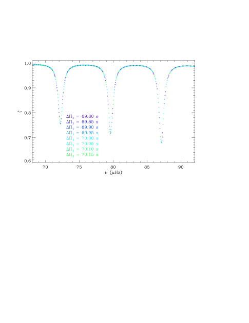
The functions $\zeta$ for close values of $\Delta\Pi_{1}$ are very similar, to those obtained for a typical RGB star (see Fig. 1). The pressure-mode parameters $\Delta\nu$ and $\nu_{\mathrm{max}}$ are fixed, whereas different values of $\zeta$ are shown for different values of $\Delta\Pi_{1}$. This property allows us to obtain a nearly continuous function $\zeta$, for the most precise use of Eq. (7), with small modifications of the period spacing around a given value of $\Delta\Pi_{1}$. For the most efficient computation of $\zeta$ for a given value of $\Delta\Pi_{1}$, variations in the range $\Delta\Pi_{1}(1\pm\nu_{\mathrm{max}}\Delta\Pi_{1}/2)$ have to be investigated (Fig. 1).

The minimum values of $\zeta$ are governed by the global seismic parameters describing the pressure mode pattern. At first order, these minimum values are located near the first-order frequencies of dipole pressure modes $(n_{\mathrm{p}}+\varepsilon_{\mathrm{p}}+d_{01})\Delta\nu$, where $\varepsilon_{\mathrm{p}}$ is the asymptotic offset for pressure modes and $d_{01}$ is the small separation for dipole modes. The large separation ($\Delta\nu$) determines the frequency difference between each minima of $\zeta$, and $\varepsilon_{\mathrm{p}}$ and $d_{01}$ define the position of the dipole pressure modes (e.g., Mosser et al. 2011b), and so determine the location of these minima. A change in these parameters can potentially produce an important change in $\zeta$. However, these parameters are precisely determined from the radial mode pattern and by the frequency shift $d_{01}$ depicted by the universal red giant oscillation pattern.

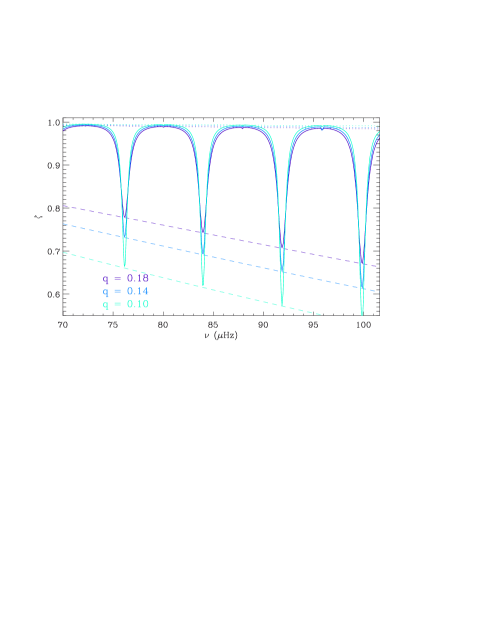
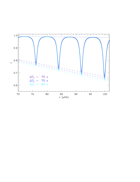
On the contrary, the function $\zeta$ hardly depends on $q$ and $\Delta\Pi_{1}$. As explained in Mosser et al. (2015), the coupling parameter $q$ determines the depth of the minima (Fig. 2top). Since this parameter does not vary much during the red giant evolution (Mosser et al. 2012c), it has little influence on $\zeta$. For the dependence of $\zeta$ with $\Delta\Pi_{1}$, the scaling of $\Delta P$ to $\Delta\Pi_{1}$ makes the function approximately the same for each $\Delta\Pi_{1}$. It follows that the values of $\Delta\Pi_{1}$ and $q$ have only a limited impact on $\zeta$ (Fig. 2middle).

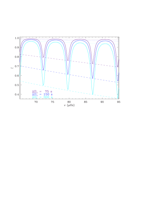
As a result, the determination of $\Delta\nu$ and of the frequency position of the dipole pressure modes is enough to provide a relevant estimate of $\zeta$. Therefore, using this function to stretch the oscillation spectra results in the emergence of a regularity corresponding to the $\Delta\Pi_{1}$ value. Even a large change in $\Delta\Pi_{1}$ does not modify $\zeta$ drastically (Fig. 2bottom), so that a RGB star can be treated with a clump $\Delta\Pi_{1}$ value to initiate the stretching, and conversely. This property is demonstrated in Appendix A.1.

3 Automated measurement of $\Delta\Pi_{1}$

In this section, we detail the way to measure period spacings in a fully automated way.

3.1 Preparation of the oscillation spectrum

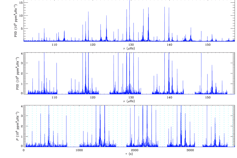
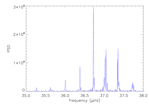
The first steps of the setup are based on the pressure modes. First estimates of the values of $\Delta\nu$ and $\nu_{\mathrm{max}}$ are obtained with the envelope autocorrelation function (Mosser & Appourchaux 2009). These values are refined by using the universal pattern (Mosser et al. 2011b) in order to enhance the accuracy of the determination of $\Delta\nu$ and to precisely locate the different oscillation modes. We do not include radial modes in our study since they do not exhibit mixed modes, or quadrupole mixed modes since they are confined near the pressure modes and do not exhibit the same pattern as dipole mixed modes. Therefore, we suppress these modes from the spectra (second panel of Fig. 3). In practice, this operation only depends on the value of the large separation: we keep part of the spectrum with a second-order reduced frequency $x_{\nu}$ verifying

$$x_{\nu}={\nu\over\Delta\nu}-\left(n_{\mathrm{p}}+\varepsilon_{\mathrm{p}}+{\alpha\over 2}(n-n_{\mathrm{max}})^{2}\right)\in[0.06,0.80],$$ (9)

where the quadratic term accounts for the second-order asymptotic expansion (Mosser et al. 2011b, 2013). In order to avoid discontinuities due to the granulation background, this operation is applied to a background-corrected spectrum (Fig. 3b). The background is determined as in Mosser et al. (2012a).

Figure 3: Top: Oscillation spectrum of the red giant KIC9145955 in function of frequency. Middle: Radial and quadrupole modes have been removed and the background has been subtracted from the spectrum. Bottom: Oscillation spectrum as a function of the stretched period. The light blue dashed lines correspond to a regular Dirac comb (indicated with dashed lines).

3.2 Initial values

In order to help the iterative process, we chose initial values of $\Delta\Pi_{1}$ that agree with the $\Delta\Pi_{1}$-$\Delta\nu$ pattern presented by Mosser et al. (2014). For $\Delta\nu$ above 9.5 $\mu$Hz, there is no ambiguity since the only possible evolutionary status is RGB. Below this value, stars may be on the RGB, in the clump, or leaving the clump. This last case is equivalent to the clump phase, since the $\Delta\Pi_{1}$ shows continuous variation at the end of the clump. So, different cases were then tested for $\Delta\nu$ below 9.5 $\mu$Hz, with a guess value agreeing either with the RGB or with the other evolutionary stages.

We then stretched the oscillation spectrum using the $\zeta$ function as described in section 2 (bottom panel of Fig. 3).

3.3 Spectrum of the stretched spectrum

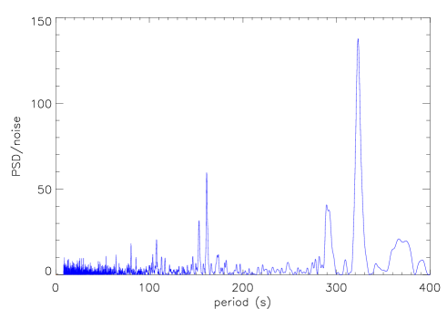
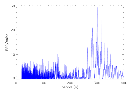
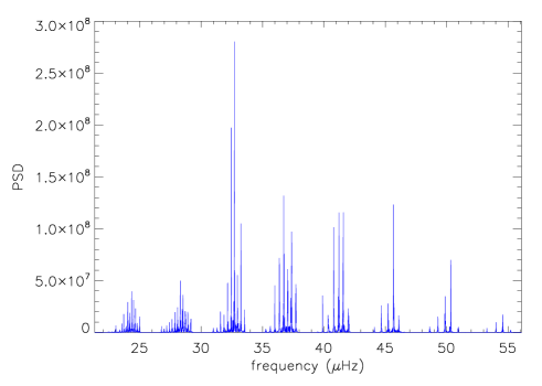
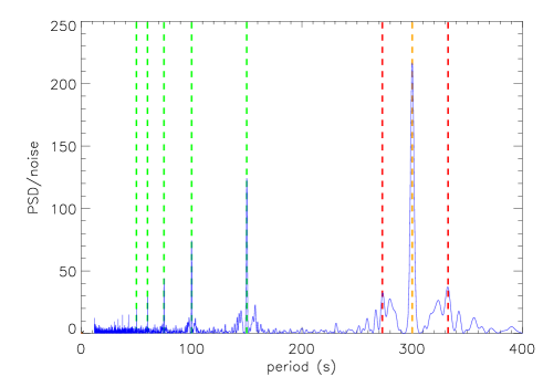
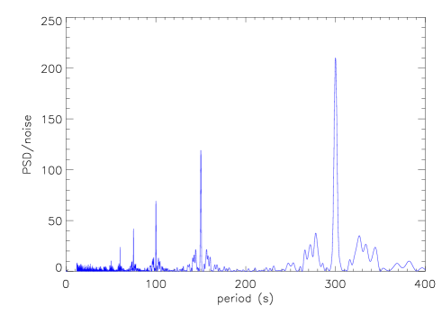
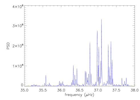
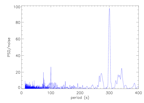
To retrieve the $\Delta\Pi_{1}$ value, we performed a Fourier transform of the new spectrum $\mathcal{P}(\tau)$ (Fig. 4). Owing to the form of the mixed-mode signal, with high amplitudes for the pressure-dominated mixed modes and low amplitudes for the gravity-dominated modes, there is no need to use a tapering function to smooth the spectrum and reduce aliases since the distribution of the amplitudes naturally mimics a tapering function.

Regularity in the stretched spectrum results in a clear signature in its Fourier spectrum (Fig. 4). As stated above, the period signature observed is largely independent of the initial guess value of $\Delta\Pi_{1}$ and $q$. However, a change in these initial values will produce a small variation in the measured period signature. An iterative process provides a stable measurement of the two parameters $q$ and $\Delta\Pi_{1}$ after only four steps (see Appendix A.1).

When necessary, we tested the different possible evolutionary stages and kept the coherent one: when the final value of $\Delta\Pi_{1}$ agrees with the hypothesis on the initial value. We also measured the mixed-mode period spacing $\Delta P$ and found very good agreement.

3.4 Test with a synthetic spectrum

In order to check possible bias of the method, we performed tests with synthetic low-degree oscillation spectra, using the asymptotic relations for the frequencies of radial and dipole mixed modes. Mode amplitudes were computed following Mosser et al. (2012a). The linewidths of the profile of the mixed modes, described as Lorentzians, were derived from observations. The linewidths of the radial and $\ell=2$ modes, useless for computing the period spacing but necessary for testing the whole automated chain, were computed following Belkacem et al. (2012). We finally multiplied the mixed-mode amplitudes with a Gaussian function to take into account the amplitude difference between pressure-dominated and gravity-dominated modes. The FWHM of this Gaussian was fixed to one-fifth of the large separation to match observed spectra. The result is shown in the top part of Fig. 5.

We tested different values of $\Delta\Pi_{1}$, $\nu_{\mathrm{max}}$ and $\Delta\nu$ and retrieved in each case the initial value of $\Delta\Pi_{1}$ with a precision much higher than 0.1 % (Fig. 5).

Figure 4: Top: Power spectrum of $P(\tau)$ as a function of the period for the star KIC 1995859. $\Delta\Pi_{1}$ for this star is 321 s. Middle: Same figure for KIC 1868101 with $\Delta\Pi_{1}=300.6$ s. Bottom: Same figure for KIC 12507577 with $\Delta\Pi_{1}=66.3$ s.

3.5 Performance and uncertainties

3.5.1 Confidence level

To define the confidence level, we measured the mean high-frequency noise present in the spectrum and used this value to normalize the Fourier spectrum $\mathcal{S}$ of the stretched spectrum $\mathcal{P}(\tau)$. In order to estimate the relevance of the detection, we assumed that the statistics of $\mathcal{S}$ follows a $\chi^{2}$ distribution. This is not strictly the case, owing to the rescaling from the frequency to the period domain and to the stretching of the spectrum induced by the change of variable (Eq. 7). However, these deformations are limited in the frequency range around $\nu_{\mathrm{max}}$ so that we use a similar test to the one provided by the H₀ hypothesis, but with a dedicated calibration.

Assuming a $\chi^{2}$ distribution, the detection can be considered reliable when the local maximum of $\mathcal{S}$ is larger than ten times the mean noise level; the detected value then corresponds to a period signature rejecting the $H_{0}$ hypothesis corresponding to pure noise with more than 99.9 % confidence (Mosser & Appourchaux 2009). Simulations, consisting in retrieving the oscillation signal in a high signal-to-noise spectrum corrupted with white noise, showed that the detection is relevant with the threshold level previously mentioned fixed at the value $13$.

Figure 5: Top: Simulated mixed-mode spectrum. Radial and $\ell=2$ modes are absent, as depicted in Figure 3. Bottom: Power spectrum of $P(\tau)$ derived from the asymptotic relation. The initial $\Delta\Pi_{1}$ value was settled at 300 s. The principal aliases observed around $\Delta\Pi_{1}$ are indicated by red dashed lines. Harmonics of $\Delta\Pi_{1}$ are also seen (green dashed lines).

Table 1: Estimates of the different uncertainties for a typical RGB star with $\Delta\nu=8\,\mu$Hz and $\nu_{\mathrm{max}}=75\,\mu$Hz or for a typical clump star with $\Delta\nu=4\,\mu$Hz and $\nu_{\mathrm{max}}=35\,\mu$Hz

	RGB		clump
$\Delta\Pi_{1}$ (s)	75		300
$\delta(\Delta\Pi_{1})_{\mathrm{res}}$ (s)	0.5		3.1
$\delta(\Delta\Pi_{1})_{\mathrm{order}}$ (s)	0.5		3.1
$\delta(\Delta\Pi_{1})_{\mathrm{alias}}$ (s)	5.1		27
$\mathrm{max}(\mathcal{S})$	15	30	15	30
$\delta(\Delta\Pi_{1})_{\mathrm{over}}$ (s)	0.05	0.02	0.34	0.17

3.5.2 Uncertainties

The precision that can be achieved for the measurement of $\Delta\Pi_{1}$ depends on the time resolution of the Fourier spectrum $\mathcal{S}$ of the stretched spectrum. This resolution, related to the properties of the oscillating signal, expresses as

$$\delta(\Delta\Pi_{1})_{\mathrm{res}}=\nu_{\mathrm{max}}\ \Delta\Pi_{1}^{2},$$ (10)

as derived in Appendix A.2. It then provides a quantitative basis for estimating reliable uncertainties.

We investigated three different cases, depending on the mixed-mode pattern density. If the mixed-mode pattern is dense with many gravity-dominated mixed modes, then the precision on the measurement is high since the function $\mathcal{S}$ can be oversampled (Fig. 4, top panel). It then writes, as a function of the nominal resolution $\delta(\Delta\Pi_{1})_{\mathrm{res}}$,

$$\delta(\Delta\Pi_{1})_{\mathrm{over}}\simeq{1.6\over A}\ \delta(\Delta\Pi_{1})_{\mathrm{res}},$$ (11)

where $A$ is the maximum value of $\mathcal{S}$ reached at $\Delta\Pi_{1}$.

However, the accuracy on $\Delta\Pi_{1}$ also depends on the constant $\varepsilon_{\mathrm{g}}$ of the asymptotic gravity modes. At this stage, there is no complete study on this parameter (see Provost & Berthomieu 1986, for a dedicated study), so that one cannot fix its value. An uncertainty of 1 in $\varepsilon_{\mathrm{g}}$ translates into an uncertainty of one radial gravity order. As shown in Appendix A.4, the uncertainty is then

$$\delta(\Delta\Pi_{1})_{\mathrm{order}}=\delta(\Delta\Pi_{1})_{\mathrm{res}}.$$ (12)

This means that the high statistical precision has to be tempered by our inability to determine the value of the offset $\varepsilon_{\mathrm{g}}$. When only a low number of gravity dominated mixed-modes are observed, it is not possible to unambiguously measure $\Delta\Pi_{1}$ (second panel of Fig. 4). In this case, the uncertainty corresponds to a shift of one radial order.

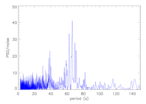
For evolved RGB stars, gravity-dominated mixed modes have inertia that is too high, which means that they cannot be observed (Grosjean et al. 2014). In such cases, the ambiguity for measuring $\Delta\Pi_{1}$ corresponds to a window effect. The absence of observable mixed modes in the frequency ranges close to quadrupole and radial modes yields large uncertainties. Instead, the observation of a few mixed modes in this region is most often enough to remove any degeneracy in the solution. As explained in Appendix A.5, the frequency shift due to missing gravity-dominated mixed modes around radial and quadrupole modes is

$$\delta(\Delta\Pi_{1})_{\mathrm{alias}}\simeq n_{\mathrm{max}}\ \delta(\Delta\Pi_{1})_{\mathrm{order}},$$ (13)

and helps estimate the large uncertainty introduced by an alias mismatch. For red giants, values of $n_{\mathrm{max}}$ are typically about ten. Typical values of the uncertainties are given in Table 1.

4 Comparison with previous results

To test the efficiency of the method, we compared the results obtained to the 1110 stars where Mosser et al. (2014) have manually measured the parameter $\Delta\Pi_{1}$. We excluded subgiants and early red giants that have a large separation $\Delta\nu$ larger than 18 $\mu$Hz from their original data set. The oscillation spectrum of these stars can be retrieved in short-cadence time series only and are out of reach of the long-cadence data used here.

Figure 6: $\Delta\Pi_{1}$ (s) in function of the large separation $\Delta\nu$ ($\mu$Hz) for the set of stars analyzed by Mosser et al. (2014). The uncertainties correspond to the 1-$\sigma$ error bars.

We were able to deduce the $\Delta\Pi_{1}$ for more than 600 stars (Fig. 6). The results show a good agreement between the $\Delta\Pi_{1}$ measured either manually or automatically as shown in Fig. 7, since the relative difference is less than 2 % for more than 80 % of the stars, and less than 10 % for more than 90 % of the stars. In fact, the bump present at $-$10 % and $+$10 % corresponds to the window effect described in Section 3.5. We confirmed that a confusion between the different evolutionary states is very rare. We found only two cases in this sample where this situation was observed.

Figure 7: Histogram of the relative differences between the values $\Delta\Pi_{1}$ obtained automatically or individually.

We note, however that the automated method fails to retrieve a $\Delta\Pi_{1}$ estimate in three main cases:
- Measuring $\Delta\Pi_{1}$ is difficult at low $\Delta\nu$ when the number of gravity-dominated mixed modes is small (Dupret et al. 2009; Grosjean et al. 2014) and when the frequency resolution is poorer than the frequency difference between consecutive mixed modes. This is particularly true for evolved RGB stars or AGB stars.
- When mixed modes have a low visibility (Mosser et al. 2012a; García et al. 2014), only the manual inspection of such stars can provide $\Delta\Pi_{1}$, under the condition that the mode visibility is not too small.
- In a limited number of cases, buoyancy glitches that induce a modulation of the period spacing are large enough to hamper the measurement of the mean period spacing with a Fourier analysis. Often, the modulation is small and the method works, but may deliver preferably an alias of $\Delta\Pi_{1}$. We leave the analysis of glitches to a forthcoming work.

On the contrary, we noted that the presence of rotational splitting does not affect the determination of the $\Delta\Pi_{1}$ value because the $\zeta$ function is efficient at straightening the mixed-mode pattern even when split by rotation. Each azimuthal order $m$ forms a family with evenly spaced stretch periods, with a spacing ${\Delta\Pi_{1}}_{,m}$ given by Mosser et al. (2015)

$${\Delta\Pi_{1}}_{,m}\simeq\Delta\Pi_{1}\ \left(1+2m{\mathcal{N}\over\mathcal{N}+1}\,{\delta\nu_{\mathrm{rot}}\over\nu_{\mathrm{max}}}\right),$$ (14)

where $\mathcal{N}$ (equal to $\Delta\nu/\Delta\Pi_{1}\nu_{\mathrm{max}}^{2}$) represents the number of gravity modes in the $\Delta\nu$-wide frequency range around $\nu_{\mathrm{max}}$, and where $\delta\nu_{\mathrm{rot}}$ is the maximum rotational splitting. These rotational splittings are small compared to the frequency $\nu_{\mathrm{max}}$, so that the correction proportional to the azimuthal order $m$ is in fact smaller than the resolution $\delta(\Delta\Pi_{1})_{\mathrm{res}}$ (Eq. 10). As a consequence, the period spacings of all components of the dipole modes are close to $\Delta\Pi_{1}$, and rotation is not an issue for measuring $\Delta\Pi_{1}$.

Figure 8: Left: zoom on a precise radial order of the simulated mixed-mode spectrum shown in Figure 5. $\chi^{2}$ noise with two degrees of freedom has been included in the spectrum with an height corresponding to $1/50$ of the height of the oscillations. Right: Power spectrum of $P(\tau)$ derived from the simulated spectra. Top: simulations without rotation. Bottom: same simulations but with the addition of rotational splittings, which appear as rotational triplets with a $\delta\nu_{\mathrm{rot}}$ equal to $0.054$ $\mu$Hz.

In order to highlight these statements, we constructed several synthetic spectrum as described in Section 3.4 with the addition of rotational splittings obtained from Eq. (17) of Deheuvels et al. (2015). We considered the case of a star seen with an inclination angle of 45^∘ and a star seen equator-on corresponding respectively to the observation of rotational triplets and rotational doublets. In each case, the splitting amplitudes are considered equal. An example of a part of the synthetic spectrum is shown on the left side of Fig. 8. The power spectra of $P(\tau)$ derived from the synthetic spectra, where rotational triplets were included, are shown on the right side of Fig. 8. Different values of $\Delta\Pi_{1}$ and $\delta\nu_{\mathrm{rot}}$ have been tested. In each case, the initial $\Delta\Pi_{1}$ value has been retrieved with a precision higher than $0.2$ $\%$. The only visible signature of rotation is an apparent decrease in the power spectrum of $P(\tau)$.

5 Treatment of Kepler red giant public data

5.1 Data

Figure 9: $\Delta\Pi_{1}$ in function of the large separation $\Delta\nu$ for the Kepler red giant public data. The color code indicates the stellar mass ($M_{\odot}$) The signatures of the RGB, the main clump and the secondary clump appear clearly. The proportion of outliers, compared to the seismic evolutionary tracks defined in Mosser et al. (2014), is less than 1 %.

We used the public long-cadence data from Kepler with the maximum available length, up to the quarter Q17, corresponding to 44 months of photometric observation. Original light curves were taken from the MAST program (Fanelli et al. 2011; Fraquelli & Thompson 2014). Among the 15 000 light curves in the Kepler public data, we processed the set of more than 12900 stars for which the large separation $\Delta\nu$ can be reliably measured.

5.2 Gravity period spacing

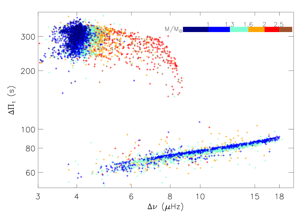
We were able to determine $\Delta\Pi_{1}$ for about 6 100 red giants. The other stars did not satisfy the reliability level defined in Section 3.5.1 owing to a low signal-to-noise ratio in the spectra or to the presence of too few g-dominated mixed modes. In some limited cases, it was due to an incorrect identification of the radial mode pattern. Despite the various checks, there are about 45 outliers in Figure 9; they represent less than 1 % of the total of the detections. We note, however, that large uncertainties due to the alias problem affect about 20 % of the values, especially on the RGB at low $\Delta\nu$. The data, obtained with two different codes, are available at the CDS (Table 2)

Table 2: Global seismic parameters

KIC number	$\Delta\nu$ ($\mu$Hz)	$\Delta\Pi_{1}$ (s)	$\delta\Delta\Pi_{1}$ (s)	$q$	$M/M_{\odot}$	$\delta M/M_{\odot}$	alias	method	evolution
1868101	3.80	298.7	2.80	0.35	0.93	0.05	0	2	1
1995859	4.74	321.4	4.71	0.29	1.86	0.06	0	2	1
9145955	11.03	77.1	1.50	0.16	1.44	0.06	0	1	0
12507577	7.52	69.7	0.40	0.21	1.45	0.06	0	2	0

Global seismic parameters, as described in the text, of the four stars shown in Figs. 3 and 4. The full table corresponding to the whole data set shown in Fig. 9, with about 6 100 red giants, is available at CDS via anonymous ftp to cdsarc.u-strasbg.fr (130.79.128.5) or via http://cdsarc.u-strasbg.fr/viz-bin/qcat?J/A+A/NNN/PPP”. Uncertainties on $\Delta\Pi_{1}$ are estimated according to the expressions given in the Appendix. They depend on the robustness of the measurement, which is indicated in the columns ’alias’and ’method’ The ’alias’ value is set to 1 if the value of $\Delta\Pi_{1}$ likely corresponds to that of an alias, otherwise to 0. The ’method’ value indicates whether 1 or 2 codes using the method presented in the article could converge and provide a relevant value for $\Delta\Pi_{1}$; a value of 2 also means that both codes provide consistent results. The ’evolution’ value provides the evolutionary stage: 0 for RGB stars, 1 for clump stars, or 2 for secondary clump stars.

The results confirm and extend the conclusions of (Bedding et al. 2011; Mosser et al. 2012c; Stello et al. 2013; Mosser et al. 2014), taking into account that here we measure asymptotic values and not mean period spacings. We see the same characteristic features except for stars starting the ascension of the AGB identified by Mosser et al. (2014). Their absence can be explained by the low signal-to-noise ratio of oscillation spectra at low $\Delta\nu$, which then induces the rejection of the measurements; instead, such stars can be analyzed individually.

Table 3: Values of the period spacings $\Delta\Pi_{1}(M,Z)$, in seconds, for a large separation $\Delta\nu=6\,\mu$Hz, with the scaling relation $\Delta\Pi_{1}\propto\Delta\nu^{0.25}$. Uncertainties are of about 0.25 s.

$M/M_{\odot}$	1.0-1.2	1.2-1.4	1.4-1.6
$Z<-0.4$	68.0	67.9	67.3
$-0.4<Z<0$	68.7	68.2	67.4
$Z>0$	69.1	68.5	67.5

5.3 Mass and metallicity

Figure 10: $\Delta\Pi_{1}$ (s) in function of the large separation $\Delta\nu$ ($\mu$Hz) for the Kepler red giant public data. The color code indicates the stellar mass ($M_{\odot}$). We have superimposed two curves indicating the regions where aliases are expected. We note the large number of such artefacts below 9 $\mu$Hz.

Figure 11: Fit of the $\Delta\Pi_{1}$ – $\Delta\nu$ relation depending on the stellar mass and metallicity.

Figure 12: Same as Fig. 9, with red giants identified as members of three open clusters observed by Kepler: NGC 6791, triangles; NGC 6819, diamonds; NGC 6811, squares.

The scaling relations allow the determination of the stellar masses and radii from the global seismic parameters ($\Delta\nu$, $\nu_{\mathrm{max}}$) and from the effective temperature (e.g., Kallinger et al. 2010). We used the effective temperature listed in Huber et al. (2014). The relative uncertainties on the stellar mass are about 10-15$\%$. The variations of $\Delta\Pi_{1}$ along the stellar evolution for different star masses can then be analyzed.

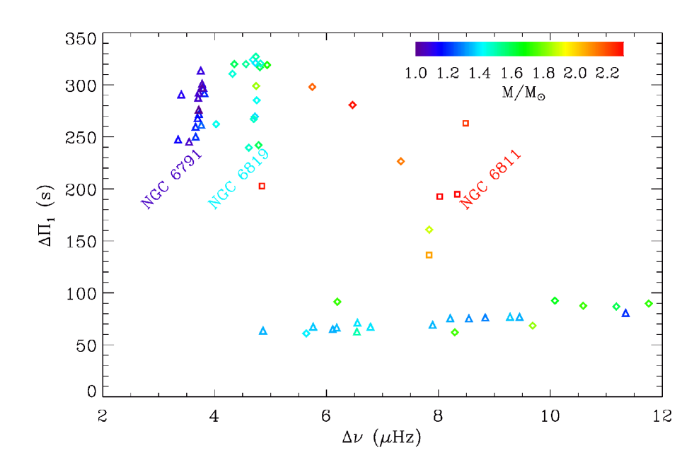
The mass dependence present in the main and secondary clumps (e.g., Bedding et al. 2011; Mosser et al. 2014) is confirmed. This is illustrated in Fig. 12 with a subsample of Fig. 9, with stars from the open clusters NGC 6791 ($M_{\mathrm{6791}}=1.15\pm 0.03\,M_{\odot}$ in the RGB), NGC 6811 ($M_{\mathrm{6811}}=2.2\pm 0.1\,M_{\odot}$), and NGC 6819 ($M_{\mathrm{6811}}=1.61\pm 0.04\,M_{\odot}$). The membership of these stars is defined as in Stello et al. (2010); the masses are derived from Miglio et al. (2012). The evolutionary tracks of the three clusters are close to each other on the RGB, where the mass dependence is weak, but important in the helium-burning phase. We confirm the identification of three blue stragglers in NGC 6819, already identified by Corsaro et al. (2012).

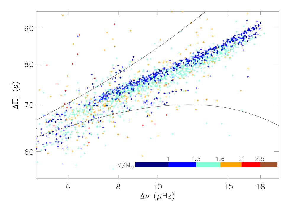
We also discovered another mass dependence present in the RGB branch. At fixed properties of the stellar core (at fixed $\Delta\Pi_{1}$), a high-mass RGB star has a larger $\Delta\nu$ value than a low-mass star. This means that, despite a more massive convective envelope, high-mass stars are more dense. This relation, observed for RGB stars with a mass below 1.6 $M_{\odot}$, is predicted by simulations (Stello et al. 2013), but has never been observed. We also note that stars on the RGB with a mass above 1.6 $M_{\odot}$ exhibit a large spread around the RGB branch. This phenomenon, already noted by Mosser et al. (2014), can be related to the different physical conditions when such stars reach the RGB.

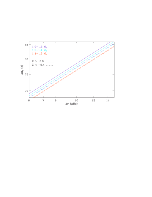
The large number of stars on the RGB with a precise measurement of $\Delta\Pi_{1}$ also allowed us to test the metallicity dependence of the $\Delta\Pi_{1}$ – $\Delta\nu$ relation. At fixed properties of the core (at fixed $\Delta\Pi_{1}$), we observe that low metallicity stars have a large spacing $\Delta\nu$ significantly higher than most metallic stars (Fig. 11). The values of $\Delta\Pi_{1}(M,Z)$ for $\Delta\nu=6\,\mu$Hz are given in Table 3. Uncertainties on these values are about 0.25 s, significantly less than the observed spread. The metallic dependance is high for stars below 1.2 $M_{\odot}$, but negligible for stars above 1.4 $M_{\odot}$. This agrees with the fact that low-metallicity stars are denser. The fits in Fig. 11 were obtained assuming that the slope of the $\log(\Delta\Pi_{1})$ – $\log(\Delta\nu)$ relation is fixed, equal to 0.25 according to the global fit.

5.4 Luminosity bump

We also note the large spread on the $\Delta\Pi_{1}$ value for RGB stars with $\Delta\nu$ lower than $6.5$ $\mu$Hz. This spread occurs where simulations predict the position of the luminosity bump (Lagarde et al. 2012). The spread could then be due to such a phenomenon.

The aliasing phenomenon complicates the result at low $\Delta\nu$ on the RGB and precludes the firm identification of the signature of the luminosity bump, as discussed above. The main aliases are present as the second branch observed under the RGB branch.

Figure 13: Histogram of the coupling factor $q$. The dashed blue line corresponds to RGB stars and the continuous red line to clump stars.

5.5 Coupling parameter

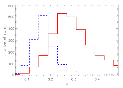
The coupling factor $q$ was adjusted along with $\Delta\Pi_{1}$. The results are shown in Fig. 13.

Red giant branch stars show a smaller coupling than clump stars, as stated by Mosser et al. (2012c). Our results are similar to this study for RGB stars: the mean value is $q=0.17\pm 0.05$. However, the results for clump stars are higher: around $0.29\pm 0.07$, but still in the previously estimated uncertainties. The clump stars present a stronger coupling between p and g modes than RGB stars.

Following Unno et al. (1989), the value of the coupling factor is linked to the extent of the evanescent region and is limited to 1/4. Our results, however, do not verify this: we measure $q$ values significantly above 1/4. This discrepancy arises because the formalism in Unno et al. (1989) is only valid for a weak coupling (M. Takata, private communication), which is not observed. A new development is necessary to link $q$ and the size of the evanescent zone, as stated by Jiang & Christensen-Dalsgaard (2014).

6 Conclusion

We presented a new method based on the inversion of the mixed-mode asymptotic relation for determining automatically the gravity period spacing in the mixed-mode pattern of red giants stars. The efficiency of the method derives from the asymptotic properties of the radial and dipole spectrum: the radial oscillation pattern follows the universal red giant oscillation pattern, which corresponds to a second-order asymptotic development; the dipole oscillation pattern is tightly fitted by the asymptotic expansion for mixed modes. The change of variable used to analyze the stretched periods of the modes allows us to exhibit the properties of the oscillation periods and not of period spacings.

We used this new method on the red giant Kepler public data and succeeded in deducing the gravity period spacing for about 6 100 red giants. The results obtained confirmed previous measurement for these stars. We unveil as well a new mass dependence for RGB stars: higher-mass stars will have a lower period spacing. This work paves the way to the precise interpretation of the mixed-mode pattern on numerous stars; a massive measurement of rotational splittings is now possible. We note that buoyancy glitches sometimes hamper the detection of $\Delta\Pi_{1}$, but such glitches deserve a specific study.

Appendix A Uncertainty on $\Delta\Pi_{1}$

The measurement of $\Delta\Pi_{1}$ depends on the characteristics of the stretched spectrum and of its spectrum. We first examine how they are connected with the method and with the global seismic properties of the spectrum. The exact measurement of $\Delta\Pi_{1}$ presupposes as well the exact determination of the mixed-mode order, which depends on the value of the gravity offset $\varepsilon_{\mathrm{g}}$. The measurement is also perturbed by the low amplitudes of gravity-dominated mixed modes. Since these modes are evenly spaced in frequency, this effect is comparable to a window effect. All these effects are examined.

A.1 Uncertainties of the stretching process

The accuracy of the stretching process is ensured by the principle of the method and the use of Eq. (7). In this equation, the difference between periods and stretched periods is due to the term $1/\zeta$, which basically ensure that there are $\mathcal{N}+1$ modes in a $\Delta\nu$-wide interval, where $\mathcal{N}=\Delta\nu/\Delta\Pi_{1}\nu^{2}$ modes are expected. As a result, the relative difference between periods and stretched periods is measured by $1/\mathcal{N}$. Except for subgiants and on the early RGB where $\mathcal{N}$ has small values (Mosser et al. 2014), the large values of $\mathcal{N}$ for the RGB and clump stars considered in this work ensures an efficient iteration. In order to illustrate this, Table 4 shows the convergence of the iteration process in the case of an RGB star with $\Delta\Pi_{1}=75$ s, with two initial guess values (RGB or clump). Even if the initial guess value corresponds to an incorrect determination of the evolutionary stage, the iteration process precisely converges after four steps.

A.2 Resolution of the spectrum of the stretched spectrum

We examine the properties of the stretched spectrum and of its spectrum.

Since the frequency range where modes are observed is typically $\nu_{\mathrm{max}}$, the period range of the stretched spectrum is about $1/\nu_{\mathrm{max}}$. Then, the spectrum of this spectrum typically has a resolution $\nu_{\mathrm{max}}$. Since the signature of the period spacing $\Delta\Pi_{1}$ occurs at $1/\Delta\Pi_{1}$, the nominal resolution expressed in the period variable is

$$\delta(\Delta\Pi_{1})_{\mathrm{res}}=\nu_{\mathrm{max}}\Delta\Pi_{1}^{2}.$$ (15)

Typical values of the nominal resolution correspond to about 0.4 s on the RGB and 3.6 s in the red clump.

A.3 Uncertainties with an oversampled spectrum

The high quality of signal allows us to oversample the spectrum in order to increase the resolution. This tighter resolution is, however, limited by the noise. Following the same approach as in Mosser & Appourchaux (2009), and especially their equations (A.4)-(A.6), we can compare the variation of the signal peaking at amplitude $A$ to the maximum variation of a noise contribution of amplitude $b$ (both expressed in white noise units). The precise identification of the signal maximum allows us to compare the oversampled resolution $\delta(\Delta\Pi_{1})_{\mathrm{over}}$ to the nominal resolution

$$\pi A\ \delta(\Delta\Pi_{1})_{\mathrm{over}}\geq b\ \delta(\Delta\Pi_{1})_{\mathrm{res}}.$$ (16)

Considering a conservative value $b=5$, in white noise units, we have

$$\delta(\Delta\Pi_{1})_{\mathrm{over}}\simeq{1.6\over A}\ \delta(\Delta\Pi_{1})_{\mathrm{res}}.$$ (17)

Values of $A$ above the threshold level ensure a significantly tighter resolution than the nominal value $\delta(\Delta\Pi_{1})_{\mathrm{res}}$. Since $A$ may be as high as 200, the accuracy of the measurement may become excellent; however, this supposes that the gravity offset $\varepsilon_{\mathrm{g}}$ intervening in the pure gravity-mode pattern is known. It is usually set to 0, although the asymptotic value is 1/4 (Tassoul 1980). Anyway, its expression can be complicate, depending on the structure of the radiative core (Provost & Berthomieu 1986).

A.4 Uncertainties corresponding to a shift of one gravity order

According to the asymptotic theory, the gravity mode periods are evenly spaced with a mean period spacing close to $\Delta\Pi_{1}$. So, their frequencies express

$$\nu=\frac{1}{n_{\mathrm{g}}\Delta\Pi_{1}},$$ (18)

where $n_{\mathrm{g}}$ is the gravity order. By deriving this equation, we obtain

$$\frac{\mathrm{d}\nu}{\nu}=-\frac{\mathrm{d}n_{\mathrm{g}}}{n_{\mathrm{g}}}-\frac{\mathrm{d}\Delta\Pi_{1}}{\Delta\Pi_{1}}.$$ (19)

A shift of one radial order corresponds to $\mathrm{d}n_{\mathrm{g}}=1$. For a fixed set of oscillation modes, we have $\mathrm{d}\nu=0$. It follows that $\mathrm{d}\Delta\Pi_{1}=\Delta\Pi_{1}/n_{\mathrm{g}}$. By assuming that we are near the maximum oscillation frequency $\nu_{\mathrm{max}}$ and following Eq. (18), the error on $\Delta\Pi_{1}$ can be written as

$$\delta(\Delta\Pi_{1})_{\mathrm{order}}=\nu_{\mathrm{max}}\Delta\Pi_{1}^{2}.$$ (20)

So we note that we obtain a similar result to that determined by the resolution:

$$\delta(\Delta\Pi_{1})_{\mathrm{order}}=\delta(\Delta\Pi_{1})_{\mathrm{res}}.$$ (21)

A.5 Uncertainties corresponding to the window effect

The suppression of the radial and quadrupole modes we performed possibly leads to what is called a window effect. The removal of part of the spectrum at regular frequencies produces aliases (equal to $1/\Delta\nu$ in period), which could be mistakenly attributed to the real value of $\Delta\Pi_{1}$. To estimate the uncertainties related to this possible confusion, we also have to estimate the frequency difference between each mode. To this end, we follow Eq. (19) with a fixed $\Delta\Pi_{1}$ value ($\mathrm{d}\Delta\Pi_{1}=0$) and an order variation $\mathrm{d}n_{\mathrm{g}}=1$:

$$\frac{\mathrm{d}\nu}{\nu}=-\frac{1}{n_{\mathrm{g}}}.$$ (22)

With $n_{\mathrm{g}}$ determined by Eq. (18), the value of $\mathrm{d}\nu$ is equal to $\Delta\Pi_{1}\nu^{2}$. It corresponds to a signature at the period $1/(\Delta\Pi_{1}\nu^{2})$. The relative period shifts due to the aliases are then determined by

$$\frac{\mathrm{d}\Delta\Pi_{1}}{\Delta\Pi_{1}}={\displaystyle{1\over\Delta\nu}\over\displaystyle{1\over{\Delta\Pi_{1}\nu^{2}}}}.$$ (23)

For frequencies close to the maximum oscillation frequency $\nu_{\mathrm{max}}$, this shift translates into an uncertainty on $\Delta\Pi_{1}$ expressed by

$$\delta(\Delta\Pi_{1})_{\mathrm{alias}}=\frac{(\nu_{\mathrm{max}}\Delta\Pi_{1})^{2}}{\Delta\nu}.$$ (24)

This, however, relies on the detection of pure gravity modes. Here, mixed modes with stretched periods behave as gravity modes, but with an additional mode that is the pressure mode. Hence, the correct uncertainty is reduced by a factor $\mathcal{N}/(\mathcal{N}+1)$ so that

$$\delta(\Delta\Pi_{1})_{\mathrm{alias}}={(\nu_{\mathrm{max}}\Delta\Pi_{1})^{2}\over\Delta\nu}{\mathcal{N}\over\mathcal{N}+1}={\Delta\Pi_{1}\over\mathcal{N}+1}.$$ (25)

Table 4: Iteration process

Iteration step $i$	${\Delta\Pi_{1}}_{i}$ (s)
start value	80	300
1	75.30	88.50
2	75.018	75.810
3	75.0011	75.0486
4	75.0001	75.0029
target value	75	75