Weak Classicality in Coupled $N$-Level Quantum Systems

Abstract

The notion of ‘weak classical limit’ for coupled $N-$level quantum systems as $N\rightarrow\infty$ is introduced to understand the precise sense in which one attains classicality. There exist proofs that a system becomes classical at large $N$ Yaffe82 ; Ghir86 . On the other hand, it is known that non-locality and entanglement, the two hallmarks of non-classicality, thrive even as $N\rightarrow\infty$. We reconcile these results in this paper by showing that so called classicality is not so much an inherent property of the system, as it is a consequence of limited experimental resources. Our focus is largely on non-locality, for which we study the Bell-CHSH and CGLMP inequalities for $N$-level systems.

PACS numbers

03.67.-a, 03.65.Ud, 03.65.Ta

I Introduction

The behaviour of quantum systems in the so called large $N$ limit, where $N$ denotes the dimension of the Hilbert space for some degree of freedom, holds an abiding interest. This is in view of the proofs that a system becomes classical Yaffe82 ; Ghir86 as $N\rightarrow\infty$. In the context of spin, e.g., these proofs exploit an essential property of spin coherent states. Though spin coherent states are over complete at any finite value of $N$, they become orthonormal as $N\rightarrow\infty$, making them isomorphic to the classical phase space. This delicate limit has received renewed interest in studies on non-locality and entanglement in higher dimensional bipartite systems Merm80 ; Peres92 ; Arde91 ; Arde92 ; Kasz00 . Contrary to earlier expectations Merm80 , it was realised that non-locality and entanglement continue to thrive even as $N\rightarrow\infty$ Peres92 ; Arde91 ; Arde92 ; Kasz00 . These results also hold for the more recently proposed inequalities for testing non-locality in higher dimensional systems Kasz00 ; Coll02 ; FuLi04 . A reconciliation between the theorem mentioned above and these results is in order, if only for the sake of avoiding inconsistent interpretations. We show that this can be accomplished through the notion of weak classicality, for which we consider a coupled system of two $N$-level systems. Thereby this paper also serves a pedagogic purpose.

The paper is organised as follows. As the simplest nontrivial subgroup of $SU(N)$, $SU(2)$ embodies the idea of moments of observables in the $N$-level system. This is because the generators of $SU(N)$ can be constructed from the generators of $SU(2)$ and their higher order tensor moments. We thus demonstrate that observables that yield experimental signatures for both non-locality and entanglement necessarily involve contributions from the highest order tensor moments (Section II). In this context, an $N\times N$ system is equivalent to a spin $s\times s$ system, and we take $N=2s+1$. To substantiate the qualitative observations, we perform quantitative analyses involving (i) polynomial observables in spin operators (Section IV) , and (ii) projective measurements, which are easily related to actual experimental set-ups (Section V). We proceed to show that the so-called classical limit emerges when there are limited experimental resources, causing an inability to measure high order moments, and that it is not an inherent property of the system itself. In view of the well known results obtained in Brau92 ; Pope92 , we study the cases of entanglement and non-locality separately.

II Weak classical limit: algebraic analysis

II.1 Non-locality and the weak classical limit

A physical system is said to be governed by classical laws if it can be modelled by a theory of local hidden variables BellInequalities ; CHSHOrig . A violation of the Bell-CHSH inequality is a sufficient, but not necessary signal of the non-locality of a state (see Brun14 and references cited therein).

The family of states that violate the Bell-CHSH inequality includes pure as well as mixed states, with $N=2$ being the only exception. In fact, pseudo-Bell states, belonging to all $2\times 2$ subspaces of $N\times N$ systems, violate the Bell-CHSH maximally, even though their relative entanglement with respect to the fully entangled state can be negligible. Furthermore, incoherent sums of the pseudo-Bell states belonging to orthogonal subspaces also exhibit maximal violation, even if they are highly mixed Brau92 ; Pope92 .

Let the basis states in the respective Hilbert spaces of the two subsystems be labelled by $m_{i},~{}\mu_{j}=-s,-(s-1),\cdots,s-1,s$, in the conventional spin basis. The first example that is of interest to us is the pseudo two qubit subspace spanned by $\{\left|m_{i}\right\rangle,\left|m_{j}\right\rangle;\left|\mu_{k}\right\rangle,\left|\mu_{l}\right\rangle\}$ for some fixed values of the subscripts. The subspace supports states that violate Bell-CHSH inequality maximally, which are further related to each other by local transformations in the subspace. The observables that reveal non-locality are simply the Pauli operators in the subspaces.

Simple though this theoretical construction is, isolation of states in two-dimensional subspaces is nontrivial experimentally, requiring effective hamiltonians that operate almost entirely in the subspace. Generically, spin observables span the full space, and measuring mean values and their first few moments is easier, and more feasible. To see this, consider a Pauli operator, say

$$A=|m_{i}\rangle\langle m_{j}|+|m_{j}\rangle\langle m_{i}|$$ (1)

defined for the first subsystem. We wish to determine the overlap, $Tr[AT^{k}_{q}(\vec{S})]$, of $A$ with the irreducible tensor operators $T^{k}_{q}(\vec{S})$, defined by

$$T^{k}_{q}(\vec{S})=C_{k}(\vec{S}\cdot\vec{\nabla})^{k}r^{k}Y_{k,q}(\theta,~{}\phi)$$ (2)

where $\vec{S}$ is the spin operator, and Y${}_{k,q}(\theta,~{}\phi)$, are the spherical harmonics. The constant $C_{k}$ is free, and is usually fixed by setting the matrix elements to be

$$\langle m_{2}|T^{k}_{q}(\vec{S})|m_{1}\rangle=C(sks;m_{1}qm_{2})\sqrt{2k+1}$$ (3)

in terms of the Clebsch-Gordan coefficients. The tensor of rank $k$ yields moments of order $k$, of the spin operators, with $0\leq k\leq 2s$. By Wigner-Eckart theorem, the overlap of the Pauli operator $A$ with $T_{q}^{k}$ thrives even as $k\rightarrow 2s$ so long as $q=\pm|m_{i}-m_{j}|$, and therefore measurements of lower order tensors would not yield the correct expectation value of $A$, rendering the verification of the Bell inequality suspect.

This is essentially the crux of the argument. Determination of correlations involving direct products of such Pauli operators entails measurements of correlations involving tensor correlations of all orders, which would involve varied experimental techniques. Thus, if one has the wherewithal to measure moments only upto a rank $k<<2s$, it would well nigh be impossible to decide if a state with a spin $s$ is non-local.

II.2 Entanglement and the weak classical limit

Entanglement and Bell-CHSH non-locality are relative monotones only for pure two-qubit states. We now argue, qualitatively, how weak classicality works with higher dimensional entanglement. For that, it is sufficient to consider a pure state for an $N\times N$ system.

The condition for pure state entanglement is that either of the reduced states have nonzero entropy. In particular, the reduced states of a fully entangled state are completely mixed. A verification of this entails complete tomography, which, again, necessarily involves ascertaining that all the moments, including the highest order $k=N-1$, vanish Niel11 .

On the other hand, if the state is separable, the state of the subsystem is pure. A verification of purity again requires the measurement of $t^{2s}_{q}$, that is, the tensor components. A spin $s$ state has the resolution

$$\rho=\frac{1}{N}\Big{\{}1+\sum_{k=1}^{2s}\sum_{q=-k}^{k}(-1)^{q}t_{-q}^{k}T_{q}^{k}(\vec{S})\Big{\}},$$ (4)

and it is known that a pure state is determined, except for residual discrete ambiguities, by the tensor components $t^{2s}_{q}$ Ravi86 ; Ravi87 .

In short, even with ideal measurements, quantumness may not be revealed if the experimental resources are limited in the sense described above. This conclusion complements other results on classical limits that invoke decoherence Zure91 ; Brune96 ; Zure03 or coarse grained measurements Kofl07 , and of the experimental resolution of adjacent states in a Stern-Gerlach set-up Peres92 . In all these cases, the classical limit is not seen as an inherent property of the system, but as arising from extraneous exigencies, either because of environment, or precision, or lack of resources. Any of them may mask the quantumness of the state.

We now buttress the qualitative arguments by two quantitative analyses that focus on non-locality. We show that, generally, violations of the Bell-CHSH inequality improves, as the observables have terms that are of increasingly higher orders in spin operators. Almost invariably, these observables have supports in proper subspaces of the $N$-dimensional Hilbert space. As mentioned, the Bell-CHSH inequality is violated maximally when the support is two-dimensional. Keeping this in mind, we consider, 1) observables that are polynomial in $SU(2)$ generators and 2) observables based on projective measurements. Before we delve into either of the two analyses, we address the experimental setting.

III Quantitative analysis: the setting

For our purposes, it is sufficient to consider the completely entangled state (invariant under global $SU(N)$),

$$|0_{s}>=\frac{1}{\sqrt{2s+1}}\sum_{m=-s}^{s}(-1)^{m+s}|m,-m>.$$ (5)

To check the robustness of the results, we employ the CGLMP formulation Coll02 , as well as the Bell-CHSH functions arising from a large family of correlations. Note that CGLMP yields non-locality criterion that is dimension dependent. We do not discuss violations coming from proper subspaces since they have essentially been considered in the previous section.

Consider, first, the Bell-CHSH function

$$\mathcal{B}\equiv|\mathcal{C}(a,b)-\mathcal{C}(a,b^{\prime})|+|\mathcal{C}(a^{\prime},b)+\mathcal{C}(a^{\prime},b^{\prime})|,$$ (6)

which signals non-locality whenever $2<{\cal B}\leq 2\sqrt{2}$. Furthermore, we employ the standard detector configuration geometry defined by

$$\theta_{ab}=\theta_{a^{\prime}b}=\theta_{a^{\prime}b^{\prime}}=\frac{\theta_{ab^{\prime}}}{3},$$ (7)

The precise meaning of $\theta$ will become clear from the examples discussed below. This prescription is not ad hoc for two reasons. An extensive study, partly analytical and partly numerical has shown this geometry to be optimal Mend05 . Our own computation confirms that maximal violations occur at this geometry for higher spins as well. The parameter space is thus rendered one dimensional.

IV Observables that are polynomial in $SU(2)$ generators

Our quantitative studies begin with correlations arising from polynomial observables in spin operators of equal degree. We make use of the notation $\mathcal{C}^{s}_{k}$, where $k$ is the order of the correlation and $s$ is the spin of the state.

IV.1 Linear correlations

Recall that the state is a spin singlet state, invariant under global $SU(N)$ transformations. Consider

$$\mathcal{C}_{1}^{s}(\hat{a},\hat{b})=\langle 0_{s}|(\frac{\vec{S}}{s}\cdot\hat{a})(\frac{\vec{S}}{s}\cdot\hat{b})|0_{s}\rangle$$ (8)

in terms of the normalised spin operators $\frac{\vec{S}}{s}$, which are the standard angular momentum operators, respecting the unit norm bound, $|Tr\{\rho^{s}\frac{\vec{S}}{s}\}|\leq 1$. Let $\cos\theta_{ab}\equiv\hat{a}\cdot\hat{b}$. Exploiting the isotropy of the state, we find

$$\mathcal{C}^{s}_{1}(\hat{a},\hat{b})=-\frac{s+1}{3s}\cos\theta_{ab}\equiv-\frac{s+1}{3s}(\hat{a}\cdot\hat{b}).$$ (9)

where $\mathcal{C}_{1}^{\frac{1}{2}}=-(\hat{a}\cdot\hat{b})$, is the well known spin-spin correlation for qubits in the singlet state. Note that the spin dependent scaling factor, which is also inherited by the corresponding Bell-CHSH function ${\cal B}^{s}_{1}$, decreases rapidly with $s$, achieving an asymptotic value of $\frac{1}{3}$. It falls by a factor 2/3 for $s=1$. Since the maximum violation for two qubit case is $2\sqrt{2}$, it follows that the Bell-CHSH inequality is respected by the correlation for spins $s\geq 1$. One is therefore obliged to look at correlations that involve higher orders in spin.

IV.2 Biquadratic correlations

Consider the generic quadratic observable

$$O_{A}=C_{2}\Bigg{(}\frac{\vec{S}\cdot\hat{a}}{s}\Bigg{)}^{2}+C_{1}\Bigg{(}\frac{\vec{S}\cdot\hat{a}}{s}\Bigg{)}+C_{0}$$ (10)

with the proviso that its expectation values be bounded by unit norm. We fix the optimal values of the constants $C_{i}$ through a numerical search. As a check, we find that the numerical results agree with the analytic results, which are easily available for $s=\frac{1}{2},~{}\frac{3}{2}$.

The unit norm bound on the coefficients $C_{i}$ in Eq. 10 simply translates to the set of $2s+1$ constraints (in each $m$ value):

$$-1\leq\frac{C_{2}m^{2}}{s^{2}}+\frac{C_{1}m}{s}+C_{0}\leq 1$$ (11)

in the three parameters.

The data points for the coefficients are numerically generated by selecting the bounds [-5,5] for each coefficient here and everywhere. These bounds were selected on the basis of observation, as being ample enough to address the question under study. Each of the bounds yields a two-dimensional plane in the $N-$dimensional space, and the intersections of the planes gives us the vertices of a polyhedron within and on which the coefficients $C_{i}$ are constrained to lie. The additional requirement that the observables admit their maximum value restricts our search to identifying one of the vertices. We present the results for various spins in the following subsections:

IV.2.1 $s=1$

We find that the maximum violation occurs when $C_{2}=2;~{}C_{1}=0;~{}C_{0}=-1$. The numerical search confirms that the maximum violation occurs in the planar geometry, with ${\cal B}_{max}=2.55\pm\epsilon$, matching the result found in Peres92 . The maximum violation, pegged at the value 2.55, falls short of the maximum allowed value, $2\sqrt{2}$, which is realized for a two qubit system – notwithstanding the fact that we are dealing with a completely entangled pure state. This result is not surprising since fully entangled states with $N$ odd fail to violate Bell inequality maximally Sandh17 .

IV.2.2 $s\geq\frac{3}{2}$

Consider $s=\frac{3}{2}$ first. The optimal values of the coefficients are found to be $C_{2}=1,C_{1}=0,C_{0}=-1.25$, yielding the observable

$$O_{A}=(\vec{S}\cdot\hat{a})^{2}-\frac{5}{4}$$ (12)

which can be recast into the elegant form

$$O_{A}(\hat{a})=\Pi_{3/2}(\hat{a})+\Pi_{-3/2}(\hat{a})-\Pi_{1/2}(\hat{a})-\Pi_{1/2}(\hat{a})$$ (13)

in terms of the projection operators $\Pi_{m}\equiv|m\rangle\langle m|$ along the quantization axis $\hat{a}$, with a similar expression for $O_{B}$. Note that expectation values of $O_{A,B}$ span the full range $[-1,+1]$. The correlation has the compact form:

$$\mathcal{C}_{2}^{3/2}=P_{2}(\cos\theta)$$ (14)

which has its support in $[-\frac{1}{2},1]$, larger than the one obtained for $s=1$. The maximum value of the Bell-CHSH function is 2.62, which is larger than the violation for $s=1$. Incidentally, note that the coincidence count rates to be measured are clear from the very expression for the observables given in Eq. 13. The increase in the violation from $s=1$ to $s=\frac{3}{2}$ is anomalous. In fact, we find that the biquadratic correlation fails to violate Bell-CHSH inequality everywhere in the parameter space if $s\geq 2$.

It is getting clear from the studies so far that violation of the Bell-CHSH inequality requires correlations of observables that are of maximal order in the spin variables, $k\simeq 2s$. To further substantiate this finding, and also to draw more quantitative conclusions for comparison with similar findings Merm80 ; Peres92 ; Gis92 ; Wodk95 ; Bana98 , we consider two more cases – generic observables of degree three, and a specific observable of degree four. This necessitates a discussion of $s=2$ states as well. We address the cubic case first, and conduct a global search in the parameter space.

IV.3 Bicubic correlations

The generic form of the observable, say, for the subsystem $A$, is given by

$$O_{A}=C_{3}\Bigg{(}\frac{\vec{S}\cdot\hat{a}}{s}\Bigg{)}^{3}+C_{2}\Bigg{(}\frac{\vec{S}\cdot\hat{a}}{s}\Bigg{)}^{2}+C_{1}\Bigg{(}\frac{\vec{S}\cdot\hat{a}}{s}\Bigg{)}+C_{0}.$$ (15)

The usual requirement that $O_{A}$ be bounded by unit norm leads to the set of $2s+1$ constraints

$$-1\leq\frac{C_{3}m^{3}}{s^{3}}+\frac{C_{2}m^{2}}{s^{2}}+\frac{C_{1}m}{s}+C_{0}\leq 1~{}\forall m\in[-s,s].$$ (16)

As before, the coefficient data was generated by selecting the bounds [-5,5]. The search in the parameter space yields a maxima in the violation of the Bell-CHSH inequality in two orthogonal subspaces, of even and odd parity in spin observables. The even parity case was discussed in the previous section. We address the complementary space.

IV.3.1 $s=\frac{3}{2}$

A numerical search yields the maximum violation for the correlation when $C_{3}=\frac{4}{3},C_{1}=-\frac{7}{3},C_{2}=C_{0}=0$, corresponding to the observable

$$O_{A}=\frac{4}{3}(\vec{S}\cdot\hat{a})^{3}-\frac{7}{3}(\vec{S}\cdot\hat{a})$$ (17)

For this optimal observable, the maximum violation is pegged at $\mathcal{B}^{\frac{3}{2}}_{3}=2.47$.

IV.3.2 $s\geq 2$

We conclude the discussion on cubic correlations with a brief discussion of higher spins. The state with $s=2$ shows a mild violation, with a maximum value of the Bell-CHSH function given by $\mathcal{B}^{2}_{3}=2.03$ for the configuration $C_{3}=0.5,C_{1}=-\frac{3}{2},C_{2}=C_{0}=0$. The Bell-CHSH inequality is respected for the cubic correlations involving all spins $s\geq\frac{5}{2}$.

IV.4 Biquartic correlations for $s=2$

In this last of the illustrations, we consider a specific quartic observable for $s=2$, which is chosen to be

$$O_{A}=2(\vec{S}\cdot\hat{a})^{4}-1.$$ (18)

This clearly spans the full range $[-1,+1]$. This observable is nontrivial for $s\geq 2$, and we restrict ourselves to spin 2 here. A straightforward evaluation yields the correlator to be

$$\mathcal{C}^{2}_{4}=-\frac{7}{10}+\frac{45}{32}\sin^{2}\theta\cos^{2}\theta+\frac{39}{640}\sin^{4}\theta+\frac{51}{32}\cos^{4}\theta$$ (19)

The maximum value attained by the Bell-CHSH function is $\mathcal{B}^{2}_{4\max}=2.371$. This may be combined with the violation seen for the cubic correlator, as the spin observables act in complementary spaces.

IV.5 Summary of results

The examples considered above suggest strongly that

1. Non-locality in $N$-level systems will be seen if the observables employed are of degree $N-1$, with a small leeway for lower ordered observables close to $N$.

2. The magnitude of violation does not seem to have significant diminution with increasing $N$.

3. This does not, however, shed light on the complete extent of violation: spaces of complimentary orders hold violations as well, and so, a complete family of observables appears to be needed to be taken into account.

4. Finally, in spite of optimization, and in spite of employing the most non-local state, the violation fails to reach the maximum allowed value, $2\sqrt{2}$, for polynomials in spin observables.

The results are collated and displayed in table 1.

Table 1: Summary of Results

$s$	$\mathcal{O}(O_{A,B})$	$O_{A}$	$\mathcal{B}_{\text{max}}$
$\frac{1}{2}$	1	$(\vec{\sigma}\cdot\hat{a})$	$2\sqrt{2}$
1	2	$2(\vec{S}\cdot\hat{a})^{2}-1$	2.55
$\frac{3}{2}$	2	$(\vec{S}\cdot\hat{a})^{2}-\frac{5}{4}$	2.62
$\frac{3}{2}$	3	$\frac{4}{3}(\vec{S}\cdot\hat{a})^{3}-\frac{7}{3}(\vec{S}\cdot\hat{a})$	2.47
2	3	$\frac{1}{2}(\vec{S}\cdot\hat{a})^{3}-\frac{3}{2}(\vec{S}\cdot\hat{a})$	2.03
2	4	$2(\vec{S}\cdot\hat{a})^{4}-1$	2.37

Maximal violation ($\mathcal{B}_{\text{max}}\pm\epsilon$ ) of the Bell-CHSH inequality obtained for the spin-$s$ singlet state with polynomial observables $O$ in spin operators of order $\mathcal{O}$.

V Observables based on projective measurements

This section extends the results of the previous section to the larger class of observables that are based on projective measurements, a form in which any generic observable can be constructed. Observables that are constructed by projective measurements translate operationally to the lab as Stern-Gerlach-like measurements, which will be useful for future experimental work. Additionally, these observables are of the same form employed by Peres Peres92 , whose observables are a subset of those considered here.

$$O(\hat{q})=\sum(-1)^{f_{m}}|m><m|\leftrightarrow\mathbb{P}=\sum_{m=-s}^{m=+s}f_{m}2^{m-s};$$ (20)

where $f_{m}=0,1$. Here $\hat{q}$ refers to the choice of the quantization axis and $f_{m}$ takes values $\{0,1\}$. The sequence $\{f_{m}\}$ - henceforth called the ‘parity bit array’ - characterizes the observable. In turn, each parity bit array admits a unique integer representation $\mathbb{P}$, which we may dub as the ‘parity bit integer’. We employ this notation throughout. In short, we have shortlisted a set of $2^{N}$ observables for each subsystem. Note that the result of a measurement of $O(\hat{q})$ can be easily expressed in terms of appropriate count rates for various quantum numbers $m$. Further note that each observable partitions the Hilbert space to a direct sum of two orthogonal subspaces, ${\cal H_{N}}={\cal H}_{k}\oplus{\cal H}_{N-k};~{}k=0,\cdots\frac{[N]}{2}$.

V.1 The multilinears

Since the subsystems are treated on an equal footing in the state, we choose identical observables for $A$ and $B$, both labelled by the same $\mathbb{P}$, which also characterises the correlator $O_{A}O_{B}$. Thus we are equipped with a set of $2^{N}$ multilinears of which the one proposed by Peres Peres92 emerges as a special example.

To identify the parameter space for the Bell-CHSH function in Eq. 6, we note that though the isotropic state is invariant under global $SU(N)$, for simplicity, we restrict our observables and multilinears to those that pertain to the smaller group of transformations, viz $SU(2)$. This makes the visualization of multilinears simpler, and experimental verifications easier.

With this restriction, the two observables differ only in their quantization axes, which we denote by $\hat{a},\hat{b}$ respectively. We denote the corresponding spin bases by $\{|m\rangle\}$ and $\{|n\rangle\}$. The two bases are related via the $N$-dimensional irreducible representation (irrep) of $SU(2)$. Explicitly,

$$|n\rangle=\sum_{m}D^{s}_{m,n}(\phi,\theta,\psi)|m\rangle$$ (21)

where $D^{s}_{m,n}$ are the Wigner matrices. The correlation function, given by

$$C(\hat{a},\hat{b})=\langle\Psi|O_{A}(\hat{a})O_{B}(\hat{b})|\Psi\rangle,$$ (22)

is invariant under rotations, and depends only on $\cos\theta\equiv\hat{a}\cdot\hat{b}$. It is found to be

$$C(\hat{a},\hat{b})=\frac{1}{2s+1}\sum_{n,m}(-1)^{f_{n}+f_{m}}|d^{s}_{-m,n}(\theta)|^{2}$$ (23)

where the $d$ matrix represents a rotation about the $y$ axis by an angle $\theta$.

V.2 Computational complexity

We have at hand a set of $2^{N}$ multilinears, of which the one corresponding to $f_{m}=1$ for all $m$ is trivial. Furthermore, an overall parity operation on any observable leaves the Bell-CHSH function intact, leading to $2^{N-1}-1$ independent multilinears. It is possible that two physically distinct multilinears $\mathbb{P}_{i},~{}\mathbb{P}_{j}$ may yield the same expectation value $C(\hat{a},\hat{b})$. Before we identify distinct correlation functions, we quickly examine the computational issues involved in evaluating the elements of the irreps of $SU(2)$, the Wigner matrices.

The structure of the Wigner-$D$ matrix

The elements of the $D$ matrix, occurring in Eq. 23, do admit an analytic expression for any spin, but their form becomes increasingly complicated to evaluate with increasing dimensions. Probing non-locality analytically also becomes increasingly frustrating, barring some exceptional cases Peres92 . We employ quasi numerical techniques to evaluate the multilinear as well as the Bell-CHSH function.

Table 2: Number of Distinct Multilinears for Spin-$s$

$s$	$D(\mathcal{H})$	$N_{D}$	$\mathcal{V}^{s}_{\mathcal{C}}$	$\mathcal{N}^{s}_{\mathcal{C}}$
1	9	2	3	2
3/2	16	4	7	5
2	25	6	15	9
$5/2$	36	9	31	19
3	49	12	63	35
$7/2$	64	16	127	71
4	81	20	255	135
$9/2$	100	25	511	271
5	121	30	1023	527
$11/2$	144	36	2047	1055
6	169	42	4095	2079
$13/2$	196	49	8191	4159
7	225	56	16383	8255

$s$ is the spin, $D(\mathcal{H})$ is the dimension of the Hilbert space, $N_{D}$ is number of unique $d$-matrix elements, $\mathcal{V}^{s}_{\mathcal{C}}$ is number of distinct parity bit integers, and $\mathcal{N}_{\mathcal{C}}$ is number of distinct multilinears.

Being irreps of $SU(2)$, the Wigner matrices respect the following symmetries:

$$|d_{m_{1}m_{2}}|^{2}=|d_{-m_{1}-m_{2}}|^{2}=|d_{m_{2}m_{1}}|^{2}=|d_{-m_{2}-m_{1}}|^{2}$$ (24)

which essentially obviates the need to evaluate 75% of the matrix elements in $d^{s}_{m,n}$. The number of independent matrix elements is given by $N_{D}=s(s+1)$ for integer $s$ and $N_{D}=(s+\frac{1}{2})^{2}$ for half odd integer $s$. Also, the sum of the diagonal elements is common to all the multilinears. This mitigates the computational difficulty marginally, and one is still left with the task of executing a sum over terms of $O(N!)$ for each matrix element.

The symmetries also allow different multilinears to yield the same expectation value in Eq. 23. Table 2 illustrates the points made, where we display the details upto $s=7$ ($N=15$). Of particular interest are the last two columns which enumerate the total number of multilinears $\mathcal{V}^{s}_{\mathcal{C}}$, and the number of distinct correlation functions, $\mathcal{N}^{s}_{\mathcal{C}}$. One may surmise that $\mathcal{V}^{s}_{\mathcal{C}}\sim\frac{1}{2}\mathcal{N}^{s}_{\mathcal{C}}$ which still leaves us with an exponentially large number to reckon with. The results on these distinct multilinears will be presented systematically in the following sections. Overall, our analysis covers 1397 independent multilinears, of which 732 have distinct functional forms. Each multilinear was found to violate the Bell-CHSH inequality, though not to the extent of the Tsirelson bound, thereby providing a fertile ground for experimentalists to test non-locality. Thus equipped, we discuss the weak classical limit.

The multilinears that show maximum violation are listed in Table 3.

Table 3: Maximum Bell-CHSH Violations for Spin $s$

$s$	$D(\mathcal{H})$	$\mathbb{P}$	$\mathcal{B}_{\text{max}}$
1	9	5	2.55
$\frac{3}{2}$	16	9	2.62
2	25	17	2.53
$\frac{5}{2}$	36	54	2.56
3	49	77	2.51
4	81	306	2.51
5	121	1212	2.51

$D(\mathcal{H})$ is the dimension of the Hilbert space, $\mathbb{P}$ is the parity bit vector, and $\mathcal{B}_{\text{max}}$ is the maximum violation across all multilinears for spin $s$.

Note that these violations are either greater than or equal to the corresponding violations in Table 1. Therefore, observables based on projective measurements appear to be more natural indicators of non-locality than those that are polynomials in $SU(2)$ generators.

V.3 Overlap with tensor moments

We now establish the non-vanishing contribution of higher order tensor moments to the observables. The argument simply mimics the one employed in Section II). It is also sufficient to consider the family of tensors $T^{k}_{0}(\vec{S})$. Consider thus

$$\eta = Tr\{O(\hat{q})T^{2s}_{0}(\vec{S})\}=\sum_{m}(-1)^{f_{m}}\langle s,m|T^{2s}_{0}(\vec{S})|s,m\rangle$$ (25)

$$= \Big{\{}\sum_{m}(-1)^{f_{m}}C(s~{}2s~{}s;m~{}0~{}m)\Big{\}}\langle s||T^{2s}||s\rangle,$$

We find the maximum overlap of $T_{0}^{k},(k=2s,2s-1,2,1)$ with the family of observables accessible to the spin-$s$ system. The results are collated in Table 4.

Table 4: Overlaps Between Tensor Moments and Projective Observables

s	N	$T^{2s}_{0}(\vec{S})$	$T^{2s-1}_{0}(\vec{S})$	$T^{2}_{0}(\vec{S})$	$T^{1}_{0}(\vec{S})$
2	5	0.8552	0.8485	0.9561	0.8485
4	9	0.7521	0.7965	0.8863	0.8606
6	13	0.6908	0.7473	0.8678	0.8634

Maximum overlap $\eta$ between tensor moment $T^{k}_{0}(\vec{S})$ and the family of projective observables in Eq. 20

It is evident that the degree of overlap of the highest order $2s$ is not only non-vanishing, its contribution is comparable to lower orders. The contribution only vanishes when $f_{m}$ takes a constant value; the trivial exception when the projection is the identity operator in ${\cal H}_{N}$. The matrix elements of these operators are, therefore, strongly dependent on $N$, however large $N$ may be.

VI Weak Classicality in the CGLMP prescription

Bell-CHSH is but one way of describing non-locality; there are many other inequivalent prescriptions that have subsequently been proposed. We check the robustness of our conclusions by extending the analysis to the CGLMP prescription Kasz00 ; Coll02 ; FuLi04 . This prescription differs from Bell-CHSH mainly in dimension dependent inequalities.

The measurement process in this prescription follows the methodology in Durt01 . As with the Bell-CHSH case, it involves two local observers, Alice and Bob, each with pairs of dichotomic observables accessible to them. Variable phases $\alpha_{i},\beta_{i}$ are fine tuned to set observables of their choice depending on the measurements they wish to perform (Figure 1). The measurement bases for the observables $A_{i}$ and $B_{i}$; $i=1,2$ are mutually unbiased and of the form:

$$\left|R\right\rangle_{A,i} = \frac{1}{\sqrt{N}}\sum_{j=0}^{N-1}{exp\Big{(}i\frac{2\pi}{N}j(R+\alpha_{i})\Big{)}\left|j\right\rangle_{A}}$$

$$\left|S\right\rangle_{B,i} = \frac{1}{\sqrt{N}}\sum_{j=0}^{N-1}{exp\Big{(}i\frac{2\pi}{N}j(-S+\beta_{i})\Big{)}\left|j\right\rangle_{B}}.$$ (26)

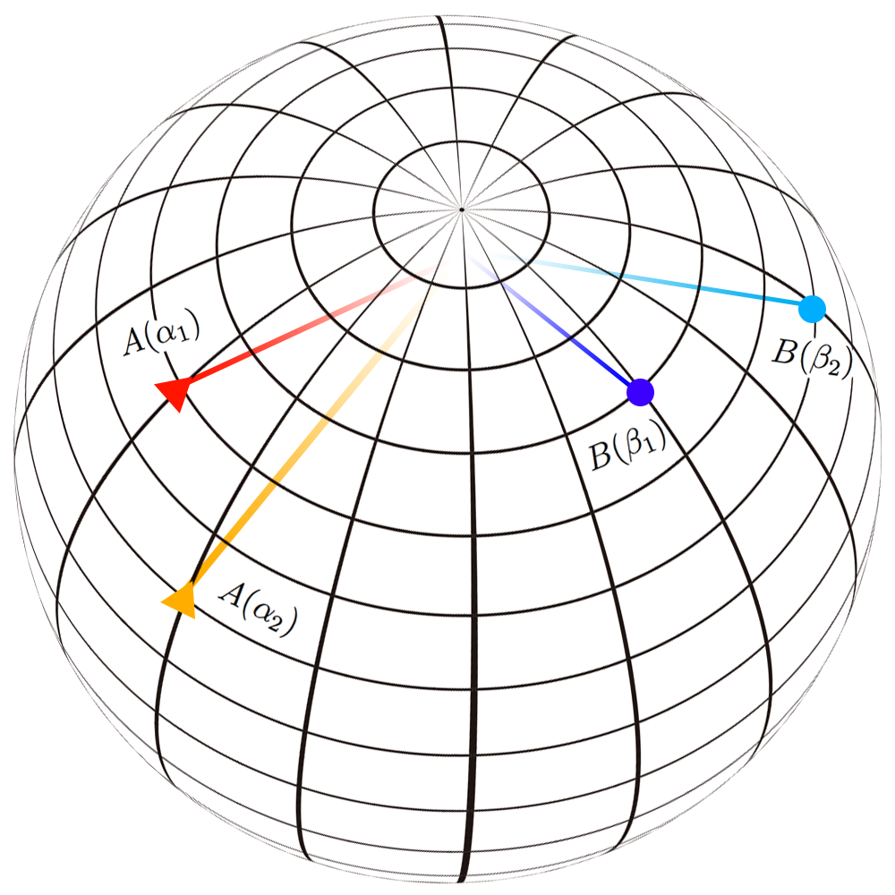
Figure 1: Observable schematic for the CGLMP prescription of non-locality. Variable phases $\alpha_{1},\alpha_{2},\beta_{1},\beta_{2}$ are fine-tuned to set the pairs of observables in subsystems A and B. They are represented as vectors with intersections on the unit sphere being depicted by triangles and circles respectively. (Colour online.)

The observables take the form $A=\sum_{R}R\left|R\right\rangle\left\langle R\right|,B=\sum_{S}S\left|S\right\rangle\left\langle S\right|$, where $R,S$ are respective eigen values. These observables are in general non-zero in their off-diagonals. Higher order tensor relationships are required to manifest such non-zero off-diagonals, as discussed earlier.

In the CGLMP prescription, the analog to the Bell-CHSH function given by Eq. 6, for the detection of non-locality is the function:

$$I_{N}=\sum_{t=0}^{[N/2]-1}\Big{(}1-\frac{2t}{N-1}\Big{)}\{[P(A_{1}=B_{1}+t)$$ (27)

$$+P(B_{1}=A_{2}+t+1)+P(A_{2}=B_{2}+t)$$

$$+P(B_{2}=A_{1}+t)]-[P(A_{1}=B_{1}-t-1)$$

$$+P(B_{1}=A_{2}-t)+P(A_{2}=B_{2}-t-1)$$

$$+P(B_{2}=A_{1}-t-1)]\}$$

where $P(A_{i},B_{i})$ are joint measurement probabilities for local observables $A_{i},B_{i}$ belonging to the two subsystems. All the observables have distinct integer eigenvalues $0,1,\cdots,N-1$.

The CGLMP operator is nothing but a linear combination of projectors, with probability $P(A_{1}=B_{1}+t)$, for instance, determined by projector
$\left|S_{1}+t\right\rangle\left\langle S_{1}+t\right|\otimes\left|S_{1}\right\rangle\left\langle S_{1}\right|$.

Each term requires a contribution from not only lower ranked, but higher ranked moments as well. It suffices to show that a single projector of the form $\left|R\right\rangle\left\langle R\right|$ has contribution from tensors of all ranks, i.e., it suffices to show a non-zero overlap of one projector. We once again consider the overlap between tensor moment $T^{k}_{q}$ and the form of the operator. Since we are dealing with spin moments, the prescription is re-defined in terms of spin: $N=2s+1$, with $j_{i}\in[-s,s]$. We look at the projection corresponding to $R$, for an observable defined by phase $\alpha_{i}$.

$$Tr\bigg{[}\left|R\right\rangle\left\langle R\right|T_{q}^{k}\bigg{]}$$ (28)

$$=\frac{1}{N}\sum_{j_{1}j_{2}}\exp{\bigg{(}\frac{2\pi i}{N}(R+\alpha_{i})(j_{1}-j_{2})\bigg{)}}\left\langle j_{1}\right|T_{q}^{k}\left|j_{2}\right\rangle$$ (29)

where matrix element:
$\left\langle j_{1}\right|T_{q}^{k}\left|j_{2}\right\rangle=C(s,k,s;j_{2},q,j_{1})\left\langle s\right||T^{k}_{q}|\left|s\right\rangle$,
and $\left\langle s\right||T^{k}_{q}|\left|s\right\rangle=\sqrt{2k+1}$.

We consider specific projection operators on 3 and 4-level systems for phases $\alpha=0,\frac{1}{2}$, those used initially in Coll02 .

Table 5: Overlaps Between Tensor Moments and a CGLMP Projector

$s$	$k=1$	$k=2$	$k=3$
1	$\sqrt{2}$	$0.2\sqrt{15}$	NA
$\frac{3}{2}$	$\approx 1.995$	$0.4\sqrt{10}$	$\approx 0.846$

Absolute values of the cumulative overlap $\sum_{q}T^{k}_{q}$ between tensor moment $T^{k}_{q}$ and projector, given by Equation 29. Note: overlaps were identical for $\alpha=0,\frac{1}{2}$ and overlaps with all $\left|R\right\rangle\left\langle R\right|$ where $R=-s\cdots s$ were identical.

The overlaps were identical for both phases, indicating that phase does not contribute to the manifestation of these tensor moments. Moreover, each projector has the same magnitude of contribution for a given tensor operator. It is clear that tensor moments of order $2s$ contribute to the detection of non-locality. By simply projecting the CGLMP functional operator onto the subspace given by $T^{1}_{q}$, one loses information related to tensor moments of higher ranks. Thus, this dependence is not unique to a particular prescription of non-locality, and true non-locality cannot be revealed without contributions from these higher ordered tensors.

VII Conclusion

In conclusion, we have shown, through qualitative and quantitative analyses, that the emergence of classicality in the so called large $N$ limit is valid only in a weak sense, being entirely due to the limited experimental resources available to determine tensor moments of observables and correlations. The result has been demonstrated for both entanglement and non-locality, with two different prescriptions for the latter. In short, the so-called classical limit is not an inherent property of the system. Consequently, the emergent classicality in higher dimensions is ‘weak’ in the sense defined and described in this paper.

References

- [1] L. G Yaffe. Large limits as classical mechanics. Reviews of Modern Physics, 54:407, April 1982.
- [2] G. C. Ghirardi, A. Rimini, and T. Weber. Unified dynamics for microscopic and macroscopic systems. Phys. Rev. D, 34:470, Jul 1986.
- [3] N. D. Mermin. Quantum mechanics vs local realism near the classical limit: A bell inequality for spin s. Phys. Rev. D, 22:356, 1980.
- [4] A. Peres. Finite violation of a bell inequality for arbitrarily large spin. Phys. Rev. A, 46:4413, Oct 1992.
- [5] M. Ardehali. Hidden variables and quantum-mechanical probabilities for generalized spin- systems. Phys. Rev. D, 44:3336, Nov 1991.
- [6] M. Ardehali. Bell inequalities with a magnitude of violation that grows exponentially with the number of particles. Phys. Rev. A, 46:5375, Nov 1992.
- [7] D. Kaszlikowski, P. Gnaciński, M. Żukowski, W. Miklaszewski, and A. Zeilinger. Violations of local realism by two entangled -dimensional systems are stronger than for two qubits. Phys. Rev. Lett., 85:4418, Nov 2000.
- [8] D. Collins, N. Gisin, N. Linden, S. Massar, and S. Popescu. Bell inequalities for arbitrarily high-dimensional systems. Phys. Rev. Lett., 88:040404, Jan 2002.
- [9] L.B. Fu. General correlation functions of the clauser-horne-shimony-holt inequality for arbitrarily high-dimensional systems. Phys. Rev. Lett., 92:130404, Mar 2004.
- [10] S. Braunstein, A. Mann, and M. Revzen. Maximal violation of bell inequalities for mixed states. Phys. Rev. Lett., 68:3259, Jun 1992.
- [11] S. Popescu and D. Rohrlich. Which states violate bell’s inequality maximally? Physics Letters A, 169(6):411, 1992.
- [12] J. S. Bell. On the einstein podolsky rosen paradox. Physics, 1:195, 1964.
- [13] J. F. Clauser, M. A. Horne, A. Shimony, and R. A. Holt. Proposed experiment to test local hidden-variable theories. Phys. Rev. Lett., 23(15):880, October 1969.
- [14] N. Brunner, D. Cavalcanti, S. Pironio, V. Scarani, and S. Wehner. Bell nonlocality. Rev. Mod. Phys., 86:419–478, Apr 2014.
- [15] Michael A. Nielsen and Isaac L. Chuang. Quantum Computation and Quantum Information: 10th Anniversary Edition. Cambridge University Press, New York, NY, USA, 10th edition, 2011.
- [16] V. Ravishankar and G. Ramachandran. Redundant polarisation measurements in particle interactions with arbitrary spin j. Modern Physics Letters A, 01(05):333, 1986.
- [17] V. Ravishankar and G. Ramachandran. 2jth rank tensor polarization in reactions involving a spin j particle. Phys. Rev. C, 35:62, Jan 1987.
- [18] W. H. Zurek. Proc. of the XXII GIFT International Seminar on Theoretical Physics. World Scientific, Singapore, 1991.
- [19] M. Brune, E. Hagley, J. Dreyer, X. Maître, A. Maali, C. Wunderlich, J. M. Raimond, and S. Haroche. Observing the progressive decoherence of the “meter” in a quantum measurement. Phys. Rev. Lett., 77:4887, Dec 1996.
- [20] W. H. Zurek. The Environment, Decoherence and the Transition from Quantum to Classical-revisited (2003). arXiv preprint quant-ph/0306072, 2003.
- [21] J. Kofler and Č. Brukner. Classical world arising out of quantum physics under the restriction of coarse-grained measurements. Phys. Rev. Lett., 99:180403, Nov 2007.
- [22] I. P. Mendaš. Geometric conditions for violation of bell’s inequality. Phys. Rev. A, 71:034103, Mar 2005.
- [23] R. P. Sandhir, S. Adhikary, and V. Ravishankar. Cglmp and bell–chsh formulations of non-locality: a comparative study. Quantum Information Processing, 16(10):263, Sep 2017.
- [24] N. Gisin and A. Peres. Maximal violation of Bell inequality for arbitrarily large spin. Phys. Lett. A, 162(1):15, 1992.
- [25] K. Wódkiewicz. Randomness, non locality, and information in entangled correlations. Phys. Rev. A, 52:3503, 1995.
- [26] K. Banaszek and K. Wodkiewicz. Nonlocality of the einstein-podolsky-rosen state in the wigner representation. Phys. Rev. A, 58:4345, Dec 1998.
- [27] T. Durt, D. Kaszlikowski, and M. Żukowski. Violations of local realism with quantum systems described by N -dimensional hilbert spaces up to . Phys. Rev. A, 64:024101, Jul 2001.