Covariant approach of perturbations in Lovelock type brane gravity

Abstract

We develop a covariant scheme to describe the dynamics of small perturbations on Lovelock type extended objects propagating in a flat Minkowski spacetime. The higher-dimensional analogue of the Jacobi equation in this theory becomes a wave type equation for a scalar field $\Phi$. Whithin this framework, we analyse the stability of membranes with a de Sitter geometry where we find that the Jacobi equation specializes to a Klein-Gordon (KG) equation for $\Phi$ possessing a tachyonic mass. This shows that, to some extent, these types of extended objects share the symmetries of the Dirac-Nambu-Goto (DNG) action which is by no means coincidental because the DNG model is the simplest included in this type of gravity.

,  ,   ,

1 Introduction

Extended objects, sometimes referred to as membranes or branes for short, are surfaces of arbitrary dimension that are intended to represent many physical systems at diverse energy scales [1]. The most interesting action to describe a relativistic extended object propagating in a fixed background spacetime, based in the worldvolume geometry, is given by a local action involving a linear combination of higher-order curvature terms constructed by considering geometrical scalars [2, 3]. However, by appealing for both worldvolume reparametrization and background spacetime diffeomorphism invariances these geometrical scalars are limited. Among the plethora of worked geometric models, in first place we have the DNG model which is proportional to the volume swept out by the brane, the quadratic term in the mean extrinsic curvature introduced by Polyakov for a possible stringy description of QCD [4], the Helfrich-Canham model in biophysics for describing fluid membranes [5], models for describing particle spinning particles either massive or masless [6, 7, 8]. Unfortunately, a clumsy fact is that the associated equations of motion (eom) are in general fourth-order equations in the field variables. Not all the worldvolume geometrical scalars fall into this category. For a given dimension $p$ there is a special subset of second-order terms which stabilize the extended object dynamics by maintaining the second-order eom thereby having potential physical applications. These are similar in form either to the original form of the Lovelock invariants in gravity or to their counterterms necessary in order to have a well-posed variational problem [9, 10, 11, 12, 13]. This aspect makes a given theory, free from many of the pathologies that plague higher-order derivative theories (see also [14] for a review on this topic). This fact is important because it assures no propagation of extra degrees of freedom. An appropriate description for extended objects realized in the form of a Born-Infeld type structure was developed in [15] and named Lovelock type brane gravity. The interest in this subject has attracted quite a lot of attention recently by the attractive geometric structure and possible applications in accelerated cosmological scenarios [16, 17, 18, 19]. In [15], the query on the existence and stability of the physical systems modeled by extended objects of this type was formulated so that here we enter the answer to the posed question.

The purpose of this paper is to provide a covariant framework to study the stability of small perturbations on Lovelock type extended objects moving in a flat Minkowski spacetime. The brane perturbations are guided by a Jacobi equation which is manifested through a wave type equation where the perturbations are described by a scalar field, $\Phi$, living in the $(p+1)$-dimensional worldvolume. This equation is characterized by a mass-like term expressed in terms of the worldvolume geometry. Because the mechanic content of an extended object, described by an action constructed from geometric scalars, is captured through their geometric degrees of freedom (dof), it is expected that $\Phi$ will be in correspondence with the only dof that this type of models possesses.

By specializing this framework to de Sitter branes with a spherical symmetry we are able to simplify the Jacobi equation to a KG one with a negative mass. This equation was extensively discussed by Garriga and Vilenkin in the case of DNG branes [20, 21, 22]. We find that modes with angular momentum $L$ leading even eigenvalues $J$ associated to the spherical harmonics, produce an oscillatory behaviour that gets frozen at some time but subsequently restarts with some growing modes of oscillation which rapidly leading to instability thus ending up with highly nonspherical bubbles. For odd $J$ values the oscillatory behavior is drastically affected leading thus to instability more quickly. This result has been inherited for this extension to Lovelock type extended objects from the DNG model because, in some sense, the so-called Lovelock type brane gravity can be seen as a higher analogue of the DNG model with a extrinsic volume element [15]. Therefore, it is all set to explore the physical implications arising from this perturbation analysis for this sort of gravity.

The paper is organized as follows. In Sec. 2 we provide an overview of the Lovelock type brane gravity theory where we highlight the role that play some conserved tensors useful to study the mechanical content for this theory. We derive the first variation of the action governing the Lovelock type brane theory in Sec. 3 in order to obtain the eom and to pave the way to carry out the analysis of perturbations. In Sec. 4 we examine the second variation of the action and obtain the corresponding Jacobi equation which exhibits how the perturbations evolve. To illustrate our development, we specialize our framework to de Sitter membranes in Sec. 5. We conclude in Sec. 6 with some comments and discuss our results. Appendix gathers useful information about the geometry of de Sitter branes floating in a Minkowski spacetime. For the sake of simplicity, we restrict our attention to closed extended objects with no physical boundaries.

2 Lovelock type brane theory

Consider a dynamical extended object, $\Sigma$, of dimension $p$ moving in a $N=(p+2)$-dimensional Minkowski spacetime ${\cal M}$ with metric $\eta_{\mu\nu}$ $(\mu,\nu=0,1,\ldots,p+1)$. The worldvolume $m$, is an oriented timelike hypersurface manifold of dimension $p+1$, described by the embedding functions $y^{\mu}=X^{\mu}(x^{a})$ where $y^{\mu}$ are local coordinates of ${\cal M}$ and $x^{a}$ are local coordinates of $m$, and $X^{\mu}$ are the embedding functions $(a,b=0,1,\ldots,p)$. The most important derivatives of $X^{\mu}$ enter the game through the induced metric tensor $g_{ab}=\eta_{\mu\nu}e^{\mu}{}_{a}e^{\nu}{}_{b}:=e_{a}\cdot e_{b}$ and the extrinsic curvature $K_{ab}=-n\cdot\nabla_{a}e_{b}=K_{ba}$ where $e^{\mu}{}_{a}=\partial_{a}X^{\mu}$ are the tangent vectors to $m$, $n^{\mu}$ is the spacelike unit normal vector to $m$, and $\nabla_{a}$ is the covariant derivative compatible with $g_{ab}$.

For a $(p+1)$-dimensional worldvolume described by the variables $X^{\mu}$ the action [15]

$$S[X]=\int_{m}d^{p+1}x\,\sqrt{-g}\sum_{n=0}^{p+1}\alpha_{n}\,L_{n}(g_{ab},K_{ab}),$$ (1)

where

$$L_{n}(g_{ab},K_{ab})=\delta^{a_{1}a_{2}a_{3}\cdots a_{n}}_{b_{1}b_{2}b_{3}\cdots b_{n}}K^{b_{1}}{}_{a_{1}}K^{b_{2}}{}_{a_{2}}K^{b_{3}}{}_{a_{3}}\cdots K^{b_{n}}{}_{a_{n}},$$ (2)

ensures that the field equations of motion are of second order. Here, $\delta^{a_{1}a_{2}a_{3}\ldots a_{n}}_{b_{1}b_{2}b_{3}\ldots b_{n}}$ denotes the generalized Kronecker delta (gKd), $g=\textrm{det}(g_{ab})$ and $\alpha_{n}$ are constants with appropriate dimensions. We set $L_{0}=1$. This action is invariant under reparametrizations of the worldvolume. The Lagrangian (2) is a polynomial of degree $n\leq p+1$ in the extrinsic curvature so that the action (1) is a second-order derivative theory. The geometrical invariants (2) are to be referred to as Lovelock type brane invariants (LBI). By construction, these scalars vanish for $n>p+1$ whereas the term with $n=p+1$ corresponds to a topological invariant not contributing to the field equations. Since $X^{\mu}$ are the independent variables instead of the metric, we then have one greater number of Lovelock type terms contrary to the pure gravity case. We can find a complete list of the first LBI in [15].

For even $n$ we recognize the form of the Gauss-Bonnet (GB) terms but expressed now in terms of the worldvolume geometry. For example, for $n=0$ we have the DNG Lagrangian, for $n=2$ we have the Regge-Teitelboim (RT) model [23, 24, 25, 26, 27, 28, 29], for $n=4$ we have the form of the GB Lagrangian which for $p>3$ produces non-vanishing eom with ghost-free contribution. On the other side, for odd $n$ the corresponding Lagrangians look like the Gibbons-Hawking-York boundary terms which may exist if we have the presence of bulk Lovelock invariants (see [9, 15] for details).

Some remarks are in order. To avoid ambiguities for possible gauge invariance for the case of odd $n$ Lagrangians, we assume that $n^{\mu}$ is such that it is pointing outward to $m$. Furthermore, one should not get confused and think that these LBI come from the original pure Lovelock theory as counter-terms; as discussed in [1, 30], such geometrical scalars (2) generate dynamics without the need to be considered as surface terms, where the only relevant degrees of freedom are the ones associated with the geometric configuration of the worldvolume itself. Moreover, observe that definition (2) coincides with the expression of the determinant of $K^{a}{}_{b}$. Indeed, the functional

$$S=\int_{m}d^{p+1}x\,\sqrt{-g}\,\mbox{det}\,(K^{a}{}_{b}),$$ (3)

correspond to the Gauss-Bonnet topological invariant which is a conformal invariant functional with respect to conformal transformations of the worldvolume geometry [31]. Hereafter, as a simplification in the notation, the differential $d^{p+1}x$ wherever a worldvolume integration is performed will be absorbed.

By virtue of the properties of the gKd function one can define the important tensors

$$J^{a}_{(n)b}:=\delta^{aa_{1}a_{2}a_{3}\ldots a_{n}}_{bb_{1}b_{2}b_{3}\ldots b_{n}}K^{b_{1}}{}_{a_{1}}K^{b_{2}}{}_{a_{2}}K^{b_{3}}{}_{a_{3}}\ldots K^{b_{n}}{}_{a_{n}}.$$ (4)

These are symmetric and conserved because $\nabla_{a}J^{ab}_{(n)}=0$. This fact is shown by using the properties of the gKd and the Codazzi-Mainardi integrability condition for surfaces of arbitrary dimension when the ambient spacetime is Minkowski, $\nabla_{a}K_{bc}=\nabla_{b}K_{ac}$. Notice that, for a $(p+1)$-dimensional worldvolume there are at most an equal number of conserved tensors $J^{ab}_{(n)}$. As showed in [15], by expanding out the determinant involved in (4) in terms of minors we obtain a useful recursion relation

$$J^{a}_{(n)b}=\delta^{a}_{b}\,L_{n}-nK^{a}{}_{c}J^{c}_{(n-1)b}.$$ (5)

As before, in [15] we have a detailed list of the first conserved Lovelock tensors. The $J^{ab}_{(n)}$ are to be referred to as Lovelock brane tensors (LBT). We already have some familiarity with the conservation property of (4). Indeed, $J_{(0)}^{ab}=g^{ab}$ is conserved because we have a Levi-Civita connection; $J_{(1)}^{ab}=g^{ab}K-K^{ab}$ is conserved due to the contraction of the Codazzi-Mainardi integrability condition whereas $J_{(2)}^{ab}={\cal R}g^{ab}-2{\cal R}^{ab}$ is nothing but the worldvolume Einstein tensor which is conserved by the Bianchi identity.

The contraction of Eq. (4) with the extrinsic curvature tensor, by considering Eq. (2), provides an identity among the LBT and the LBI

$$J^{ab}_{(n)}K_{ab}=L_{n+1}.$$ (6)

3 Extremality

The main fact behind the Lovelock brane invariants is that their associated eom are of second-order in the derivatives of the dynamical variables $X^{\mu}$. To prove this we consider directly the variation of the action (1)

$$\delta S=\int_{m}\left[\delta\left(\sqrt{-g}\right)\sum_{n=0}^{p+1}\alpha_{n}L_{n}+\sqrt{-g}\sum_{n=0}^{p+1}\alpha_{n}\delta L_{n}\right].$$ (7)

Carrying out the variations under the integral sign we have first that $\delta\sqrt{-g}=(\sqrt{-g}/2)g^{ab}\delta g_{ab}$. With regards the second one we have from (2) that

$$\delta L_{n} = n\delta^{a_{1}a_{2}a_{3}\cdots a_{n}}_{b_{1}b_{2}b_{3}\cdots b_{n}}K^{b_{2}}{}_{a_{2}}K^{b_{3}}{}_{a_{3}}\cdots K^{b_{n}}{}_{a_{n}}\delta K^{b_{1}}{}_{a_{1}},$$ (8)

$$= nJ^{a}_{(n-1)b}\delta K^{b}{}_{a},$$

where we have used the antisymmetric properties of the gKd and the definition (4). We also require that $\delta K^{a}{}_{b}=\delta(g^{ac}K_{cb})=-g^{ad}K^{c}{}_{b}\delta g_{dc}+g^{ac}\delta K_{cb}$. Thus, the variation (8) becomes

$$\delta L_{n} = \left(J^{ab}_{(n)}-g^{ab}L_{n}\right)\delta g_{ab}+nJ^{ab}_{(n-1)}\delta K_{ab},$$ (9)

where we have used the identity (5). Relation (9) allows us to write the variation (7) in the form

$$\delta S=\int_{m}\sqrt{-g}\sum_{n=0}^{p+1}\alpha_{n}\left[\left(J^{ab}_{(n)}-\frac{1}{2}g^{ab}L_{n}\right)\delta g_{ab}+nJ^{ab}_{(n-1)}\delta K_{ab}\right].$$ (10)

At this stage what we have is the response of the action (1) to small changes in the worldvolume

$$X^{\mu}(x^{a})\rightarrow X^{\mu}(x^{a})+\delta X^{\mu}(x^{a}),$$ (11)

through the variations $\delta g_{ab}$ and $\delta K_{ab}$. Now, it should be emphasized that only motions tranverse to the worldvolume are physically observable so that we shall consider only $\delta_{\perp}X^{\mu}=\Phi\,n^{\mu}$ where $\Phi$ is assumed to be small but is otherwise an arbitrary function of $x^{a}$. This is reflected in the fact that the most important variations to be considered are [30]

$$\delta_{\perp}g_{ab} = 2K_{ab}\,\Phi,$$ (12)

$$\delta_{\perp}K_{ab} = -\nabla_{a}\nabla_{b}\Phi+K_{ac}K^{c}{}_{b}\,\Phi.$$ (13)

If we replace these expressions into (10) we get

$$\delta S = \int_{m}\sqrt{-g}\sum_{n=0}^{p+1}\alpha_{n}\left(2J^{ab}_{(n)}K_{ab}-KL_{n}+nK^{c}{}_{a}J^{ab}_{(n-1)}K_{cb}\right)\Phi$$

$$+ \int_{m}\nabla_{a}\left(-\sqrt{-g}\sum_{n=0}^{p+1}\alpha_{n}\,nJ^{ab}_{(n-1)}\nabla_{b}\Phi\right),$$

where we have used the conservation of the LBT. By using the identities (5) and (6) we finally obtain the variation of the action $S$ in the form

$$\delta S=\int_{m}\sqrt{-g}\,{\cal E}\Phi+\int_{m}\sqrt{-g}\,\nabla_{a}Q^{a}[\Phi],$$ (14)

where

$${\cal E}=\sum_{n=0}^{p+1}\alpha_{n}J^{ab}_{(n)}K_{ab}=0,$$ (15)

is the Euler-Lagrange (EL) equation of motion which in turn can be expressed in terms of the LBI through the identity (6). In addition,

$$Q^{a}:=\sum_{n=0}^{p+1}\alpha_{n}Q^{a}_{(n)}=-\sum_{n=1}^{p+1}\alpha_{n}\,nJ^{ab}_{(n-1)}\nabla_{b},$$ (16)

is a differential operator defined on the worldvolume. Obviously, we have only one equation of motion which is second-order in the field variables. This fact, in particular, means that we have only one physical degree of freedom for this type of branes. Indeed, the physically observable measure of the deformation of the surface is the breathing mode provided by the scalar field $\Phi$. In summary, under the deformation (11), the first variation of the action (1) yields

$$\delta S=\int_{m}\sqrt{-g}\sum_{n=0}^{p+1}\alpha_{n}\,J^{ab}_{(n)}K_{ab}\,\Phi=0,$$ (17)

where (15) is the result of the physical transverse motions. As expected, we may think of the eom (15) as the generalization of the condition for extremal hypersurfaces in the sense that we have the vanishing of the trace of the extrinsic curvature where the conserved tensors $J^{ab}_{(n)}$ play the role of a metric.

4 Linearized normal perturbations on the worldvolume

We turn now to compute the second variation of the action $S$. Unlike the first variation to obtain the equation of motion, in general in order to have a well posed second variation it is not allowed to neglect the tangential deformations of the surface. This is related to the fact that a finite tangential deformation, unlike its infinitesimal counterpart, is not a simple reparametrization of the surface [32]. From the second variation

$$\delta^{2}S=\int_{m}\sum_{n=0}^{p+1}\alpha_{n}\delta\left(\sqrt{-g}\,J^{ab}_{(n)}K_{ab}\,\Phi\right),$$ (18)

clearly we have that the relevant equation is

$$\sum_{n=0}^{p+1}\alpha_{n}\delta\left(J^{ab}_{(n)}K_{ab}\right)=0.$$ (19)

It has been formally proved in [32] that if ${\cal E}$ represents the EL equation of motion, then the total variation $\delta\left(\sqrt{-g}\,{\cal E}\,\Phi\right)=\delta_{\perp}\left(\sqrt{-g}\,{\cal E}\right)\Phi={\cal L}\Phi$ where ${\cal L}$ is a local differential operator so that it is only necessary to consider the variations (12) and (13). Accordingly, to evaluate (19) we begin first by using the definition (4) to obtain

$$\delta_{\perp}J^{ab}_{(n)}=\delta_{\perp}g^{bc}\,J^{a}_{(n)c}+ng^{bc}\,\delta^{aa_{1}a_{2}\cdots a_{n}}_{cb_{1}b_{2}\cdots b_{n}}K^{b_{2}}{}_{a_{2}}\cdots K^{b_{n}}{}_{a_{n}}\,\delta_{\perp}K^{b_{1}}{}_{a_{1}}.$$

Now, as a result of the contraction of this relation with the extrinsic curvature we have

$$\hskip 56.9055ptK_{ab}\delta_{\perp}J^{ab}_{(n)}=\delta_{\perp}g^{bc}J^{a}_{(n)c}K_{ab}+n\,\delta^{a_{1}aa_{2}\cdots a_{n}}_{b_{1}cb_{2}\cdots b_{n}}K^{c}{}_{a}K^{b_{2}}{}_{a_{2}}\cdots K^{b_{n}}{}_{a_{n}}\delta_{\perp}K^{b_{1}}{}_{a_{1}},$$

$$\hskip 32.72049pt=\delta_{\perp}g^{bc}J^{a}_{(n)c}K_{ab}+nJ^{a}_{(n)b}\delta_{\perp}K^{b}{}_{a},$$

where in the first line of the right-hand side we have used, once again, the antisymmetric properties of the gKd. Further, observe that $\delta_{\perp}K^{b}{}_{a}=\delta_{\perp}g^{bc}K_{ca}+g^{bc}\delta_{\perp}K_{ca}$ and therefore

$$K_{ab}\delta_{\perp}J^{ab}_{(n)}=(n+1)J^{a}_{(n)c}K_{ab}\delta_{\perp}g^{bc}+nJ^{ab}_{(n)}\delta_{\perp}K_{ab}.$$

In this manner, from (19) we find that

$$\delta_{\perp}\left(J^{ab}_{(n)}K_{ab}\right)=(n+1)J^{a}_{(n)c}K_{ab}\delta_{\perp}g^{bc}+(n+1)J^{ab}_{(n)}\delta_{\perp}K_{ab}.$$ (20)

As mentioned before, only motions transverse to the worldvolume are physically observable so, from (12) one has $\delta_{\perp}g^{ab}=-g^{ac}g^{bd}\delta_{\perp}g_{cd}=-2K^{ab}\Phi$. Hence, by plugging this variation and (13) into expression (20) we get

$$\delta\left(J^{ab}_{(n)}K_{ab}\right) = -(n+1)\left[J^{ab}_{(n)}\nabla_{a}\nabla_{b}\Phi+J^{ab}_{(n)}K_{a}{}^{c}K_{bc}\,\Phi\right].$$

It therefore follows that when we treat the second variation (18) as an action, $S^{\prime}:=\delta^{2}S$, we find

$$S^{\prime}=-\int_{m}\sqrt{-g}\sum_{n=0}^{p+1}\alpha_{n}\,(n+1)\Phi\left[J^{ab}_{(n)}\nabla_{a}\nabla_{b}\Phi+J^{ab}_{(n)}K_{a}{}^{c}K_{bc}\,\Phi\right].$$ (21)

The variation of this action with respect to $\Phi$ leads immediately to the expression $\sum_{n=0}^{p+1}\alpha_{n}(J^{ab}_{(n)}\nabla_{a}\nabla_{b}\Phi+J^{ab}_{(n)}K_{a}{}^{c}K_{bc}\,\Phi)=0$, or more suggestively as

$$\sum_{n=0}^{p+1}\alpha_{n}(n+1)\left[J^{ab}_{(n)}\nabla_{a}\nabla_{b}\Phi+M_{(n)}^{2}\,\Phi\right]=0,$$ (22)

where

$$M^{2}_{(n)}:=J^{ab}_{(n)}K_{a}{}^{c}K_{bc},$$ (23)

is a purely geometric quantity that plays the role of a mass-like term. The equation (22) corresponds to the Jacobi equation in the Lovelock type brane gravity. On geometrical grounds, the Jacobi equation describes the behavior of Lovelock type surfaces which are close or in the neighborhood of a reference surface one. Clearly, we may think of this equation as the second-order generalization of the corresponding Jacobi equation for the case of DNG branes so that we provide a generalization of the wave equation developed for an arbitrary DNG extended object moving in a Minkowski spacetime [20, 21, 22, 30, 33, 34, 35]. Consequently, we will regard (22) as the equation of motion for the small perturbations $\Phi$. Thus, the second variation of (1) can be expressed as

$$\delta^{2}S[X^{\mu}]=\int_{m}\sqrt{-g}\,\Phi\,{\cal L}\Phi,$$ (24)

where

$${\cal L}=\sum_{n=0}^{p+1}\alpha_{n}{\cal L}_{(n)}=\sum_{n=0}^{p+1}\alpha_{n}(n+1)\left[J^{ab}_{(n)}\nabla_{a}\nabla_{b}+M^{2}_{(n)}\right].$$ (25)

Moreover, taking advantage of the conservation property of the LBT, a convenient way to express Eq. (22) is as follows

$$\sum_{n=0}^{p+1}\alpha_{n}(n+1)\left[\frac{1}{\sqrt{-g}}\partial_{a}\left(\sqrt{-g}J^{ab}_{(n)}\partial_{b}\Phi\right)+M^{2}_{(n)}\,\Phi\right]=0.$$ (26)

The solutions of the Jacobi equations (22) address the question of stability through the nature of the modes $\Phi$. If we find that the resulting modes are oscillatory, then they indicate stability of the system whereas growing modes confirm the existence of an instability. In this sense, the only degree of freedom describing the deformation of any Lovelock type extended object is the breathing mode of the worldvolume. It should be mentioned that we may arrive at the same Eq. (22) in a somewhat different manner. That is, from a non-perturbative framework by considering a purely kinematical description of the normal deformations of the worldvolume [35]. There, the Jacobi equation corresponds to a higher-dimensional analogue of the Raychaudhuri equation describing point particles.

From the Lovelock brane tensors (4) and (23) we have at few order that

$$M_{(0)}^{2} = K_{ab}K^{ab},$$ (27)

$$M_{(1)}^{2} = K^{ab}{\cal R}_{ab},$$ (28)

$$M_{(2)}^{2} = {\cal R}K_{ab}K^{ab}-2{\cal R}^{b}{}_{c}K^{c}{}_{a}K^{a}{}_{b},$$ (29)

so that the wave-like equation can be rewritten explicitly. For example, for $n=0$, we know that $J^{ab}_{(0)}=g^{ab}$. Thereby, Eq. (26) becomes

$$\Box\Phi+K_{ab}K^{ab}\Phi=0,$$

where $\Box=g^{ab}\nabla_{a}\nabla_{b}$ stands for the d’Alembertian operator defined on $m$. This case has been studied exhaustively in many contributions [20, 21, 22, 33, 36].

5 Perturbations on de Sitter membranes

We now confine our attention to a specific geometry. Suppose that $\Sigma$ is a $p$-dimensional de Sitter membrane moving in a Minkowski spacetime described by the action (1). The metric on $m$ can be expressed in the form

$$dS_{p+1}^{2}=-d\tau^{2}+H^{-2}\cosh^{2}(H\tau)d\Omega_{(p)}^{2},$$ (30)

where $d\Omega_{(p)}^{2}=d\theta_{1}^{2}+\sin^{2}\theta_{1}d\theta_{2}^{2}+\sin^{2}\theta_{1}\sin^{2}\theta_{2}d\theta_{3}^{2}+\ldots+\sin^{2}\theta_{1}\sin^{2}\theta_{2}\cdots\sin^{2}\theta_{p-1}d\theta_{p}$ is the metric on the $p$-sphere and $H$ is a constant (see A for details). Thus, $\sqrt{-g}=H^{-p}\cosh^{p}(H\tau)\prod_{r=1}^{p}\sin^{p-r}\theta_{r}$. Being a maximally symmetric spacetime, the Lovelock type tensors as well as the Lovelock type invariants become

$$J^{ab}_{(n)} = C_{(p,n)}H^{n}g^{ab},$$ (31)

$$L_{n} = C_{(p+1,n)}H^{n},$$ (32)

where we have introduced the notation $C_{(p,n)}=\Gamma(p+1)/\Gamma(p-n+1)$ and $\Gamma(n)$ is the Gamma function. The expression (31), together with the relation (44), when substituted into the expression for the mass-like term (23) lead to

$$M_{(n)}^{2}=(p+1)C_{(p,n)}H^{n+2}.$$ (33)

It is evident now that the quantities (31) and (33), when inserted into the relation (26), give rise

$$\sum_{n=0}^{p+1}\alpha_{n}(n+1)H^{n}C_{(p,n)}\left[\Box\Phi+(p+1)H^{2}\Phi\right]=0,$$ (34)

which in turn implies that

$$\Box\Phi+(p+1)H^{2}\Phi=0.$$ (35)

Therefore, the theory of perturbations on de Sitter Lovelock type membranes simplifies enormously to the analysis of a Klein-Gordon equation for a scalar field $\Phi$ with a negative mass $m^{2}:=-(p+1)H^{2}$, as in the case of DNG extended objects [20, 33, 34]. To understand this point we only insert the emergent expression for the Lagrangians (32) into the action (1) and observe that a DNG action emerges.

To solve Eq. (35) it is convenient to consider a decomposition into spherical modes

$$\Phi(\tau,\theta_{i})=\sum_{LM}\phi_{L}(\tau)Y_{LM}(\theta_{i}).\qquad\quad\begin{array}[]{ll}L&=0,1,\ldots,\infty.\\ M&=-L,-L+1,\ldots,0,\ldots,L-1,L.\\ i&=1,2,\ldots,p.\end{array}$$ (36)

Here, $Y_{LM}$ stands for the spherical harmonics on the $p$-sphere satisfying $\Delta Y_{LM}=-J\,Y_{LM}$ where $\Delta$ is the Laplacian operator defined on the unit $p$-sphere and $J$ denotes the eigenvalues of the spherical harmonics given by $J=L(L+p-1)$. The solution $\phi_{L}(\tau)$ is given by a linear combination of the associated Legendre functions $P^{\mu}_{\nu}(\tanh(H\tau))$ and $Q^{\mu}_{\nu}(\tanh(H\tau))$ (see [20]) for details).

For $p=3$ it was shown that lowest modes, $L=0$ and $L=1$, do not correspond to true perturbations but that they must be understood physically as a time translation and a spatial rotation of the unperturbed solution, respectively [20]. These solutions are plotted in figure (1). However, at cosmological level these lowest modes become significant in a inflationary scenario but not so with the other ones since they exhibit a damped oscillatory behaviour for short times [37]. We expect that for larger times the modes characterized by the oscillatory behaviour become important for the self-accelerated expansion of a late time brane-like universe [29], as seen in the figure (2).

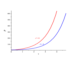
Figure 1: The bubble behaviour for $J=0$ and $J=3$ values. These are not perturbations but time translation and spatial rotation of the bubble for the lowest modes $L=0$ and $L=1$, respectively.

Indeed, by considering even $J$ values, and for short times, we have perturbations provided with an oscillatory behaviour. As time increases, behaviour gets frozen at some finite value of the radius but subsequently restarts with some growing modes of oscillation which rapidly leading to instability thus ending up with highly nonspherical bubbles. To explore the region of stability we can provide the representation of the solution for the perturbation from the point of view of the dynamical systems evolving in the phase space. For short times we observe that the trajectories for even values of $J$ tend to the point located at the origin which is a signal of stability. But such stability is deceptive. For the limit of larger time, it is observed that the trajectories are reset and these fastly move away from the origin what is a sign of an instability of the membrane [20].

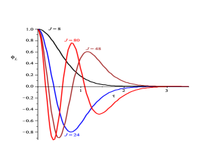
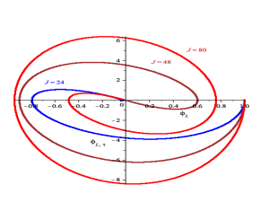
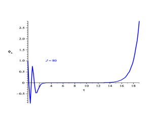
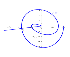
Figure 2: Oscillatory behaviour obtained for the even values of the parameter $J$ considering short and large times. The left pictures are depicted in the configuration space while on the right were plotted in the corresponding phase space.

In contrast, for odd values of $J$ it is noted from the beginning an oscillatory behaviour of the perturbation but as time passes the amplitude grows rapidly so that instabilities of the membrane can take place more quickly. Figure (3) shows this last possibility of the behaviour for the solution $\phi_{L}$. With regards higher-dimensional de Sitter membranes we must mention that the behaviour is quite similar.

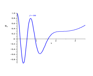
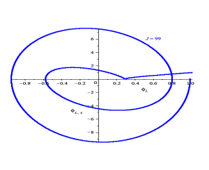
Figure 3: Oscillatory behaviour exhibited from the value of the parameter $J=99$. The left picture is showed in the configuration space while the right picture was obtained on the corresponding phase space.

6 Concluding remarks

In this paper we reviewed the so-called Lovelock type brane gravity which, for even values of $p$ mimics the original Lovelock gravity terms while for odd values of $p$ resembles the necessary counterterms in order to have a well posed variational principle in gravity. Then, based on modern variational techniques, we have obtained the criteria for which a Lovelock type extended object becomes extremal. We derived the general equations of motion written in a compact form by taking into account useful conserved brane tensors. Afterwards, we construct a covariant framework to study the conditions for which an extended object of this type becomes stable against infinitesimal perturbations. Thence, we obtain the corresponding Jacobi equation which is manifested through a wave type equation governing the dynamics of the perturbations. To appreciate our framework, the special case of de Sitter membranes with spherical symmetry has been studied. In particular, the wave type equation is reduced to the usual Klein-Gordon equation, as in the standard DNG case so that we can take advantage of the analysis carried out in such a case. Hence, we observe that for this geometry the analysis is insensitive to any model of the so-called Lovelock type brane gravity. This is by no means coincidental because the DNG model is part of this type Lovelock gravity as the first element of the expansion (1) so it is expected that some of the properties already known for the DNG model reappear in the full theory. On the other hand, it should be mentioned also that the resulting Jacobi equation (22) can be obtained from another viewpoint by considering a purely kinematical description of the normal deformations of the worldvolume [35]. In such an approach, this equation corresponds to the so-called generalized Raychaudhuri equation which is an analogous to higher-dimensions of the Raychaudhuri equation describing point particles. In this regard, we must mention that another interesting framework to analyse the stability of brane universes was developed recently [38]. An even important question that we will investigate is whether we can extend our framework to the case of consider extended objects (or branes) as sources of gravity in the $N=(p+2)$-dimensional background spacetime. In such a case, we need to take careful in incorporating properly the Israel’s junction conditions [39, 40, 41]. In addition, it remains to explore the possible cosmological implications arising from this type of approach in the subject of brane cosmology. In particular, we can undertake a perturbation analysis of the so-called geodetic brane gravity which consists either of the first two or three terms of the Lovelock type brane gravity which has been reignited recently [25, 26, 28, 29, 42, 43, 44]. Another interesting issue to be explored is the existence of a critical dimension for this type of gravity [47, 48, 49, 50] as occur in the pure Lovelock gravity which could provide information on the solutions of the field equations. Investigation in these directions is presently underway. Finally, we hope that the perturbation analysis we have done here can provide a useful starting point to explore the issue of brane nucleation [42, 45, 46].

Appendix A A de Sitter membrane immersed in a Minkowski bulk

Consider the immersion of a $(p+1)$-dimensional de Sitter membrane embedded in a $N=(p+2)$-dim flat Minkowski spacetime in terms of the so-called Rindler coordinates [19]

$$x^{\mu}=X^{\mu}(\tau,\theta_{i})=\left(\begin{array}[]{l}H^{-1}\sinh(H\tau)\\ H^{-1}\cosh(H\tau)\cos\theta_{1}\\ H^{-1}\cosh(H\tau)\sin\theta_{1}\cos\theta_{2}\\ \qquad\qquad\vdots\\ H^{-1}\cosh(H\tau)\sin\theta_{1}\sin\theta_{2}\cdots\sin\theta_{p-1}\cos\theta_{p}\\ H^{-1}\cosh(H\tau)\sin\theta_{1}\sin\theta_{2}\cdots\sin\theta_{p-1}\sin\theta_{p}\end{array}\right),$$ (37)

where $i=1,2,\ldots,p$. The orthonormal basis is given by the tangent vectors $e^{\mu}{}_{a}=\partial_{a}X^{\mu}$ and a normal vector $n^{\mu}$. The induced metric $g_{ab}=\eta_{\mu\nu}e^{\mu}{}_{a}e^{\nu}{}_{b}$ results

$$dS_{p+1}^{2}=-d\tau^{2}+H^{-2}\cosh^{2}(H\tau)\,d\Omega_{(p)}^{2},$$ (38)

where $d\Omega_{(p)}^{2}=d\theta_{1}^{2}+\sin^{2}\theta_{1}d\theta_{2}^{2}+\sin^{2}\theta_{1}\sin^{2}\theta_{2}d\theta_{3}^{2}+\sin^{2}\theta_{1}\sin^{2}\theta_{2}\cdots\sin^{2}\theta_{p-1}d\theta_{p}$ is the metric on the $p$-sphere and $H$ is a constant. With regards the extrinsic curvature, $K_{ab}=-\eta_{\mu\nu}n^{\mu}D_{a}e^{\nu}{}_{b}$, the non-vanishing components are

$$K_{\tau\tau} = -H,$$ (39)

$$K_{\theta_{1}\theta_{1}} = H^{-1}\cosh^{2}(H\tau),$$ (40)

$$K_{\theta_{2}\theta_{2}} = H^{-1}\cosh^{2}(H\tau)\sin^{2}\theta_{1},$$ (41)

$$K_{\theta_{3}\theta_{3}} = H^{-1}\cosh^{2}(H\tau)\sin^{2}\theta_{1}\sin^{2}\theta_{2},$$

$$\vdots$$

$$K_{\theta_{p}\theta_{p}} = H^{-1}\cosh^{2}(H\tau)\sin^{2}\theta_{1}\sin^{2}\theta_{2}\cdots\sin^{2}\theta_{p-1},$$ (43)

or, in the useful fashion $K^{\tau}{}_{\tau}=K^{\theta_{i}}{}_{\theta_{i}}=H$. Note that in this particular geometry we have that

$$K_{ab}=Hg_{ab},\qquad\mbox{and}\qquad K^{ab}=Hg^{ab}.$$ (44)

This last fact allows us to compute easily the mean extrinsic curvature

$$K=g^{ab}K_{ab}=(p+1)H.$$ (45)

Indeed, this is expected because a de Sitter spacetime is a maximally symmetric spcetime and in such a case the extrinsic curvature is proportional to the induced metric. Similarly, we obtain that $K_{ab}K^{ab}=(p+1)H^{2}$. The contracted Gauss-Codazzi relation, ${\cal R}_{ab}=KK_{ab}-K_{ac}g^{cd}K_{db}$, is useful to obtain the components of the worldvolume Ricci tensor

$${\cal R}_{ab}=pH^{2}g_{ab},\qquad\mbox{and}\qquad{\cal R}^{ab}=pH^{2}g^{ab}.$$ (46)

or, in the fashion ${\cal R}^{\tau}{}_{\tau}={\cal R}^{\theta_{i}}{}_{\theta_{i}}=pH^{2}$. In consequence

$${\cal R}=g^{ab}{\cal R}_{ab}=K^{2}-K_{ab}K^{ab}=p(p+1)H^{2}.$$ (47)

Furthermore, for this geometry the LBI and LBT are given in the compact form

$$J^{ab}_{(n)}=C_{(p,n)}H^{n}g^{ab},\qquad\mbox{and}\qquad L_{n}=C_{(p+1,n)}H^{n},$$ (48)

where we have introduced the notation $C_{(p,n)}=\Gamma(p+1)/\Gamma(p-n+1)$ where $\Gamma(n)$ is the Gamma function.

References

References

- [1] Carter B 1992 Class. Quantum Grav. 9 19
- [2] Gregory R 1991 Phys. Rev. D 43 520
- [3] Carter B and Gregory R 1995 Phys. Rev. D 51 5839
- [4] Polyakov A M 1986 Nucl. Phys. B 268 406
- [5] Zhong-Can Ou-Yang, Ji-Xing L and Yu-Zhang X 1999 Geometric methods in the elastic theory of membranes in liquid crystal phases (Singapore: World Scientific Publishing)
- [6] Pisarski R D 1986 Phys. Rev. D 34 670
- [7] Plyushchay M S 1989 Mod. Phys. Lett. A 4 837; 1990 Phys. Lett.B 243 383
- [8] Nersessian A and Ramos E 1999 Mod. Phys. Lett. A 14 2033
- [9] Lovelock D 1971 J. Math. Phys. 12 498
- [10] Myers R C 1987 Phys. Rev. D 36 392
- [11] Davis S C 2003 Phys. Rev. D 67 024030
- [12] Olea R 2005 J. High Energy Phys. JHEP06(2005)023
- [13] Miskovic O and Olea R 2007 J. High Energy Phys. JHEP10(2007)028
- [14] Zanelli J 2012 Class. Quantum Grav. 29 133001
- [15] Cruz M and Rojas E 2013 Class. Quantum Grav. 30 115012
- [16] Dvali G R, Gabadadze G and Porrati M 2000 Phys. Lett. B 485 208
- [17] de Rham C and Tolley A 2010 J. Cosmol. Astropart. Phys. JCAP05(2010)015
- [18] Goon G, Hinterbichler K and Trodden M 2011 Phys. Rev. Lett. 106 231102
- [19] Goon G, Hinterbichler K and Trodden M 2011 J. Cosmol. Astropart. Phys. JCAP07(2011)017
- [20] Garriga J and Vilenkin A 1991 Phys. Rev. D 44 1007
- [21] Garriga J and Vilenkin A 1992 Phys. Rev. D 45 3469
- [22] Garriga J and Vilenkin A 1993 Phys. Rev. D 47 3265
- [23] Regge T and Teitelboim C 1977 Proc. Marcel Grossman Meeting (Trieste, Italy, 1977) ed. R Ruffini (Amsterdam: North-Holland) p 77
- [24] Tapia V 1989 Class. Quantum Grav. 6 L49
- [25] Davidson A and Karasik D 2003 Phys. Rev. D 67 064012
- [26] Davidson A and Karasik D 1998 Mod. Phys. Lett. A 13 2187
- [27] Pavsic M 2002 The Landscape of Theoretical Physics: A Global View. From Point Particles to the Brane World and Beyond, in Search of a Unifying Principle (Kluwer Academic Publishers, Dordrecht)
- [28] Cordero R, Molgado A and Rojas E 2009 Phys. Rev. D 79 024024
- [29] Cordero R, Cruz M, Molgado A and Rojas E 2012 Class. Quantum Grav. 29 175010
- [30] Capovilla R and Guven J 1995 Phys. Rev. D 51 6736
- [31] Capovilla R, Cordero R and Guven J 1996 Mod. Phys. Lett. A 11 2755
- [32] Capovilla R, Guven J and Santiago J A 2003 J. Phys. A: Math. Gen. 36 6281
- [33] Guven J 1993 Phys. Rev. D 48 4604; 1993 Phys. Rev. D 48 5562
- [34] Pal S and Kar S 2006 Class. Quantum Grav. 23 2571
- [35] Capovilla R and Guven J 1995 Phys. Rev. D 52 1072
- [36] Larsen A L and Frolov V 1994 Nucl. Phys. B 414 129
- [37] Adams F C, Freese K and Widrow L M 1990 Phys. Rev. D 41 347
- [38] Vasilić M 2013 Phys. Rev. D 87 124002
- [39] Davidson A and Gurwich I 2006 Phys. Rev. D 74 044023
- [40] Charmousis C and Zegers R 2005 J. High Energy Phys. JHEP08(2005)075
- [41] Kofinas G and Zarikas V 2014 Annals of Physics 351 504
- [42] Davidson A, Karasik D and Lederer Y 2005 Phys. Rev. D 72 064011
- [43] Cordero R, Cruz M, Molgado A and Rojas E 2014 Gen. Rel. Grav. 46 1761
- [44] Paston S A and Semenova A N 2010 Int. J. Theor. Phys. 49 2648
- [45] Vilenkin A 1998 Phys. Rev. D 57 R7069
- [46] Linde A 1998 Phys. Rev. D 58 083514
- [47] Dadhich N 2010 Pramana 74 875
- [48] Kastor D 2012 Class. Quantum Grav. 29 155007
- [49] Dadhich N, Ghosh S and Jhingan S 2012 Phys. Lett. B 711 196
- [50] Camanho X and Dadhich N 2016 Eur. Phys. J. C 76 149