Long Range Azimuthal Correlations of Multiple Gluons in Gluon Saturation Limit

Abstract

We calculate the inclusive gluon correlation function for arbitrary number of gluons with full rapidity and transverse momentum dependence for the initial glasma state of the p-p, p-A and A-A collisions. The formula we derive via superdiagrams generates cumulants for any number of gluons. Higher order cumulants contain information on correlations between multiple gluons, and they are necessary for calculations of higher dimensional ridges as well as flow coefficients from multi-particle correlations.

I Introduction

Hadrons produced in high multiplicity events of A-A, p-A and p-p collisions show collective behavior Koblesky:2015uba . This collectivity becomes apparent in the dihadron correlation function, which quantify the collective behavior of the hadrons in terms the rapidity difference $\Delta\eta=\eta_{1}-\eta_{2}$ and azimuthal angle difference $\Delta\phi=\phi_{1}-\phi_{2}$. The origin of some of the contributions to the dihadron correlations are known. These are jet fragmentation around $\Delta\eta\sim\Delta\phi\sim 0$, resonance decays and momentum conservation around $\Delta\phi\sim\pi$. When these are subtracted from the dihadron correlation function, the “double ridge” structure, $\cos(2\Delta\phi)$, becomes apparent. This shows that the correlation between hadron pairs becomes maximum when the hadrons are azimuthally collimated in the same direction or when they are back-to-back. Furthermore, these correlations in the near- and away-side are elongated in rapidity difference; the collimation and anti-collimation effects are robust even though the hadrons are separated in rapidity for multiple units Khachatryan:2010gv ; Velicanu:2011zz ; Li:2012hc ; CMS:2012qk ; Chatrchyan:2013nka ; Abelev:2012ola ; Aad:2012gla ; Milano:2014qua ; ABELEV:2013wsa ; Abelev:2014mda ; Abelev:2014mva ; Aad:2014lta ; Wang:2014rja ; Ohlson:2015oja ; Khachatryan:2015lva ; Khachatryan:2015waa .

That the correlations are of long-range in $\Delta\eta$ is attributed to the boost invariance; the gluons are produced at different rapidities, which is properly understood in the Regge limit of the QCD parton evolution. This is in contrast to the Bjorken limit of QCD, where gluons are emitted while being local in rapidity ($\Delta\eta\sim 0$), but they evolve in $k_{T}$ during branching. As for the “double ridge” structure of the azimuthal correlations, there are currently two major attempts to explain the collectivity either as a final state (hydrodynamics) or as an initial state effect (glasma state by gluon saturation). One of them is a possible hydrodynamical evolution of the hadrons where the hadrons are affected by radial flow, and they come out around the relative angles $\Delta\phi\sim 0$ or $\Delta\phi\sim\pi$ Bozek:2011if ; Bozek:2010pb ; Bozek:2012gr ; Kozlov:2014fqa ; Bozek:2015tca ; Bzdak:2015dja . The other approach searches for the origin of the collectivity of hadrons in the very early stages of collisions. Saturation of the gluons is expected to create a semi-hard mean transverse momentum in the target and projectile, which causes the emitted gluons to be azimuthally correlated. This is studied by convolving unintegrated gluon distribution functions (UGD) from both the target and projectile, and this gives rise to ridge-type azimuthal correlations in the inclusive double gluon distribution. The initial correlation of the gluons are preserved when fragmentation functions are used to obtain final state hadrons from the correlated gluons Dumitru:2010iy ; Dusling:2012iga ; Dusling:2012cg ; Dusling:2012wy ; Dusling:2013oia .

The measured dihadron correlations alone are not enough to settle the dispute regarding the origin of the collectivity in high multiplicity hadron or nucleus collisions. Also, calculations based on the gluon saturation suggest that multi-gluon correlations exhibit strong nongaussianity Gelis:2009wh . Therefore examination of higher order inclusive distribution functions $C_{n}$ becomes necessary to learn better about the true nature of the hadronic collectivity. The $C_{n}$’s for hadrons are measurable, and in an earlier study we predicted that they would reveal higher-dimensional ridges Ozonder:2014sra . $C_{n}$’s are also related to the observable flow moments $v_{m}(n\text{PC})$ where $n\text{PC}$ suggests that $v_{m}$ is measured from $n$-particle correlations Chatrchyan:2013nka ; Dumitru:2013tja ; Bzdak:2013rya . On the experimental side, measurements of multiple hadron correlations (tri-hadron, quadro-hadron etc.) in high multiplicity p-p, p-A and A-A collisions are needed.

To study the hadronic correlations at a greater resolution, we derived triple and quadruple gluon correlations at arbitrary transverse momentum and rapidity dependence in Ozonder:2014sra in the Gaussian white noise approximation Dumitru:2008wn ; McLerran:1993ni ; *McLerran:1993ka; *McLerran:1994vd; Kovchegov:1996ty ; Ozonder:2012vw . The purpose of this paper is to generalize these calculations to arbitrary number of gluons, and provide a formula that generates inclusive $n$-gluon distribution with full transverse momentum and rapidity dependency. Knowing all cumulants of a distribution is tantamount to knowing the distribution of the correlated random gluon production, and this distribution contains a complete information on the system. Hence, this work provides the solution to the problem of the gluon production from hadrons or nuclei at the saturation scale.

The outline of the paper is as follows. We first introduce the technology of superdiagrams that are used to obtain explicit expression for the inclusive gluon correlations with full momentum and rapidity dependence for any number of gluons. Then we give examples of how superdiagrams work for triple- and quadruple-gluon correlations, which were already calculated in an earlier work via regular glasma diagrams. We also derive, for the first time, the quintuple-gluon cumulant, $C_{5}$, via the superdiagram technique. Finally, we list the superdiagramatic rules, and provide a formula for $C_{n}$.

II Superdiagrams for Triple- and Quadruple-Gluon Glasma Diagrams

The inclusive gluon distribution functions $C_{n}$’s are calculated via connected diagrams. Therefore $C_{n}$’s are cumulants, not moments, and they contain information of the genuine multi-particle gluon correlations as cumulants do not contain disconnected diagrams. The double-, triple- and quadruple-gluon cumulants are found by calculating 4, 16 and 96 connected glasma diagrams, respectively Dusling:2009ni ; Ozonder:2014sra . Using glasma diagrams to calculate even higher cumulants is impractical. Already for $C_{5}$, the number of connected rainbow glasma diagrams to be calculated becomes 448.

In this section, we introduce the machinery of superdiagrams; a handful of diagrams that does the job of hundreds of connected glasma diagrams. With superdiagrams, one needs to calculate only $2(n-2)$ diagrams for the $n$-gluon cumulant, $C_{n}$. For example, $C_{4}$ can be easily obtained by 4 superdiagrams instead of calculating 96 connected glasma diagrams. For $C_{5}$, one needs only 6 superdiagrams rather than 448 connected glasma diagrams.

Below we show how superdiagrams work for $C_{3}$ and $C_{4}$. The triple-gluon cumulant is given by Ozonder:2014sra

$$C_{3}(\bm{p},\bm{q},\bm{l})=\frac{\alpha_{s}^{3}N_{c}^{3}S_{\perp}}{\pi^{12}(N_{c}^{2}-1)^{5}}\frac{1}{\bm{p}_{\perp}^{2}\bm{q}_{\perp}^{2}\bm{l}_{\perp}^{2}}\int\frac{d^{2}\bm{k}_{\perp}^{2}}{(2\pi)^{2}}({\cal T}_{1}+{\cal T}_{2}),$$ (1)

where $\bm{p}$, $\bm{q}$ and $\bm{l}$ are three-dimensional momentum variables, and

$${\cal T}_{1} = \Phi_{1,p}^{2}(\bm{k}_{\perp})[2\times\Phi_{1,q}(\bm{k}_{\perp})]\Phi_{2,p}(\bm{p}_{\perp}-\bm{k}_{\perp}){\cal T}_{A_{2}},$$ (2)

$${\cal T}_{2} = \Phi_{2,l}^{2}(\bm{k}_{\perp})[2\times\Phi_{2,q}(\bm{k}_{\perp})]\Phi_{1,p}(\bm{p}_{\perp}-\bm{k}_{\perp}){\cal T}_{A_{1}},$$ (3)

$${\cal T}_{A_{1},A_{2}} = [\Phi_{1(2),q}(\bm{q}_{\perp}-\bm{k}_{\perp})+\Phi_{1(2),q}(\bm{q}_{\perp}+\bm{k}_{\perp})]$$ (4)

$$\,\,\,\times[\Phi_{1(2),l}(\bm{l}_{\perp}-\bm{k}_{\perp})+\Phi_{1(2),l}(\bm{l}_{\perp}+\bm{k}_{\perp})].$$

The transverse momentum dependence of the UGDs ($\Phi$) in ${\cal T}$’s follows a simple pattern. On the other hand, the rapidity dependence is nontrivial, and the main power of the glasma superdiagrams is to readily determine the rapidity dependence of the cumulant at any order.

According to the conventions we use, $p$ is the momentum and rapidity index of the gluon closest to nucleus 1 ($A_{1}$) in rapidity evolution whereas $l$ is the index of the gluon which is closest to nucleus 2 ($A_{2}$). From Eq. (2), one observes that the UGD with the rapidity index $p$ is squared, whereas in Eq. (3) the UGD with the rapidity index $l$ is squared since it is the closest one to $A_{2}$. The rapidity structure of Eq. (2) can be summarized by the glasma superdiagrams in Fig. 1. These two superdiagrams represent 16 connected glasma diagrams that is necessary to calculate $C_{3}$, and they give ${\cal T}_{1}$ and ${\cal T}_{2}$.

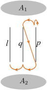
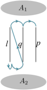
Figure 1: Two glasma superdiagrams to determine the rapidity indices of UGDs in Eqs. (2) and (3). The superdiagram on the left produces the rapidity indices of the UGDs in ${\cal T}_{1}$ [see Eq. (2)] whereas the superdiagram on the right is for ${\cal T}_{2}$ [see Eq. (3)]. Whether one begins writing down UGDs starting from $A_{1}$ (left figure) or $A_{2}$ (right figure), the first UGD is always squared, which is $\Phi_{1,p}^{2}$ when one starts from $A_{1}$ and $\Phi_{2,l}^{2}$ when one starts from $A_{2}$. $C_{3}$ contains multiplication of three UGDs from $A_{1}$ and another three from $A_{2}$. In the superdiagram on the left, three hoppings on $A_{1}$ already brings three UGDs, so before reaching $l$, one has to move to the other nucleus. Another rule of the superdiagrams is that one starts from the rightmost index on $A_{1}$ ($p$) and ends at the leftmost index on $A_{2}$ as in the left superdiagram. There is also the same number of superdiagrams where one starts from the leftmost index on $A_{2}$ and end at the rightmost index on $A_{1}$ as in the right superdiagram. Since these two sets of superdiagrams are simultaneous horizontal and vertical reflections of each other, in the following figures we will only draw the first set of the superdiagrams where one start from the rightmost index on $A_{1}$. As for the hoppings, only next-to-nearing hoppings are allowed; hence, connecting $p$ to $l$ by skipping $q$ is not allowed.

The quadruple-gluon cumulant that requires calculation of 96 glasma diagrams can be produced with 4 superdiagrams. The fourth cumulant is given by Ozonder:2014sra

$$C_{4}(\bm{p},\bm{q},\bm{l},\bm{w})=\frac{\alpha_{s}^{4}N_{c}^{4}S_{\perp}}{\pi^{16}(N_{c}^{2}-1)^{7}}\frac{1}{\bm{p}_{\perp}^{2}\bm{q}_{\perp}^{2}\bm{l}_{\perp}^{2}\bm{w}_{\perp}^{2}}\int\frac{d^{2}\bm{k}_{\perp}^{2}}{(2\pi)^{2}}({\cal Q}_{1}+{\cal Q}_{2}),$$ (5)

where

$${\cal Q}_{1} = \Phi_{1,p}^{2}(\bm{k}_{\perp})\Phi_{1,q}(\bm{k}_{\perp})[4\times\Phi_{1,l}(\bm{k}_{\perp})+2\times\Phi_{1,q}(\bm{k}_{\perp})]\Phi_{2,p}(\bm{p}_{\perp}-\bm{k}_{\perp}){\cal Q}_{A_{2}},$$ (6)

$${\cal Q}_{2} = \Phi_{2,w}^{2}(\bm{k}_{\perp})\Phi_{2,l}(\bm{k}_{\perp})[4\times\Phi_{2,q}(\bm{k}_{\perp})+2\times\Phi_{2,l}(\bm{k}_{\perp})]\Phi_{1,p}(\bm{p}_{\perp}-\bm{k}_{\perp}){\cal Q}_{A_{1}},$$ (7)

$${\cal Q}_{A_{1}(A_{2})} = [\Phi_{1(2),q}(\bm{q}_{\perp}-\bm{k}_{\perp})+\Phi_{1(2),q}(\bm{q}_{\perp}+\bm{k}_{\perp})][\Phi_{1(2),l}(\bm{l}_{\perp}-\bm{k}_{\perp})+\Phi_{1(2),l}(\bm{l}_{\perp}+\bm{k}_{\perp})]$$ (8)

$$\,\,\,\times[\Phi_{1(2),w}(\bm{w}_{\perp}-\bm{k}_{\perp})+\Phi_{1(2),w}(\bm{w}_{\perp}+\bm{k}_{\perp})].$$

Fig. 2 shows the two superdiagrams that contributes to ${\cal Q}_{1}$; the two mirror images of these contractions (not shown in the figure) gives ${\cal Q}_{2}$.

‘

Figure 2: Two glasma superdiagrams that contribute to ${\cal Q}_{1}$ given in Eq. (6), which is part of $C_{4}$. The other two superdiagrams are not shown as they are simultaneous horizontal and vertical reflections of these two superdiagrams.

III RULES FOR SUPERDIAGRAMS

The rules of superdiagrams can be summarized as follows.

1. On nucleus $A_{1}$ ($A_{2}$), one starts from the rightmost (leftmost) rapidity index, and end at the leftmost (rightmost) rapidity index on $A_{2}$ ($A_{1}$). The first rapidity site is always visited twice; it is the rightmost (leftmost) site on $A_{1}$ ($A_{2}$).

2. For $C_{n}$, only $n$ hoppings are allowed on each nucleus. For example, there are four hoppings on $A_{1}$ for $C_{4}$ as shown in Fig. 2. Also, the line connecting the rapidity sites should continue by visiting nearest-neighbors without skipping any site. For example, going from $p$ directly to $l$ by skipping $q$ is not allowed.

3. Each site can only be visited twice at maximum.

In light of these rules, one can draw the possible 6 superdiagrams for $C_{5}$. Figure 3 shows three of these superdiagrams.

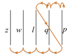
Figure 3: Three glasma superdiagrams that contribute to $C_{5}$. The other three superdiagrams are not shown as they are simultaneous horizontal and vertical reflections of these three superdiagrams.

Now a multi-gluon cumulant at any order for $n\geq 4$ can be constructed by the following recipe.

1. The prefactor and the integral part of $C_{n}$ shall be in the form

   $$C_{n}=\frac{\alpha_{s}^{n}N_{c}^{n}S_{\perp}}{\pi^{4n}(N_{c}^{2}-1)^{2n-1}}\left(\prod_{i=1}^{n}\frac{1}{\bm{p}_{\perp i}^{2}}\right)\int\frac{d^{2}\bm{k}_{\perp}^{2}}{(2\pi)^{2}}\left({\cal N}_{1}+{\cal N}_{2}\right).$$ (9)

2. ${\cal N}_{1}$ is given by

   $${\cal N}_{1}=\Phi_{1,p_{1}}^{2}(\bm{k}_{\perp})\left[\prod_{j=1}^{n-3}\Phi_{1,p_{j+1}}^{2}(\bm{k}_{\perp})\right]\left[\sum_{h=1}^{n-2}2^{h}\Phi_{1,p_{h+1}}^{2}(\bm{k}_{\perp})\right]\Phi_{2,p_{n}}(\bm{p}_{\perp 1}-\bm{k}_{\perp}){\cal N}_{A_{2}}.$$ (10)

   ${\cal N}_{2}$ can be obtained from ${\cal N}_{1}$ by making these changes: Replace the nucleus index 1 with 2, and replace the momentum index $p_{i}$ with $p_{n+1-i}$, where $n$ is the order of the cumulant. For example, one should change the indices according to $p\leftrightarrow w$ and $q\leftrightarrow l$ for $C_{4}$.

3. ${\cal N}_{A_{1}(A_{2})}$ that is contained in ${\cal N}_{2(1)}$ is given by

   $${\cal N}_{A_{1}(A_{2})}=\prod_{m=2}^{n}[\Phi_{1(2),p_{m}}(\bm{p}_{\perp m}-\bm{k}_{\perp})+\Phi_{1(2),p_{m}}(\bm{p}_{\perp m}+\bm{k}_{\perp})],$$ (11)

   where $n$ is again the order of the cumulant $C_{n}$. For $C_{4}$, $(p_{2},p_{3},p_{4})=(q,l,w)$, and $(\bm{p}_{\perp 2},\bm{p}_{\perp 3},\bm{p}_{\perp 4})=(\bm{q}_{\perp},\bm{l}_{\perp},\bm{w}_{\perp})$. [see Eq. (8)].

Equation (9) together with the definitions given in Eqs. (10) and (11) is the main result of this paper. $C_{n}$ gives inclusive $n$-gluon distribution, and it quantifies the correlation of $n$-gluons in transverse momentum and rapidity. $C_{n}$ can be used to calculate higher-dimensional ridges and flow moments $v_{m}(n\text{PC})$ from $n$-particle correlations. In principle, the cumulants $C_{n}$ can be summed to find the cumulant generating function, and then the probability distribution via Laplace transform of this generating function. We will not make any attempt in this direction since the UGDs contained in $C_{n}$ are complicated functions, and in practice they are in the form of numerical tables.

Now we shall check if the recipe given above yields the correct number of glasma diagrams for $C_{5}$. At the order $n=5$, ${\cal N}_{A_{2}}$ will contain $2^{4}$ separate terms, so ${\cal N}_{1}$ will contain $(2^{3}+2^{2}+2)\times 2^{4}=224$ terms. ${\cal N}_{2}$ contains the same number of diagrams, so the total number of connected diagrams becomes $448$. We shall now check if the cumulant expansion gives the same number of diagrams. The fifth cumulant $\kappa_{5}$, which is same as $C_{5}$, is given by in terms of the lower-order cumulants and the fifth moment $\mu_{5}$

$$\kappa_{5}=\mu_{5}-5\kappa_{4}\kappa_{1}-10\kappa_{3}\kappa_{2}-10\kappa_{3}\kappa_{1}^{2}-15\kappa_{2}^{2}\kappa_{1}-10\kappa_{2}\kappa_{1}^{3}-\kappa_{1}^{5}.$$ (12)

Here $\mu_{5}$ includes all connected and disconnected glasma rainbow diagrams with five gluons. Subtracting from $\mu_{5}$ the other terms in RHS of Eq. (12) gives the connected five gluon diagrams, which is $\kappa_{5}$. A word of caution regarding the term $\kappa_{2}^{2}$ is in order Ozonder:2014sra . $\kappa_{2}$ includes two upper and two lower rainbow diagrams. However, the term $\kappa_{2}^{2}$ mixes upper and lower rainbow diagrams. Such mixings do not occur in $\mu_{5}$, where the disconnected diagrams are formed either by the combination of lower or upper rainbow diagrams. So, since $\mu_{5}$ is already free from mixed diagrams, subtracting any mixed diagrams from $\mu_{5}$ would result in wrong counting. We resolve this issue by modifying the term in Eq. (12) as such

$$15\kappa_{2}^{2}\kappa_{1}\longrightarrow\frac{1}{2}15\kappa_{2}^{2}\kappa_{1},$$ (13)

so that only the diagrams of the form $\text{upper}\otimes\text{upper}$ and $\text{lower}\otimes\text{lower}$ are substracted from $\mu_{5}$, but not those of the form $\text{lower}\otimes\text{upper}$ or $\text{upper}\otimes\text{lower}$.

The fifth moment $\mu_{5}$ includes all connected and disconnected rainbow glasma diagrams at the five gluon level, and the number of such diagrams is given by $2(2n-1)!!-1$ Ozonder:2014sra . The first factor of 2 accounts for both upper and lower rainbow diagrams, the term with the double factorial counts the number of pairings between gluons, and 1 is subtracted at the end not to double count the maximally disconnected glasma diagram ($\kappa_{1}^{n}$), which is shown as concentric circles Ozonder:2014sra . At the order $n=5$, there are $\mu_{5}=1889$ connected and disconnected rainbow diagrams in total. The numbers of diagrams that each cumulant for $n<5$ contains have been given in Ref. Ozonder:2014sra : $\kappa_{1}=1$, $\kappa_{2}=4$, $\kappa_{3}=16$ and $\kappa_{4}=96$. From Eq. (12) with the modification in Eq. (13), we find the number of connected diagrams for $C_{5}$

$$\kappa_{5} = 1889-5\times 96-10\times 16\times 4-10\times 16$$ (14)

$$\,\,\,-15\times\frac{1}{2}\times 4^{2}-10\times 4-1=448.$$

This number is the same as what our recipe previously gave; see the discussion above Eq. (12). This completes the proof that our formulas given in the recipe Eqs. (9-11) produce the correct number of diagrams.

IV Summary and Outlook

We have developed a superdiagramatic technique which allows calculating the inclusive gluon distributions $C_{n}$ at the saturation limit easily bypassing the necessity of calculating thousands of glasma diagrams. Inclusive gluon distribution functions contain information on azimuthal and rapidity correlations between produced gluons in p-p, p-A and A-A collisions. Multiple-hadron correlations are measured in these experiments. These hadronic correlation functions are used to measure the ridge-type azimuthal correlations between hadrons as well as flow moments $v_{m}(n\text{PC})$ from multiple hadrons. On the theory side, hadron correlations are calculated by convolving the gluon correlation functions $C_{n}$ with fragmentation functions. Higher dimensional ridges from number of gluons $n>2$ and flow moments $v_{m}$ from multi-particle correlations are a testing ground for different approaches such as hydrodynamics and gluon saturation/glasma physics.

V Acknowledgments

This work is supported in part by U.S. Department of Energy Grant No. DE-FG02-00ER41132. For fruitful discussions, we thank Jean-Yves Ollitrault, Matthew Luzum, Wei Li and other participants of the INT Program INT 15-2b Correlations and Fluctuations in p+A and A+A Collisions.

References

- [1] Theodore Koblesky. Collectivity in Small QCD Systems. In 12th Conference on the Intersections of Particle and Nuclear Physics (CIPANP 2015) Vail, Colorado, USA, May 19-24, 2015, 2015.
- [2] Vardan Khachatryan et al. Observation of Long-Range Near-Side Angular Correlations in Proton-Proton Collisions at the LHC. JHEP, 1009:091, 2010.
- [3] Drago Velicanu. Ridge correlation structure in high multiplicity pp collisions with CMS. J.Phys., G38:124051, 2011.
- [4] Wei Li. Observation of a ’Ridge’ correlation structure in high multiplicity proton-proton collisions: A brief review. Mod.Phys.Lett., A27:1230018, 2012.
- [5] Serguei Chatrchyan et al. Observation of long-range near-side angular correlations in proton-lead collisions at the LHC. Phys.Lett., B718:795–814, 2013.
- [6] Serguei Chatrchyan et al. Multiplicity and transverse momentum dependence of two- and four-particle correlations in pPb and PbPb collisions. Phys. Lett., B724:213–240, 2013.
- [7] Betty Abelev et al. Long-range angular correlations on the near and away side in -Pb collisions at TeV. Phys.Lett., B719:29–41, 2013.
- [8] Georges Aad et al. Observation of Associated Near-side and Away-side Long-range Correlations in TeV Proton-lead Collisions with the ATLAS Detector. Phys.Rev.Lett., 110:182302, 2013.
- [9] Leonardo Milano. Long-range angular correlations at the LHC with ALICE. Nucl. Phys., A931:1017–1021, 2014.
- [10] Betty Bezverkhny Abelev et al. Long-range angular correlations of pi, K and p in p–Pb collisions at TeV. Phys.Lett., B726:164–177, 2013.
- [11] Betty Bezverkhny Abelev et al. Multiparticle azimuthal correlations in p -Pb and Pb-Pb collisions at the CERN Large Hadron Collider. Phys. Rev., C90(5):054901, 2014.
- [12] Betty Bezverkhny Abelev et al. Multiplicity dependence of jet-like two-particle correlation structures in p?Pb collisions at =5.02 TeV. Phys. Lett., B741:38–50, 2015.
- [13] Georges Aad et al. Measurement of long-range pseudorapidity correlations and azimuthal harmonics in TeV proton-lead collisions with the ATLAS detector. Phys. Rev., C90(4):044906, 2014.
- [14] Quan Wang. Azimuthal anisotropy of charged particles from multiparticle correlations in pPb and PbPb collisions with CMS. Nucl. Phys., A931:997–1001, 2014.
- [15] Alice Ohlson. Recent results on two-particle correlations in ALICE. J. Phys. Conf. Ser., 668(1):012074, 2016.
- [16] Vardan Khachatryan et al. Measurement of long-range near-side two-particle angular correlations in pp collisions at = 13 TeV. 2015.
- [17] Vardan Khachatryan et al. Evidence for Collective Multiparticle Correlations in p-Pb Collisions. Phys. Rev. Lett., 115(1):012301, 2015.
- [18] Piotr Bozek. Collective flow in p-Pb and d-Pd collisions at TeV energies. Phys.Rev., C85:014911, 2012.
- [19] Piotr Bozek. Elliptic flow in proton-proton collisions at TeV. Eur.Phys.J., C71:1530, 2011.
- [20] Piotr Bozek and Wojciech Broniowski. Correlations from hydrodynamic flow in p-Pb collisions. Phys.Lett., B718:1557–1561, 2013.
- [21] Igor Kozlov, Matthew Luzum, Gabriel Denicol, Sangyong Jeon, and Charles Gale. Transverse momentum structure of pair correlations as a signature of collective behavior in small collision systems. 2014.
- [22] Piotr Bozek, Wojciech Broniowski, and Adam Olszewski. Two-particle correlations in pseudorapidity in a hydrodynamic model. Phys. Rev., C92(5):054913, 2015.
- [23] Adam Bzdak and Piotr Bozek. Multi-particle long-range rapidity correlations from fluctuation of the fireball longitudinal shape. Phys. Rev., C93:024903, 2016.
- [24] Adrian Dumitru, Kevin Dusling, Francois Gelis, Jamal Jalilian-Marian, Tuomas Lappi, et al. The Ridge in proton-proton collisions at the LHC. Phys.Lett., B697:21–25, 2011.
- [25] Kevin Dusling and Raju Venugopalan. Azimuthal collimation of long range rapidity correlations by strong color fields in high multiplicity hadron-hadron collisions. Phys.Rev.Lett., 108:262001, 2012.
- [26] Kevin Dusling and Raju Venugopalan. Evidence for BFKL and saturation dynamics from dihadron spectra at the LHC. Phys.Rev., D87(5):051502, 2013.
- [27] Kevin Dusling and Raju Venugopalan. Explanation of systematics of CMS p+Pb high multiplicity di-hadron data at TeV. Phys.Rev., D87(5):054014, 2013.
- [28] Kevin Dusling and Raju Venugopalan. Comparison of the color glass condensate to dihadron correlations in proton-proton and proton-nucleus collisions. Phys.Rev., D87(9):094034, 2013.
- [29] F. Gelis, T. Lappi, and L. McLerran. Glittering Glasmas. Nucl.Phys., A828:149–160, 2009.
- [30] Sener Ozonder. Triple-gluon and quadruple-gluon azimuthal correlations from glasma and higher-dimensional ridges. Phys.Rev., D91(3):034005, 2015.
- [31] Adrian Dumitru, Tuomas Lappi, and Larry McLerran. Are the angular correlations in collisions due to a Glasmion or Bose condensation? Nucl. Phys., A922:140–149, 2014.
- [32] Adam Bzdak, Piotr Bozek, and Larry McLerran. Fluctuation induced equality of multi-particle eccentricities for four or more particles. Nucl. Phys., A927:15–23, 2014.
- [33] Adrian Dumitru, Francois Gelis, Larry McLerran, and Raju Venugopalan. Glasma flux tubes and the near side ridge phenomenon at RHIC. Nucl.Phys., A810:91–108, 2008.
- [34] Larry D. McLerran and Raju Venugopalan. Computing quark and gluon distribution functions for very large nuclei. Phys.Rev., D49:2233–2241, 1994.
- [35] Larry D. McLerran and Raju Venugopalan. Gluon distribution functions for very large nuclei at small transverse momentum. Phys.Rev., D49:3352–3355, 1994.
- [36] Larry D. McLerran and Raju Venugopalan. Green’s functions in the color field of a large nucleus. Phys.Rev., D50:2225–2233, 1994.
- [37] Yuri V. Kovchegov. NonAbelian Weizsacker-Williams field and a two-dimensional effective color charge density for a very large nucleus. Phys.Rev., D54:5463–5469, 1996.
- [38] Sener Ozonder. Determination of the Parameters of a Color Neutral 3D Color Glass Condensate Model. Phys.Rev., D87(4):045013, 2013.
- [39] Kevin Dusling, Francois Gelis, Tuomas Lappi, and Raju Venugopalan. Long range two-particle rapidity correlations in A+A collisions from high energy QCD evolution. Nucl.Phys., A836:159–182, 2010.