A Stochastic Performance Model for Pipelined Krylov Methods

Abstract

Pipelined Krylov methods seek to ameliorate the latency due to inner products necessary for projection by overlapping it with the computation associated with sparse matrix-vector multiplication. We clarify a folk theorem that this can only result in a speedup of $2\times$ over the naive implementation. Examining many repeated runs, we show that stochastic noise also contributes to the latency, and we model this using an analytical probability distribution. Our analysis shows that speedups greater than $2\times$ are possible with these algorithms.

KEY WORDS: asynchronous; pipelined; Krylov; stochastic; PGMRES; PIPECG; split phase collective; performance model

1 Introduction

Krylov methods [1] have become an indispensible tool for the scalable solution of large, sparse linear systems, which in turn have enabled an explosion in massively parallel scientific simulation [2]. However, as we move to larger massively parallel architectures, the latency cost for reduction operations, central to Krylov methods, has ballooned [3]. In an effort to control these costs, “pipelined” versions of many Krylov algorithms have been developed, which allow some of the latency cost to be hidden by computational work.

A pipelined version of the classical CG method was already developed in [4] for vector machines, revisited for large scale parallelism in [5], and implemented for field-programmable gate arrays in [6]. Similarly, pipelined versions of CG [7], GMRES [8] and BiCGStab [9] have also been put forward. One cannot arbitrarily remove synchronizations from algorithms and expect comparable behavior, so pipelined variants of Krylov methods employ rearrangements which give arithmetically equivalent methods with looser data dependencies and the possibility to overlap computation and global communication, at the cost of additional intermediate storage and local computation, increased latency as a pipeline is filled, and degraded numerical stability. We have included a GMRES algorithm (Algorithm 1) and a pipelined version by [8] (Algorithm 2) below for completeness.

Algorithm 1 GMRES

1:$r_{0}\leftarrow b-Ax_{0}$; $v_{0}\leftarrow r_{0}/\|r_{0}\|_{2}$

2:for $i=0,1,\dots,m-1$ do

3:     $z\leftarrow Av_{i}$

4:     $h_{j,i}\leftarrow\langle z,v_{j}\rangle,j=0,1,\dots,i$

5:     $\tilde{v}_{i+1}\leftarrow z-\sum_{j=1}^{i}h_{j,i}v_{j}$

6:     $h_{i+1,i}\leftarrow\|\tilde{v}_{i+1}\|_{2}$

7:     $v_{i+1}\leftarrow\tilde{v}_{i+1}/h_{i+1,i}$

8:     # apply Givens rotations to $H_{:,i}$

9:end for

10:$y_{m}\leftarrow\text{argmin}\|(H_{m+1,m}y_{m}-\|r_{0}\|_{2}e_{1})\|_{2}$

11:$x\leftarrow x_{0}+V_{m}y_{m}$

Algorithm 2 PGMRES

1:$r_{0}\leftarrow b-Ax_{0}$; $v_{0}\leftarrow r_{0}/\|r_{0}\|_{2}$; $z_{0}\leftarrow v_{0}$

2:for $i=0,1,\dots,m+1$ do

3:     $w\leftarrow Az_{i}$

4:     if i $>$ 1 then

5:         $v_{i-1}\leftarrow v_{i-1}/h_{i-1,i-2}$

6:         $z_{i}\leftarrow z_{i}/h_{i-1,i-2}$

7:         $w\leftarrow w/h_{i-1,i-2}$

8:         for $j=0,1,\dots,i$ do

9:              $h_{j,i-1}\leftarrow h_{j,i-1}/h_{i-1,i-2}$

10:         end for

11:         $h_{i-1,i-1}\leftarrow h_{i-1,i-1}/h^{2}_{i-1,i-2}$

12:     end if

13:     $z_{i+1}\leftarrow w-\sum_{j=0}^{i-1}h_{j,i-1}z_{j+1}$

14:     if i $>$ 0 then

15:         $v_{i}\leftarrow z_{i}-\sum_{j=0}^{i-1}h_{j,i-1}v_{j}$

16:         $h_{i,i-1}\leftarrow\|v_{i}\|_{2}$

17:     end if

18:     $h_{j,i}\leftarrow\langle z_{i+1},v_{j}\rangle,j=0,1,\dots,i$

19:end for

20:$y_{m}\leftarrow\text{argmin}\|(H_{m+1,m}y_{m}-\|r_{0}\|_{2}e_{1})\|_{2}$

21:$x\leftarrow x_{0}+V_{m}y_{m}$

It has been difficult to understand the performance of these solvers on existing machines, judge the impact of algorithmic tradeoffs, and predict performance on future architectures due to the lack of a coherent performance model [10]. For example, some runs in [5] exhibit a speedup of slightly more than a factor of 2, but this is difficult to explain in a deterministic model, as will be shown in Section 2.

In this work, we present a stochastic performance model for pipelined Krylov solvers, detailed in Section 2, and examine the implications of different waiting time distributions on algorithm performance in Section 3. These predictions are compared to parallel experiments in Section 4.

2 Mathematical Model

We model a Krylov iterative method as a set of $P$ communicating processes who must perform a calculation consisting of local computations, separated by periodic global synchronizations, and interrupted by waiting, perhaps due to unsatisfied requests to memory, actions of the operating system, etc. We will label the set of computations and waiting by the index $k$, which corresponds to the iteration number for the Krylov method. The removal of the global synchronizations will correspond to the introduction of split-phase collectives [10] for the norm calculation and orthogonalization step. A split-phase, or non-blocking, collective is a collective operation, such as a broadcast, which has been split into two parts so that it no longer requires a global synchronization at the point of the call. Rather, the collective operation is first initiated, say with MPI_Ibcast(), and then later finalized with MPI_Wait(). This strategy removes the global synchronization and allows the operation to be overlapped with useful work between the initialization and finalization. The ratio between times with and without synchronization will give us a bound on the speedup of the pipelined algorithm over the classical variant. Below we illustrate this model using $P=2$ processes.

2.1 Deterministic Computation and Waiting Times

In the simplest scenario, each process takes a certain time $c_{p}$ for local computation, $w_{p}$ for waiting, which is independent of the step $k$. Fig. 1 represents computation with three steps.

Figure 1: Computation with $P=2$ processes for $K=3$ steps. The green rectangles represent computation, the purple waiting, and the dotted lines are synchronization.

The total running time $T$, or makespan, of the computation is then given by the expression

$$T=\sum_{k}\max_{p}(c_{p}+w_{p})=K\,\max_{p}T_{p},$$ (1)

where $K$ is the total number of steps, and $T_{p}=c_{p}+w_{p}$ is the time on process $p$ for one step excluding waiting for the global barrier. Clearly, without loss of generality, we can replace the separate computation and waiting timing with a single process time $T_{p}$.

If we remove the synchronizations, as shown in Fig. 2,

Figure 2: Computation with $P=2$ processes for $K=3$ steps. The green rectangles represent computation, the purple waiting, and there is no synchronization.

then the makespan is given by

$$T^{\prime}=\max_{p}\sum_{k}(c_{p}+w_{p})=K\max_{p}T_{p},$$ (2)

so that no speedup is achievable. The removal of synchronizations can in general be modeled by the interchange of the sum over steps and the maximum over process times.

2.2 Stochastic Process Times

If we allow the amount of local computation and waiting to fluctuate over the steps, as shown in Fig. 3, we will see that speedup is achievable, as shown in Fig. 4. Most simulation codes, including most linear solvers, statically partition the data so that computation times do not show large fluctuations. Waiting times, however, are more volatile and fluctuate across processes and steps [11], which can arise from interactions with the OS [12].

In the very simple scenario that one process waits for a long time $W$ on the first step, the other on the second, and on other steps the processes both take time $T_{0}$, as shown in Fig. 3,

Figure 3: Computation with $P=2$ processes for $K=5$ steps. The green rectangles represent computation, the purple waiting, and the dotted lines are synchronization.

Figure 4: Computation with $P=2$ processes for $K=5$ steps. The green rectangles represent computation, the purple waiting, and there is no synchronization.

then the makespan with and without synchronizations is given by

$$T =\sum_{k}\max_{p}T_{p}=2W+KT_{0},$$ (3)

$$T^{\prime} =\max_{p}\sum_{k}T_{p}=W+KT_{0}.$$ (4)

Thus the possible speedup is

$$\frac{T}{T^{\prime}}=\frac{2W+KT_{0}}{W+KT_{0}}=\frac{2+\alpha}{1+\alpha}$$ (5)

where $\alpha=KT_{0}/W$, which is bounded above by 2. Extended to $P$ processes this gives an upper bound of $P$ on the speedup, since all the waiting time is collapsed to the first interval when synchronization is removed and computation time becomes small. This is related to the folklore result that speedup from covering communication with computation is limited to a factor of 2, where we have two players, computing and communicating. This is because if we cover all communication by computation, then one is larger than the other and is more than half of the computational time.

3 Stochastic Model

We will employ a stochastic description of the waiting time variation making it amenable to analysis. We begin with a stochastic process time $\mathcal{T}^{k}_{p}$ at each step that is drawn from a distribution independent of process and stationary in step number. Let $T$ be the total Krylov time (computation and waiting) of the classical algorithm with synchronization, and $T^{\prime}$ the total time for the pipelined version without synchronization where $T=\sum_{k}\max_{p}\mathcal{T}^{k}_{p}$ and $T^{\prime}=\max_{p}\sum_{k}\mathcal{T}^{k}_{p}$. We can ask for the expected total time with and without synchronizations,

$$E[T]=E[\sum_{k}\max_{p}\mathcal{T}^{k}_{p}]=\sum_{k}E[\max_{p}\mathcal{T}^{k}_{p}],$$ (6)

and

$$E[T^{\prime}]=E[\max_{p}\sum_{k}\mathcal{T}^{k}_{p}].$$ (7)

These stage times will be modeled as random variables, drawn from some underlying distribution. Since the time spent computing should not fluctuate, within our measurement accuracy, it only affects the mean of the distribution. The variability in the distribution models the waiting times which can arise from interactions with the OS [11, 12]. We assume that waiting times across processes are independent because we have no expectation that OS operations will be correlated across processes. In this section, we compute the ratio of these quantities for a range of representative distributions for waiting times, in order to estimate the potential speedup.

3.1 Formulation

We would like to calculate the speedup after $k$ steps, $\frac{E[T]}{E[T^{\prime}]}$, where expected total time $E[T]$ is defined by (6) and likewise $E[T^{\prime}]$ is defined by (7). First, we will derive an expression for the expected value of the maximum of a set of random variables in order to find an expression for $E[T]$. Then we will find one for $E[T^{\prime}]$.

A general expression for the expected value of the maximum of a set of random variables can be found in [13] and is described here for completeness. Let $X_{1},X_{2},\dots,X_{n}$ be independent, identically distributed (iid) random variables with probability distribution function (pdf) $f(x)$ and cumulative distribution function (cdf) $F(x)$. Let $X_{\max}$ be another random variable such that $X_{\max}=\max\{X_{1},X_{2},\dots,X_{n}\}$. By noticing that $X_{\max}\leq x$ if and only if $X_{i}\leq x$ for all $i$’s,

$$F_{\max}(x) =P(X_{\max}\leq x)$$

$$=P(X_{1}\leq x,X_{2}\leq x,\dots,X_{n}\leq x)$$

$$=P(X_{1}\leq x)P(X_{2}\leq x)\dots P(X_{n}\leq x)$$

$$=F(x)F(x)\dots F(x)$$

$$=F(x)^{n}$$

using the fact that the $X_{i}$’s are independent and identically distributed. Furthermore,

$$f_{\max}(x)=\frac{d}{dx}F_{\max}(x)=\frac{d}{dx}F(x)^{n}=nF(x)^{n-1}f(x)$$

since by definition $\frac{d}{dx}F(x)=f(x)$. The expected value of $X_{\max}$, integrating over the support of $x$, is

$$E[X_{\max}]=n\int^{\infty}_{-\infty}xF(x)^{n-1}f(x)dx.$$ (8)

At step $k=1$, we have $P$ iid random variables $\mathcal{T}^{1}_{0},\mathcal{T}^{1}_{1},\dots,\mathcal{T}^{1}_{P-1}$ from an underlying distribution with pdf $f_{1}(x)$, cdf $F_{1}(x)$, and joint cdf $F(x_{0},x_{1},\dots,x_{P-1})$. Similarly, for a given step $k$, $\mathcal{T}^{k}_{0},\mathcal{T}^{k}_{1},\dots,\mathcal{T}^{k}_{P-1}$ are iid random variables with pdf $f_{k}(x)$, cdf $F_{k}(x)$, and joint cdf $F(x_{0},x_{1},\dots,x_{P-1})$. Since the random variables are stationary in $k$, the joint cdf and thus the individual pdfs and cdfs remain the same at step $k$ so that $f_{1}(x)=f_{k}(x)$ and $F_{1}(x)=F_{k}(x)$. Then using (8), we have

$$E[\max_{p}\mathcal{T}^{1}_{p}]=P\int^{\infty}_{-\infty}xF_{1}(x)^{P-1}f_{1}(x)dx=E[\max_{p}\mathcal{T}^{k}_{p}].$$

Then

$$E[T]=\sum_{k}E[\max_{p}\mathcal{T}^{k}_{p}]=KE[\max_{p}\mathcal{T}^{1}_{p}].$$

Also because the random variables $\mathcal{T}^{k}_{p}$ are stationary in $k$, $E[\mathcal{T}^{k}_{p}]=\mu$ for all $k$. The sum $\sum_{k}\mathcal{T}^{k}_{p}$ will approach $K\mu$ in the limit of large $K$ so that we also have

$$E[T^{\prime}] =E\big{[}\max_{p}\sum_{k}\mathcal{T}^{k}_{p}\big{]}\to K\mu.$$

In this case, speedup is given by $\dfrac{E[T]}{E[T^{\prime}]}\to\dfrac{E[\max_{p}\mathcal{T}^{1}_{p}]}{\mu}$.

We will examine a of range of common analytical distributions. As the tails of $f_{k}(x)$ become heavier, the potential speedup increases and can eventually exceed $2\times$.

3.2 Uniform Distribution

Let the $\mathcal{T}_{p}$’s from $P$ processes be independent random variables from a uniform distribution on $[a,b]$ with pdf $f(x)=\frac{1}{b-a}$, cdf $F(x)=\frac{x-a}{b-a}$, and mean $\mu=\frac{a+b}{2}$. Using (8), we calculate the expected value of the maximum

$$E[\max_{p}\mathcal{T}_{p}] =P\int^{b}_{a}x\bigg{(}\frac{x-a}{b-a}\bigg{)}^{P-1}\frac{1}{b-a}dx$$

$$=\frac{a+Pb}{P+1}$$

to find speedup on $P$ processes

$$\frac{E[T]}{E[T^{\prime}]}=\dfrac{\dfrac{a+Pb}{P+1}}{\dfrac{a+b}{2}}=\frac{2(a+Pb)}{(P+1)(a+b)}.$$

On the interval $[0,b]$, we find that the asynchronous speedup, $\dfrac{2P}{P+1}$, is bounded from above by 2.

3.3 Exponential Distribution

Let $\mathcal{T}_{0},\mathcal{T}_{1},\mathcal{T}_{2},\mathcal{T}_{3}$, the times for four processes, be independent random variables from an exponential distribution with pdf $f(x)=\lambda e^{-\lambda x}$, cdf $F(x)=1-e^{-\lambda x}$, and mean $\mu=\frac{1}{\lambda}$. Again, using (8), we calculate the expected value of the maximum

$$E[\max_{p}\mathcal{T}_{p}] =4\lambda\int^{\infty}_{0}x\big{(}1-e^{-\lambda x}\big{)}^{3}e^{-\lambda x}dx$$

$$=\frac{25}{12\lambda}.$$

We find that the speedup on four processes is

$$\frac{E[T]}{E[T^{\prime}]}=\dfrac{25/12\lambda}{1/\lambda}=\frac{25}{12}>2.$$

When the $\mathcal{T}_{p}$’s are from an exponential distribution, asynchronous speedup is greater than 2 on four or more processes. Furthermore, the speedup on $P$ processes

$$\frac{E[T]}{E[T^{\prime}]}=\dfrac{E[\max_{p}\mathcal{T}_{p}]}{\mu}=\frac{\lambda P\int^{\infty}_{0}x\big{(}1-e^{-\lambda x}\big{)}^{P-1}e^{-\lambda x}dx}{1/\lambda}=H_{P}.$$

Here, $H_{P}=\log P+\gamma+O(1/P)$ is the $P$th harmonic number and $\gamma$ is Euler’s constant  [14].

3.4 Log-normal Distribution

Let the $\mathcal{T}_{p}$’s from $P$ processes be independent random variables from a log-normal distribution with pdf $f(x)=\frac{1}{x\sqrt{2\pi}\sigma}e^{\frac{-(\ln(x)-\mu)^{2}}{2\sigma^{2}}}$, cdf $F(x)=\frac{1}{2}+\frac{1}{2}\operatorname{erf}\big{(}\frac{\ln(x)-\mu}{\sqrt{2}\sigma}\big{)}$, and mean $\mu^{\prime}=e^{\mu+\frac{\sigma^{2}}{2}}$. Note that if a random variable $X$ is normally distributed with mean $\mu$ and variance $\sigma$, then $Y=e^{X}$ is a random variable from a log-normal distribution with mean $\mu^{\prime}$. After fixing $P$, $\mu$, and $\sigma$, we can calculate the speedup from $P$ processes numerically using equation (8) and Octave’s quad function. First, let $P=2$, $\mu=0$, and $\sigma=1$. Equation (8) becomes

$$E[\max_{p}\mathcal{T}_{p}]=2\int^{\infty}_{0}x\bigg{(}\frac{1}{2}+\frac{1}{2}\operatorname{erf}\bigg{(}\frac{\ln(x)}{\sqrt{2}}\bigg{)}\bigg{)}\bigg{(}\frac{1}{x\sqrt{2\pi}}e^{\frac{-(\ln(x))^{2}}{2}}\bigg{)}dx\approx 2.5069,$$

so that the speedup on two processes is

$$\frac{E[T]}{E[T^{\prime}]}=\dfrac{E[\max_{p}\mathcal{T}_{p}]}{\mu^{\prime}}\approx\frac{2.5069}{\sqrt{e}}\approx 1.5205.$$

Now let $P=4$, $\mu=0$, and $\sigma=1$. Equation (8) becomes

$$E[\max_{p}\mathcal{T}_{p}]=4\int^{\infty}_{0}x\bigg{(}\frac{1}{2}+\frac{1}{2}\operatorname{erf}\bigg{(}\frac{\ln(x)}{\sqrt{2}}\bigg{)}\bigg{)}^{3}\bigg{(}\frac{1}{x\sqrt{2\pi}}e^{\frac{-(\ln(x))^{2}}{2}}\bigg{)}dx\approx 3.6406.$$

We again find that on four processors, the potential speedup is greater than 2:

$$\frac{E[T]}{E[T^{\prime}]}\approx\frac{3.6406}{\sqrt{e}}\approx 2.2081>2.$$

4 Experimental Results

The speedups reported in [5] for PIPECG and PIPECR on an Intel Xeon cluster using Infiniband seem limited by $2\times$ speedup, but at the limit of 20 processes exceed this slightly (2.09 and 2.14 respectively). However, understanding the origin of speedup exceeding $2\times$ requires the examination of many identical runs in order to amass statistics. Thus, we have generated repeated runs for PETSc KSP tutorial ex23 using CG, PIPECG, GMRES, and PGMRES on 8192 processors of the Piz Daint Cray XC30 supercomputer at CSCS [15], storing the data in an open repository [16]. The PIPECG and PGMRES algorithms are similar in that work involving sparse matrix-vector products (SpMV) is juxtaposed with work involving vector dot products. The dot products are reductions which require some sort of global synchronization. Thus the computational portion of our model is associated to the SpMV and orthogonalization with the BLAS AXPY calls, whereas the synchronizations apply to the dot product portion. These algorithms decouple these two operations, so that as long as the SpMV is more expensive than a global synchronization, the dot product operation involves negligible waiting.

The ex23 tutorial uses a simple, tridiagonal system of size 2,097,152, which is a one-dimensional discretization of the Laplacian, and we force 5000 iterates of the Krylov method. The pipelined methods produce almost identical residuals to the original methods for this problem. Most of the runtime for CG and PIPECG is thus concentrated in dot products, the VecTDot() operation in PETSc, rather than in SpMV. This means there is no computation to cover the communication cost, and very often we see no speedup, or even slowdown, for these runs. In [5], PIPECG achieves $2\times$ speedup for SNES tutorial ex48 because the much denser matrices in ex48 provide enough computation to cover the communication costs. PETSc ex48 solves the hydrostatic, that is Blatter-Pattyn, equations for ice sheet flow, where the ice uses a power-law rheology with Glen exponent 3. This generates a much denser system of equations with about 10x more nonzeros per row than ex23. The GMRES and PGMRES runs are also constrained to use 5000 iterates, however here this generates considerable work in the orthogonalization phase. This is analogous to the situation with PIPECG for ex48, so it can be covered by the split collective, and we again see a roughly $2\times$ speedup. We note that an increase in the number of iterates is possible, but not observed in [8, 5] for the setup we use in this paper.

However, we also see some outliers in the data where speedup exceeds $2\times$. This could potentially be explained by assuming a noise distribution and using the prior results from Sec. 3. Thus, we would like to show that a set of observed random variables $X_{1},X_{2},\dots,X_{n}$ comes from some underlying distribution using well-known statistical tests. In our case, we want to fit two different sets of observations: the multiples of twelve (so that $n=12$) runs of a pipelined GMRES algorithm and twenty runtimes ($n=20$) of a pipelined CG algorithm. Both algorithms were run on 8192 processors on Piz Daint.

4.1 Cramér-von Mises

Let $X_{1},X_{2},\dots,X_{n}$ be $n$ observed values in increasing order and assume that $F(x)$ is the cdf of the underlying distribution. The Cramér-von Mises test statistic is given by

$$T=\frac{1}{12n}+\sum_{i=1}^{n}\bigg{[}\frac{2i-1}{2n}-F(X_{i})\bigg{]}^{2}$$ (9)

If $T$ is larger than a tabulated limit value, we reject our assumption that the observations came from the distribution with cdf $F(x)$. P-values for the test statistic can be found in [17] and critical values in [18]. We use a significance level $\alpha=0.05$ in all of our tests.

Using the Cramér-von Mises statistic, we look at the consistency of our observations with both uniform and exponential distributions. The cdfs are given by $F(x)=\frac{x-a}{b-a}$ over the support of $x$ and $F(x)=1-e^{(-\lambda x)}$ for $x>0$, respectively. The Cramér-von Mises test allows one to estimate the parameters of the distribution from the sample, unlike non-parametric tests such as Kolmogorov-Smirnov where the underlying distribution parameters are assumed to be known. In the case of the uniform distribution, we will let the parameters $a$ and $b$ be $X_{1}$ and $X_{n}$, the minimum and maximum observations and we will use maximum-likelihood estimation (MLE) to recover $\lambda$ for the exponential distribution, which in this case gives $\frac{1}{\lambda}=\frac{1}{n}\sum_{i=1}^{n}X_{i}$.

4.2 Lilliefors

The Lilliefors test is a normality test based on Kolmogorov-Smirnov where the expected value and the variance of the underlying distribution are not specified. We will use it to fit our observations to a log-normal distribution by first taking the natural logarithm of each sample $X_{1},X_{2},\dots,X_{n}$ and normalizing each sample so that

$$Z_{i}=\frac{\ln(X_{i})-(\bar{x})}{s}$$ (10)

where $\bar{x}$ is the sample mean and $s$ the sample standard deviation. The Lilliefors test statistic can then be calculated using

$$T=\sup\big{|}F(x)-S(x)\big{|}$$ (11)

where $F(x)$ is the standard normal cdf and $S(x)$ is the empirical distribution function for $Z_{1},Z_{2},\dots,Z_{n}$. Again, if the test statistic $T$ is larger than a tabulated critical value, we reject the hypothesis that the sample came from a normal distribution with significance level $\alpha$. Critical values can be found in [18] and we use the Matlab function lillietest to calculate $T$.

4.3 PGMRES and PIPECG

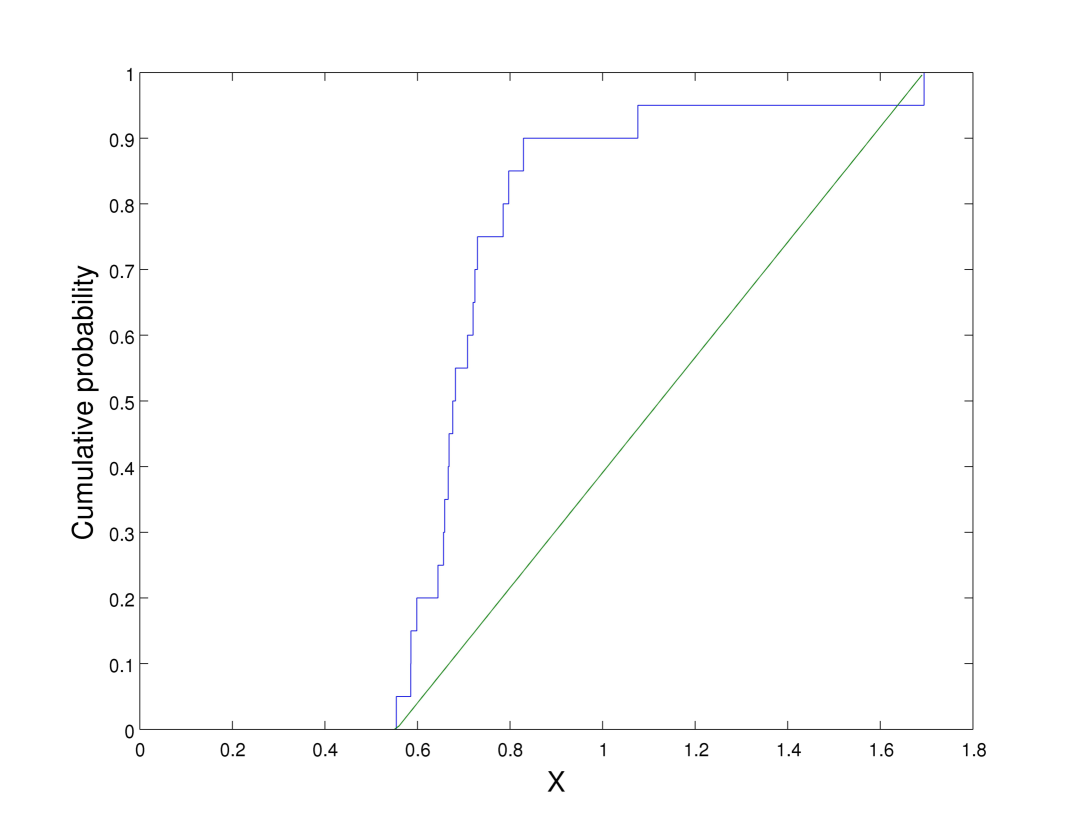
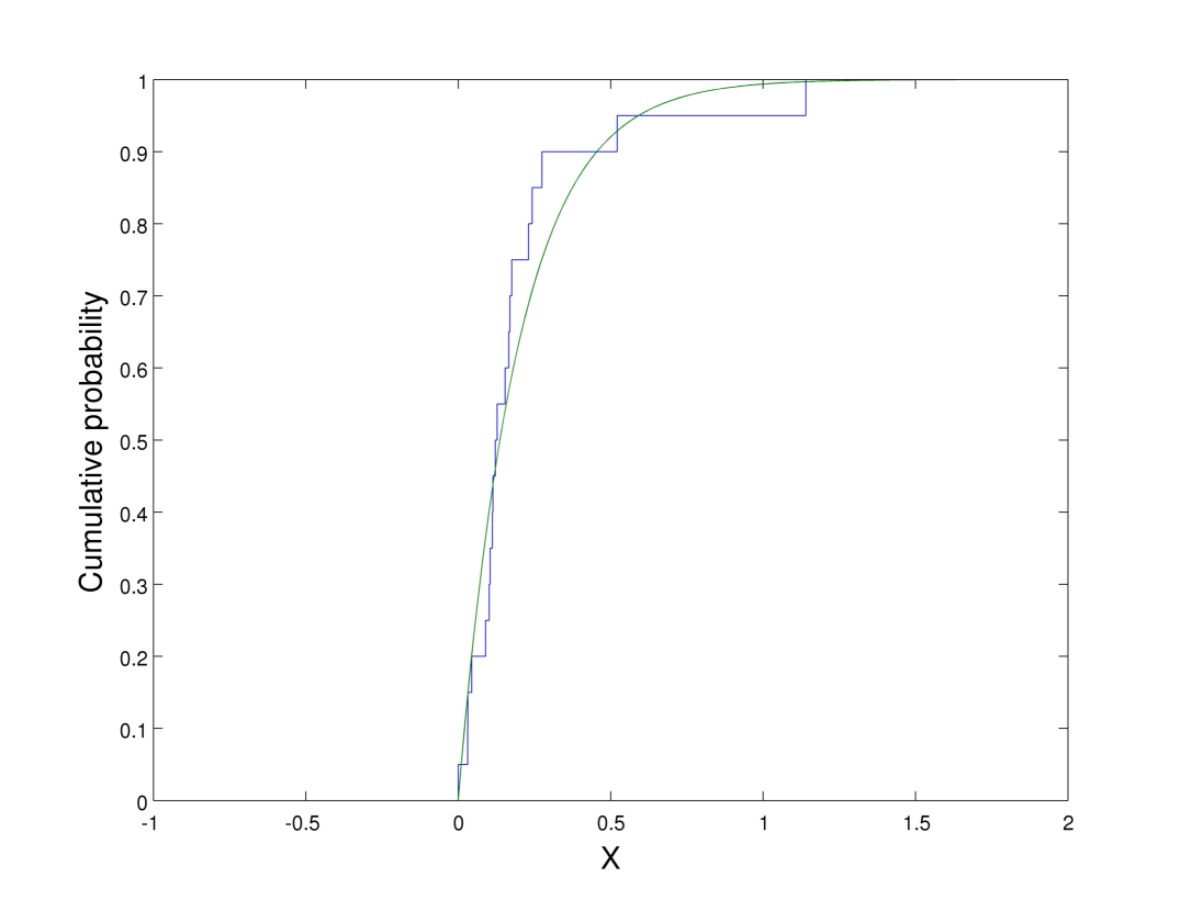
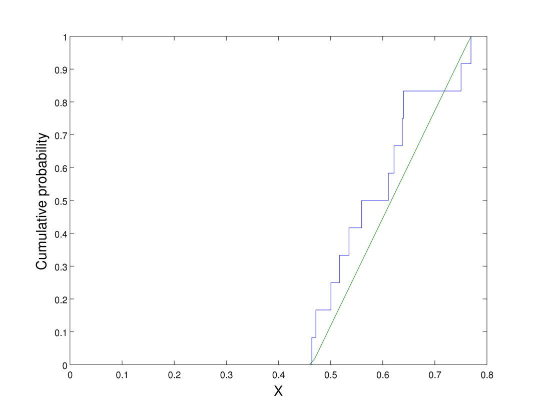
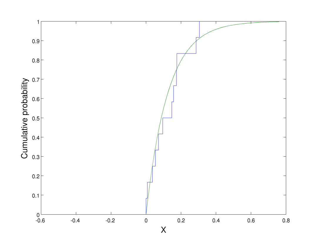
Summary statistics for the GMRES, PGMRES, CG, and PIPECG runs are given in Table 1, and the empirical cumulative distribution functions along with MLE proposed distributions are shown in Fig. 5 and 6.

Table 1: PGMRES and PIPECG runtime statistics

	GMRES	PGMRES	CG	PIPECG
$\bar{x}$	0.9465	0.5902	0.9349	0.7521
median	0.9932	0.5856	0.8632	0.6792
s	0.1303	0.0962	0.2385	0.2429
$\text{s}^{2}$	0.0170	0.0092	0.0569	0.0590
$\lambda$	1.0565	1.6942	1.0696	1.3295
$X_{\text{min}}$	0.6617	0.4644	0.6051	0.5545
$X_{\text{max}}$	1.0740	0.7697	1.6060	1.6950

Considering Fig. 5, with significance level $\alpha=0.05$, we reject the assumption that the PGMRES runtimes come from a uniform distribution, and clearly the data are quite far from uniform. Using the Cramér-von Mises statistic, we cannot reject the hypothesis that the distribution is exponential, nor can we reject a log-normal distribution using the Lilliefors test. Due to the small variation in the runs we cannot distinguish these alternatives with any confidence. More experiments must be run in order to obtain better statistics.

(a) Uniform Distribution

(b) Exponential Distribution

(c) Log-normal Distribution

Figure 5: We plot the empirical cumulative distribution for running times of PGMRES on PETSc KSP ex23, and also the MLE fit for analytic distributions, 5(a) uniform, 5(b) exponential, and 5(c) log-normal.

(a) Uniform Distribution

(b) Exponential Distribution

Figure 6: We plot the empirical cumulative distribution for running times of PIPECG on PETSc KSP ex23, and also the MLE fit for analytic distributions, 6(a) uniform, and 6(b) exponential.

Using the same methodology in Fig. 6, it is clear that the PIPECG runtimes are not uniform. Like PGMRES, most of the samples are clustered in a small range, but one outlier ran for over twice as long as the sample median. Using our tests, we reject that the runtimes come from uniform and log-normal distributions, but they are consistent with an exponential distribution.

It appears that some level of system noise is present in these simulations, since the exponential distribution provides a much better explanation for the data than a narrow uniform window, and this noise enables significant speedup when using the asynchronous Krylov methods. In Sec. 3 we showed that for exponentially distributed noise, speedup is given by

$$H_{P}=\sum_{i=1}^{P}\frac{1}{p}$$ (12)

on $P$ processors. Thus PIPECG could possibly attain speedup greater than 2 when $P\geq 4$, but it appears in practice that many more processors are necessary.

5 Conclusions

According to the performance data in publication dealing with asynchronous Krylov methods [5] that overall speedup did not exceed $2\times$, confirming the folk theorem for the case that we do no more than overlap communication with computation. However, looking at a large number of repeated runs, we find that operating system noise makes a measurable contribution, and can raise the speedup bound necessitating a new analysis. We show that uncommon delays, which could quite possibly have been rejected as outliers in other work, are well-modeled by an exponential distribution. Combined with our new analysis, this demonstrates that speedup greater than $2\times$ is possible for isolated runs, and in a statistical sense.

In future work, we will apply these algorithms to high latency situations where we expect unpredictable delays, such as heavily loaded machines, loosely coupled networks such as those employed for cloud computing or wireless computing clusters, and heterogeneous machines such as those using GPUs. These workloads must be seen in a statistical sense since most users will see computations contaminated by unpredictable, stochastic delays. Our analysis shows the effectiveness of asynchronous methods in these situations, the necessity of characterizing the distribution of noise, and can perhaps guide performance tuning of current algorithms and the development of new projection methods.

We also note that other potential sources of speedup have been identified. In [19], the authors show that pipelined solvers can be implemented on a GPU using fewer kernel launches. Since kernel launch incurs a significant latency penalty on the GPU, pipelined solvers can realize speedup from this fact alone.

References

- [1] Saad Y. Iterative Methods for Sparse Linear Systems, 2nd edition. SIAM: Philadelpha, PA, 2003.
- [2] Keyes DE ( (ed.)). A Science-based Case for Large-scale Simulation. U.S. Department of Energy, 2004. URL http://www.pnl.gov/scales.
- [3] Dongarra J, Luszczek P, et al.. HPC challenge 2015. URL http://icl.cs.utk.edu/hpcc/hpcc_results_lat_band.cgi?display=opt.
- [4] Chronopoulos AT, Gear CW. -step iterative methods for symmetric linear systems. Journal of Computational and Applied Mathematics 1989; 25:153–168.
- [5] Ghysels P, Vanroose W. Hiding global synchronization latency in the preconditioned conjugate gradient algorithm. Parallel Computing 2014; 40(7):224–238, doi:http://dx.doi.org/10.1016/j.parco.2013.06.001. URL http://www.sciencedirect.com/science/article/pii/S0167819113000719, 7th Workshop on Parallel Matrix Algorithms and Applications.
- [6] Strzodka R, Göddeke D. Pipelined mixed precision algorithms on FPGAs for fast and accurate PDE solvers from low precision components. Proceedings of the 14th Annual IEEE Symposium on Field-Programmable Custom Computing Machines, IEEE Computer Society, 2006; 259–270. FCCM ’06.
- [7] de Sturler E, van der Vorst H. Reducing the effect of global communication in GMRES(m) and CG on parallel distributed memory computers. Applied Numerical Mathematics 1995; 18(4):441–459.
- [8] Ghysels P, Ashby T, Meerbergen K, Vanroose W. Hiding global communication latency in the GMRES algorithm on massively parallel machines. SIAM Journal on Scientific Computing 2013; 35(1):C48–C71.
- [9] Jacques T, Nicolas L, Vollaire C. Electromagnetic scattering with the boundary integral method on MIMD systems. High-Performance Computing and Networking, Lecture Notes in Computer Science, vol. 1593. Springer, 1999; 1025–1031.
- [10] Hoefler T, Lumsdaine A, Rehm W. Implementation and performance analysis of non-blocking collective operations for MPI. Proceedings of the 2007 International Conference on High Performance Computing, Networking, Storage and Analysis, SC07, IEEE Computer Society/ACM, 2007.
- [11] Skinner D, Kramer W. Understanding the causes of performance variability in HPC workloads. Workload Characterization Symposium, 2005. Proceedings of the IEEE International, IEEE, 2005; 137–149.
- [12] Ferreira KB, Bridges P, Brightwell R. Characterizing application sensitivity to OS interference using kernel-level noise injection. Proceedings of the 2008 ACM/IEEE Conference on Supercomputing, SC ’08, IEEE Press: Piscataway, NJ, 2008; 19:1–19:12. URL http://dl.acm.org/citation.cfm?id=1413370.1413390.
- [13] Pitman J. Probability. Springer Texts in Statistics, Springer: New York, Berlin, and Heidelberg, 1993.
- [14] Scott LR. Numerical Analysis. Princeton University Press, 2011.
- [15] CSCS Swiss National Supercomputing Center. The Piz Daint supercomputer 2015. URL http://www.cscs.ch/computers/piz_daint/index.html.
- [16] Sanan P. PGMRES and PIPECG test data 2015. URL https://bitbucket.org/psanan/pipe_daint_test.
- [17] Csorgo S, Faraway JJ. The exact and asymptotic distributions of Cramér-von Mises statistics. Journal of the Royal Statistical Society. Series B (Methodological) 1996; :221–234.
- [18] Rigdon SE, Basu AP. Statistical methods for the reliability of repairable systems. Wiley: New York, 2000.
- [19] Rupp K, Weinbub J, Jüngel A, Grasser T. Pipelined iterative solvers for graphics processing units. SIAM Journal on Scientific Computing 2015; To appear.