Geometric Multigrid for Darcy and Brinkman models of flows in highly heterogeneous porous media:
A numerical study

Abstract.

We apply geometric multigrid methods for the finite element approximation of flow problems governed by Darcy and Brinkman systems used in modeling highly heterogeneous porous media. The method is based on divergence-conforming discontinuous Galerkin methods and overlapping, patch based domain decomposition smoothers. We show in benchmark experiments that the method is robust with respect to mesh size and contrast of permeability for highly heterogeneous media.

1. Introduction

This paper is devoted to development and testing of discretization and multilevel solution algorithms for a unified approach in simulations involving Darcy and Brinkman models of flows in highly heterogeneous porous media. Many processes in engineering, geophysics, and hydrology involve such flows. They are modeled by systems of partial differential equations that are similar to those used in heat transfer, diffusion, filtration, and other industrial processes. The common characteristic of these diverse areas is that media may exhibit heterogeneities over a wide range of length-scales. Depending on the goals and the particular applications the solution of the corresponding mathematical problem might be sought at various scales.

For example, if in reservoir modeling we are interested in the global pressure drop for a given flow rate (and no fine scale details of the flow are important) then the problem is formulated and solved on a field (large) scale with some average reservoir characteristics. In this case we use some upscaling procedure or homogenized mathematical model. However, often one may need to have information about some fine scale details. In such cases one can use two-scale or multiscale methods which are capable of enriching the global coarse-scale solution with fine-scale features. And finally, when all fine-scale features are needed one should use a detailed model which uses all available fine-scale information. Since the microstructure influences physical macro properties of cellular materials (e.g. permeability, acoustic or thermal properties, stiffness, etc), the solutions of such fine-scale models are often used to calculate these properties.

Such applications have motivated our study of numerical methods and algorithms for simulation of fluid flows in highly heterogeneous porous media with low volume fraction of the solid matrix resulting in high porosity. At pore level, the Reynolds number is small due to the small reference length. Therefore, flows of incompressible fluids can be modeled by Stokes’ equations. On a field-scale, fluid flows in porous media have been modeled mainly by mass conservation equation and by Darcy’s law $\nabla p=-\mu K^{-1}\bm{u}$ between the macroscopic pressure $p$ and velocity $\bm{u}$, which we write in the form $\nabla p=-\kappa(x)\bm{u}$. Here $K(x)$ the media permeability, $\mu$ is the fluid viscosity, and $\kappa(x)$ is the scaled inverse permeability.

(a) CT scan of open foam

(b) Permeability of SPE10 benchmark

Figure 1. CT scans of highly porous materials on a micro-scale

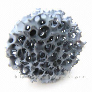
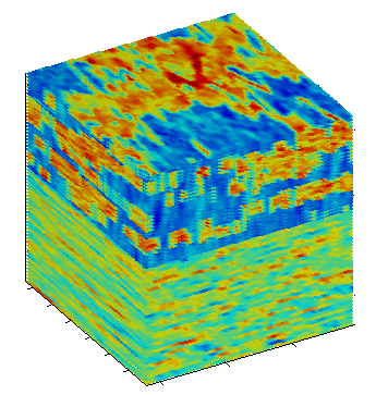
Many porous media are characterized by very low solid volume fraction and thus high porosity, e.g. fractured or vuggy reservoirs, mineral wool, and industrial foams, (cf. Figure 1 (A)). For such media the porosity could be as high as 95 – 98 %. For such highly porous media Darcy’s law often does not give good agreement with the experimental data. In order to reduce the deviations between the measurements for flows in highly porous media and the Darcy-based predictions, Brinkman in [9] introduced a new phenomenological relation between the velocity and the pressure gradient $\nabla p=-\kappa(x)\bm{u}+\mu\Delta\bm{u}$, (see, [26, page 94]). Together with conservation of mass, which in the absence of any mass sources or sinks is expressed by $\nabla\cdot\bm{u}=0$, Brinkman’s relations and proper boundary conditions form a closed mathematical model (1). An important characteristic is the contrast of the media $\bm{\kappa}$, defined as the ratio between the highest and lowest values of the permeability, $\bm{\kappa}=\max_{x\in\Omega}K(x)/\min_{x\in\Omega}K(x)$. The problems we consider in this paper involve $K(x)$ varying by orders of magnitude on small length scales.

Darcy’s and Brinkman’s equations were introduced as phenomenological macroscopic equations without direct link to underlying microscopic structure of the media. Advances in homogenization theory made it possible to rigorously derive them from Stokes’ equations for periodic media, see e.g. [1]. As concluded in [1, pp. 266–273], there are three different limits depending on the size of the periodically arranged obstacles, which respectively lead to Darcy’s, Brinkman’s, and Stokes’ equations as macroscopic, i.e., homogenized, relation. There is still ongoing discussion about the validity and the applications of Brinkman equations as a model of flows in porous media at higher values of the porosity, see, e.g. [5, 14]. Nevertheless, Brinkman’s system of equations is a convenient model of flows in highly heterogeneous porous media with random distribution of inclusions, obstacles, channels, layers and other geophysical features.

The Darcy/Brinkman model has been used also in the framework of fictitious domain methods that allows to treat in a unified way flows in porous media, [29], time dependent incompressible viscous flows, [10, 17, 27], and transient compressible viscous flows, [41]. A rigorous analysis of Brinkman’s system from the point of view of the fictitious domain method was carried out in [2, 27]. As a result, Stokes equations in a complicated domain (flow around many obstacles, an obstacle with complicated topology, or domains with void or caverns, e.g. Figure 1 (A)), are replaced by Brinkman’s equations in a simpler domain but with highly varying $\kappa(x)$. In such models the values of $\kappa(x)$ in the obstacle/void plays a role of a penalty parameter that is directly related to the contrast $\bm{\kappa}$ so that large variations in $\kappa(x)$ lead to ill-conditioning of the corresponding discrete problem.

In this paper we consider a unified approach to approximation of the Brinkman/Darcy flow equations by $H^{\text{div}}$-conforming Raviart-Thomas mixed finite elements (cf. [13] for Navier-Stokes equations and [16] for Darcy-Stokes coupling). Close to our research, discontinuous Galerkin (DG) FEM with $H^{\text{div}}$-conforming elements has also been applied to numerically solve the Brinkman system in  [28], where a priori and a posteriori error analysis in both Darcy and Brinkman limits are performed. This discretization is applied on fine meshes resolving mesoscale heterogeneities of the media. That is, we assume a homogenized microscale structure of material below grid resolution and changes of this microstructure are resolved. For example, certain media are discretized with $256^{d}$ or $512^{d}$ ($d=2,3$ is the space dimension) voxels. Discretization on such grids results in very large algebraic saddle point problems which are ill-conditioned due to both, the small mesh size and high contrast $\bm{\kappa}$.

When the jumps in the permeability are aligned with a coarse mesh, techniques based on domain decomposition, geometric multigrid or multilevel methods could lead to efficient and optimal methods for Darcy’s model, e. g. [31, 37, 38, 39]. A multigrid preconditioner for solving algebraic systems resulting from finite element approximation in $H^{\text{div}}$ was proposed by Arnold, Falk, and Winther in [3, 4]. The analysis of the preconditioner relies on the regularity of the solution. In various practical computations, it was demonstrated that this preconditioner is robust with respect to the contrast $\bm{\kappa}$ for Darcy’s model, e.g. [37, Tables 4,5] and [38, Tables 2.3 – 2.7]. However, when the jumps in the permeability are not aligned with the coarse mesh the multigrid (or multilevel) method performance deteriorates when the contrast gets larger, e.g. [31, Table 7.10]. Robust with respect to the contrast $\bm{\kappa}$ multilevel preconditioners based on additive Schur complement approximation were recently proposed and experimentally studied in [30] for the Darcy system.

The class of problems we consider in this paper is characterized by large variations of the permeability on a very fine scale (high frequency) which results in low regularity of the solution. Also, the permeability is given on a fine scale and there is no practical way to split the domain into a fixed number of subdomains where the permeability is smooth or constant. To solve such system we use a multigrid preconditioner consistent with the divergence free subspace and employing a smoother that uses patches around grid vertexes and based on the idea of Arnold, Falk, and Winther [3, 4]. As shown recently in [23, 24], this preconditioner is optimal for divergence-conforming DG approximations of Stokes’ equations. The goal of this paper is to study numerically the performance of this multigrid approach to solving the Darcy/Brinkman system for high contrast and high frequency porous media.

Preconditioning of DG FEM for Brinkman equations was considered in [15]. It was proven theoretically and confirmed experimentally that in two space dimensions the proposed preconditioner based on domain decomposition technique (or two-level method) that involves solution of some local spectral problems is optimal with respect to both, the mesh-size and the contrast. Multilevel generalization of the same idea applied to anisotropic problems was done in [42] and extended to abstract symmetric and positive definite forms in [43]. The numerical experiments in [42, 43] show that the proposed method is robust with respect to both the mesh-size and media contrast. However, the theory depends on a number of assumptions that might be difficult to verify for media of high contrast and high frequency permeability. Nevertheless, the results in [42, 43], in our opinion, present the state of the art of preconditioning of such problems.

The numerical simulation of processes in media of high frequency and high contrast represents a great challenge since it leads to ill-conditioned symmetric but indefinite system of linear equations. In our opinion, its efficient preconditioning is not fully mastered. Here we present a step in this direction for Brinkman/Darcy models. The main objectives and contributions of our paper are:

1. To discuss and present a unified solution methodology for computer simulation of flows in porous media modeled by Darcy and Brinkman equations. Using this methodology, one may set up natural experiments with highly heterogeneous media in order to compare and analyze the numerical simulations in the framework of a mathematical modeling tool.

2. To show the efficiency of the developed preconditioner for solving very large systems of linear equations arising from the finite element approximation of the Darcy and Brinkman equations and to demonstrate via various tests the robustness of the method with respect to both, the mesh step-size and the high contrast high frequency porous media.

3. To experiment with various two- and three-dimensional synthetic test problems that are used by flow in porous media community and show the capabilities of numerical simulation methodology for solving relevant applied problems.

The remainder of this paper is organized as follows: In Section 2, we provide a detailed description of the problems under consideration as well as the necessary notation. Further, we provide a description of a DG discretization of Brinkman’s equations. In Section 3 we outline the derivation of the multigrid algorithm for Brinkman’s and Darcy’s equations. In Section 4 we present numerical experiments with benchmark problems that demonstrate the capabilities and the robustness of our method. In the final Section 5 we present the main conclusions of the paper.

2. Problem Formulation and Notation

2.1. Notation of spaces

We use the standard notation for spaces of scalar and vector functions defined on a bounded domain $\Omega\subset\mathbb{R}^{d}$ ($d=2,3$) with polyhedral boundary having the outward unit normal vector $\bm{n}$. $L^{2}_{0}(\Omega)\subset L^{2}(\Omega)$ denotes the space of square integrable functions with mean value zero and $H^{1}(\Omega)^{d}$, $H^{1}_{0}(\Omega)^{d}$, and $L^{2}(\Omega)^{d}$ denote the spaces of vector-valued functions with components in $H^{1}(\Omega)$, $H^{1}_{0}(\Omega)$, and $L^{2}(\Omega)$, respectively. Furthermore, we set

$$H^{\text{div}}(\Omega) =\{\bm{v}\in L^{2}(\Omega)^{d} \;:\; \nabla\!\cdot\!\bm{v}\in L^{2}(\Omega)\}.$$

The spaces $H^{\text{div}}(\Omega)$ and $H^{1}(\Omega)^{d}$ are equipped with the following inner products

$$(\bm{u},\bm{v})_{H^{\text{div}}(\Omega)}=\displaystyle{\int_{\Omega}}(\nabla\!\cdot\!\bm{u}\,\nabla\!\cdot\!\bm{v}+\bm{u}\cdot\bm{v})~{}d\bm{x},\quad\mbox{and}\quad(\bm{u},\bm{v})_{H^{1}(\Omega)}=\displaystyle{\int_{\Omega}}(\nabla\bm{u}:\nabla\bm{v}+\bm{u}\cdot\bm{v})~{}d\bm{x},$$

and corresponding norms $\left\|\bm{v}\right\|_{H^{\text{div}}(\Omega)}^{2}=(\bm{u},\bm{v})_{H^{\text{div}}(\Omega)}\ \ \mbox{and}\ \ \left\|\bm{v}\right\|_{H^{1}(\Omega)}^{2}=(\bm{u},\bm{v})_{H^{1}(\Omega)}.$

2.2. Problem formulation

We consider the Brinkman/Darcy model for the macroscopic pressure $p$ and the fluid velocity $\bm{u}=(u_{1},\ldots,u_{d})$:

(1) $$-\mu\Delta\bm{u}+\kappa\bm{u}+\nabla p=\bm{f},\quad\nabla\!\cdot\!\bm{u}=0\quad\text{on }\partial\Omega.$$

Note that formally one gets the Darcy model by setting $\mu=0$. To this system we add proper boundary conditions. We shall consider the simplest ones

(2) $$\bm{u}=\bm{g}\quad\left(\text{or }\bm{u}\cdot\bm{n}=\bm{g}\cdot\bm{n}\text{ if }\mu=0\right)\quad\text{on }\partial\Omega.$$

We assume that the boundary data $\bm{g}\in H^{\frac{1}{2}}(\partial\Omega)^{d}$ (or $\bm{g}\cdot\bm{n}\in H^{-\frac{1}{2}}(\partial\Omega)$ for the Darcy model) and satisfy the compatibility condition

$$\int_{\partial\Omega}\bm{g}\cdot\bm{n}~{}ds=0.$$

Problem (1) has unique solutions $(\bm{u},p)$ in $H^{1}(\Omega)^{d}\times L^{2}_{0}(\Omega)$ or, if $\mu=0$, in $H^{\text{div}}(\Omega)\times L^{2}_{0}(\Omega)$. The smoothness of the solutions of these problems can be studied by the methods developed e.g. in [18]. However, due to the media character, high contrast and high frequency, this problem has limited solution regularity, which depends on the coefficients jumps and their arrangement in rather unfavorable way.

2.3. Discontinuous Galerkin (DG) Finite Element Method

For the finite element approximation of (1) we shall employ Raviart-Thomas finite elements. To this end, we partition the domain $\Omega$ into rectangular and hexahedral cells of size $h$ in two and three dimensions, respectively, and denote this partitioning by $\mathcal{T}_{h}$. Further, we shall need a notation for the set ${\mathcal{F}}^{0}_{h}$ of the internal and ${\mathcal{F}_{h}^{\partial}}$ for the boundary interfaces/edges of the finite element partition.

Now, let $\mathscr{Q}_{h}\subset L^{2}_{0}(\Omega)$ be the space of discontinuous functions that are polynomial of degree $k>0$ in each variable $x_{i}$, $i=1,\dots,d$ and $\mathscr{V}_{h}\subset H^{\text{div}}(\Omega)$ be a finite element space based on Raviart-Thomas ($RT_{k}$) elements of degree $k\geq 0$ (cf. e.g. [8, pages 120–130]). Since $\mathscr{V}_{h}\not\subseteq H^{1}(\Omega)^{d}$ the gradient of functions in $\mathscr{V}_{h}$ will be defined only in the interior of each element. Nevertheless, the theory of DG FEM developed in  [12] for $k\geq 1$ shows that the scheme is stable and has optimal approximation properties. In the special case of lowest order Raviart-Thomas elements ($RT_{0}$ or $k=0$), the gradient is not approximated consistently and the theory in [12] fails. Nevertheless, it was shown in [22], that in this case we get the MAC scheme of Harlow and Welch [19], for which an alternative theory exists, e.g. [35].

If $T_{1}$ and $T_{2}$ are two mesh cells with a common face $F$ and $\bm{v}_{1}$ and $\bm{v}_{2}$ are the traces of a function $\bm{v}\in\mathscr{V}_{h}$ on $F$ from $T_{1}$ and $T_{2}$, respectively, then we define the average and the jump by

(3) $$\{\!\!\{\bm{v}\}\!\!\}=\frac{1}{2}(\bm{v}_{1}+\bm{v}_{2})\quad\mbox{and}\quad\mbox{$\left[\left[{\bm{v}}\right]\right]$}=\bm{v}_{1}-\bm{v}_{2}\quad\mbox{for}\quad x\in F,\,\,F\in{\mathcal{F}}^{0}_{h}.$$

For the jump to be defined consistently, we assume that there is a global ordering of the finite elements so that $T_{1}$ is the element with a smaller number and $T_{2}$ is the one with higher number. It is useful to have the same notation for faces that are on the boundary $\partial\Omega$, namely, $\{\!\!\{\bm{v}\}\!\!\}=\bm{v}$ and $\mbox{$\left[\left[{\bm{v}}\right]\right]$}=\bm{v}$ on $F\subset\partial\Omega$.

Now we introduce the following notations for integrals of vector functions $\bm{u}_{h},\bm{v}\in\mathscr{V}_{h}$ over the domain $\Omega$ and over the finite element interfaces:

$$(\nabla\bm{u}_{h},\nabla\bm{v})_{\mathcal{T}_{h}}=\sum_{T\in\mathcal{T}_{h}}\int_{T}\nabla\bm{u}_{h}:\nabla\bm{v}dx,\quad\langle\mbox{$\left[\left[{\bm{u}_{h}}\right]\right]$},\mbox{$\left[\left[{\bm{v}}\right]\right]$}\rangle_{{\mathcal{F}}_{h}}=\sum_{F\in{\mathcal{F}}_{h}}\int_{F}\mbox{$\left[\left[{\bm{u}_{h}}\right]\right]$}\cdot\mbox{$\left[\left[{\bm{v}}\right]\right]$}\,ds$$

and similarly for $\langle\{\!\!\{\bm{u}_{h}\}\!\!\},\mbox{$\left[\left[{\bm{v}}\right]\right]$}\rangle_{{\mathcal{F}}_{h}}$. Further we will use also the notation

$$\bigl{<}\bm{u}_{h},\bm{v}\bigr{>}_{{\mathcal{F}}^{0}_{h}}:=\sum_{F\in{\mathcal{F}}^{0}_{h}}\int_{F}\bm{u}_{h}\cdot\bm{v}\,ds\quad\mbox{and}\quad\bigl{<}\bm{u}_{h},\bm{v}\bigr{>}_{{\mathcal{F}_{h}^{\partial}}}:=\sum_{F\in{\mathcal{F}_{h}^{\partial}}}\int_{F}\bm{u}_{h}\cdot\bm{v}\,ds=\int_{\partial\Omega}\bm{u}_{h}\cdot\bm{v}\,ds.$$

Thus, for function $\bm{u}_{h},\bm{v}\in V_{h}$ we have the following obvious relations:

$$\bigl{<}\mbox{$\left[\left[{\bm{u}_{h}}\right]\right]$},\mbox{$\left[\left[{\bm{v}}\right]\right]$}\bigr{>}_{{\mathcal{F}}_{h}}=\bigl{<}\mbox{$\left[\left[{\bm{u}_{h}}\right]\right]$},\mbox{$\left[\left[{\bm{v}}\right]\right]$}\bigr{>}_{{\mathcal{F}}^{0}_{h}}+\bigl{<}\bm{u}_{h},\bm{v}\bigr{>}_{{\mathcal{F}_{h}^{\partial}}},\quad\bigl{<}\{\!\!\{\bm{u}_{h}\}\!\!\},\mbox{$\left[\left[{\bm{v}}\right]\right]$}\bigr{>}_{{\mathcal{F}}_{h}}=\bigl{<}\{\!\!\{\bm{u}_{h}\}\!\!\},\mbox{$\left[\left[{\bm{v}}\right]\right]$}\bigr{>}_{{\mathcal{F}}^{0}_{h}}+\bigl{<}\bm{u}_{h},\bm{v}\bigr{>}_{{\mathcal{F}_{h}^{\partial}}}.$$

We use a discontinuous Galerkin (DG) finite element method to discretize problem (1). Following [13, 25], we define the interior penalty bilinear form for $\bm{u}_{h},\,\bm{v}\in\mathscr{V}_{h}$ and for $\sigma_{h}=\sigma/h$, $\sigma>0$ a sufficiently large stabilization parameter

(4) $$\begin{split}a_{h}(\bm{u}_{h},\bm{v})=&\mu(\nabla\bm{u}_{h},\nabla\bm{v})_{\mathcal{T}_{h}}+(\kappa\bm{u}_{h},\bm{v})_{\mathcal{T}_{h}}+2\mu{\sigma_{h}}\bigl{<}\mbox{$\left[\left[{\bm{u}_{h}}\right]\right]$},\mbox{$\left[\left[{\bm{v}}\right]\right]$}\bigr{>}_{{\mathcal{F}}_{h}}\\ &-\mu\bigl{<}\{\!\!\{\nabla\bm{u}_{h}\}\!\!\}\cdot\bm{n},\mbox{$\left[\left[{\bm{v}}\right]\right]$}\bigr{>}_{{\mathcal{F}}_{h}}-\mu\bigl{<}\{\!\!\{\nabla\bm{v}\}\!\!\}\cdot\bm{n},\mbox{$\left[\left[{\bm{u}_{h}}\right]\right]$}\bigr{>}_{{\mathcal{F}}_{h}},\end{split}$$

where $\{\!\!\{\nabla\bm{v}\}\!\!\}$ is the average of the $d\times d$ matrix $\nabla\bm{v}$ and $\bm{n}$ is a unit normal vector, fixed for each internal face $F\in{\mathcal{F}}^{0}_{h}$ and pointing outward $\Omega$ for a boundary face $F\subset\partial\Omega$.

The discrete weak formulation of (1) reads now: find $(\bm{u}_{h},p_{h})\in\mathscr{V}_{h}\times\mathscr{Q}_{h}$, such that

(5) $$\mathcal{A}_{h}(\bm{u}_{h},p_{h};\bm{v},q):=a_{h}(\bm{u}_{h},\bm{v})-(p_{h},\nabla\!\cdot\!\bm{v})-\bigl{(}q,\nabla\!\cdot\!\bm{u}_{h}\bigr{)}=\mathcal{F}(\bm{v},q),\quad\forall(\bm{v},q)\in\mathscr{V}_{h}\times\mathscr{Q}_{h},$$

where $\mathcal{F}(\bm{v},q)$ contains the right-hand side $\bm{f}$ and the Dirichlet boundary data $\bm{g}$:

(6) $$\mathcal{F}(\bm{v},q)=(\bm{f},\bm{v})+2\mu\sigma_{h}\bigl{<}\bm{g},\bm{v}\bigr{>}_{{\mathcal{F}_{h}^{\partial}}}-\mu\bigl{<}\nabla\bm{v}\cdot\bm{n},\bm{g}\bigr{>}_{{\mathcal{F}_{h}^{\partial}}}.$$

The discussion on the existence and uniqueness of solutions for the Brinkman system  (5), (6) can be found in  [20, 34]. We get Darcy case by taking $\mu=0$ and $\mathcal{F}(\bm{v},q)=(\bm{f},\bm{v})+\bigl{<}\bm{g}\cdot\bm{n},q\bigr{>}_{{\mathcal{F}_{h}^{\partial}}}$.

3. The multigrid method

The preconditioner is based on the geometric multigrid method that uses a hierarchy of meshes $\mathcal{T}_{j}$, $j=0,\dots,J$. The mesh $\mathcal{T}_{0}$ is the initial coarse grid partition and $\mathcal{T}_{J}\equiv\mathcal{T}_{h}$ is the finest grid, where the approximation (5)–(6) is set. The mesh hierarchy is defined recursively, such that the cells of $\mathcal{T}_{j+1}$ are obtained by splitting each cell of $\mathcal{T}_{j}$ into $2^{d}$ children by connecting the edge, face, and cell midpoints (refinement). These meshes are nested in the sense that every cell of $\mathcal{T}_{j}$ is equal to the union of its four children (eight in 3-D case). We define the mesh size $h_{j}$ as the maximum of the diameters of the cells of $\mathcal{T}_{j}$.

3.1. Nested FE spaces

Applying the finite element spaces introduced above to the meshes $\mathcal{T}_{j}$, we obtain a nested sequence of spaces

$$\begin{array}[]{rcccccl}\mathscr{V}_{0}&\subset&\mathscr{V}_{1}&\subset&\dots&\subset&\mathscr{V}_{J},\\ \mathscr{Q}_{0}&\subset&\mathscr{Q}_{1}&\subset&\dots&\subset&\mathscr{Q}_{J}.\\ \mathscr{V}_{0}\times\mathscr{Q}_{0}=:\mathscr{X}_{0}&\subset&\mathscr{X}_{1}&\subset&\dots&\subset&\mathscr{X}_{J}:=\mathscr{V}_{J}\times\mathscr{Q}_{J}.\\ \end{array}$$

The nestedness of the spaces implies that there is a sequence of natural injections $\mathcal{I}_{j}:\mathscr{X}_{j}\to\mathscr{X}_{j+1}$ of the form $\mathcal{I}_{j}(v_{j},q_{j})=(I_{j,u}v_{j},I_{j,p}q_{j})$, such that

$$I_{j,u}:\mathscr{V}_{j}\to\mathscr{V}_{j+1},\qquad I_{j,p}:\;\mathscr{Q}_{j}\to\mathscr{Q}_{j+1}.$$

From the cochain complex properties of the Raviart-Thomas spaces, we have additionally, that the divergence free subspaces $\mathscr{V}_{j}^{0}$ are nested and thus there holds $I_{j,u}:\mathscr{V}_{j}^{0}\to\mathscr{V}_{j+1}^{0}$. The $L^{2}$-projection from $\mathscr{X}_{j+1}\to\mathscr{X}_{j}$ is defined by $\mathcal{I}^{t}_{j}(v_{j},q_{j})=(I^{t}_{j,u}v_{j},I^{t}_{j,p}q_{j})$ with

(7) $$\begin{split}\bigl{(}v_{j+1}-I^{t}_{j,u}v_{j+1},w_{j}\bigr{)}&=0\quad\forall w_{j}\in\mathscr{V}_{j}\\ \bigl{(}q_{j+1}-I^{t}_{j,p}q_{j+1},r_{j}\bigr{)}&=0\quad\forall r_{j}\in\mathscr{Q}_{j}.\end{split}$$

3.2. The variable V-cycle algorithm

Due to the multilevel structure of the spaces $\mathscr{V}_{j}\times\mathscr{Q}_{j}$, $j=0,\dots,J$, on each grid level $j$ the weak formulation to find $(\bm{u}_{j},p_{j})\in\mathscr{V}_{j}\times\mathscr{Q}_{j}$ such that

(8) $$\mathcal{A}_{j}(\bm{u}_{j},p_{j};\bm{v},q)=\bigl{(}\bm{f},\bm{v}\bigr{)}\,\,\,\forall(\bm{v},q)\in\mathscr{V}_{j}\times\mathscr{Q}_{j},$$

is rewritten in an algebraic form $\bm{A}_{j}x=b_{j}$, where $x_{j}=(u_{j},p_{j})$ and $b_{j}=(f_{j},g_{j})$. Then the discretization  (5), (6) on the finest grid has the following algebraic form

$$\bm{A}_{J}x_{J}=b_{J}.$$

The system has saddle point structure with respect to the variables for velocity and pressure. We solve it by a preconditioned GMRES iteration. Due to the elliptic structure of the Brinkman operator, we choose the multilevel preconditioner $\bm{B}_{J}$ defined in the remainder of this section. We assume that the coarse mesh $\mathcal{T}_{0}$ has small number of degrees of freedom so we can afford direct solution of the system $\bm{A}_{0}x_{0}=b_{0}$.

We define the preconditioner $\bm{B}_{j}:\mathscr{X}_{j}\rightarrow\mathscr{X}_{j}$ recursively. Let $\bm{R}_{j}$ being a suitable smoother, as described below and let $m(j)$ be the number of smoothing steps on level $j$. Let $\bm{B}_{0}=\bm{A}_{0}^{-1}$. For $j=1,\ldots,J$ define the action of $\bm{B}_{j}$ on a vector $b_{j}:=(f_{j},g_{j})\in\mathscr{X}_{j}$ as follows:

1. Pre-smoothing: begin with $x_{0}=0\in\mathscr{X}_{j}$ and compute $x_{i}\in\mathscr{X}_{j}$ with $i=1,\dots,m(j)$ by

   $$x_{i}=x_{i-1}+\bm{R}_{j}\left(b_{j}-\bm{A}_{j}x_{i-1},\right).$$

2. Coarse grid correction:

   $$x_{m(j)+1}=\bm{B}_{j-1}\mathcal{I}_{j-1}^{t}\left(b_{j}-\bm{A}_{j}\,x_{m(j)}\right).$$

3. Post-smoothing: for $i=m(j)+2,\dots,2m(j)+1$ compute

   $$x_{i}=x_{i-1}+\bm{R}_{j}\left(b_{j}-\bm{A}_{j}\,x_{i-1},\right).$$

4. Assign: $\bm{B}_{j}b_{j}=x_{2m(j)+1}.$

We distinguish between the standard V-cycle with $m(j)=m(J)$ and the variable V-cycle with $m(j)=m(J)2^{J-j}$, where the number $m(J)$ of smoothing steps on the finest level is a parameter. In our numerical examples below we use the variable V-cycle with $m(J)=2$. We refer to $\bm{B}_{J}$ as the V-cycle preconditioner of $\bm{A}_{J}$, independent of the choice of $m(j)$.

3.3. Overlapping Schwarz smoothers

In this subsection, we define a class of smoothing operators $\bm{R}_{j}$ based on a subspace decomposition of the space $\mathscr{X}_{j}$. Let $\mathcal{N}_{j}$ be the set of vertices in the triangulation $\mathcal{T}_{j}$, and let $\mathcal{T}_{j,\upsilon}$ be the set of cells in $\mathcal{T}_{j}$ sharing the vertex $\upsilon$ (see Figure 2). They form an overlapping covering with $N_{j}$ patches ($N_{j}>0$), denoted by $\{\Omega_{j,\upsilon}\}_{\upsilon=1}^{N_{j}}$.

Figure 2. Part of the domain consisting of patches around four vertices (left). In the center we have a patch around the vertex 1 and on the right – a patch around the vertex 2

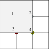
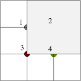
The subspace $\mathscr{X}_{j,\upsilon}=\mathscr{V}_{j,\upsilon}\times\mathscr{Q}_{j,\upsilon}$ consists of the functions in $\mathscr{X}_{j}$ with support in $\Omega_{j,\upsilon}$. Note that this implies homogeneous slip boundary conditions on $\partial\Omega_{j,\upsilon}$ for the velocity subspace $\mathscr{V}_{j,\upsilon}$ and zero mean value on $\Omega_{j,\upsilon}$ for the pressure subspace $\mathscr{Q}_{j,\upsilon}$. The Ritz projection $\mathcal{P}_{j,\upsilon}:\mathscr{X}_{j}\to\mathscr{X}_{j,\upsilon}$ is defined by the equation $\mathcal{A}_{j}\bigl{(}\mathcal{P}_{j,\upsilon}x_{j},y_{j,\upsilon}\bigr{)}=\mathcal{A}_{j}\bigl{(}x_{j},y_{j,\upsilon}\bigr{)},\quad\forall y_{j,\upsilon}\in\mathscr{X}_{j,\upsilon}.$ This equation involves solving a local saddle point problem on the patch $\Omega_{j,\upsilon}$. Note that each cell belongs to not more than four (eight in case of 3-dimentions) patches $\Omega_{j,\upsilon}$, one for each of its vertices.

Following [40] we define the symmetric multiplicative Schwarz smoother $\bm{R}_{j}$, associated with the spaces $\mathscr{X}_{j,\upsilon}$, by

(10) $$\bm{R}_{j}=(\mathcal{I}-\mathcal{E}_{j}\mathcal{E}^{\ast}_{j})\bm{A}^{-1}_{j}\quad\mbox{with}\quad\mathcal{E}_{j}=\left(\mathcal{I}-\mathcal{P}_{j,N_{j}}\right)\cdots\left(\mathcal{I}-\mathcal{P}_{j,1}\right),$$

where $\mathcal{E}^{\ast}_{j}$ is the $\bm{A}_{j}$-adjoint of $\mathcal{E}_{j}$. Note that $\bm{A}^{-1}_{j}$ is never computed, it is part only of the theoretical justification and formulation of the preconditioner, see, for more details [40].

4. Numerical Experiments

We perform numerical tests on several benchmark configurations. First, we introduce several representative permeability fields. Further, these are complemented by permeability fields from the SPE10 benchmark [11].

4.1. Setting the parameters in the computational procedure.

In all numerical experiments, we use the variable V-cycle with two smoothing steps on the finest level and the symmetric, multiplicative Schwarz smoother $\bm{R}_{j}$. The penalty parameter $\sigma_{h}$ in (4), which is denoted by $\sigma_{j}$ in the multilevel setting (8), is chosen as $\sigma_{j}=(k+1)(k+2)/h_{j}$, where $h_{j}$ is the mesh-size on level $j$. The stopping criterion in the GMRES solver is set to reduce the Euclidean norm of the initial residual by $10^{-6}$.

For setting up the discrete systems $\mathcal{A}_{j}\left(x_{j},y_{j}\right)=\mathcal{F}(y_{j}),\,\,x_{j}=(\bm{u}_{j},p_{j}),\,\,\,y_{j}=(\bm{v}_{j},q_{j})$ on each level $j$ we also need the permeability on each grid level. In our implementation we use arithmetic averaging of permeabilities. Other choices are also possible, see, e.g. [33].

4.2. Tests on some characteristic permeability fields

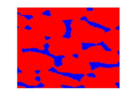
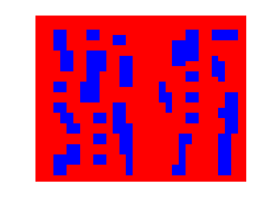
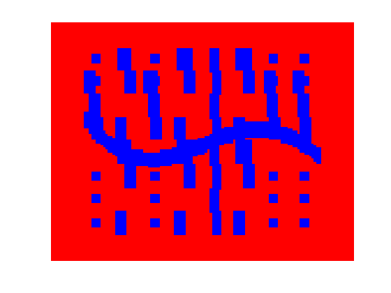
Our first numerical tests are done on a number of two dimensional permeability fields generated on a $128\times 128$ fine mesh as shown in Figure 3. Here, we have used the following convention: the red color denotes regions of media with high permeability, while the blue color corresponds to media with low permeability (in black and white – gray represents high permeability, while dark means low permeability). On Figure 3 in the red regions $\kappa(x)=1$ and in the blue regions $\kappa(x)=1/{\bm{\kappa}}$. These have been used as representative test examples by other authors, see, e.g. [32, 36].

Figure 3(A) shows the permeability of a two-dimensional cut of open foams of porous media (similar to those shown in Figure 1(A)). In this example, low permeability regions are mostly disconnected. Figures 3(B) and (C) present porous media with isolated and globally connected inclusions with low permeability. Figure 3(C) represents a media with some long connected inclusions that mimic bonded fibrous porous materials.

4.2.1. Darcy vs. Brinkman mathematical models

In order to examine the effects of numerical modeling on fluid flow in porous media, we have run tests using Darcy and Brinkman models on three different sets of permeability distribution shown in Figure 3. The flow is driven by boundary values $\bm{g}=(1,0)$ and $\bm{f}=\bm{0}$. For Brinkman’s model we use $\mu=10^{-2}$ and, obviously, $\mu=0$ for Darcy’s model. The contrast $\bm{\kappa}$ is in the range $10^{4}$ – $10^{6}$.

(a) Open foam

(b) Inclusions

(c) Connected inclusions

Figure 3. Three distributions of permeability: red regions denote high permeability, blue regions mark low permeable inclusions

(a) Open foam, Darcy

(b) Inclusions, Darcy

(c) Con. inclusions, Darcy

(d) Open foam, Brinkman

(e) Inclusions, Brinkman

(f) Con. inclusions, Brinkman

Figure 4. Velocity component $u_{1}$ for permeability distributions of Figure 3 for Darcy and Brinkman equations with contrast $\bm{\kappa}=10^{6}$: for open foam, the maximal value (red) is 3.47, minimal value (blue) is negative 0.13; for inclusions, the maximal value (red) is 3.89, minimal value (blue) negative 0.26; for connected inclusions, the maximal value (red) is 4.37, the minimal value (blue) negative 0.09.

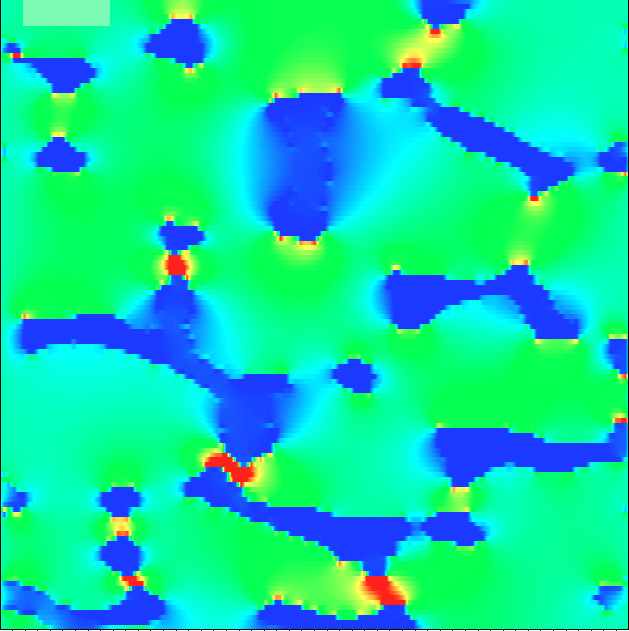
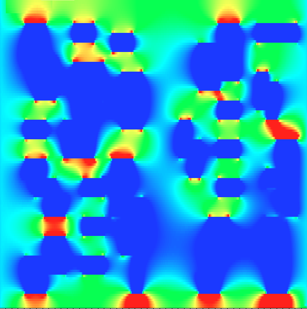
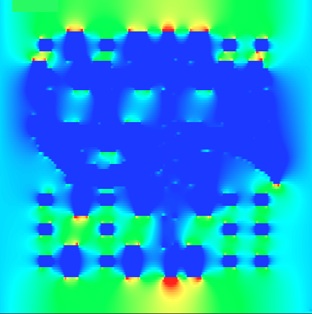
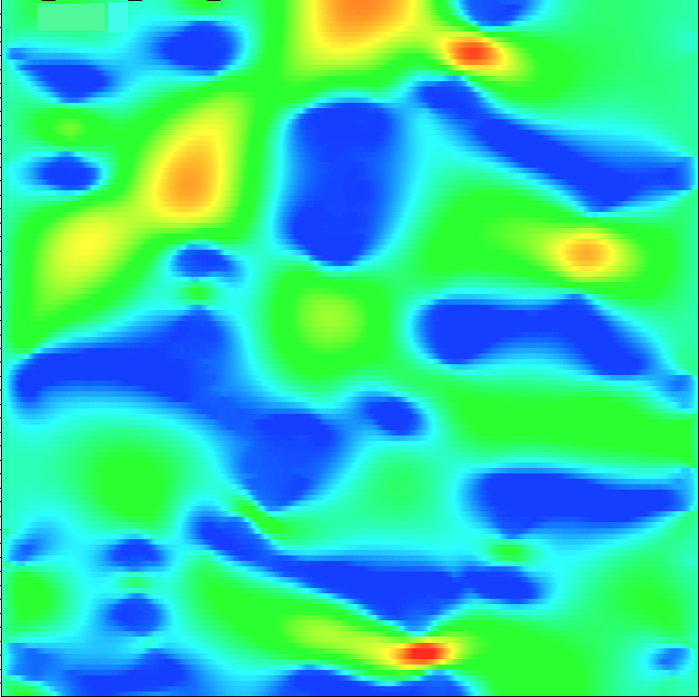
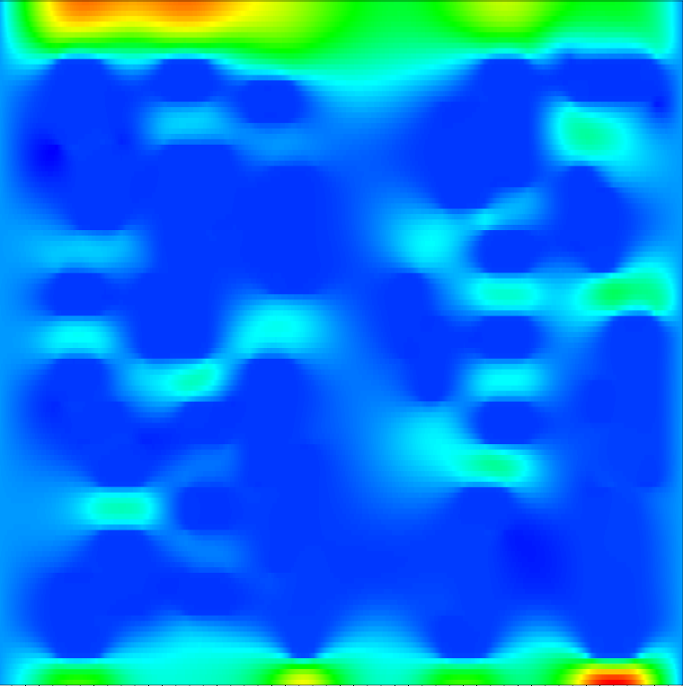
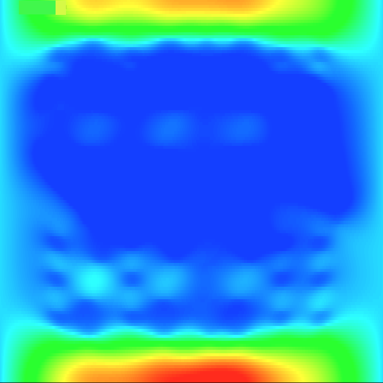
The computational results for the $u_{1}$ component of the velocity are presented in Figure 4: (A) – (C) are for Darcy and (D) – (F) – for Brinkman models. The velocity is presented in the same color scale so one can observe similarity in the patterns of the flow. One can also see different flow behaviors such as substantial variation of velocity magnitude.

One can make several immediate observations: (1) there are apparent diffusion effect in the flow governed by Brinkman model; (2) the connected inclusions, Figure 3(C), are blocking the Brinkman flow in a more profound way compared with the Darcy case; (3) the most visible differences are in the upper horizontal boundary, where no-vertical flow for both Brinkman and Darcy are imposed; in the case of Brinkman model, most of the fluid is flowing through the region adjacent to the horizontal boundaries since in the rest the flow is blocked by the inclusion that connects other long inclusions.

In addition, one visually observes a substantial difference between solutions produced by Darcy and Brinkman models while changing the permeability contrast. In order to quantify these visual difference, we computed the $H^{1}$-norm of these solutions.

More numerical experiments on these sets of data and some other permeability fields can be found in [34]. Based on these numerical experiments we observed that for Brinkman model (with permeability shown in Figure 4 (B), disconnected inclusions), the difference between the solutions obtained for $\bm{\kappa}=10^{4}$ and $\bm{\kappa}=10^{5}$ is $22\%$, while for $\bm{\kappa}=10^{5}$ and $\bm{\kappa}=10^{6}$ it is only $8\%$. Further increase of the contrast does not lead to substantial change of the solution. For Darcy and Brinkman model with the same permeability contrasts shown in Figure 4, we found that the difference between the solutions is up to $600\%$.

Based on our numerical experiments we conclude that the two numerical models produce results which are robust with respect to the parameters. The choice of the model to be used in a particular practical problem will depend on physics involved and the agreement with certain natural experiments.

4.2.2. Performance of the preconditioner on two-dimensional Darcy and Brinkman models

We also test the robustness (with respect to the contrast $\bm{\kappa}$ and the mesh-size $h$) of the preconditioner for Darcy and Brinkman models for flows in heterogeneously porous media on three sets of heterogeneous permeabilities shown in Figure 3 in two cases:

case (a):

$\kappa(x)=1$ in the blue regions (of high  permeability, channels-like formations) and $\kappa(x)=10^{-4},10^{-5},10^{-6}$ in the red regions;

case (b):

we reverse the roles of low and high permeability by taking $\kappa(x)=1$ in the red region (of low  permeability) and $\kappa(x)=10^{-4},10^{-5},10^{-6}$ in the blue regions.

	Open foam			Inclusions			Con. inclusions
	$10^{4}$	$10^{5}$	$10^{6}$	$10^{4}$	$10^{5}$	$10^{6}$	$10^{4}$	$10^{5}$	$10^{6}$
	Darcy
128	17	19	20	40	51	60	44	61	73
256	16	17	19	35	45	54	41	55	65
512	15	16	18	33	42	50	38	51	59
	Brinkman
128	18	27	36	16	22	38	16	23	36
256	16	24	32	15	20	32	14	20	31
512	15	22	31	14	19	29	13	19	29

Table 1. Number of GMRES iterations needed to reduce the residual by $10^{-6}$ for Darcy and Brinkman models for permeability shown in Figure 3

	Open foam			Inclusions			Con. inclusions
	$10^{4}$	$10^{5}$	$10^{6}$	$10^{4}$	$10^{5}$	$10^{6}$	$10^{4}$	$10^{5}$	$10^{6}$
	Darcy
128	55	67	78	76	81	88	68	74	81
256	48	61	71	68	75	82	63	69	76
512	45	58	67	64	70	78	61	64	70
	Brinkman
128	48	53	58	65	73	79	68	73	77
256	43	49	54	61	68	72	63	69	72
512	39	46	49	57	63	68	59	63	69

Table 2. Number of GMRES iterations needed to reduce the residual by $10^{-6}$ for Darcy and Brinkman models for permeability shown in Figure 3, with low and high permeability reversed

In each test of Tables 1 and 2 for a fixed permeability contrast (in a column), we observe iteration counts practically independent of the mesh size $h$. This shows that the preconditioner is uniform (possibly optimal) with respect to the mesh-size.

For a fixed fine-grid (in a row), we report the iteration count while changing the permeability in both, Darcy and Brinkman models. For a fixed contrast we observe that Brinkman model is insensitive to the distribution of the inclusions, the number of iterations is almost the same for three permeability distributions: open foams, inclusions, and connected inclusions. However, in all permeability distributions (except open foams) the iterations in both models grow with the increase of the contrast. In the case (a) by increasing the contrast 100 times the number of iterations increases by $50\%$ in Darcy model and at most $100\%$ in Brinkman model. However, the numerical experiments shown on Table 2 indicate that the iteration count is not very sensitive to the permeability distribution of case (b). These two experiments show that the preconditioner is quite sensitive to the topology of the subregions with high and low permeability.

(a) SPE10 Slice 44

(b) SPE10 Slice 49

(c) SPE10 Slice 54

(d) SPE10 Slice 74

Figure 5. Logarithmic plots of the permeability in horizontal cross sections 44, 49, 54, and 74 of three dimensional SPE10 benchmark [21], Figure 1(B)

4.3. Tests with permeability of SPE10 benchmark

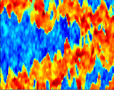
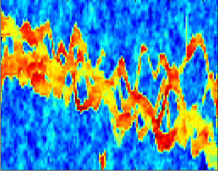
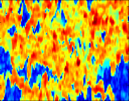
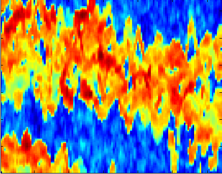
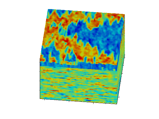
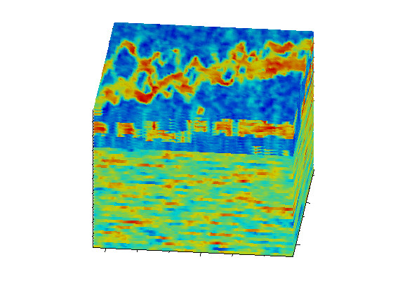
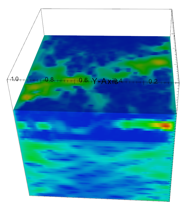
The benchmark SPE10 [11] provides permeability data on a 3-D sample represented on $60\times 220\times 85$ cells. There are 85 distinct layers within two general categories. The top 35 layers represent a prograding near shore environment with relatively low porosity and the bottom 50 layers represent a fluvial fan with channels. The data set was rescaled on a $128\times 128\times 128$-mesh, presented in Figure 1 (B). Using $RT_{0}$ elements, namely the MAC scheme on this mesh, we obtain a linear system of 15 million unknowns. In order to run additional examples, we have generated data for 2-D permeabilities, shown in Figure 5, that are horizontal slices of the SPE10 benchmark. These data sets were used to set up computational tests for 2-D Darcy and Brinkman models. The permeability is plotted in logarithmic scale, the contrast is almost $10^{8}$. One can observe diverse geological features in these slices: Slice 44, Figure 5 (A), contains two distinct highly permeable channels starting from the left that join together on the right; Slice 49 and 74, Figure 5 (B) and (D), show a single highly permeable channel (in red) with some small branches (or impermeable inclusions within it), respectively; Slice 54, Figure 5 (C), represent highly permeable region, which is almost dominated by the red and yellow regions compared to Slices 44, 49, and 74.

4.3.1. Performance of the iterative method for 2-D Darcy and Brinkman models

Here we present iteration counts of the GMRES method applied to Darcy and Brinkman models for permeability generated on horizontal slices 44, 49, 54 and 74 of the SPE10 benchmark shown on Figure 5.

	Slice 44		Slice 49		Slice 54		Slice 74
Mesh size	$RT_{0}$	$RT_{1}$	$RT_{0}$	$RT_{1}$	$RT_{0}$	$RT_{1}$	$RT_{0}$	$RT_{1}$
1/128	37 (36)	42 (41)	39 (36)	46 (42)	33 (32)	37 (35)	38 (36)	44 (43)
1/256	31 (31)	37 (37)	34 (32)	41 (38)	28 (28)	31 (30)	32 (31)	39 (38)
1/512	27 (28)	33 (33)	31 (29)	37 (34)	24 (24)	27 (27)	27 (29)	35 (34)

Table 3. Iteration count for Darcy and Brinkman (in parentheses) models with data of SPE10 benchmark (see Figure 5) with RT₀ and RT₁ finite elements

In Table 3, we present the number of iterations for Darcy and Brinkman models using $RT_{0}$ and $RT_{1}$ finite elements. For a given permeability distribution in a column, we give the number of GMRES iterations for mesh step-size varying from $1/128$ to $1/512$ and for the permeability presented on Figure  5. Clearly, the method is robust with respect to mesh-size. Moreover, analyzing the results in Table 3 we see a reduction in the number of iterations for finer meshes. A similar observation can be made for the results of Table 1 as well. A possible reason for such decrease is that the preconditioner becomes better (as we refine the mesh) due to the upscaling properties of the method, since the data is given on fixed mesh $128\times 128$).

We compared the iteration counts of our method with the recently proposed in [30, formula 4.3] block preconditioner of the Darcy system. In that paper the block corresponding to the weighted $H^{\text{div}}$-norm (namely $(\kappa\bm{u},\bm{u})+(\nabla\cdot\bm{u},\nabla\cdot\bm{u})$) is handled by special multilevel method using additive Schur complement approximation. We compare the performance of these two methods on the permeability field generated by slice 44 of SPE10 (see, Figure 5). The total number of iterations in the minimal residual method in [30] is slightly less than the iterations shown on Table 3. However, within each iteration the method, to invert the block corresponding to the weighted $H^{\text{div}}$-norm, the method in [30, Tables 12 and 13] uses in average 6 inner multilevel iterations. Our smoother is more expensive than the smoother in [30], but the total number of MG steps is much smaller. In summary, these two methods show similar performance and robustness with respect to both step size and contrast. We note that the numerical tests show that our method performs efficiently on meshes with $2048\times 2048$ (for RT₀) or $512\times 512$ (for RT₁) for both Darcy and Brinkman models.

4.3.2. Comparison of the solution of Darcy and Brinkman models

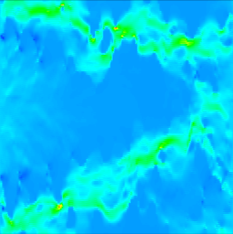
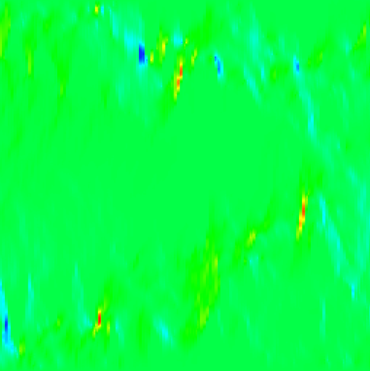
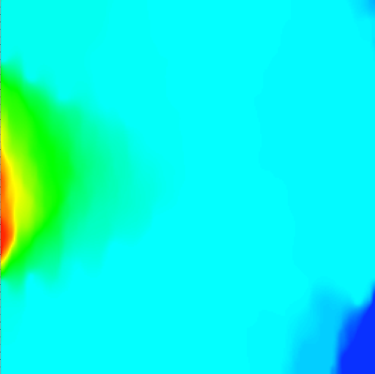
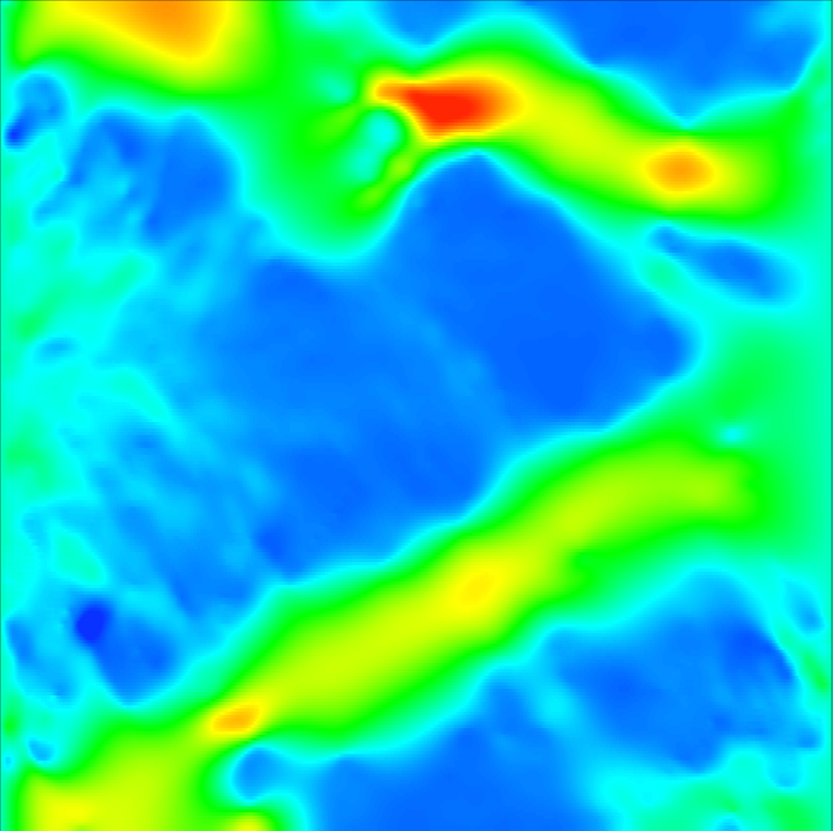
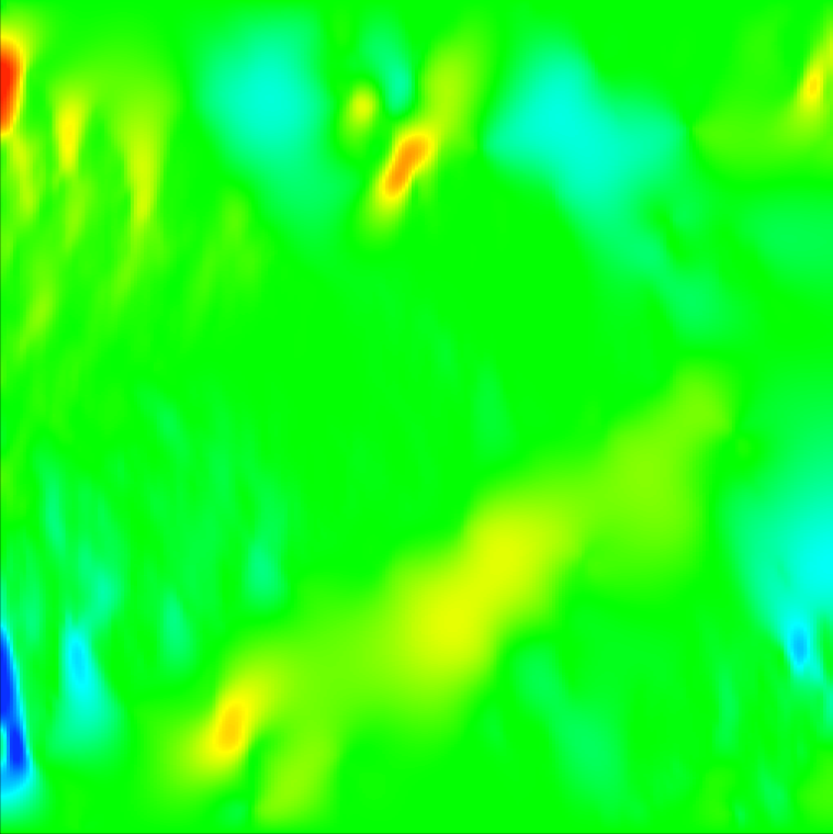
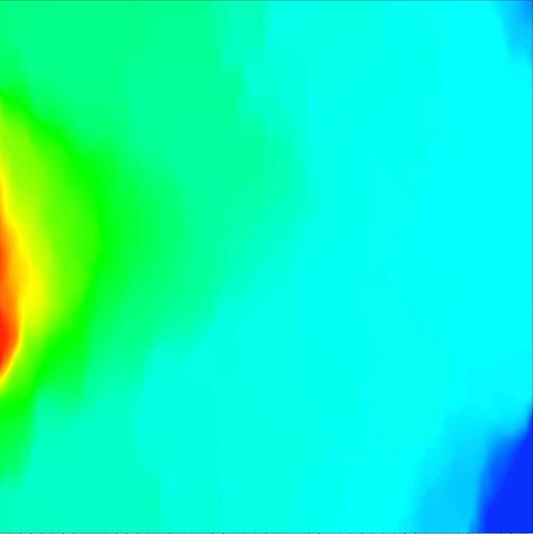
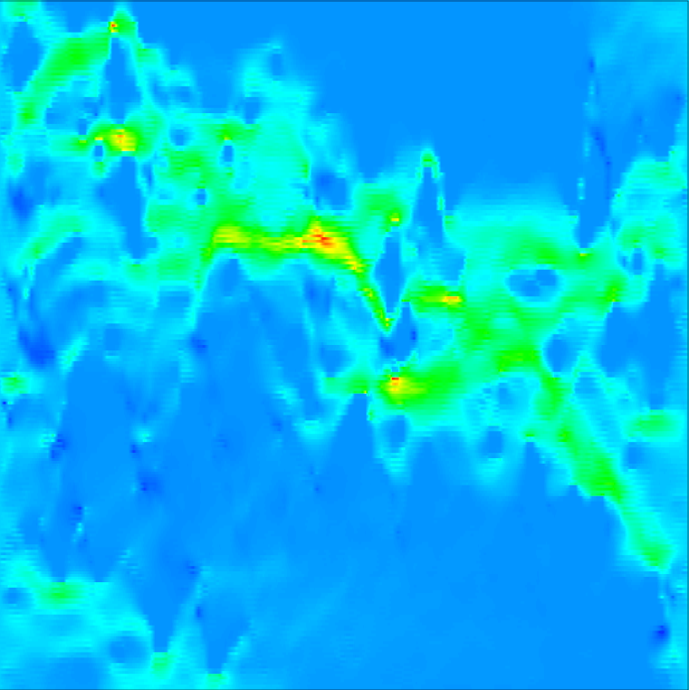
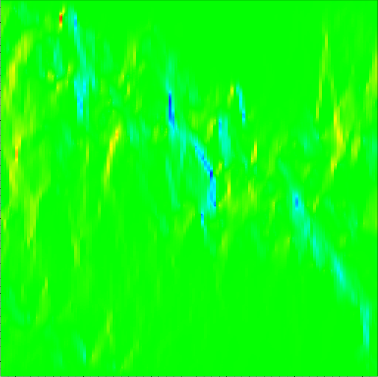
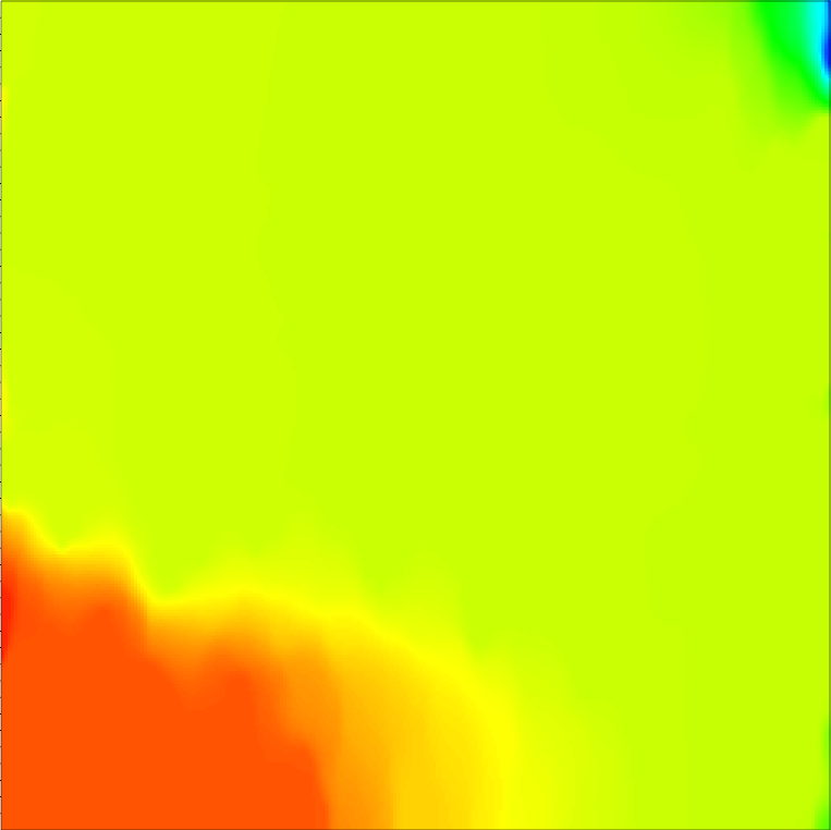
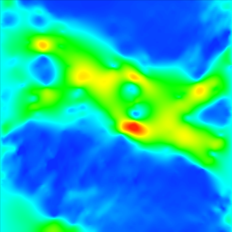
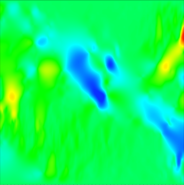
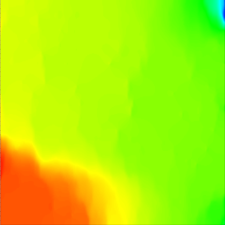
Next, we present solutions produced by the two different models for the permeability in Figures 6 and 7, respectively. Since the solutions are of low regularity we have set all experiments for $RT_{0}$ finite elements. The solutions of Darcy and Brinkman models are plotted in the same scale so we can make a visual comparison. One can observe that the pressure obtained from Darcy and Brinkman models in both slices, 44 and 49, do not differ significantly. The most substantial differences are in the velocity. One observes from this pictures that, as expected, the Brinkman model is more diffusive.

(a) Darcy: $u_{1}$

(b) Darcy: $u_{2}$

(c) Darcy: $p$

(d) Brinkman: $u_{1}$

(e) Brinkman: $u_{2}$

(f) Brinkman: $p$

Figure 6. Solution for permeability data of slice 44 in the same color scale

(a) Darcy: $u_{1}$

(b) Darcy: $u_{2}$

(c) Darcy: $p$

(d) Brinkman: $u_{1}$

(e) Brinkman: $u_{2}$

(f) Brinkman: $p$

Figure 7. Solution for permeability data of slice 74

4.3.3. Computations with 3D SPE10 benchmark

We now present and discuss briefly numerical results for the three dimensional SPE10 benchmark, see, Figure 1 (B). We set $\mu=10^{-2}$ and use Dirichlet boundary condition ${\bm{g}}=(1,0,0)$ and homogeneous right hand side, ${\bm{f}}=\bm{0}$.

In Table 4, we show the number of multigrid iterations for two different sets of boundary values and with three different stopping criteria. One can observe that the method is quite robust with respect to different stopping criteria and boundary values.

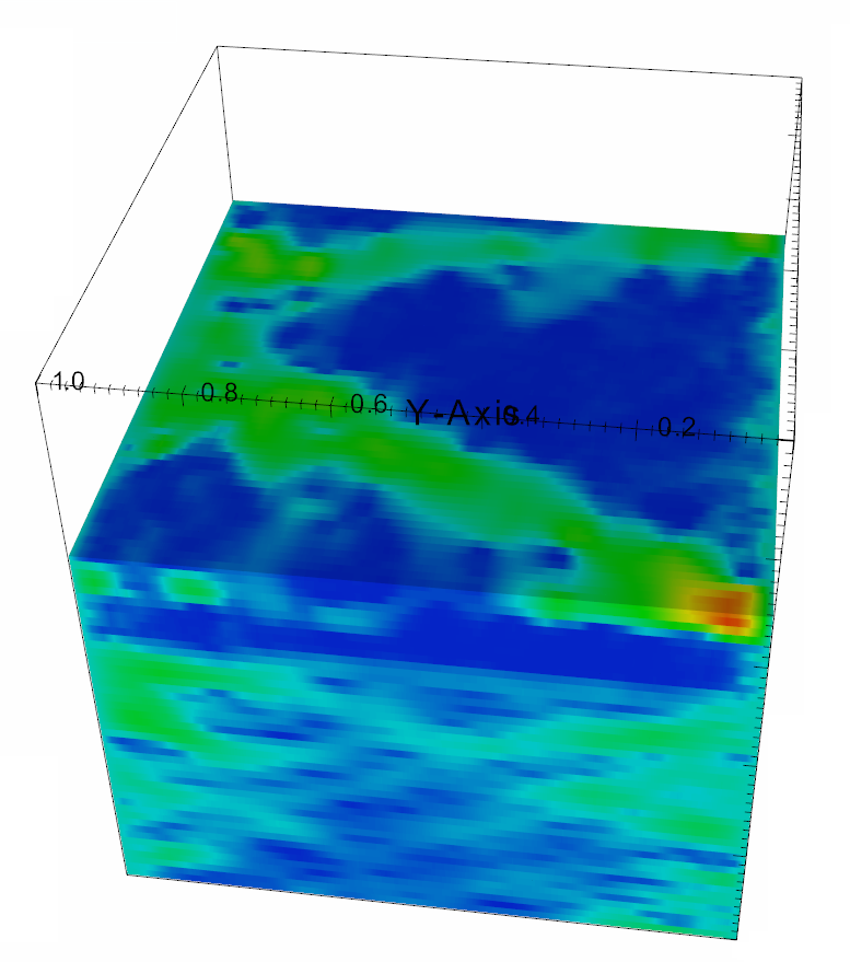
Finally, in Figure 8 we show the $u_{1}$-component of the solution in the horizontal planes corresponding to slices 44 and 49 obtained from 3-D Brinkman model solved with SPE10 benchmark permeability.

	Residual $10^{-6}$		Residual $10^{-8}$		Residual $10^{-10}$
Mesh size	$BC1$	$BC2$	$BC1$	$BC2$	$BC1$	$BC2$
1/64	40	41	55	56	81	82
1/128	31	31	46	46	73	73

Table 4. Iteration count for the 3-D Brinkman model for SPE10 with boundary data – BC1: ${\bm{g}}=(1,0,0)$ and BC2: ${\bm{g}}=(0,1,0)$

(a) Slice 44: $\kappa(x)$

(b) Slice 44: $u_{1}$

(c) Slice 49: $\kappa(x)$

(d) Slice 49: $u_{1}$

Figure 8. Brinkman - SPE10 with boundary data ${\bm{g}}=(1,0,0)$

5. Conclusions

We studied the $H^{\text{div}}$-conforming discontinuous Galerkin discretization for Darcy and Brinkman equations and presented a geometric multigrid method with a patch-based domain decomposition smoother for the corresponding algebraic system. Our numerical results show uniform contraction independent of the mesh size. In addition, we experimentally verify the robustness and efficiency of our method with respect to Darcy and Brinkman problems on two and three dimensional high contrast and high frequency distributions of the permeability. Nevertheless, iteration counts go up into the 80s when we increase the contrast to $10^{8}$. We point out though, that the geometric multigrid method with patch-based smoother is highly parallelizable. We plan to study further some algorithmic improvements like better choice of the coarse problem and parameter dependent projections.

Acknowledgments

All computations were performed using the open source finite element library deal.II [6, 7].

References

- [1] G. Allaire. Homogenization of the Navier-Stokes equations in open sets perforated with tiny holes. I: Abstract framework, a volume distribution of holes. Arch. Ration. Mech. Anal., 113(3):209–259, 1991.
- [2] P. Angot. Analysis of singular perturbations on the Brinkman problem for fictitious domain models of viscous flows. Math. Methods Appl. Sci., 22(16):1395–1412, 1999.
- [3] D. Arnold, R. Falk, and R. Winther. Preconditioning in H(div) and applications. Mathematics of Computation, 66:957–984, 1997.
- [4] D. Arnold, R. Falk, and R. Winther. Multigrid in H(div) and H(curl). Numer. Math., 85(2):197–217, 2000.
- [5] J.-L. Auriault. On the domain of validity of Brinkman s equation. Transport in Porous Media, 79(2):215–223, 2009.
- [6] W. Bangerth, R. Hartmann, and G. Kanschat. deal.II — a General Purpose Object Oriented Finite Element Library. ACM Trans. Math. Softw., 33(4), 2007.
- [7] W. Bangerth, T. Heister, L. Heltai, G. Kanschat, M. Kronbichler, M. Maier, and B. Turcksin. The deal.II library, version 8.3. Arch. Numer. Software, 2016. to appear.
- [8] F. Brezzi and M. Fortin. Mixed and Hybrid Finite Element Methods, volume 15 of Springer Series in Computational Mathematics. Springer, 1st edition, 1991.
- [9] H. Brinkman. A calculation of the viscouse force exerted by a flowing fluid on a dense swarm of particles. Appl. Sci. Res., A1:27–34, 1947.
- [10] A. Bugrov and S. Smagulov. The fictitious regions method in boundary value problems for Navier-Stokes equations. Mathematical Models of Fluid Flows (Russian), pp. 79 – 90, 1978.
- [11] M. Christie and M. Blunt. Tenth SPE comparative solution project: A comparison of upscaling techniques. SPE Reservoir Evaluation & Engineering, 4(04):308–317, 2001.
- [12] B. Cockburn, G. Kanschat, and D. Schötzau. A locally conservative LDG method for the incompressible Navier-Stokes equations. Mathematics of Computation, 74(251):1067–1095, 2005.
- [13] B. Cockburn, G. Kanschat, and D. Schötzau. A note on discontinuous Galerkin divergence-free solutions of the Navier–Stokes equations. Journal of Scientific Computing, 31(1-2):61–73, 2007.
- [14] L. Durlofsky and J. F. Brady. Analysis of the Brinkman equation as a model for flow in porous media. Physics of Fluids, 30(11):3329–3341, 1987.
- [15] Y. Efendiev, J. Galvis, R. Lazarov, and J. Willems. Robust domain decomposition preconditioners for abstract symmetric positive definite bilinear forms. ESAIM: Mathematical Modelling and Numerical Analysis, 46(05):1175–1199, 2012.
- [16] V. Girault, G. Kanschat, and B. Rivi’ere. Error analysis for a monolithic discretization of coupled Darcy and Stokes problems. J. Numer. Math., 22(2):109–142, 2014.
- [17] R. Glowinski, T.-W. Pan, and J. Périaux. A fictitious domain method for external incompressible viscous flow modeled by Navier-Stokes equations. Comp. Meth. Appl. Mech. Engng., 112:133 – 148, 1994.
- [18] P. Grisvard. Boundary Value Problems in Non-Smooth Domains. Pitman, London, 1985.
- [19] F. H. Harlow and J. E. Welch. Numerical calculation of time-dependent viscous incompressible flow of fluid with free surface. Phys. Fluids, 8(12):2182–2189, 1965.
- [20] O. Iliev, R. Lazarov, and J. Willems. Variational multiscale finite element method for flows in highly porous media. Multiscale Modeling & Simulation, 9(4):1350–1372, 2011.
- [21] S. P. E. International. SPE10 comparative solution project: general information and description of model 2, 2000. http://www.spe.org/web/csp/#datasets.
- [22] G. Kanschat. Divergence-free discontinuous Galerkin schemes for the Stokes equations and the MAC scheme. International journal for numerical methods in fluids, 56(7):941–950, 2008.
- [23] G. Kanschat and Y. Mao. Multigrid methods for H(div)-conforming discontinuous Galerkin for the Stokes. Journal of Numerical Mathematics, 23(1):51–66, 2015.
- [24] G. Kanschat and Y. Mao. Multiplicative overlapping Schwarz smoothers for H(div)-conforming discontinuous Galerkin for the Stokes problem. Domain Decomposition Methods in Science and Engineering XXII, Lecture Notes in Computational Science and Engineering, 104:285–292, 2016.
- [25] G. Kanschat and B. Rivière. A strongly conservative finite element method for the coupling of Stokes and Darcy flow. Journal of Computational Physics, 229(17):5933–5943, 2010.
- [26] M. Kaviany. Principles of Heat Transfer in Porous Media. Springer-Verlag, New York, 1991.
- [27] K. Khadra, P. Angot, S. Parneix, and J.-P. Caltagirone. Fictitious domain approach for numerical modelling of Navier-Stokes equations. International Journal for Numerical Methods in Fluids, 34:651–684, 2000.
- [28] J. Könnö and R. Stenberg. H (div)-conforming finite elements for the Brinkman problem. Mathematical Models and Methods in Applied Sciences, 21(11):2227–2248, 2011.
- [29] A. N. Konovalov. The fictitious regions method in problems of mathematical physics. Computing methods in applied sciences and enginering, Proc. 4th int. Symp., Versailles 1979, pp. 29–40, 1980.
- [30] J. Kraus, R. Lazarov, M. Lymbery, S. Margenov, and L. Zikatanov. Preconditioning heterogeneous H(div) problems by additive Schur complement approximation and applications. accepted in SISC, 2015. (early version posted as arXiv:1406.4455).
- [31] J. Kraus and S. Margenov. Robust Algebraic Multilevel Methods and Algorithms. De Gruyter Incorporated, Walter, Berlin-New York, 2009.
- [32] L.-P. Lefebvre, J. Banhart, and D. Dunand. Porous metals and metallic foams: current status and recent developments. Advanced Engineering Materials, 10(9):775–787, 2008.
- [33] M. S. Maier. Duality-based adaptivity of model and discretization in multiscale finite-element methods. PhD thesis, Heidelberg University, 2015.
- [34] Y. Mao. Geometric Multigrid methods for flow problems in Highly Heterogeneous porous media. PhD thesis, Texas A&M University, College Station, 2014.
- [35] R. A. Nicolaides. Analysis and convergence of the MAC scheme. I. the linear problem. SIAM Journal on Numerical Analysis, 29(6):1579–1591, 1992.
- [36] P. Popov, L. Bi, Y. Efendiev, R. E. Ewing, G. Qin, J. Li, Y. Ren, et al. Multi-physics and multi-scale methods for modeling fluid flow through naturally-fractured vuggy carbonate reservoirs. In SPE Middle East Oil and Gas Show and Conference. Society of Petroleum Engineers, 2007.
- [37] C. Powell. Parameter-free H(div) preconditioning for a mixed finite element formulation of diffusion problems. IMA Journal of Numerical Analysis, 25(4):783–796, 2005.
- [38] C. Powell and D. Silvester. Optimal preconditioning for Raviart–Thomas mixed formulation of second-order elliptic problems. SIAM Journal on Matrix Analysis and Applications, 25(3):718–738, 2003.
- [39] N. Spillane, V. Dolean, P. Hauret, F. Nataf, C. Pechstein, and R. Scheichl. Abstract robust coarse spaces for systems of pdes via generalized eigenproblems in the overlaps. Numerische Mathematik, 126(4):741–770, 2014.
- [40] A. Toselli and O. Widlund. Domain decomposition methods—algorithms and theory, volume 34 of Springer Series in Computational Mathematics. Springer-Verlag, Berlin, 2005.
- [41] P. N. Vabishchevich. The method of fictitious domains in problems of mathematical physics. Moscow State University Publishing House (Russian), 158 pages, Moscow, 1991.
- [42] J. Willems. Robust multilevel solvers for high-contrast anisotropic multiscale problems. Journal of Computational and Applied Mathematics, 251(1):47–60, 2013.
- [43] J. Willems. Robust multilevel methods for general symmetric positive definite operators. SIAM J. Numerical Analysis, 52(1):103–124, 2014.