Algebraic equation and quadratic differential related to generalized Bessel polynomials with varying parameters.

Abstract

The limiting set of zeros of generalized Bessel polynomials $B_{n}^{(\alpha)}$ with varying parameters depending on the degree $n$ cluster in a curve on the complex plane, which is a finite critical trajectory of a quadratic differential in the form $\lambda^{2}\frac{\left(z-a\right)\left(z-b\right)}{z^{4}}dz^{2}.$ The motivation of this paper is the description of the critical graphs of these quadratic differentials. In particular, we give a necessary and sufficient condition on the existence of short trajectories.

2010 Mathematics subject classification: 30C15, 31A35, 34E05.

Keywords and phrases: Quadratic differentials, trajectories and orthogonal trajectories, Cauchy transform, generalised Bessel and Laguerre polynomials.

1 Introduction
 

Quadratic differentials appear in many areas of mathematics and mathematical physics such as orthogonal polynomials, Teichműller spaces, moduli spaces of algebraic curves, univalent functions, asymptotic theory of linear ordinary differential equations etc…

One of the most common problems in the study of a given quadratic differential on the Riemann sphere $\overline{\mathbb{C}}$, is the description of its critical graph, and more precisely, the investigation of the existence or not of its short trajectories.

In this paper, we study on the Riemann sphere $\overline{\mathbb{C}}$ the quadratic differential

$$\varpi\left(\lambda,a,b,z\right)=\lambda^{2}\frac{\left(z-a\right)\left(z-b\right)}{z^{4}}dz^{2},$$ (1)

where $a,b,$ and $\lambda$ are three non vanishing complex numbers with $a\neq b.$ In section 2, Proposition 2 gives a necessary and sufficient condition on the existence of finite critical trajectories of $\varpi\left(\lambda,a,b,z\right).$

Quadratic differentials (1) appear in the investigation of the existence of a compactly supported positive measure $\mu$ (in the literature, such a measure $\mu$ is called positive mother-body measure) whose Cauchy transform $\mathcal{C}_{\mu}\left(z\right)$ satisfies (in some non-empty subset of $\mathbb{C}$ ) the following algebraic equation

$$z^{2}\mathcal{C}^{2}\left(z\right)-\left(pz+q\right)\mathcal{C}\left(z\right)+r=0,$$ (2)

where $p,$ $q$ and $r$ are three non vanishing complex numbers. Proposition 7 below answers this question.

In section 3, we make the connection with generalized Bessel polynomials $B_{n}^{\left(\alpha\right)}$ when the parameters determining these polynomials are complex and depend linearly on the degree.

2 Critical graph of $\varpi\left(\lambda,a,b,z\right)$

We first present a little background on the theory of quadratic differentials. For more details, we refer the reader to [4],[5],[12],[14].

Definition 1

A rational quadratic differential on the Riemann sphere $\overline{\mathbb{C}}$ is a form $\varpi=\varphi(z)dz^{2}$, where $\varphi$ is a rational function of a local coordinate $z$. If $z=z(\zeta)$ is a conformal change of variables then

$$\widetilde{\varphi}(\zeta)d\zeta^{2}=\varphi(z(\zeta))(dz/d\zeta)^{2}d\zeta^{2}$$

represents $\varpi$ in the local parameter $\zeta$.

The critical points of $\varpi\left(\lambda,a,b,z\right)$ are its zeros and poles; a critical point is finite if it is a zero or a simple pole, otherwise, it is infinite. All other points of $\overline{\mathbb{C}}$ are called regular points.

We start by observing that $\varpi\left(\lambda,a,b,z\right)$ has two simple zeros, $a$ and $b$, and, the origin is a pole of order $4$. Another pole is located at infinity and is of order 2. In fact, with the parametrization $u=1/z$, we get

$$\ \varpi\left(\lambda,a,b,z\right)=\left(-\frac{\lambda}{u^{2}}+\mathcal{O}(u^{-1})\right)du^{2},\quad u\rightarrow 0.$$

The horizontal trajectories (or just trajectories) are the zero loci of the equation

$$\mathcal{\Im}\int^{z}\lambda\frac{\sqrt{\left(t-a\right)\left(t-b\right)}}{t^{2}}\,dt=\text{\emph{const}},$$ (3)

or equivalently

$$\lambda^{2}\frac{\left(z-a\right)\left(z-b\right)}{z^{4}}dz^{2}>0.$$

The vertical (or, orthogonal) trajectories are obtained by replacing $\Im$ by $\Re$ in the equation above. The horizontal and vertical trajectories of $\varpi\left(\lambda,a,b,z\right)$ produce two pairwise orthogonal foliations of the Riemann sphere $\overline{\mathbb{C}}$.

A trajectory passing through a critical point is called critical trajectory. If it starts and ends at a finite critical points it is called finite critical trajectory or short trajectory. If it starts at a finite critical point but tends either to the origin or to infinity, we call it an infinite critical trajectory. The set of finite and infinite critical trajectories of $\varpi\left(\lambda,a,b,z\right)$ together with their limit points (infinite critical points of $\varpi\left(\lambda,a,b,z\right)$) is called the critical graph of $\varpi\left(\lambda,a,b,z\right)$.

From each zero, $a$ and $b,$ there emanate $3$ critical trajectories under equal angles $2\pi/3$. The trajectories near $\infty$ have the radial, the circle or the log-spiral forms, respectively if $\lambda\in\mathbb{R}$, $\lambda^{2}<0$, or $\lambda^{2}\notin\mathbb{R}$.

Since the origin is a pole of order $4$, there are 2 opposite asymptotic directions (called critical asymptotics) that can take any trajectory diverging to $z=0$. See Figure 1.

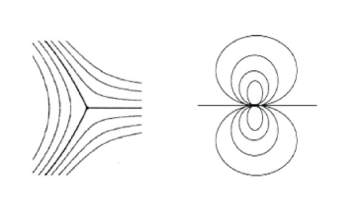
Figure 1: Local trajectories near a simple zero (left) and 4th order pole (right)

An obvious necessary condition on the existence of a short trajectory joining $a$ and $b$ is that

$$\mathcal{\Im}\int_{a}^{b}\lambda\frac{\sqrt{\left(t-a\right)\left(t-b\right)}}{t^{2}}\,dt=0,$$

where the path of integration is in $\mathbb{C}\setminus\left\{0\right\}$. Moreover, as we will see, this condition is sufficient.

The main result of this section is the following :

Proposition 2

There exists a finite critical trajectory of the quadratic differential $\varpi\left(\lambda,a,b,z\right)$ if and only if $\Re\left(\lambda\frac{\left(\sqrt{a}+\sqrt{b}\right)^{2}}{\sqrt{ab}}\right)=0$ with some choice of the square roots.

Below, given an oriented Jordan curve $\gamma$ joining $a$ and $b$ in $\mathbb{C}^{\ast}$, for $t\in\gamma$, we denote by $\left(\sqrt{\left(t-a\right)\left(t-b\right)}\right)_{+}$ and $\left(\sqrt{\left(t-a\right)\left(t-b\right)}\right)_{-}$ the limits from the $+$-side and $-$-side respectively. (As usual, the $+$-side of an oriented curve lies to the left, and the $-$-side lies to the right, if one traverses $\gamma$ according to its orientation.)

Lemma 3

For any curve $\gamma$ joining $a$ and $b$ and not passing through $0,$ we have:

$$\int_{\gamma}\dfrac{\left(\sqrt{\left(z-a\right)\left(z-b\right)}\right)_{+}}{z^{2}}dz=\pm\frac{i\pi}{2}\frac{\left(\sqrt{a}\pm\sqrt{b}\right)^{2}}{\sqrt{ab}},$$

the signs $\pm$ depend on the homotopy class of $\gamma$ in $\mathbb{C}^{\ast},$ and the branch of the square root $\sqrt{\left(z-a\right)\left(z-b\right)}$ defined in $\mathbb{C}\setminus\gamma$ is chosen so that $\sqrt{\left(z-a\right)\left(z-b\right)}\sim z,z\rightarrow\infty.$

Proof. With the above choices, consider

$$I=\int_{\gamma}\frac{\left(\sqrt{\left(z-a\right)\left(z-b\right)}\right)_{+}}{z^{2}}dz.$$

Since

$$\left(\sqrt{\left(t-a\right)\left(t-b\right)}\right)_{+}=-\left(\sqrt{\left(t-a\right)\left(t-b\right)}\right)_{-},t\in\gamma,$$

we have

$$2I =\int_{\gamma}\left[\frac{\left(\sqrt{\left(t-a\right)\left(t-b\right)}\right)_{+}}{t^{2}}-\dfrac{\left(\sqrt{\left(t-a\right)\left(t-b\right)}\right)_{-}}{t^{2}}\right]dt$$

$$=\oint_{\Gamma}\dfrac{\sqrt{\left(z-a\right)\left(z-b\right)}}{z^{2}}dz,$$

where $\Gamma$ is a closed contour encircling the curve $\gamma$ once in the clockwise direction and not encircling $z=0.$ After a contour deformation we pick up residues at $z=0$ and at $z=\infty.$ From the expressions

$$\frac{\sqrt{\left(z-a\right)\left(z-b\right)}}{z^{2}} =\allowbreak\frac{\sqrt{ab}}{z^{2}}-\frac{\sqrt{ab}\left(a+b\right)}{2ab}\frac{1}{z}+\mathcal{O}\left(1\right),z\rightarrow 0;$$

$$\frac{\sqrt{\left(z-a\right)\left(z-b\right)}}{z^{2}} =\frac{1}{z}+\mathcal{O}\left(z^{-2}\right),z\rightarrow\infty,$$

we get, for any choice of the square roots

$$I =\frac{1}{2}\oint_{\gamma}\frac{\sqrt{\left(z-a\right)\left(z-b\right)}}{z^{2}}dz=\pm i\pi\left(\underset{0}{res}+\underset{\infty}{res}\right)\left(\frac{\sqrt{\left(z-a\right)\left(z-b\right)}}{z^{2}}\right)$$

$$=\pm i\pi\left(\frac{\sqrt{ab}\left(a+b\right)-2ab}{2ab}\right)=\pm i\frac{\pi}{2}\frac{\left(\sqrt{a}\pm\sqrt{b}\right)^{2}}{\sqrt{ab}}.$$

We just proved the necessary condition of Proposition 2.   

Definition 4

A domain in $\mathbb{C}$ bounded only by segments of horizontal and/or vertical trajectories of $\varpi$ (and their endpoints) is called $\varpi$-polygon.

We can use the Teichmüller lemma (see [4, Theorem 14.1]) to clarify some facts about the global structure of the trajectories.

Lemma 5 (Teichműller)

Let $\Omega$ be a $\varpi$-polygon, and let $z_{j}$ be the singular points of $\varpi$ on the boundary $\partial\Omega$ of $\Omega,$ with multiplicities $n_{j},$ and let $\theta_{j}$ be the corresponding interior angles with vertices at $z_{j},$ respectively. Then

$$\sum\left(1-\theta_{j}\dfrac{n_{j}+2}{2\pi}\right)=2+\sum n_{i},$$

where $n_{i}$ are the multiplicities of the singular points inside $\Omega.$

Let us keep the notations of Lemma 5 and assume that $\Re\left(\lambda\right)\neq 0.$ Suppose that $\gamma_{1}$ and $\gamma_{2}$ are two trajectories emanating from $a$, spacing with angle $\theta_{a}\in\left\{\frac{2\pi}{3},\frac{4\pi}{3}\right\},$ and diverging simultaneously to the same pole $c\in$ $\left\{\infty,0\right\},$ then, they will form an $\varpi$-polygon $\Omega$ with vertices $a$ and $c.$

• If $c=\infty,$ then there is always an orthogonal trajectory intersecting $\gamma_{1}$ and $\gamma_{2}$ at the right angles; to each of these two corners, formed in this way, it corresponds the value of $\beta_{j}=\frac{1}{2}$, so their sum is $1$. Making the intersection points approach $c=\infty,$ we see that in the limit we can consider $\beta_{c}=1$ for $z_{c}=\infty$. Then

  $$\sum n_{i}=-1+\left(1-\dfrac{3\theta_{a}}{2\pi}\right)\in\left\{-2,-1\right\},$$

  which cannot hold.

• If $c=0,$ let $\theta_{0}\in\left\{0,\pi,2\pi\right\}$ be the interior angle of the $\varpi$-polygon $\Omega$ between $\gamma_{1}$ and $\gamma_{2}$ at $c=0$.

  • If $\theta_{0}=0,$ then

    $$\sum n_{i}=-\dfrac{3\theta}{2\pi}\in\left\{-2,-1\right\}.$$

    Which cannot hold.

  • If $\theta_{0}=\pi,$ then

    $$\sum n_{i}=1-\dfrac{3\theta}{2\pi}\in\left\{0,-1\right\}.$$

    Thus, $\theta=\frac{2\pi}{3}$ and $\Omega$ does not contain inside itself any critical point; see Figure 3.

  • If $\theta_{0}=2\pi,$ then

    $$\sum n_{i}=2-\dfrac{3\theta}{2\pi}\in\left\{0,1\right\}.$$

    Thus, if $\theta=\frac{2\pi}{3},$ then $\Omega$ contains inside itself the other zero $b$ and the 3 trajectories emanating from it; if $\theta=\frac{4\pi}{3},$ then $\Omega$ does not contain inside itself any critical point; see Figure 3.

    

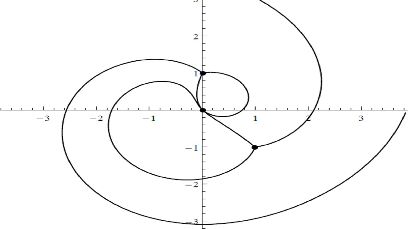
    Figure 2: $c=0$ and $\theta_{0}=\pi.$ Here $\lambda^{2}=-2-i,a=1-i,b=i$.

    

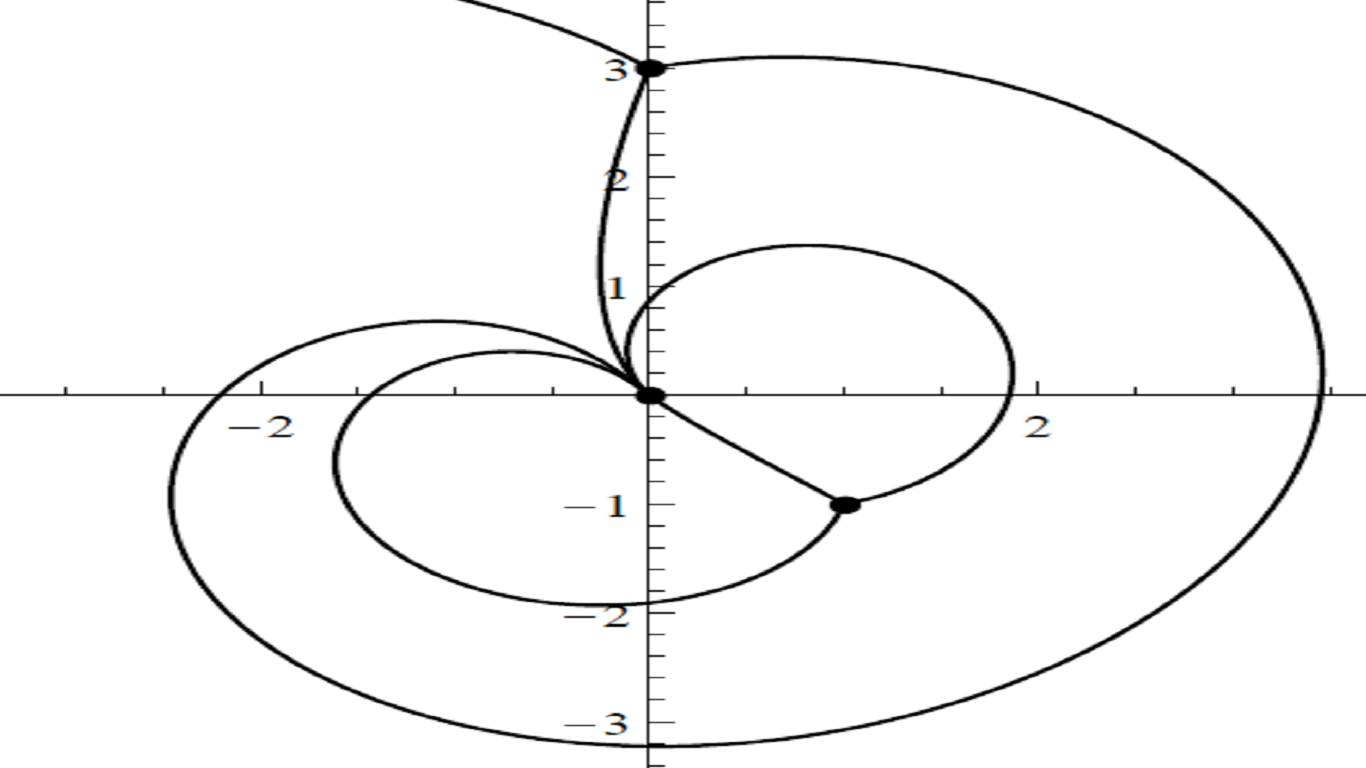
    Figure 3: $\theta_{0}=2\pi$ and $\theta=\frac{2\pi}{3}.$ Here $\lambda^{2}=-2-i,a=3i,b=1-i.$

We just proved the following

Lemma 6

If $\Re\left(\lambda\right)\neq 0,$ then there exists always a critical trajectory of $\varpi\left(\lambda,a,b,z\right)$ diverging to infinity; if there are two, then they emanate from different zeros.

Proof of Proposition 2. Suppose that $\Re\left(\frac{\lambda\left(\sqrt{a}+\sqrt{b}\right)^{2}}{\sqrt{ab}}\right)=0$ and there is no short trajectory connecting $a$ and $b.$ The idea of the proof is to construct two paths $\gamma_{1}$ and $\gamma_{2}$ joining $a$ and $b,$ not homotopic in $\mathbb{C}^{\ast},$ and such that

$$\Im\int_{\gamma_{1}}\dfrac{\lambda\sqrt{\left(z-a\right)\left(z-b\right)}}{z^{2}}dz\neq 0,\Im\int_{\gamma_{2}}\dfrac{\lambda\sqrt{\left(z-a\right)\left(z-b\right)}}{z^{2}}dz\neq 0,$$

which contradicts Proposition 3 and the fact that $\Re\left(\frac{\lambda\left(\sqrt{a}+\sqrt{b}\right)^{2}}{\sqrt{ab}}\right)=0,$ see examples in [15],[16].

We first assume that $\Re\left(\lambda\right)=0.$

There emanate from a zero of $\varpi\left(\lambda,a,b,z\right)$, for example $a,$ two critical trajectories forming a loop $\Omega$ around $\infty$ (in $\overline{\mathbb{C}}$), the third one, say $\gamma_{a}$, diverges to $0.$ The interior angle of the loop $\Omega$ at the vertice $a$ equals $\frac{4\pi}{3}$; applying Lemma 5, we get

$$-1=2+\sum n_{i},$$

it follows that $\Omega$ contains $0$ and $b$ inside, and then, all critical trajectories emanating from $b$ stay in $\Omega.$ Again with Lemma 5, there cannot exist a loop passing through $b,$ and then, we have 4 trajectories that diverge to $0$. Assume that 3 trajectories emanating from $b$ diverge to $0$ in the same direction, then two of them form, with the origin, a domain $\Omega_{b}$ not intersecting $\gamma_{a}$. In this case, all trajectories inside $\Omega_{b}$ diverge to the origin in the same direction, which is impossible (see [14, Theorem7.4]). Then, there are exactly two trajectories $\gamma_{b}^{1}$ and $\gamma_{b}^{2}$ emanating from $b$, and diverging to the origin in the same direction of $\gamma_{a}$. Consider a point $c\in\gamma_{a}$ close to $0$, in a way that the two rays of the orthogonal trajectory $\gamma_{c}^{\perp}$ passing through $c,$ tend to the origin in opposite directions, and then, it intersects $\gamma_{b}^{1}$ and $\gamma_{b}^{2}$ in $b_{1}$ and $b_{2}.$ See Figures 5,5.

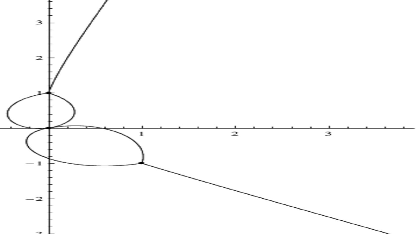
Figure 4: Critical orthogonal trajectories of $\ \varpi\left(i,1-i,i,z\right).$

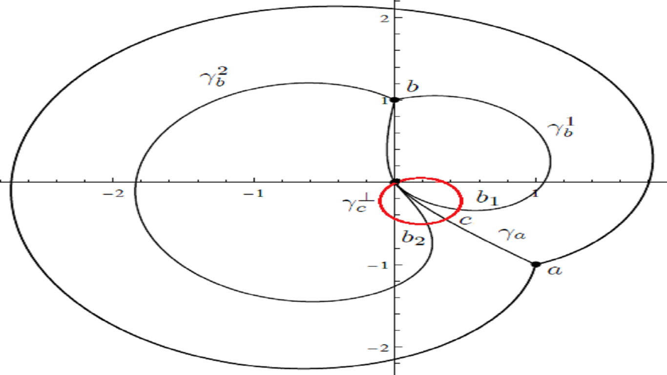
Figure 5: Critical graph of $\varpi\left(i,1-i,i,z\right),$ and the paths $\gamma_{1}$ and $\gamma_{2}.$

Finally, set

• $\gamma_{1}$: the path formed the part of $\gamma_{b}^{1}$ from $b$ to $b_{1},$ the part of $\gamma_{c}^{\perp}$ from $b_{1}$ to $c,$ and, the part of $\gamma_{a}$ from $c$ to $a.$

• $\gamma_{2}$: the path formed the part of $\gamma_{b}^{1}$ from $b$ to $b_{2},$ the part of $\gamma_{c}^{\perp}$ from $b_{2}$ to $c,$ and, the part of $\gamma_{a}$ from $c$ to $a.$

Clearly

$$\Im\int_{\gamma_{1}}\dfrac{\lambda\sqrt{\left(z-a\right)\left(z-b\right)}}{z^{2}}dz =\Im\int_{b_{1}}^{c}\dfrac{\lambda\sqrt{\left(z-a\right)\left(z-b\right)}}{z^{2}}dz\neq 0;$$

$$\Im\int_{\gamma_{2}}\dfrac{\lambda\sqrt{\left(z-a\right)\left(z-b\right)}}{z^{2}}dz =\Im\int_{b_{2}}^{c}\dfrac{\lambda\sqrt{\left(z-a\right)\left(z-b\right)}}{z^{2}}dz\neq 0,$$

which gives the result.

The case $\Re\left(\lambda\right)\neq 0$ is in the same vein since from Lemma 6, there are at list 4 critical trajectories diverging to the origin.   

Proposition 7

If equation (2) admits a real mother-body measure $\mu$, then:

• for some choice of the square root, $p+\sqrt{p^{2}-4r}\in\mathbb{R}.$

• any connected curve in the support of $\mu$ coincides with a short trajectory of the quadratic differential

  $$\varpi=-\frac{D\left(z\right)}{z^{4}}dz^{2},$$ (4)

  where $D\left(z\right)=\left(p^{2}-4r\right)z^{2}+2pqz+q^{2}$ is the discriminant of the quadratic equation (2).

Proof of Proposition 7. Solutions of (2) as a quadratic equation are

$$\mathcal{C}^{\pm}\left(z\right)=\frac{pz+q\pm\sqrt{D\left(z\right)}}{2z^{2}},$$

with some choice of the square root. If $\mu$ is a real mother-body measure of (2), then, its Cauchy transform $\mathcal{C}_{\mu}$ is defined in $\mathbb{C}\setminus$supp$\left(\mu\right)$ by

$$\mathcal{C}_{\mu}\left(z\right)=\int_{\mathbb{C}\setminus\text{\emph{supp}}\left(\mu\right)}\frac{d\mu\left(t\right)}{z-t};$$

it satisfies:

$$\mathcal{C}_{\mu}\left(z\right)=\frac{\mu\left(\mathbb{C}\right)}{z}+\mathcal{\allowbreak O}\left(z^{-2}\right),z\rightarrow\infty;$$ (5)

$$\mathcal{C}_{\mu}\left(z\right)\text{ is analytic in }\mathbb{C}\setminus\emph{supp}\left(\mu\right);$$ (6)

$$\mu=\frac{1}{\pi}\frac{\partial\mathcal{C}_{\mu}}{\partial\overline{z}}.$$

From the equality

$$\mathcal{C}_{\mu}^{\pm}\left(z\right)=\frac{p\pm\sqrt{p^{2}-4r}}{2z}+\mathcal{\allowbreak O}\left(z^{-2}\right),z\rightarrow\infty,$$

we conclude that $\frac{p\pm\sqrt{p^{2}-4r}}{2}=\mu\left(\mathbb{C}\right).$

Since the Cauchy transform $\mathcal{C}_{\mu}\left(z\right)$ of the positive measure $\mu$ coincides a.e. in $\mathbb{C}$ with an algebraic solution of the quadratic equation (2), it follows that the support of this measure is a finite union of semi-analytic curves and isolated points, see [13, Theorem 1]. Let $\gamma$ be a connected curve in the support of $\mu.$ For $t\in\gamma,$ we have

$$\mathcal{C}_{\mu}^{+}\left(t\right)-\mathcal{C}_{\mu}^{-}\left(t\right)=\frac{\sqrt{D\left(t\right)}}{t^{2}}$$

From Plemelj-Sokhotsky’s formula, we have

$$\frac{1}{2\pi i}\left(\mathcal{C}_{\mu}^{+}\left(t\right)-\mathcal{C}_{\mu}^{-}\left(t\right)\right)dt\in\mathbb{R}^{\ast},t\in\gamma,$$

and then we get

$$-\frac{D\left(t\right)}{t^{4}}dt^{2}>0,t\in\gamma,$$

which shows that $\gamma$ is a horizontal trajectory of the quadratic differential (4).

Since the Cauchy transform $\mathcal{C}_{\mu}\left(z\right)$ is well defined and analytic in $\mathbb{C}\setminus$supp$\left(\mu\right),$ it follows that supp$\left(\mu\right)$ should contain all branching points (zeros) of (4). Thus, any connected curve in the support of $\mu$ is a short trajectory of the quadratic differential (4).

For the proofs of the general cases, we refer the reader to [2], [11],[17],[18].   

3 Connection with Bessel polynomials $B_{n}^{\left(\alpha\right)}$

Bessel polynomials $B_{n}^{\left(\alpha\right)}$ are given explicitly by (see [9])

$$B_{n}^{\left(\alpha\right)}\left(z\right)=\sum_{k=0}^{n}\binom{n}{k}\left(n+k+\alpha-2\right)^{\left(k\right)}z^{k},$$ (7)

where $\binom{n}{k}$ is a binomial coefficient, and $\left(x\right)^{\left(k\right)}$ as usual, means $x(x-1)...(x-k+1)$. Equivalently, these polynomials can also be given by the Rodrigues formula

$$B_{n}^{\left(\alpha\right)}\left(z\right)=z^{2-\alpha}e^{\frac{1}{z}}\frac{d}{dz^{n}}\left(z^{2n+\alpha-2}e^{-\frac{1}{z}}\right)$$

Clearly, polynomials $B_{n}^{\left(\alpha\right)}$ are entire functions of the complex parameter $\alpha$. These polynomials fulfill the following three term recurrence relation and second degree differential equation

$$(n+\alpha-1)(2n+\alpha-2)B_{n}(z)$$

$$=((2n+\alpha)(2n+\alpha-2)z+\alpha-2)(2n+\alpha-1)B_{n}(z)+n(2n+\alpha)B_{n-1}(z),$$ (8)

$$z^{2}B_{n}^{\prime\prime}(z)+(\alpha z+1)B_{n}^{\prime}(z)-n\left(n+\alpha-1\right)B_{n}(z)=0,\ n\geq 1.$$ (9)

A non-trivial asymptotic behavior can be obtained in the case of varying coefficients. Namely, we will consider the sequences

$$B_{n}^{(\alpha_{n})},\quad\alpha_{n}/n\underset{n\rightarrow\infty}{\longrightarrow}A,$$

where $A$ is fixed with assumption

$$A\in\mathbb{C}\setminus\left\{-1,-2\right\}.$$ (10)

With each $B_{n}$ in (7) we can associate its normalized root-counting measure

$$\mu_{n}=\mu\left(B_{n}\right)=\frac{\sum_{B_{n}\left(a\right)=0}\delta_{a}}{n},$$

where $\delta_{a}$ is the Dirac measure supported at $a$ (the zeros are counted with their multiplicity). The Cauchy transform of $\mu_{n}$ is given by

$$\mathcal{C}_{\mu_{n}}\left(z\right)=\frac{B_{n}^{\prime}\left(z\right)}{nB_{n}\left(z\right)},B_{n}\left(z\right)\neq 0.$$ (11)

Combining (8) and (9), and reasoning like in [3] (and references therein), we get the following algebraic equation

$$z^{2}\mathcal{C}_{\mu}^{2}\left(z\right)+\left(Az+1\right)\mathcal{C}_{\mu}\left(z\right)-A-1=0.$$ (12)

In this case

$$\mathcal{C}_{\mu}\left(z\right)=\frac{-\left(Az+1\right)+\sqrt{D_{A}\left(z\right)}}{2z^{2}},$$

where

$$D_{A}\left(z\right) =(A+2)^{2}z^{2}+2Az+1$$

$$=(A+2)^{2}\left(z-\left(\frac{1-i\sqrt{A+1}}{A+2}\right)^{2}\right)\left(z-\left(\frac{1+i\sqrt{A+1}}{A+2}\right)^{2}\right).$$

Observe that since $\mathcal{C}_{\mu}\left(z\right)$ satisfies properties (5) and (6), then

• 
  

  the branch of the square root $\sqrt{D_{A}\left(z\right)}$ must be chosen with condition

  $$\sqrt{D_{A}\left(z\right)}\sim(A+2)z,z\rightarrow\infty;$$

• it follows from the behavior of $\mathcal{C}_{\mu}\left(z\right)$ at $z=0$ :

  $$\frac{-\left(Az+1\right)+\sqrt{D_{A}\left(z\right)}}{2z^{2}}=\allowbreak\left(\frac{\sqrt{D_{A}\left(0\right)}}{2}-\frac{1}{2}\right)\left(\frac{1}{z^{2}}+\frac{A}{z}\right)+\mathcal{O}\left(1\right),z\rightarrow 0\allowbreak,$$

  that $\sqrt{D_{A}\left(0\right)}=1.$ This condition gives a precious information about the homotopic class in $\mathbb{C}^{\ast}$ of the short trajectory. See [15, Lemma 2].

The quadratic differential associated to equation (12) is

$$\varpi_{A}=-\frac{D_{A}\left(z\right)}{z^{4}}dz^{2}.$$

Straightforward calculations show that the zeros $\zeta_{-}$ and $\zeta_{+}$ of $D_{A}\left(z\right)$ satisfy

$$\left(A+2\right)\frac{\left(\sqrt{\zeta_{-}}\pm\sqrt{\zeta_{+}}\right)^{2}}{\sqrt{\zeta_{-}\zeta_{+}}}\in 4\left\{1,-A-1\right\}.$$

From Proposition 2, the quadratic differential $\varpi_{A}$ has two short trajectories, when $A\in\mathbb{R}\setminus\left\{-2,-1\right\}$ (see Figures 10,10), otherwise, it has exactly one short trajectory (see Figures 10,10,10).

Laguerre polynomials $L_{n}^{\alpha}\left(z\right)$ can be given explicitly respectively by (see [8]):

$$L_{n}^{(\alpha)}(z)=\sum_{k=0}^{n}\binom{n+\alpha}{n-k}\frac{(-z)^{k}}{k!},$$ (13)

The asymptotic distribution of their zeros and asymptotics was studied in [1],[3],[15]. The key feature in the study of the weak asymptotic is the so-called Gonchar-Rakhmanov-Stahl (GRS) theory [7],[10]. The strong uniform asymptotics on the whole plane are obtained by means of the Riemann–Hilbert steepest descent method of Deift-Zhou [6].

Generalized Bessel polynomials $B_{n}^{(\alpha)}$ are linked to rescaled generalized Laguerre polynomials by

$$B_{n}^{(\alpha)}(z)=z^{n}L_{n}^{(-2n-\alpha+1)}\left(\frac{2}{z}\right)\,.$$

The asymptotic distribution of their zeros and weak and strong asymptotics can be derived by replacing $A\mapsto-(A+2)$ and $z\mapsto 2/z$. In particular, if $A\notin\mathbb{R}$ and $\gamma_{A}$ is the unique short trajectory of $\varpi_{A}$, then, the sequence $\left(\mu_{n}\right)_{n}$ weakly converges to the measure $\mu$ absolutely continuous with respect to the arc-length measure :

$$d\mu\left(z\right)=\frac{1}{2\pi}\frac{\left(\sqrt{D_{A}\left(z\right)}\right)_{+}}{z^{2}}dz.$$

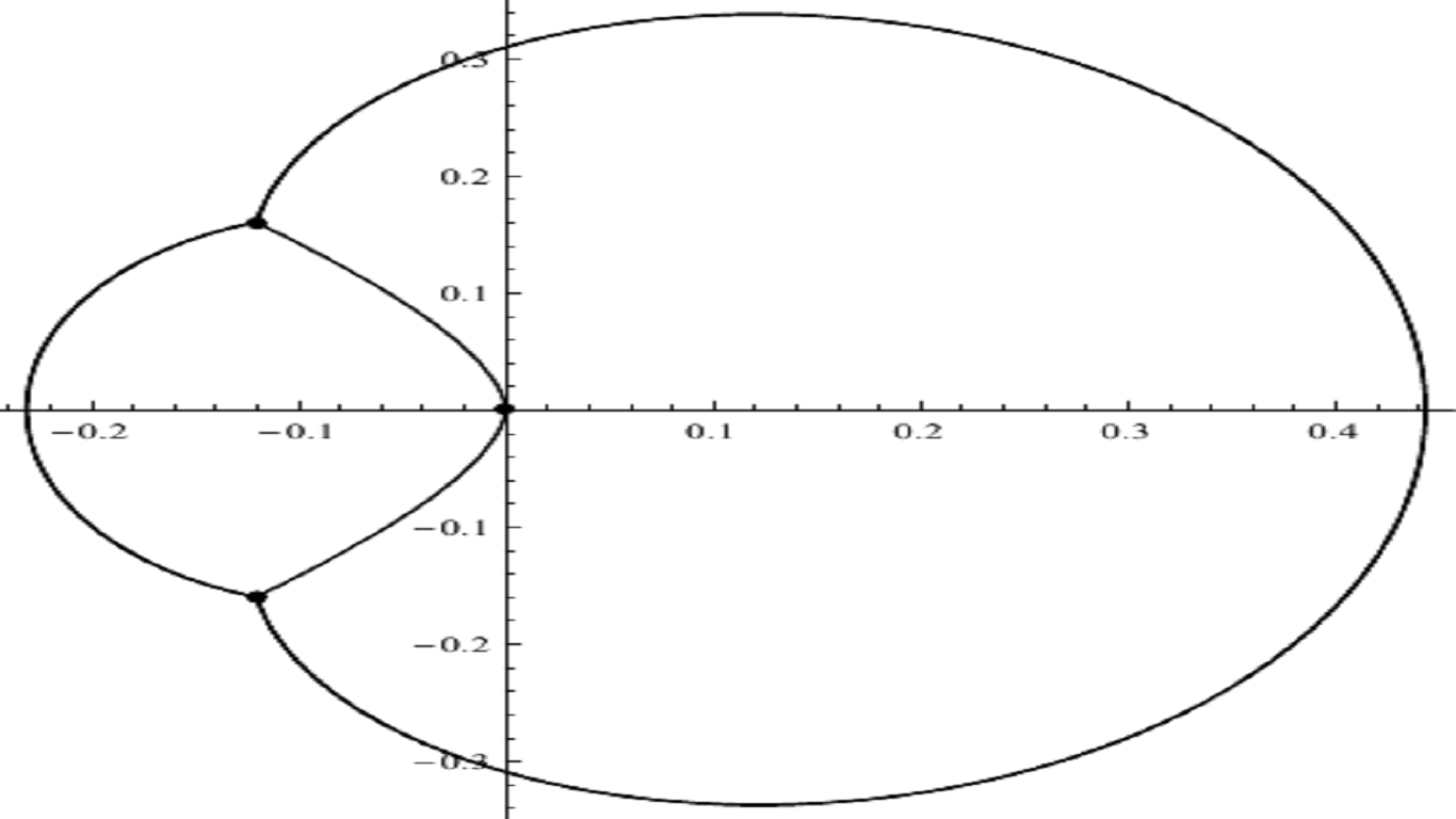
Figure 6:  Critical graph of $\varpi_{3}.$

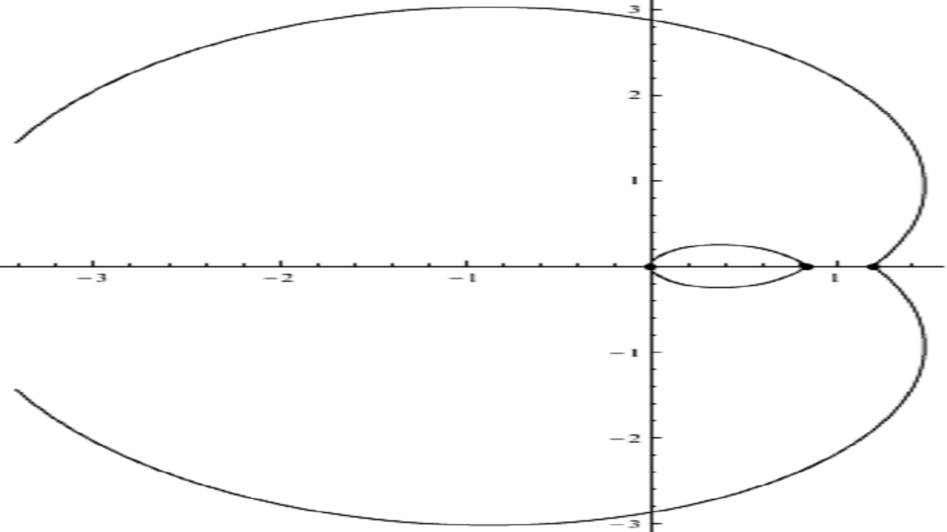
Figure 7: Critical graph of $\varpi_{-1.01.}$

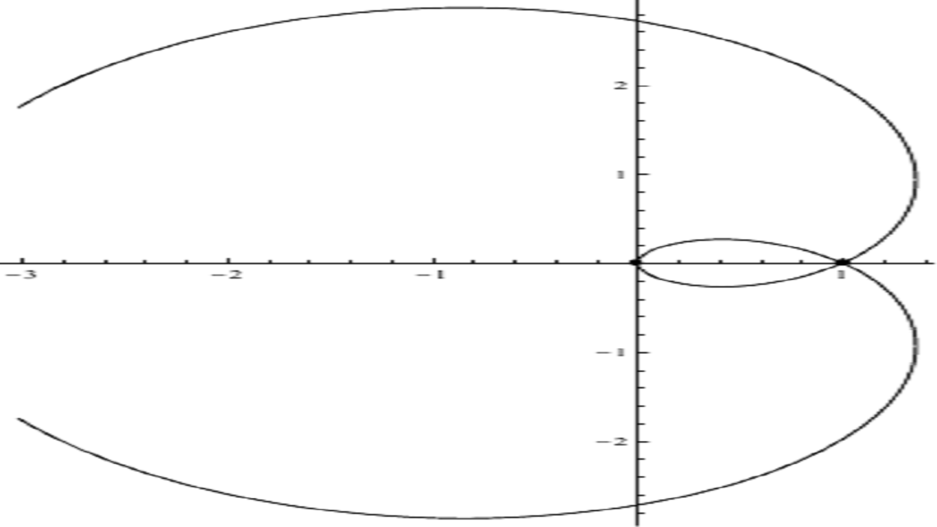
Figure 8: Critical graph of $\varpi_{-1}.$

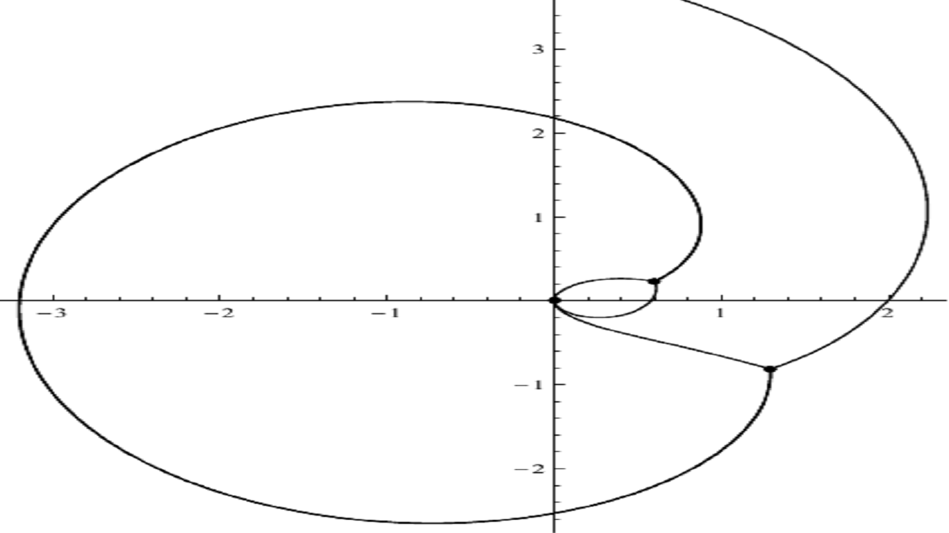
Figure 9: Critical graph of $\varpi_{-1+0.1i}.$

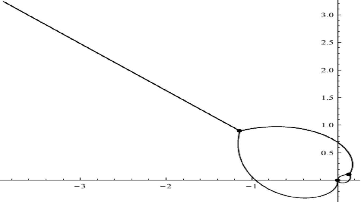
Figure 10: Critical graph of $\varpi_{-2+2i}.$

Acknowledgement 8

The authors have been partially supported by the research unit UR11ES87 from the University of Gabès in Tunisia.

.

Mohamed Jalel Atia(jalel.atia@gmail.com),

Faculté des sciences de Gabès,

Cité Erriadh Zrig 6072. Gabès. Tunisia.

Faouzi Thabet(faouzithabet@yahoo.fr),

Institut Supérieur des Sciences Appliquées

et de Technologie, Avenue Omar Ibn El Khattab 6029.

Gabès. Tunisia.

References

- [1] A. B. J. Kuijlaars, K. T.-R. McLaughlin, Asymptotic zero behavior of Laguerre polynomials with negative parameter, Constructive Approximation 20 (4) (2004) 497-523. Zbl 1069.33008, MR2078083.
- [2] A. Martínez-Finkelshtein, E. A. Rakhmanov, Critical measures, quadratic differentials, and weak limits of zeros of Stieltjes polynomials, Commun. Math. Phys. vol. 302 (2011) 53-111.
- [3] A. Martínez-Finkelshtein, P. Martínez-Gonzalez, R. Orive, On asymptotic zero distribution of Laguerre and generalized Bessel polynomials with varying parameters, J. Comp. Appl. Math. 133 (2001), 477–487. Zbl 0990.33009, MR1858305.
- [4] A. Vasil’ev, Moduli of families of curves for conformal and quasiconformal mappings, Vol. 1788 of Lecture Notes in Mathematics, Springer-Verlag, Berlin, 2002. Zbl 0999.30001, MR1929066.
- [5] C. Pommerenke, Univalent Functions, Vandenhoeck & Ruprecht, Göttingen, 1975. With a chapter on quadratic differentials by Gerd Jensen; Studia Mathematica/Mathematische Lehrbücher, Band XXV. Zbl 0298.30014, MR0507768.
- [6] Deift, P.A.: Orthogonal polynomials and random matrices: a Riemann-Hilbert approach. New York University Courant Institute of Mathematical Sciences, New York (1999). (MR2000g:47048).
- [7] Gonchar, A.A., Rakhmanov, E.A.: Equilibrium distributions and degree of rational approximation of analytic functions. Math. USSR Sbornik 62(2), 305–348 (1987). (translation from Mat. Sb., Nov. Ser.134(176), No.3(11), 306–352 (1987))
- [8] G. Szego, Orthogonal polynomials, fourth ed., Amer. Math. Soc. Colloq. Publ., vol. 23, Amer. Math. Soc., Providence, RI, 1975.
- [9] H. L. Krall and Orrin Frink, A New Class of Orthogonal Polynomials: The Bessel Polynomials, Transactions of the American Mathematical Society Vol. 65, No. 1 (Jan., 1949), pp. 100-115.
- [10] H. Stahl, Orthogonal polynomials with complex-valued weight function. I,II, Constr. Approx. 2 (1986), no. 3, 225–240, 241–251. MR 88h:42028.
- [11] Igor E. Pritsker. How to find a measure from its potential. Computational Methods and Function Theory, Volume 8 (2008),No.2, 597-614.
- [12] J. A. Jenkins, Univalent functions and conformal mapping, Ergebnisse der Mathematik und ihrer Grenzgebiete. Neue Folge, Heft 18. Reihe: Moderne Funktionentheorie, Springer-Verlag, Berlin, 1958. Zbl 0083.29606, MR0096806.
- [13] J.-E. Bjork, J. Borcea, R.Bőgvad, Subharmonic Configurations and Algebraic Cauchy Transforms of Probability Measures. Notions of Positivity and the Geometry of Polynomials Trends in Mathematics 2011, pp 39-62.
- [14] Kurt Strebel, Quadratic differentials, Ergebnisse der Mathematik und ihrer Grenzgebiete (3) [Results in Mathematics and Related Areas (3)], vol. 5, Springer-Verlag, Berlin, 1984. Zbl 0547.30001, MR8630072.
- [15] M. J. Atia, A. Martínez-Finkelshtein, P. Martínez-Gonzalez, and F. Thabet, Quadratic differentials and asymptotics of Laguerre polynomials with varying complex parameters, J. Math. Anal. Appl. 416 (2014), 52–80. Zbl 1295.30015, MR3182748.
- [16] M. J. Atia and F. Thabet, Quadratic differentials A(z-a)(z-b)dz^2/(z-c)^2 and algebraic Cauchy transform. arXiv1506.06543v1.To appear in Cze.Jour.Math.
- [17] Rikard Bőgvad and Boris Shapiro, On motherbody measures and algebraic Cauchy transform
- [18] T. Bergkvist and H. Rullgård, On polynomial eigenfunctions for a class of di erential operators. Math. Res. Lett. 9 (2002), 153-171.