Dark Matter Trapping by Stellar Bars: The Shadow Bar

Abstract

We investigate the complex interactions between the stellar disc and the dark-matter halo during bar formation and evolution using N-body simulations with fine temporal resolution and optimally chosen spatial resolution. We find that the forming stellar bar traps dark matter in the vicinity of the stellar bar into bar-supporting orbits. We call this feature the shadow bar. The shadow bar modifies both the location and magnitude of the angular momentum transfer between the disc and dark matter halo and adds 10 per cent to the mass of the stellar bar over 4 Gyr. The shadow bar is potentially observable by its density and velocity signature in spheroid stars and by direct dark matter detection experiments. Numerical tests demonstrate that the shadow bar can diminish the rate of angular momentum transport from the bar to the dark matter halo by more than a factor of three over the rate predicted by dynamical friction with an untrapped dark halo, and thus provides a possible physical explanation for the observed prevalence of fast bars in nature.

1 Introduction

Galactic bars change the internal structure of disc galaxies by rearranging the angular momenta and energy of orbits that would otherwise be conserved. As many as two-thirds of local galaxies show bar features in the infrared (Sheth et al., 2008). Bars have been suggested to affect both structural properties such as bulge structure (Kormendy & Kennicutt, 2004; Laurikainen et al., 2014) and stellar breaks (Muñoz-Mateos et al., 2013; Kim et al., 2014), as well as evolutionary properties such as star formation rates (Masters et al., 2012; Cheung et al., 2013) and metallicity gradients (Williams et al., 2012). Weinberg & Katz (2002) also showed that bars can affect the central profiles of dark matter haloes. Bars are the strongest of the persistent disc asymmetries and, therefore, provide a dynamical laboratory for understanding the long-term evolution of galaxies.

For simplicity of analysis, many previous theoretical works have adopted a component-by-component analysis of angular momentum transport by adopting a fixed halo potential, a rigid bar, or both. However, the baryonic disc and dark matter halo comprise a single system that shares the same dynamics as a consequence of their mutually generated gravitational field. Therefore, some fraction of the dark-matter orbital elements will overlap with those in the disc and, thus, there is little reason not to suspect that some of the dark matter halo will respond similarly to the stellar disc. The dynamical interplay between these components is of considerable interest in developing a comprehensive understanding of the disc-halo system.

In this paper, we present a time-dependent analysis of trapped stellar and halo orbits in a fully self-consistent simulation. We find evidence for the formation and subsequent secular evolution of a trapped population of halo orbits, a shadow bar, that arises in response to the same collective dynamics that make the classic stellar bar. The shadow bar fundamentally changes the orbital structure of the halo in the vicinity of the bar. These same orbits, when unperturbed by the bar, would contribute strongly to the disc-halo torque responsible for slowing the bar, which can be understood in the context of simple perturbation theory models. We investigate and document the magnitude of halo trapping, finding that the trapping affects both the dark-matter density and velocity structure.

A well-studied consequence of angular momentum transport in barred galaxies is the tension between the theorised slowing of the bar pattern speed (Tremaine & Weinberg, 1984; Weinberg, 1985) and observations that do not show a slowing pattern speed (e.g. Aguerri et al. 2015). This is often interpreted as evidence for only small amounts of dark matter at the centre of galaxies (Debattista & Sellwood, 2000; Sellwood & Debattista, 2006; Villa-Vargas et al., 2009) or as a motivation for changing the law of gravity (Tiret & Combes, 2007). However, the dark-matter orbits trapped by the bar are unavailable for secular evolution, significantly reducing the halo torque on the bar.

For our own Milky Way (MW)—a barred galaxy—several experiments may detect the influence of a shadow-bar modified dark matter density and velocity distribution. These include ongoing analysis of stellar surveys such as RAVE (Steinmetz et al., 2006), GAIA (Gilmore et al., 2012), and APOGEE (Allende Prieto et al., 2008) since halo stars might have similar orbits to dark matter particles. Some of these studies have already seen suggestions of rotation in a bulge-bar component (Rojas-Arriagada et al. 2014, Soto et al. 2014). Signs of a shadow bar could also affect the interpretation of tentative signals from direct dark matter detection experiments, e.g. CoGeNT (Aalseth et al., 2013), CDMS II (Agnese et al., 2013), and DAMA/LIBRA (Bernabei et al., 2014).

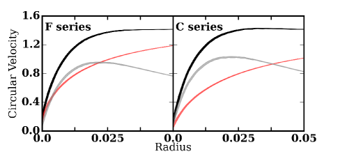
Figure 1: Initial circular velocity curves for the F-series cusp models (left panel) and C-series cored models (right panel). The circular velocity from $p=0.2$ to $p=0.8$ is shown in black where $p$ is the quantile value for the rank-ordered circular velocities. The $p=0.2$ to $p=0.8$ contributions from the disc (grey line) and halo (red line) have been separated to demonstrate the maximality of the disc. Radius and circular velocity are in virial units (see Section 2.1), where a radius of $0.01$ coresponds to $3$ kpc and a circular velocity of $1.0$ corresponds to 150 km s^-1 when scaled to a Milky Way mass galaxy.

This paper is organised as follows: the next section describes the initial conditions for our fiducial simulation (section 2.1.1), a series of simulations with varying halo properties (section 2.1.2), and the details of our N-body solver (section 2.2). We include two idealised numerical experiments with modifications to the bar perturbation to better understand the importance of the bar growth rate on halo orbit trapping and halo structure. Our results are presented in section 3. We examine the fiducial simulation in detail, beginning with an overall summary picture of the fiducial simulation in section 3.1, followed by studies of the disc and halo orbit morphologies in sections 3.2.1 and 3.2.2, respectively. These analyses reveal that in addition to the stellar bar, a significant mass fraction of the halo within a bar length is trapped into the bar potential. The dynamical properties of the entire trapped orbit population are discussed in section 3.3 and contextualised using perturbation theory. This is followed by an exploration of the overall dynamical consequences of the shadow bar itself in section 3.4. Section 4 connects with previous work by using a suite of experiments motivated by published models and further demonstrates the robust nature of the shadow bar. We conclude with a summary and discussion of the stellar disc–dark matter halo relationship and our detailed orbital analysis in section 5.

2 Methods

2.1 Initial conditions

This section motivates our mass models and describes the realisation of the initial conditions. We begin with the details of our fiducial simulation. The phase space is realised using a methodology that closely follows Holley-Bockelmann et al. (2005), hereafter HB05. We then discuss model variants that (1) address typical literature treatments; (2) seek to model physical processes in the universe; and (3) verify the theorised dynamical implications of the fiducial experiment. Our key simulations are summarised in Table 1.

In all the simulations presented here, the number of disc particles and halo particles are $N_{\rm disc}=10^{6}$ and $N_{\rm halo}=10^{7}$, respectively. The disc particles have equal mass. The halo particles have a number density $n_{\rm halo}\propto r^{-\alpha}$, where $\alpha=2.5$. This steep power law better resolves the inner halo in the vicinity of the disc bar, our subject of interest. The particle’s masses are assigned to simultaneously reproduce the desired halo mass density and the number density. In practice, the halo resolution is improved by a factor of 100 within a disc scale length ($M_{r<R_{d}}=0.005M_{\rm vir}$, $N_{r<R_{d}}=5\times 10^{5}$) compared to using a fixed halo particle mass. The effective halo particle number within all disc-relevant radii is then $N_{\rm halo}\sim 10^{9}$, more than satisfying the criteria of Weinberg & Katz (2007b) for an adequate treatment of resonant dynamics.

All units are scaled to so-called virial units with $G=1$ that describe the mass and radius of the halo at the point of halo collapse in the cold-dark-matter scenario. For comparison to the MW, we follow the estimated halo mass of Boylan-Kolchin et al. (2013) such that $M_{\rm vir}=1.6\times 10^{12}~{}{\rm M}_{\odot}$, making $R_{\rm vir}=1.0$ correspond to 300 kpc, a velocity of 1.0 equivalent to 150 km s^-1, and a time of 1.0 equivalent to 2.0 Gyr. The system is constructed such that $M(R_{\rm vir})=1.0$.

2.1.1 Fiducial simulation

We follow the now standard prescription for producing a strong bar in an N-body simulation by choosing a fiducial model with a slowly rising rotation curve. This simulation is labelled F in Table 1, using the initial rotation curve shown by the F-series rotation curve in Fig. 1 (left panel). The contributions from the individual components are derived by calculating the radial force contributions from each component separately: $v_{c,{\rm disc}}^{2}=rF_{r,{\rm disc}}$ and $v_{c,{\rm halo}}^{2}=rF_{r,{\rm halo}}$ where $r$ is the radius of the particle, and $F_{r}$ is the radial force contribution from the corresponding component at the particle’s position. The slowly rising rotation curve minimises the bar-damping effect of the initial inner Lindblad resonance and allows the region inside of corotation to act as a “resonant cavity” for bar formation (Sellwood & Wilkinson, 1993). For a rising rotation curve, one can show using first-order perturbation theory that the response of a nearly circular orbit to the bar perturbation is to slow and even reverse its apse precession rate (the so-called “donkey effect” of Lynden-Bell & Kalnajs 1972, see Binney & Tremaine 2008). This results in the orbit lingering near the position angle of the bar, causing the effective bar strength, the quadrupole perturbation strength specifically, to increase. This growth extends the reach of the perturbation, inducing more orbits to slow or reverse their precession rate, resulting in an exponential growth for the bar. The fiducial simulation is analysed in section 3.

The fiducial simulation has an initially exponentially-distributed stellar disc embedded in a fully self-consistent non-rotating $c=R_{\rm vir}/r_{s}\approx 15$ NFW dark-matter halo (Navarro et al., 1997) where $r_{s}$ is the scale radius, and $R_{\rm vir}$ is the virial radius:

$$\rho(r)=\frac{\rho_{0}r_{s}^{3}}{(r+r_{c})(r+r_{s})^{2}}$$ (1)

where $\rho_{0}$ is set by the chosen mass and $r_{c}=0$ is the core radius for the fiducial model. The dynamical implications of a core produced by early evolutionary processes (Weinberg & Katz 2002, Sellwood & Debattista 2009) will be explored in section 3 and 4 by comparison to simulations with non-zero values of $r_{c}$. The halo velocities are realised from the distribution function produced by an Eddington inversion of $\rho(r)$ (see Binney & Tremaine 2008). Eddington inversion provides an isotropic distribution, roughly consistent with the observed distributions in dark-matter only $\Lambda$CDM simulations. This method naturally results in a non-rotating halo; we will describe realising rotating haloes in section 2.1.2.

For all the simulations here, we adopt an exponential radial stellar disc profile with an isothermal vertical distribution:

$$\rho_{d}(R,z)=\frac{M_{\rm d}}{8\pi z_{0}R_{d}^{2}}e^{-R/R_{d}}{\rm sech}^{2}(z/z_{0})$$ (2)

where $M_{d}$ is the disc mass, $R_{d}$ is the disc scale length, and $z_{0}$ is the disc scale height. We set $M_{d}=0.025$, $R_{d}=0.01$, and $z_{0}=0.001$ throughout. All simulations in this work have a disc:halo mass ratio of 1:40 inside of its virial radius; while a comparatively low mass ratio for studies in the literature (e.g. contrasting with Debattista & Sellwood 2000; Athanassoula & Misiriotis 2002; Saha et al. 2012), we choose this mass ratio to mimic the mass ratio for the $z=0$ MW, as determined through simulations (Vogelsberger et al., 2014), abundance matching (Kravtsov 2013; Moster et al. 2013), and stellar kinematics (Bovy & Rix, 2013). The disc parameter values are consistent with the MW values of Bovy & Rix (2013), who found $M_{\star}\approx 4.6\times 10^{10}$, or $0.029~{}M_{\rm vir}$ (again using the scaling from Boylan-Kolchin et al. 2013); $R_{d}=2.15$ kpc and $z_{0}=370$ pc, which are reasonably similar to our values. We do not include a bulge due to the uncertainty in its phase-space distribution, but this should not limit the application of our models to the observed universe since the dynamical mechanisms governing bar formation and evolution are dominated by the graviatational potential outside the bar region. Similarly for the thick disc, although we will address the dynamical effects of a thick disc in a later paper. We additionally do not include a gas component. In the present-day, gas is a tracer component in the MW; while the gas fraction may have been higher in the past, this quantity is highly uncertain. Literature results have demonstrated scenarios where gas accretion can destroy and re-form the bar over a cosmological (Bournaud & Combes, 2002; Bournaud et al., 2005). However, other simulations including gas as part of the initial conditions (Villa-Vargas et al., 2010; Athanassoula et al., 2013) do not show signs of bar destruction, though the bars resulting from gas-rich simulations may be weaker. While including gas as part of the initial conditions may slow the rate at which bars form, the presence of a gas component does not fundamentally alter the dynamics. In light of this, we suggest that our models are adequate for learning about the dynamical mechanism of DM trapping, and believe that the results presented here would remain largely unchanged in the presence of a collisional component with present-day parameters.

The F-series rotation curve has a disc fraction $f_{D}\equiv V_{c,\star}/V_{c,{\rm tot}}=0.71$ at $R=2.2R_{d}$, the radius at which the exponential disc reaches the maximum circular velocity. Martinsson et al. (2013) found that for typical spiral galaxies, $f_{D}=0.4-0.7$, with $\langle f_{D}\rangle=0.57$, making our disc more maximal than the typical spiral. Piffl et al. (2014) measured $f_{D}=0.63$ for the MW, in agreement with the findings of Martinsson et al. (2013). However, Bovy & Rix (2013) suggested that the MW may be nearer to a maximal disc, with $f_{D}=0.83$. All methods to observationally determine $f_{D}$ rely on assumptions about the parameters to describe the disc, as well as the structure of the dark matter halo, hence we believe that within the uncertainties, our fiducial model represents a realistic galaxy. The purpose of the simulation was not to create an exact MW analogue, but to make a cosmologically realistic galaxy.

Disc velocities are chosen by solving the Jeans’ equations in cylindrical coordinates in the combined disc–halo potential. We set the radial velocity dispersion from the Toomre stability equation,

$$\sigma_{r}(R)=Q\frac{3.36G\Sigma(R)}{\kappa(R)},$$ (3)

where $G=1$, $\Sigma(R)$ is the stellar surface density, and $\kappa$, the epicyclic frequency (also sometimes written as $\Omega_{r}$), is given by

$$\kappa^{2}(R)=R\frac{d\Omega(R)^{2}}{dR}+4\Omega(R)^{2}$$ (4)

where $\Omega$ is the azimuthal frequency (sometimes explicitly written as $\Omega_{\phi}$ in cylindrical coordinates). We choose $Q=0.9$ to facilitate comparisons to the literature (e.g. Athanassoula & Misiriotis 2002) and to ensure the relatively rapid growth of a bar. This departs from our previous choice in HB05 of a warm disc with $Q=1.4$. Also, we replace the axisymmetric velocity ellipsoid generated from the epicyclic approximation in the disc plane used in HB05 by the Schwarzschild velocity ellipsoid (Binney & Tremaine, 2008). In practice, this latter velocity ellipsoid improves the initial equilibrium by using the second moment of the cylindrical collisionless Boltzmann equation with an asymmetric drift correction:

$$\sigma_{\phi}^{2}=\left(\frac{\sigma_{r}\kappa(R)}{2\Omega(R)}\right)^{2}.$$ (5)

As in HB05, the vertical velocity dispersion $\sigma_{z}$ is

$$\sigma_{z}^{2}(R)=\frac{1}{\rho_{d}(R,z)}\int_{z}^{\infty}\rho_{d}(R,z)\frac{\partial\Phi_{\rm tot}}{\partial z}dz.$$ (6)

From a dynamical standpoint, our relatively low disc-to-halo mass ratio accomplishes two additional goals: (1) it decreases the strength of local instabilities that allows us to focus on secular dynamics; and (2) it enables the exploration of the slow mode of bar growth (Polyachenko & Polyachenko, 1996), seemingly not achievable given maximal discs. We examine the former in this paper and will explore the latter in more detail in a forthcoming paper.

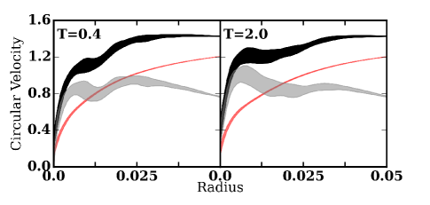
Figure 2: Circular velocity curves for the fiducial model at system time T=0.4 (left panel) and T=2.0 (right panel). The circular velocity from $p=0.2$ to $p=0.8$ is shown in black. The $p=0.2$ to $p=0.8$ contributions from the disc (grey line) and halo (red line), where $p$ is the quantile value for the rank-ordered circular velocities, have been calculated separately to demonstrate the evolution of each component. Radius and circular velocity are in virial units, as in Figure 1. System time is also given in virial units, where T=1.0 corresponds to 2.0 Gyr when scaled to the MW.

Simulation	scale length ($R_{d}$)	scale height ($h$)	disc mass	halo profile	Notes
F	0.01	0.001	0.025	cusp
Fr	0.01	0.001	0.025	cusp, $\lambda=0.03$
C	0.01	0.001	0.025	cored, $r_{c}=0.02$
Cr	0.01	0.001	0.025	cored, $r_{c}=0.02$, $\lambda=0.03$
Ff	0.01	0.001	0.025	cusp	fixed disc potential
Fs	0.01	0.001	0.025	cusp	shuffled halo

Table 1: List of simulations.

2.1.2 Halo model variants

We investigate two additional classes of halo models based on our fiducial one: (1) halo models with a cored central profile instead of a cusp; and (2) rotating haloes. These variants are inspired both by cosmological hydrodynamic simulations (Bullock et al., 2001), and a desire to connect with previous literature choices.

We construct cored haloes by setting $r_{c}=0.02$ in equation (1). The halo mass is matched between the cusp and core model haloes at the virial radius to maintain the disc:halo mass ratio within the virial radius. This model uses the C-series rotation curve (the right panel of Figure 1). The overall rotation curves for the F- and C-series models are within 5 per cent at any given radius, despite the relative contributions from each component being appreciably different. The C-series rotation curves have $f_{D}=0.81$ at $R=2.2R_{d}$. As we shall see, the resonant dynamics are quite different, as the phase-space gradient of the distribution function is the controlling parameter of the resonant density (see Sellwood 2014 for a review). In a cored halo, the flattening of the central density profile creates a harmonic core, i.e. orbits at small radii would execute simple harmonic motion in the absence of a stellar disc. For this model series, the relatively low halo density near the centre of the simulation leads to a well-known buckling instability (see Sellwood 2014 for a review). The differences between the fiducial and variant halo models are discussed in section 4.1.

We construct rotating haloes consistent with the cumulative mass distribution $M$ for specific angular momentum $j(M)$ in a spherical shell as proposed by Bullock et al. (2001),

$$j(M)\propto M^{1.3},$$ (7)

normalised such that

$$\lambda=\frac{\sum_{i}m_{i}\vec{r_{i}}\times\vec{v_{i}}}{\sqrt{2}M_{\rm vir}V_{\rm vir}R_{\rm vir}}=0.03.$$ (8)

The value $\lambda=0.03$ is roughly the median value in the distribution compiled from cosmological simulations by Bullock et al. (2001). We realise a distribution that satisfies equations (7) and (8) as follows. First, we begin with a phase space for the initially nonrotating spherical halo as described in section 2.1.1. We randomly sample the phase space of the initially nonrotating halo by mass as described in section 2.1.1 and choose particles from the distribution $M(r)$ by rejection. Then, we change the direction of rotation for orbits with $L_{z}<0$ from the probability distribution determined from equation (7) by changing the sign of $L_{z}$ until the desired value of $\lambda$ is obtained. For our $N=10^{7}$ haloes, this results in a deviation from the desired $\lambda=0.03$ of less than 1 per cent. Changing the sign of any component of the angular momentum of a particular orbit remains a valid solution to the collisionless Boltzmann equation, preserving the initial equilibrium of the system. Large values of $\lambda$ may result in an unstable halo (Kuijken & Dubinski, 1994), but this is not observed for the modest $\lambda$ selected here, unsurprising given the results of Barnes et al. (1986) and Weinberg (1991). The initial rotation curves for Fr and Cr (see Table 1) are the F and C series respectively (Figure 1).

2.1.3 Two tests of the dynamical mechanism

In addition to the halo model variants, we examine two additional modifications to the fiducial model designed to test our physical understanding of the dynamical processes. Such restricted simulations do not have analogues in the real universe, but can illuminate specific processes.

In the first experiment, Ff in Table 1, we exploit the separate Poisson-equation solutions for the stellar disc and dark matter halo in EXP (see below for a description of this N-body code) by allowing the dark matter halo potential to self-consistently evolve while disallowing changes to the stellar disc potential. This allows us to investigate the adiabatic compression of the initially spherical dark matter halo in response to the stellar disc potential. The results are compared to that of the fiducial simulation in section 3.2.2 to isolate the effect of non-axisymmetric disc evolution on the global halo properties.

In the second experiment, Fs in Table 1, we artificially eliminate the trapping that leads to the shadow bar by shuffling the azimuth of halo particles in the fiducial simulation. The shuffling interval for an individual orbit $i$ is chosen following a Poisson distribution with an average value of $2P_{\phi,i}$ where $P_{\phi,i}\equiv 2\pi/\Omega_{\phi,i}$ is the azimuthal period for orbit $i$. This technique preserves the radial structure of the halo and produces minimal disturbances to the equilibrium. The results of this experiment are used to quantify the effect of trapping on classical dynamical friction torque and to corroborate our hypothesis of the shadow bar’s effect on the angular momentum transport between the disc and halo in section 3.4.

We verify that the shuffling process effectively eliminates trapping by attempting to detect a trapped component using the methodology that will be described in 3.2, finding that $<$0.1 per cent of the orbits demonstrate a trapped signal, consistent with uncertainties owing to resolution. Both models use the F-series initial rotation curve (Figure 1)

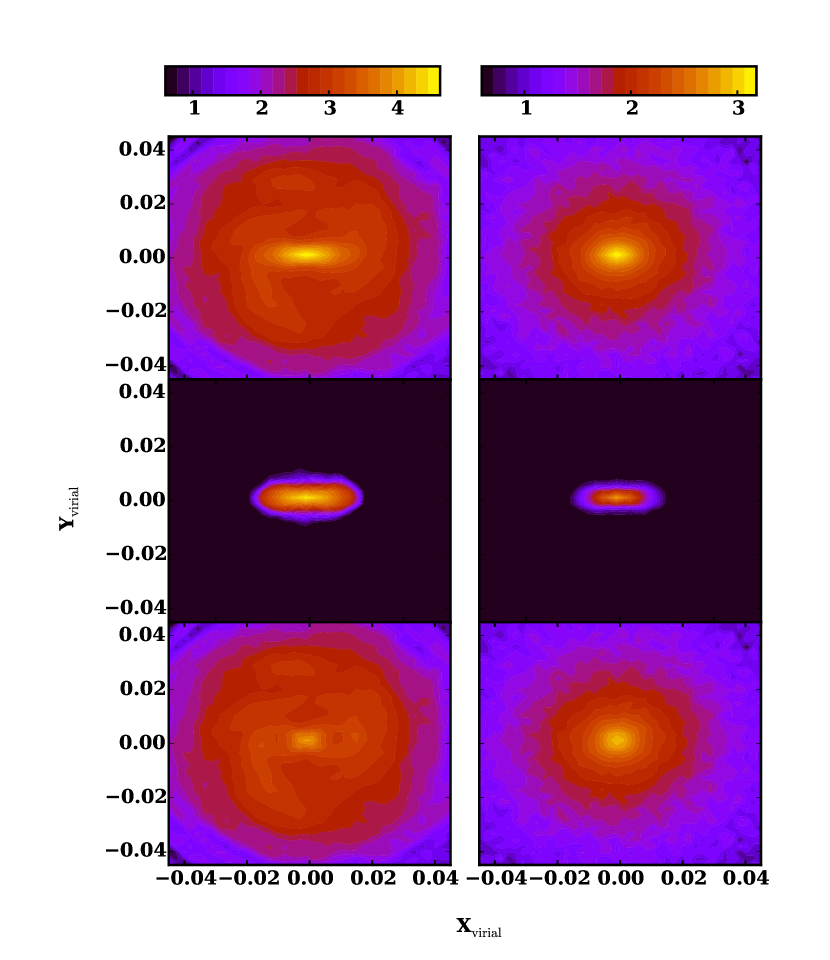
Figure 3: The surface density of the fiducial simulation for the stellar disc (left panels) and the dark matter halo (right panels). The upper panels show the in-plane density ($|z|<0.003$, $\approx$ 1 kpc for MW-like scalings), the middle panels show the in-plane density of the trapped component (the stellar bar on the left and the shadow bar on the right), and the lower panels show the in-plane density of the untrapped component, at T=2.0 (4 Gyr for MW-like scalings). Positions are given in virial units, as in Fig. 1, discussed in section 2.1.

2.2 N-body simulations

We perform the system evolution using EXP (Weinberg, 1999). This code is designed to represent the gravitational field for multiple galaxy components by a rapidly converging series of functions. EXP is advantageous for secular dynamics problems owing to its absence of high-frequency noise and its high-efficiency relative to fully adaptive Poisson solvers such as direct summation or tree gravity algorithms.

These series of functions are the eigenfunctions of the Laplacian. For conic coordinate systems, the Laplacian is a special case of the Sturm-Liouville (SL) equation,

$$\frac{d}{dx}\left[p(x)\frac{d\Phi(x)}{dx}\right]-q(x)\Phi(x)=\lambda\omega(x)\Phi(x)$$ (9)

where $\lambda$ is a constant and $\omega(x)$ is a known function, called either the density or weighting function. These eigenfunctions have many useful properties. For systems with a finite domain, the eigenvalues are real, discrete, and bounded from below; their corresponding eigenfunctions are mutually orthogonal, and oscillate more rapidly with increasing eigenvalue. We will assume that the functions are indexed in order of increasing eigenvalue. For example, the eigenfunctions of the Laplacian over a periodic finite interval are sines and cosines; in cylindrical coordinates, they are Bessel functions. For a spherical geometry, the eigenfunctions satisfy Poisson’s equation such that

$$\frac{1}{4\pi G}\int drr^{2}d^{*}_{k}(r)u_{j}(r)=\delta_{jk}$$ (10)

where $d_{k}$ is the density and $u_{j}$ is the potential that together form a biorthogonal pair. A variety of analytic biorthgonal pairs are available (Clutton-Brock 1973, Clutton-Brock et al. 1977, Hernquist & Ostriker 1992, Earn 1996). Here, we follow Weinberg (1999) and numerically solve equation (9) to obtain a basis whose lowest-order pair ($n=0$, $l=m=0$) matches the equilibrium profile of the initial conditions. Higher-order terms then represent deviations about this profile with successive higher spatial frequency, which can account for the evolution of the system.

The overall power owing to discreteness noise scales as $1/N$, and we may limit small-scale fluctuations by truncating the series, effectively providing a low-pass spatial filter that removes high-frequency noise from the discrete particle distribution (Weinberg, 1998). Although it is possible to derive an analogous three-dimensional basis from the cylindrical Laplacian, the boundary conditions are complex and difficult to match to the approximately spherical domain of the halo. After much trial and error, we found that a empirical orthogonal function decomposition of a high-dimensional spherical basis produces better results. Weinberg (1999) and HB05 describe this method in detail. The field approach is also advantageous as it enables a direct comparison with perturbation theory. However, we are aware of two significant disadvantages of the field approach as well: 1) the technique cannot be fully adaptive and limit high frequencies simultaneously; and 2) it can be susceptible to $m=1$ (dipole) modes induced by unphysical ‘sloshing’ of the expansion centre against the centre-of-mass. While our simulations show nonzero $m=1$ power, we verify that the expansion centre deviates from the centre-of-mass by less than $0.1z_{0}$ at all times. We also note that $m=1$ modes are theoretically predicted (Weinberg, 1994) and appear in real galaxies (e.g. Zaritsky et al. 2013) and hence do not necessarily indicate a numerical fault. We will investigate these phenomena further in a future paper.

For this class of Poisson solver, the computational effort scales linearly with particle number, making low-noise simulations with high $N$ possible. A number of basis terms are kept to allow for astronomically realistic perturbations to the equilibrium profile while minimising the linear least-squares fit to a Monte Carlo realisation of the initial particle positions. We retain terms in the halo basis up to $l=m=6$, and a maximum radial index of $n=20$ corresponding to the largest eigenvalues for the spherical harmonics of the halo. For the disc, we select $m=6$, $n=12$ for the empirical orthogonal functions. This basis selection allows for variations of $0.1R_{d}$ (300 pc for a MW-sized galaxy) in the vicinity of the bar, decreasing to $5\times 10^{-5}$ (15 pc for a MW-sized galaxy) near the centre. This solver naturally suppresses the small scales that may lead to anomolous diffusion, which can lead to unphysically rapid evolution, without adding spatial resolution on the scales of interest. While possible, we do not recondition the basis on the evolving equilibrium during simulations, relying instead on the initial Poisson variance to allow for sufficient degrees of freedom.

Particles are advanced using a leapfrog integrator with an adaptive time step algorithm. Briefly, we begin by partitioning phase space $s$ ways such that each partition contains $n_{j}$ particles that require a time step $\delta t=2^{-j}\delta T$, where $\delta T$ is the largest time step and $j=0,\ldots,s-1$. The time step for $j=s-1$ corresponds to a single time-step simulation. Since the total cost of a time step is proportional to the number of force evaluations, the speed up factor is given by: ${\cal S}=\sum_{j=0}^{s-1}n_{j}/\sum_{j=0}^{s-1}n_{j}2^{-j}$. For a $c=15$ NFW dark-matter profile with $N=10^{7}$ multimass particles as described in section 2.1.1, we find that $s=8$ and ${\cal S}\approx 30$, an enormous speed up! Forces in our algorithm depend on the basis coefficients and the leap frog algorithm requires linear interpolation of these coefficients to maintain second-order error accuracy per step. The expansion coefficients are partially accumulated and interpolated at each level $j$ to preserve continuity as required by the numerical integration scheme for finer time steps. This interpolation and the bookkeeping required for the successive bisection of the time interval is straightforward. The symmetric structure of the leap-frog algorithm allows the coefficient values to be interpolated rather than extrapolated. This algorithm will be discussed in more detail in a forthcoming paper.

To motivate our choice of timesteps, we first define a characteristic force scale as $d_{i}\equiv\Phi_{i}/|\partial\Phi_{i}/\partial\mathbf{x}_{i}|$ where $\Phi_{i}$ is the current scalar potential of the particle. The time step level, $j$, for each orbit is then assigned by the minimum of three criteria: (1) $v_{i}/a_{i}$, the characteristic force timescale, (2) $d_{i}/v_{i}$, the characteristic work timescale, and (3) $\sqrt{d_{i}/a_{i}}$, the characteristic escape timescale. The quantity $v_{i}$ is the current scalar velocity of the particle and $a_{i}$ is the current scalar acceleration of the particle. The criteria have prefactors $\epsilon_{f},~{}\epsilon_{w},~{}\epsilon_{e}$, respectively, which can be tuned to achieve the desired time resolution. Using the initial distribution of particles in the fiducial model, we tune the ratios of the prefactors based on the mean of the ratio of the calculated timescales for all the disc particles. We find that $\epsilon_{f}/\epsilon_{w}\approx 10$, and $\epsilon_{w}/\epsilon_{e}\approx 2.5$.

Weinberg & Katz (2007a) use numerical perturbation theory to determine a scaling for particle timestep criteria, finding that 1/100 of the period of oscillation appropriately recovers the resonant dynamics. Weinberg & Katz (2007a) defined particle number and time-step criteria to help ensure that the dynamics in the vicinity of the homoclinic trajectory are accurate for a very slowly evolving system. The formal requirement of a slowly evolving system is implicit in the time ordering that enables the perturbative analytic estimates that underpin secular evolution. In this standard formulation of secular evolution (e.g. dynamical friction), changes in otherwise conserved actions occur during their homoclinic passage. For strong (typically low-order) resonances, these regions are large and the criteria are easily satisfied. For weaker (typically higher-order) resonances, large particle numbers are required. Conversely, for more rapidly evolving systems, a smaller particle number may suffice. We choose to err on the side prudence by satisfying the slow-evolution criteria. Using the fiducial model, we find that at a scale height, $r=0.001$, the appropriate timestep is $h\leq 1.8\times 10^{-4}$, similar to the timestep chosen in HB05, $h=2\times 10^{-4}$. To comply with the findings of Weinberg & Katz (2007a), we set the smallest timestep to be $h=1.25\times 10^{-4}$. We then tune the prefactors such that nearly all the disc particles ($>99.5$ per cent) as well as halo particles in the vicinity of the disc reside in this level, while allowing other halo particles to occupy larger timestep levels to take advantage of the computational speedup. We allow for four multistep levels ($s=5$) so that the maximum timestep is 16 times larger than the minimum time step ($h_{\rm max}=2\times 10^{-3}$). We note that while many halo particles at large radii do not even require $h=2\times 10^{-3}$ for 1/100^th of an oscillation, we truncate the multistep levels to match the output frequency, $\delta T=0.002$. While this decreases the speed up factor, we find that with $s=5$, $S\approx 5$, still a considerable speed up.

3 Results from the fiducial simulation

This section characterises the fiducial simulation. We begin with a description of the structure and long-term evolution of the bar profile and pattern speed in section 3.1. We then motivate a new time-dependent tool for characterising orbits trapped into resonance and apply this tool in section 3.2.1 and 3.2.2 to the disc and halo populations, respectively. We show that the evolution of a stellar bar in the presence of a dark-matter halo traps a large fraction of dark matter orbits in the vicinity of the bar, resulting in a shadow bar. The implications and dynamical consequences of this trapping on the evolution of the galaxy are presented in section 3.3. This is followed by a discussion of the observational consequences of the shadow bar in section 3.4.

3.1 Formation and evolution of the bar

Figure 2 shows the rotation curves determined by rank ordering the force-derived circular velocities (as in Figure 1, $v_{c}^{2}=rF_{r}$, calculated separately for each component) of particles in a narrow annulus at each radius $R$ and selecting quantile values from $p=0.2-0.8$. We display the resulting curves for two characteristic times: immediately after initial bar formation ($T=0.4$) while the bar is still rapidly growing, and well-after bar formation ($T=2.0$). We display the range of circular velocities spanned by the $p=0.2-0.8$ quantile values to demonstrate the non-axisymmetric nature of the circular velocity field (particularly for radii $R<R_{\rm bar}\approx 0.01$), i.e. the minor axis of the bar will have appreciably higher circular velocity than the major axis of the bar. The bounding $p=0.2,0.8$ quantiles are chosen to be representative of the approximate values along the major and minor axes, respectively. The bulk of our analyses focus on the evolution after a discernible bar feature has formed, i.e. $T>0.4$. The rotation curve continues to evolve after bar formation, as evidenced by the comparison between the panels of Figure 2. In particular, the disc contribution responds strongly to the formation and continued evolution of the bar, though the halo contribution also changes by up to 25 per cent at small radii ($R<R_{\rm bar}$).

Initially, the ratio of dark matter mass to stellar mass inside of one disc scale length is $M_{\rm dm}/M_{\star}(R<0.01)=0.757$. Although the gravitational potential in the disc plane is dominated by the stellar contribution, the dark matter provides an important channel for secular evolution, changing its phase-space distribution by trapping has important dynamical consequences that we will outline below.

In Figure 3, we plot the surface density of the disc and halo at a late time ($T=2.0$), well after the bar has formed. An in-plane density slice of the halo reveals an approximately elliptical distribution aligned with the stellar bar, up to a maximum ellipticity of $e=0.3$ in the fiducial model. Because the disc bar dominates the gravitational potential at these radii, by itself, this is not particularly surprising (e.g. Colín et al. 2006; Athanassoula 2007; Debattista et al. 2008). However, as we shall see in section 3.2.2, a large fraction of this dark matter is dynamically trapped in the bar potential; i.e. it now part of the bar! The dynamical nature of this halo feature and its evolutionary implications has not been identified previously. Additionally, a three-dimensional analysis of the disc shows that the initially spherical halo has, at late times, been flattened by the presence of the disc potential particularly at $R<0.01$ (see section 3.2.2 for additional discussion).

We first describe the stellar bar by fitting ellipses to the projected disc surface density at each time. The bar changes appreciably with time, both elongating and slowing over the course of the simulation. In the upper panel of Figure 4, we plot the pattern speed of the bar, $\Omega_{p}$ as a function of time. The pattern speed monotonically decreases with time, nearly linearly as $\dot{\Omega}_{p}$ changes only slightly (middle panel).

This global, phenomenological view of bar evolution does not reveal the underlying dynamical details and their implications for the long-term evolution of galaxies. Advancing beyond the traditional ellipse and Fourier determinations of the bar is possible in N-body simulations, albeit difficult. The centrepiece of our analysis below is the ability to accurately examine the dynamical characteristics of individual orbits to construct a more nuanced understanding of bar-disc-halo dynamics.

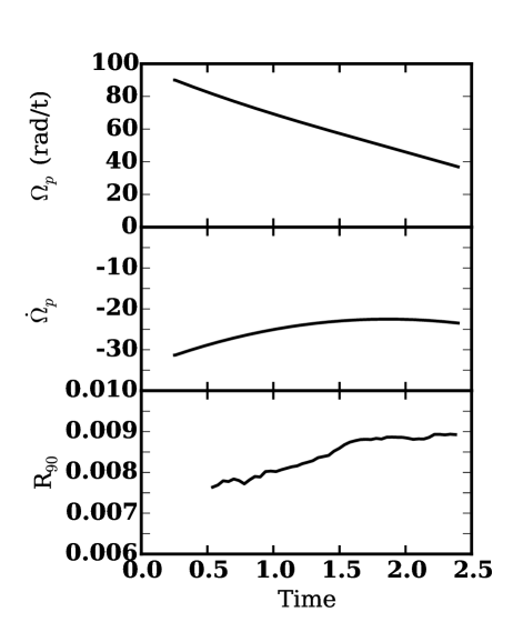
Figure 4: Upper panel: the pattern speed of the stellar bar as a function of time for the fiducial simulation. Middle panel: the rate of change in the pattern speed as a function of time. Bottom panel: the characteristic radius of the bar that encloses 90 per cent of the trapped stellar orbits ($R_{90}$) determined by $k$-means analysis. The bar slows nearly linearly at all times while the bar lengthens. Radius and time are given in virial units.

3.2 Orbit taxonomy

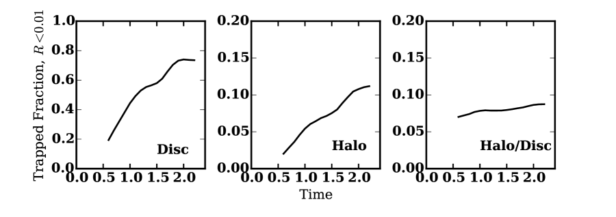
Figure 5: Trapped populations by fraction of mass interior to $R=0.01$ (the initial scale length), as determined by $k$-means power, for the fiducial simulation. Left panel: disc trapping as a function of time. Middle panel: halo trapping as a function of time. The trapped halo fraction (the shadow bar) monotonically increases at all times. Right panel: The ratio of the shadow bar to stellar bar (by total mass) as a function of time. The halo is trapping at a faster rate than the disc, owing to the consistent increase in the reservoir of untrapped matter as the halo contracts in response to the bar growth. Time is given in virial units.

Orbits mediate the transfer of angular momentum between large-scale components (e.g. the disc and halo). For systems dominated by regular orbits for which the derivatives of the potential can be computed exactly (i.e. separable and regular systems), Fourier transformations of particle coordinates can determine the orthogonal frequencies of orbits in cylindrical coordinates ($\Omega_{r},~{}\Omega_{\phi},~{}\Omega_{z}$) and these frequencies allow for rapid and unambiguous determination of orbits trapped into potential features. The most obvious of these features are resonances, commensurabilities of frequencies with the pattern speed of the bar that satisfy the relation

$$l_{r}\Omega_{r}+l_{\phi}\Omega_{\phi}=m\Omega_{p}.$$ (11)

Previous studies have analysed N-body simulations by fixing or ‘freezing’ the gravitational potential after a period of self-consistent evolution and characterise the time-independent orbital structure (e.g. Binney & Spergel 1982, Martinez-Valpuesta et al. 2006, Saha et al. 2012). If the rate of bar evolution is sufficiently small compared to the time required to cross the resonance zone ($\dot{\Omega}_{p}=\mathcal{O}(\epsilon)$ and $\dot{I}_{\rm bar}=\mathcal{O}(\epsilon)$ as $\epsilon\rightarrow 0$, where $\dot{I}_{\rm bar}$ is the time derivative of the moment of inertia of the bar), the dynamics will be approximately described by secular theory (e.g. Tremaine & Weinberg 1984, Weinberg 1985, Hernquist & Weinberg 1992). However, realistic potentials are continuously evolving, so one must attempt a finite-time analysis of secular processes to investigate the nonlinear effects. In other words, one must devise techniques that characterise orbits while the bar pattern speed and geometry change. To this end, we have developed a $k$-means classifier for orbits, which quickly and accurately decomposes particles into orbital components classified by their commensurabilities. Briefly, the $k$-means technique (Lloyd, 1982) iteratively sorts a collection of points into $k$ clusters given a distance metric. For our application, we use a time series in the $r$ and $\theta$ (azimuthal angle) positions of apsides (radial turning points, $r_{\rm max}$) for a given orbit to determine its membership in the bar. As a first application of the method in this work, we limit our analysis to $k=2$.

In a frame corotating with the bar, the apsides of orbits trapped by the bar do not precess through $2\pi$. That is, the azimuthal position of outer turning points for trapped orbits oscillate about some fixed position angle in the bar frame of reference. We exploit these slowly changing apse positions for trapped orbits to identify coherent bar-supporting orbits over a finite time period. Specifically, we define $\delta\theta_{\parallel}$ to be the absolute value of the difference in azimuthal angle between the outer turning point of a particular orbit and the bar position angle. Let $\langle\delta\theta_{\parallel}\rangle_{20}$ be the average value of $\delta\theta_{\parallel}$ in $20$ azimuthal periods for a given orbit. We use the $k$-means technique to identify orbits with $\langle\delta\theta_{\parallel}\rangle_{20}<\pi/8$. Orbits that are periodic and aligned with the bar in its corotating frame have $\langle\delta\theta_{\parallel}\rangle_{20}=0$ while those with no correlation have $\langle\delta\theta_{\parallel}\rangle_{20}=\pi/4$. Additionally, relevant resonances trap orbital apsides perpendicular to the bar. In this case, we define an analogous $\delta\theta_{\perp}$. In practice, this technique allows for rapid determinations of bar membership over time windows that are too brief for frequency determinations using Fourier techniques. In many cases, the bar evolution is so rapid that an analysis in a frozen potential would not be relevant.

After testing a range of period windows, the choice of 20 azimuthal periods was chosen as a balance between minimizing sampling noise while retaining temporal resolution of the evolutionary time scale. Our method is applicable to all but the most extremely centrally confined particles whose azimuthal periods are too small to satisfy an approximate Nyquist criterion. For the simulations here, this critical azimuthal period is $T_{\theta}=0.004$ and affects approximately 0.1 per cent of the orbits. As a simple verification test, we analysed the fixed disc potential simulation (i.e. non-axisymmetric disc evolution is disallowed, Ff in Table 1), finding a bar signal of $<$0.1 per cent, demonstrating that the method is very robust against false positives.

For this paper, we will abbreviate our discussion by assuming that all orbits trapped by the bar potential are 2:1 orbits–those that exhibit two radial periods in every azimuthal period, identified by $k=2$. In reality, the primary resonance bifurcates into 4:1 and 2:1 orbits at high bar strength near the ends of the bar (Athanassoula, 1992). An in-depth discussion of the $k$-means identifier and its application to orbital family determination will be presented in a later paper.

3.2.1 Disc orbits

Since our understanding of secular evolution is informed by perturbation theory, we describe the orbital behaviour in the disc by conserved quantities; here we choose energy and the in-plane angular momentum, $E$ and $L_{z}$. At radii larger than the corotation radius (hereafter, CR), orbits have low ellipticity ($e<0.1$). Inside of CR, the ellipticity increases owing to the bar. The bar-parenting orbit family (${\bf x}_{1}$ in the notation of Contopoulos & Papayannopoulos 1980) is an orbit family whose outer turning points align. These arise from the inner Lindblad resonance (ILR) in perturbation theory. Such orbits are easily identified with the $k$-means identifier.

As a first application of the $k$-means method, we identify the radius that encloses 90 per cent of the bar-trapped disc orbits as the characteristic bar radius, $R_{90}$. The bottom panel of Figure 4 shows that the radius of trapped orbits increases monotonically with time, corroborating previous works indicating the lengthening of bars over time. The trapped fraction of disc orbits satisfying $R<0.01$ is an explicit measure of the bar mass and, therefore, the bar potential (see the left-hand panel of Figure 5). The fiducial simulation exhibits a monotonic increase in the trapped fraction with time. Further, the growth of the bar can be roughly divided into three phases: formation, fast growth, and slow growth. The first, formation ($T<0.5$ in Figure 5), is not studied in this work. We instead begin our study of orbits at times after which the bar can be detected through ellipse fitting, the fast growth phase. In this phase ($0.5<T<1.2$), the bar rapidly gains mass and significant $m=2,4,6$ patterns are observed beyond $R_{d}$. In the third phase ($T>1.2$), the bar continues to add mass (albeit at a diminished rate), but the disc is relatively devoid of other $m\neq 2$ features.

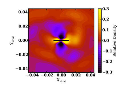
Figure 6: The halo wake ($(m>0)+(m=0,n\neq 0)$, filled colour) with the bar position and length indicated as the thick black line. The wake lags behind the bar (rotating clockwise) at $R>0.5R_{d}$, but is generally aligned with the bar within $0.5R_{d}$, where we observe significant trapping (see Fig. 5). Note the resemblance to the untrapped component of the disc in Fig. 3. Positions are given in virial units, as in Fig. 3.

3.2.2 Halo orbits

The structure of the dark matter distribution in the stellar disc has recently been debated, with particular discussion regarding the creation of a co-rotating ‘dark disc’ (Read et al., 2008; Bruch et al., 2009; Read et al., 2009; Purcell et al., 2009; Pillepich et al., 2014). This dark disc is formed by the accretion of satellites that settle into a rotating structure through dynamical friction, affecting the local dark matter density by contributing up to 60 per cent in some simulations (Ling, 2010), but very little in others (Pillepich et al., 2014). Additionally, the halo is shown to be prolate at small radii in the presence of a stellar bar, referred to as the ‘halo bar’ or ‘dark matter bar’ (Colín et al., 2006; Athanassoula, 2007; Athanassoula et al., 2013; Saha & Naab, 2013), though Debattista et al. (2008) demonstrated that if the disc were evaporated, the prolate inner region of the halo would recover its initially spherical shape.

In our fiducial simulation, the dark-matter halo becomes oblate near the disc at late times. We also refer to this as the ‘dark disc’, while noting the difference in formation mechanism from previous authors. This dark disc is a necessary consequence of the gravitational potential of the disc instead of depending on accretion. We, therefore, expect this dark matter feature to be a generic consequence of stellar discs. At $T=2.0$, long after the bar has formed, and at $R=0.03$, approximately the radius where the disc and halo contributions to the rotation curves are equal, a determination of the ellipsoidal shape of the halo following the method of Allgood et al. (2006) finds $S\equiv c/a=0.45$ (as well as $Q\equiv b/a=0.8$), where $a$, $b$, and $c$ are the lengths of the major, intermediate, and minor axes, respectively. While some of this flattening is attributable to adiabatic compression of the halo in response to the presence of the stellar disc, a test simulation that allows the halo to achieve equilibrium while holding the initial disc potential fixed demonstrates that adiabatic compression alone, which gives $S=0.6$ and $Q>0.99$, cannot account for their deviation from the initially spherical distribution. In the plane of the disc, the effect is even more pronounced; at $R=0.03$ for all $T>1.0$, the azimuthal average of the density in the disc plane is $>$30 per cent larger than the initially spherical distribution.

Examining the evolution of the halo flattening in the fiducial simulation reveals that the initial response of the halo to the presence of the disc is complete by $T=0.3$, in the midst of bar formation; at $T=0.3$ and $R=0.03$ in the fully self-consistent simulation we find that $S=0.6$ and $Q=0.95$. The similarity of these values to that of the settled halo in the fixed disc potential test at late times suggests that the evolution of the disc is responsible for the continued compression and the move to triaxiality. Furthermore, the continued evolution of the halo shape suggests that simply including adiabatic compression in halo models is insufficient to recover the dynamics of the stellar disc and halo.

The distribution of $\cos\beta\equiv L_{z}/L$ also illuminates the flattening of the halo. A perfectly spherical halo will exhibit uniform coverage in $\cos\beta$ owing to the random orientations of the orbital planes. However, at high binding energy (small radii), where the disc dominates the potential, the halo shows enhanced populations at $\cos\beta\approx 1$. Taken together, the continued flattening of the halo and the distribution of $\cos\beta$ suggest that the continued deposition of angular momentum into the halo owing to secular torques from the bar causes the formation of the dark disc in our simulations.

Clearly, the perturbative effect of the stellar bar on the halo cannot be ignored. To investigate the secular response of the halo orbits to the bar, we apply the $k$-means analysis to these orbits as well and find a class of 2:1 orbits that respond similarly to the bar as their disc analogues. In other words, the presence of the stellar disc traps initially spherical halo orbits into not only planar orbits, but into bar-supporting orbits that we call the shadow bar. We emphasise that this result is qualitatively different from those of Debattista et al. (2008), whose orbits are necessarily untrapped if they retain their box-like nature relative to the triaxial halo upon evaporation of the disc. We cannot comment on the likelihood of a similar box orbit-retaining outcome for other studies that point out a bar-like feature in the halo (Colín et al., 2006; Athanassoula, 2007; Athanassoula et al., 2013).

The growth rate of trapped halo orbits also follows that of the stellar bar, albeit with a smaller fraction of the halo mass available for trapping at $R<0.01$ (the middle panel of Figure 5). The continued growth of the trapped fraction during the simulation corroborates that halo trapping is secular and not merely a result of the initial settling of the halo in response to the stellar disc. In the rightmost panel of Figure 5, we plot the ratio of dark matter trapped mass to stellar trapped mass (the total for the simulation rather than that scaled to the mass interior to $R_{d}$). This also rises monotonically throughout the simulation, owing to both the presence of a larger reservoir of planar material as the dark disc grows with time and the increasing strength of the bar potential with time. The result is that the shadow bar grows at a faster rate than the stellar bar.

Overall, the trapped halo orbits exhibit the same behaviour as their trapped disc counterparts: bar-supporting orbits are found at larger radii through time. The trapped orbits in the halo are 5-10 per cent of the trapped mass of disc orbits, and 3-5 per cent of the total trapped angular momentum. That is, the shadow bar is not a large contributor to the mass of the visible stellar bar. However, the existence of shadow bar modifies the rate and location of angular momentum exchange between the bar and halo. Simple perturbation theory calculations following the model presented in Weinberg (1985) demonstrate that the halo orbits that accept $L_{z}$ from the disc are preferentially located near $\cos\beta=1$ and these orbits are the ones that are efficiently trapped into the shadow bar. If we bin the halo orbits by $\cos\beta$, we find that at $T=2.0$, approximately 45 per cent of the orbits satisfying $\cos\beta>0.9$ in the annulus $0.003<R<0.01$ are trapped, compared to 12 per cent for all dark matter at $R<0.01$ (see Figure 5). Preferential trapping of orbits with $\cos\beta>0.9$ suggests that the shadow bar will decrease the angular momentum transport from the bar to the halo relative to that predicted by dynamical friction theory. We will estimate the magnitude of these effects in section 3.4. In the case of a dark disc formed through satellite accretion, whose distribution would be concentrated near $\cos\beta=1$ rather than evenly distributed in $\cos\beta$, we would expect to observe enhanced trapping relative to what is presented here.

Moreover, the overall contribution of the dark matter wake has a very long reach. To see additional effects of the shadow bar on the halo at large scales, we plot the in-plane wake (as in Weinberg & Katz 2007a) at $T=2.0$ in Figure 6. Here, we define the halo wake as the response of the untrapped halo to the non-axisymmetric bar. We find the halo wake by removing all the trapped orbits as found by the $k$-means analysis and comparing the resulting distribution to the lowest order axisymmetric density profile. To accomplish this, we constructed a new basis using only the untrapped orbits (as described in section 2.2) and then removed the lowest order ($m=0,~{}n=0$) component to find the wake. Despite removing the trapped orbits, we observe a strong quadrupole feature that follows the stellar bar (along the $x$-axis) and extends to the end of the stellar bar (the extent of the stellar bar is shown as the black line). Beyond the extent of the bar, an $m=2$ pattern is observed, a direct result of the secular evolution detailed in Weinberg (1985). If the disc scale length of the simulation is scaled to that of the MW, this wake extends out to the Solar circle at approximately the 10 per cent level. This scaling of the simulation may not be the most appropriate due to the apparent disagreement between the bar length-scale length relationship in our simulation and the MW. If the simulation is instead scaled to the bar length of Wegg et al. (2015), 4.6 kpc, the density enhancement from the wake may be as large as 25 per cent!

3.3 Dynamical properties of orbits

To understand the dynamics of the trapped halo orbits, we investigate the distribution of conserved quantities in the various orbit populations. We characterise the orbits by energy $E$, an isolating integral for all regular orbits, and $L_{z}/L_{\rm max}(R)$, where we normalise the angular momentum perpendicular to the disc, $L_{\rm z}$, by the angular momentum of a circular orbit with the same energy, $L_{\rm max}$. Figure 7 shows the distribution of $\langle\delta\theta_{\parallel}\rangle_{20}$ for stellar orbits from the fiducial simulation at $T=2.0$. Orbits with $\langle\delta\theta_{\parallel}\rangle_{20}<\pi/8$ reliably indicate bar-trapped orbits. As expected, the strongest signal comes from mildly elliptical orbits with $L_{z}/L_{\rm max}(R)=0.5$ near the end of the bar with $E=-9.5$ ($R=0.01$). Many of the orbits within a characteristic radius of the bar are trapped (exhibiting $\langle\delta\theta_{\parallel}\rangle_{20}<\pi/8$), though Figure 5 indicates that not all orbits within $R=0.01$ are trapped.

A similar exercise performed for the halo (Fig. 8) reveals that trapped halo orbits occupy the same region in $E-L_{\rm z}$ parameter space as the trapped disc orbits. Because the fiducial halo is initially isotropic the quantity $L_{z}/L_{\rm z,max}(R)$ can have values from -1 to 1. The shadow bar reveals itself by the prominent $\langle\delta\theta_{\parallel}\rangle_{20}<\pi/8$ feature in the upper left corner of Figure 8 at $E<-9$ ($R<0.01$). This reinforces our finding that both dark-matter and stellar orbits are trapped by their mutual gravitational potential, and that the disc and the halo cannot be treated as distinct dynamical components.

In addition to the shadow bar, Figure 8 reveals two planar retrograde families exhibiting $\langle\delta\theta_{\parallel}\rangle_{20}>\pi/3$ (or equivalently $\langle\delta\theta_{\perp}\rangle_{20}<\pi/6$), which correlate with overdensities in Figure 6 and are associated with the ILR and CR resonances. Similarly, we observe the outer Lindblad resonance (OLR, $m=l_{\phi}=2,~{}l_{r}=1$ in the notation of equation 11) as a prograde planar family at $E=-6.5$ ($R=0.04$), observable as an overdense region with $\langle\delta\theta_{\parallel}\rangle_{20}>\pi/3$ in Figure 6. The approximate position of the resonances were located by using the monopole potential field of the disc and halo from the basis so that equation 11 could be solved numerically as a function of $E$ and $\kappa$ when combined with the instantaneous pattern speed of the bar (see Figure 4). We further confirmed the resonant nature of orbits in these $E-\kappa$ regions by examining individual orbits.

To summarise the previous sections, the initially nearly isotropic dark matter halo evolves significantly in the presence of an evolving disc. The effects are three-fold: (1) the trapping of dark matter orbits into the shadow bar; these orbits subsequently behave just like stellar bar orbits; (2) the dark disc, a response to the presence of the stellar disc as well as secular torques from the stellar and shadow bar; these orbits do not resemble the stellar disc per se, but more importantly do not resemble initial halo orbits; and (3) the dark matter wake, created by the influx of $L_{\rm z}$ from the stellar disc.

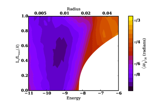
Figure 7: The distribution of $\langle\delta\theta_{\parallel}\rangle_{20}$ as a function of energy, $E$, vs. scaled angular momentum, $L_{\rm z}/L{\rm max}(R)$, at $T=2.0$ for the stellar disc. At each radius, $L_{\rm z}$ and $E$ are calculated for a circular planar orbit and used to determine the mapping between energy and radius, as well as the maximum $L_{\rm z}$ at a given radius. The quantity $L_{\rm z}/L_{\rm max}(R)$ is zero for a radial orbit and unity for a circular orbit. Nearly all disc orbits are prograde, $L_{\rm z}/L_{\rm max}(R)>0$. The colours denote the average apse position relative to the position angle of the bar. The region in $E$-$L_{\rm z}$ space with insufficient density to obtain a reliable estimate is white. The disc is largely comprised of circular orbits at $R>0.02$. The dark blue region indicates the stellar bar. Radius and energy are given in virial units, see Section 2.1.

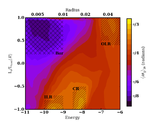
Figure 8: As in Fig. 7 but for the dark matter halo. Retrograde orbits are now present and the $L_{\rm z}/L_{\rm max}(R)$ axis now runs from -1 to 1. The dark blue region in the upper left, with an x-hatched region overlaid, indicates orbits trapped into the shadow bar, which occupies the same region in $E-L_{\rm z}$ space as the stellar bar (compare to Fig. 7). Additional features from the $k$-means analysis are also seen, including two retrograde populations at $E=-9.5$ and $E=-8.2$ that are transiently moving through the ILR and the CR, respectively. A prograde population is observed at OLR, $E=-6.5$. These populations correspond to the wake overdensities in Fig. 6. As in Fig. 7, radius and energy are given in virial units.

3.4 Observational consequences of the shadow bar

Although the trapped dark-matter mass fraction is small, even a small change in $L_{z}$ for halo 2:1 orbits affects both the structure of the dark matter halo and the evolution of the stellar disc in our simulations, and these dynamics are reflected in observable properties of each. In this subsection, we discuss the global implications of several facets of the dark-matter halo response, focusing first on changes to the density and velocity structure, effects that might be traced by halo stars (e.g. observable by Gaia), and then turn to implications for the fast bar–slow bar formation scenarios.

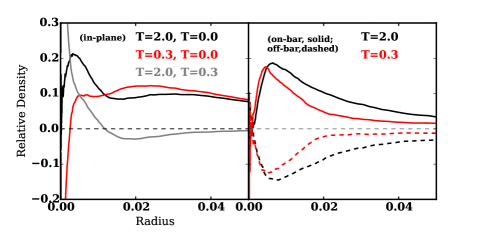
Figure 9: Left panel: the in-plane dark matter density ratio for axisymmetric density profiles at three pairs of times. The black line compares $T=2.0$ with $T=0.0$ (the total change in the profile during the simulation), the red line compares $T=0.3$ to $T=0.0$ (the change in the halo distribution induced by bar formation), and the grey line compares $T=2.0$ to $T=0.3$ (changes caused by secular evolution). The halo has dramatically redistributed its density in response to the presence of a stellar disc by $T=0.3$, but continues to evolve secularly owing to the presence of the bar. Outside of $R=0.05$, the fractional density difference rapidly falls to zero. Right panel: the in-plane fractional dark matter density ratio parallel to the bar and perpendicular to the bar, compared to the axisymmetrised profile, for two times. The on-bar radial cut shows an enhancement at a $>$5 per cent level within $R=0.02$ following bar formation ($T=0.3$), and a $>10$ per cent enhancement within $R=0.02$ after further evolution ($T=2.0$). Radius and time are given in virial units, as in Fig. 2.

3.4.1 Density and velocity structure

The bar changes the density and velocity structure of the dark matter halo. The dark disc in the fiducial simulation appears as an in-plane overdensity that grows with time. However, the non-axisymmetric structure of the shadow bar also contributes to density variations in the plane. Figure 9 demonstrates these two effects at play. In the left panel, we plot the axisymmetric density (azimuthally averaged) ratios for three pairs of times to directly explore the temporal evolution of the planar density without the shadow bar. Over the course of the entire simulation, from $T=0$ to $T=2$ ($\delta T=4$ Gyr scaled to the MW; black curve), the in-plane density out to $R=0.05$ (15 kpc for the MW) increases everywhere by $>8$ per cent . Inside of $R=0.01$, the density increases by up to 20 per cent. For comparison, the evolution from $T=0$ to $T=0.3$ is shown in red, demonstrating that the majority of the azimuthally averaged evolution at $R>0.015$ (4.5 kpc for the MW) happens as the bar is forming. The evolution from $T=0.3$ to $T=2$ ($\delta T=3.4$ Gyr for the MW), shown in grey, corroborates this, and shows that the in-plane density at $R<0.015$ increases dramatically as the bar continues to grow.

The right-hand panel of Figure 9 examines the density on and off the bar axis, relative to the axisymmetric density, at two different times. The dark matter distribution is significantly non-axisymmetric at $T=0.3$, in the midst of bar formation, including an enhancement of up to 17 per cent at $R=0.005$ (1.5 kpc for the MW). At $T=2.0$, the asymmetry is more pronounced enhancing the overdensity in the direction of the bar to 10 per cent out to $R=0.02$ (6 kpc for the MW) and to 5 per cent out to $R=0.035$ (10.5 kpc for the MW), as well as shifting the peak overdensity to a larger radius as compared to $T=0.3$. Although the azimuthally averaged profile remains roughly unchanged at $R>0.015$, the bar produces significant non-axisymmetric halo evolution at all relevant disc radii.

Further, the isotropic nature of the dark matter halo velocity in the plane of the disc has been significantly altered through an infusion of $L_{\rm z}$ from the disc. In the left panel of Figure 10, we plot the tangential velocity distributions on- and off-bar for particles (black and red curves, respectively) near the end of the bar ($0.008<R<0.01$) at $T=2$. For comparison, the dashed black line indicates a normal distribution with the same tangential velocity dispersion, centred at zero velocity. Along the bar axis, the peak of the tangential velocity ($V_{\theta}$) distribution is shifted by $\delta V_{\theta}=0.2$ (30$~{}{\rm km~{}s^{-1}}$ for the MW). Even off the bar axis, the peak of the tangential velocity distribution has been shifted by $\delta V_{\theta}=0.1~{}$ (15$~{}{\rm km~{}s^{-1}}$ for the MW). Additionally, the tails of both the on- and off-bar distributions are enhanced relative to a normal distribution owing to secular processes reshaping the halo.

In the right panel of Figure 10 we again plot the tangential velocity distribution for the on- and off-bar populations, but now compare it to the disc. We plot the on-bar disc distribution in the same annulus near the end of the bar as the solid grey line and the axisymmetric velocity distribution of velocities in the disc as the dashed grey line. The on-bar disc particles are shifted to higher tangential velocities ($V_{\theta,{\rm bar}}=0.8=120~{}{\rm km~{}s^{-1}}$ for the MW, including a shift between peaks of $\delta V_{\theta}=0.5=75~{}{\rm km~{}s^{-1}}$ for the MW), which the halo reflects, albeit at a smaller $\delta V$ (as discussed above). The on-bar disc distribution also shows an enhancement relative to the axisymmetric distribution at $V_{\theta}=1.4$ that is mildly reflected in the halo. The particles trapped into the bar potential librate around the pattern speed as the flattening and trapping of dark matter particles correlate the velocities to create a non-zero mean velocity distribution that is particularly enhanced along the bar axis (in addition to the generic rotation seen in the off-bar population). In other words, the the $L_{z}$ distribution has been modified, with the enhancement most clearly seen along the bar major axis. We make predictions for the net effect of the above considerations on dark matter direct detection experiments in Petersen et al. (2016).

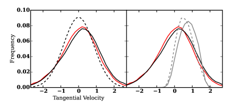
Figure 10: Left panel: Tangential velocity distributions at $T=2.0$ on- (solid black) and off-bar (red) for the dark matter halo, at $R=0.008$ (near the end of the bar). The dashed black line indicates a normal distribution. The tangential velocity distribution on the bar axis (solid black) shows both an enhancement centred near $V_{c}=0.8(120~{}{\rm km~{}s^{-1}}$ for the MW $)$, approximately the bar velocity at this radius, as well as a shift in the overall velocity peak. Both curves show enhanced tails relative to the normal distribution, at velocities $V_{c}<-1.5$. Right panel: The same dark halo tangential velocity distributions as the left panel are plotted, along with the disc on-bar distribution and axisymmetric distribution shown as the solid grey and dashed grey lines, respectively (scaled by 0.6). Tangential velocity is given in virial units, as in Fig. 1.

Although our fiducial model is motivated by $\Lambda$CDM simulations (halo) and direct observations (disc), it represents a single realisation from a particular model family. We emphasise that these observational conclusions are likely to vary even within a model family. However, we expect that the dynamical nature of the density and velocity differences driven by the shadow bar will be generic. To reduce the uncertainty of these simulation-derived quantities for application to Earth-based dark matter detection experiments, at least three additional pieces of information are critical. First, both the density and velocity signatures will be affected by the assumed length of the MW bar and its evolution as a function of time. Relative to the disc scale length, our bar is shorter than the observed MW bar (Wegg et al., 2015); also, the MW bar may have been longer in the past depending on its formation mechanism. Therefore, dark matter at the solar radius maybe have been influenced more readily. Secondly, we have demonstrated that the velocity structure depends on the position angle of the bar, so we need an accurate determination of the MW bar position angle. Finally, we need the formation time of the MW bar. The shadow bar continues to grow in time relative to the mass of the stellar bar. Therefore, an older MW bar would have more trapped dark matter material relative to the stellar bar. An older MW bar may also have a different velocity structure due to trapped dark matter orbits contributing to the torque on the untrapped halo component and the efficiency of $L_{z}$ transfer from the enhanced mass of the shadow bar.

3.4.2 Angular momentum transport

The shadow bar contains a large fraction of the dark-matter orbits at low inclination: $>45$ per cent of dark matter orbits satisfying $0.003<R<0.01$ and $0.9<\cos\beta\leq 1$ are trapped, as discussed in section 3.2.2. The low inclination orbits are the same orbits responsible for accepting angular momentum and slowing the bar as determined by examining the model of Weinberg (1985). We expected that this would diminish the torque relative to the canonical perturbation theory results (e.g. Tremaine & Weinberg 1984). We test this speculation by azimuthally shuffling the halo orbits as described in section 2.1.3. The purpose of this simulation is to prevent the shadow bar from forming and mimic the standard dark-matter halo dynamical friction scenario. Figure 11 compares the results of the fiducial simulation to the azimuthally shuffled experiment. The azimuthally-shuffled halo is able to transfer angular momentum continuously, evident through the rapidly decreasing pattern speed during the evolution. Given the assumption that $\Delta L\approx\Delta\Omega_{p}$ for a stellar bar with the same geometry, we find that $\Delta\Omega_{p,{\rm shuffled}}/\Delta\Omega_{p,{\rm self-consistent}}\approx 3$, an appreciable increase in torque. Clearly, inhibiting the formation of the shadow bar results in a strong torque on the bar by the halo. We only present the results of the simulation for $T<1.2$ because after this time the resultant stellar bars no longer qualitatively resemble each other ($I_{\rm bar,shuffled}\neq I_{\rm bar,self-consistent}$ where $I$ is the moment of inertia of the bar), making the comparison of the simulations unfair.

The shadow bar does not eliminate the torque altogether, of course. A massive bar, enhanced by the dark matter, will couple more strongly to higher order resonances, even though these resonances are much weaker. The relative strength can be roughly approximated by considering the inverse of the largest winding number in the resonant equation (the maximum of $[m,~{}l_{\phi},~{}l_{r}]$ in equation 11) for a particular resonance. For example, the 4:2:1 resonance will be approximately half as strong as the 2:2:1 resonance, and so on, for all realistic distribution functions (Binney & Tremaine, 2008). However, the primary (low-order) resonances are weakened by the reduction in available dark matter to accept angular momentum as more halo material becomes trapped. An enhanced dark disc, fed through satellite accretion, could act as a larger reservoir for material to trap, with presently unexplored implications for the torque.

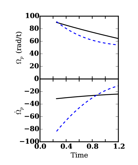
Figure 11: Upper panel: the pattern speed for the fiducial simulation (black) and an azimuthally-shuffled halo to suppress shadow bar formation (Fs; the dashed blue line). The simulation time is limited to $T<1.2$ so that the stellar bars that form are still roughly equivalent. Lower panel: Change in pattern speed, following the same colour scheme. The shuffled simulation slows much more rapidly during the simulation, indicative of an increased $L_{\rm z}$ acceptance by the halo when there is no shadow bar. Time is given in virial units, as in Fig. 4.

4 Comparison between our fiducial and other models

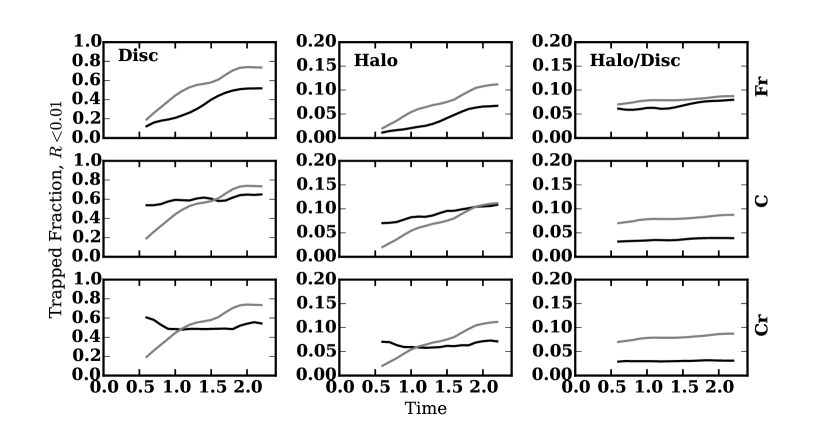
Figure 12: From left to right: stellar disc trapping, dark matter trapping, and the ratio of dark-matter halo to stellar disc trapping by the bar inside $R=0.01$. Compare these to Fig. 5. From top to bottom the simulations are: the cusped rotating halo (Fr in Table 1), the cored nonrotating (C), and the cored rotating (Cr) models. Black lines indicate the total mass trapped scaled by the mass interior to $R=0.01$ and grey lines indicate the corresponding curve for the fiducial model. Time is given in virial units, as in Fig. 5.

4.1 Halo initial conditions

Our fiducial model is a simple representation of a disc galaxy in the $\Lambda$CDM formation scenario: a cuspy dark-matter halo profile with an exponential stellar disc. However, there are a variety of alternatives that are commonly explored in the literature. These include models whose density approaches a constant at some characteristic core radius $r_{c}$ and rotating halo models (models with a non-zero value of $L_{z}$). The former, which have some observational (e.g. rotation curves, Breddels & Helmi 2013) and theoretical motivation (e.g. satellite accretion producing cores, black holes, and feedback from star formation or supernova; Tremaine & Ostriker 1999, Mashchenko et al. 2006, Governato et al. 2012) have often been used in N-body bar simulations (Athanassoula & Misiriotis 2002, Martinez-Valpuesta et al. 2006, Saha et al. 2010). The latter are motivated by both evolutionary processes such as merging (Dekel et al., 2003) and the hierarchical formation process itself (Navarro et al. 1997, Bullock et al. 2001). In this section, we briefly summarise the variation in the properties of the disc and shadow bars for a representative member of each of these two model classes.

Table 1 describes the halo models we tested in addition to the fiducial cuspy non-rotating model. The resultant disc and shadow bar evolutions are shown in Figure 12, the analogue of Figure 5. The qualitative evolution is similar between all four simulations, suggesting that the results presented in section 3 are generally relevant. In particular, the shadow bar continues to grow relative to the stellar bar in all the simulations (the right panel of Figure 12). The fiducial model exhibits the strongest stellar and shadow bars at late times as a fraction of the available mass, but the trend in each model suggests that an equilibrium has not been reached at $T=2.0$, the end of the simulations. (Recall that one system time unit is approximately 2 Gyr scaled to the MW, so that $T=2.0$ is roughly 4 Gyr or 40 per cent of the age of the Galaxy.) The cored halo models exhibit a buckling instability at $T=0.6$ in the cored nonrotating model, and at $T=1.0$ in the cored rotating model. This instability releases disc orbits trapped during the bar formation phase, albeit a relatively small fraction, and does not appear to reduce the dark-matter fraction relative to the trapped disc fraction.

Overall, the differences in evolution between the models can be described as follows: (1) the cored halo increases the initial strength of the stellar bar through a stronger instability (rapid growth at $T<0.6$). However, the relative strength of the shadow bar is smaller and stagnant at late times owing to the reduced central density and, consequently, a smaller population of halo orbits that are available to trap; and (2) the increased rotation of a halo affects models by reducing the strength of the bar at early times (diminished the growth between $T=0.5$ and $T=1.0$); the stellar and shadow bars take longer to dynamically mature and, consequently, have not evolved to be as massive over the same span of time. This effect is smaller in the cored rotating halo compared to the cusped rotating halo, suggesting that the cuspy or cored nature of the halo dominates the evolution when compared to rotation in these models. We will discuss these trends further in a future paper.

4.2 Disc Maximality

As discussed in section 2.1.1, our fiducial model is a submaximal disc (as are all F-series models), chosen to correspond to cosmological simulations. Simulations with maximal discs (such as the C-series models) are subject to a violent disc instability that results in a qualitatively different bar formation scenario than that of our fiducial F-series models. The violent disc instability may create a noisy bar formation process that inhibits the formation of the dark disc required for the stellar bar to then trap into the shadow bar. The C-series models nearly reach their maximum trapping fraction within several dynamical times of formation where the F-series models trap continuously over many dynamical times (see Figure 12). This illustrates a the distinct differences between the fast and slow mode of bar growth in our models. The variations with time, including untrapping of some orbits, suggest that the trapping is more tenuous in a violent instability. The fast and slow modes of bar growth will be studied further in future work. If these differences can be detected in an out-of-plane luminous tracer population (e.g. spheroid or thick disc stars in the Milky Way), we may be able to discriminate between these two modes of formation in nature.

It is also likely that the relative contributions to the potential from the disc and halo will change the formation efficiency of the shadow bar, an effect we have already seen qualitatively in the contrast between the cusp and core simulations. In the simulations with cores, the halo material interior to $R_{d}$ is approximately half that in the cusp simulation, so that even when the same fraction of material is trapped (e.g. the middle panel of the cored simulation in Figure 12), the contribution to the overall bar potential is low (e.g. the right panel of the cored simulation in Figure 12). Furthermore, a more violent formation of the bar may change the structure of the dark matter wake. In this bar formation scenario, the formation of the dark disc and subsequent shadow bar trapping, both of which are slow processes, could be disrupted. A study of the implications of stellar disc maximality for the shadow bar and dark matter wake will be investigated in future work.

5 Conclusion

Our main findings are as follows:

1. The stellar bar traps dark matter into a shadow bar. This shadow bar has a mass that is $>$6 per cent of the stellar bar mass after the bar forms, and this ratio increases with time throughout the simulations to values $>$9 per cent by mass. The halo is deformed by the presence of the disc as well as the continued torque from the stellar and shadow bar, creating a population of disc-like orbits (with a preferred angular momentum axis). We suggest that this reservoir increases the trapping rate of dark matter orbits.

2. Trapping in the dark matter halo and the stellar disc takes place both at bar formation and throughout the simulation.

3. The existence and strength of the shadow bar does not change appreciably in the presence of a core or rotation in the halo. However, the trapping rate of both the dark matter halo and the stellar component strongly depends on halo profile and the initial angular momentum distribution in the halo.

4. The dark matter halo exhibits a density and velocity signature indicative of a reaction to the presence of the stellar disc at radii much larger than that of the bar radius. The density and velocity structure change with the angle to the bar, even at several bar radii. This could have important implications for direct dark matter detection experiments.

5. Approximately 12 per cent of the total halo inside of the bar radius ($R<0.01$), and 45 per cent of the dark matter satisfying $\cos\beta>0.9$ within $0.003<R<0.01$, is trapped after 4 Gyr. These trapped orbits are precisely the ones that dominate the secular angular momentum transfer to the halo in the absence of trapping. The trapping changes the secular angular momentum transfer rates that one would estimate without trapping. We demonstrate this point with a simulation that suppresses trapped orbits by artificially decorrelating the halo orbit apsides with the bar position. This increases the halo torque on the bar after formation by a factor of three! Stronger bars are likely proportionally larger fractions of their haloes. This suggests that halo torques may be much smaller than theoretically predicted, especially for strong bars, helping to resolve the tension between the $\Lambda$CDM scenario and the observational evidence for rapidly rotation bars.

In concept, the idea of trapped dark matter is striking in its simplicity: when disc orbits and halo orbits occupy similar places in phase space, they will respond similarly to a perturbation. We have only begun to explore the parameter space necessary to characterise dark matter trapping, as well as the implications for the evolution of isolated galaxies. Therefore, we expect that other simulations have shadow bars as well, but previous studies have not investigated or identified the halo trapping and have not undertaken a detailed study of trapped populations in the disc component. Our $k$-means orbit finding algorithm can be used as a technique to further understand the dynamics of strongly time-dependent evolution, such as the bar-disc-halo system. In future papers, we will present a detailed breakdown of the orbit populations in the disc and halo components using the $k$-means technique.

Many simulations have shown that galactic bars efficiently transport angular momentum from the disc to the halo, causing the bar to slow, lengthen, and increase in strength (Debattista & Sellwood 2000; Athanassoula & Misiriotis 2002; Debattista et al. 2006; Weinberg & Katz 2007b). Many of these same authors have argued that bars are long-lived, as no mechanism for their destruction has been observed in simulations of isolated systems (e.g. Athanassoula et al. 2013). The results of Hernquist & Weinberg (1992) then suggest that the bar either cannot be strongly coupled to the halo, or requires fine-tuning to eliminate lower-order resonances to reduce the strong torque. The suggestion that bars cannot be strongly coupled to the halo seems to be in direct conflict with the angular momentum transfer rates observed in simulations depicting a rapidly slowing bar. The production of a shadow bar, and the trapping of halo orbits by the bar more generally, offers a possible way out of this dynamical conundrum. Without a sink of halo particles that are distributed asymmetrically in phase space relative to the bar, there can be no torque. Our discussion in section 4.1 suggests that the existence of the shadow bar is robust, but that its magnitude will depend on the galaxy profile and the details of the subsequent bar formation. If a significant dark disc exists as the remnant of shredded satellites accreted by the galaxy, the magnitude of the shadow bar could be significantly enhanced.

Although the shadow bar is kinematically similar to the stellar bar, the findings presented here provide new insight into the kinematics of the galactic centre. Observationally, stellar surveys may detect rotation in the stellar halo toward the inner Galaxy that would be indicative of trapping in a spherical component. For stars and stellar systems that may have formed prior to the formation of the MW bar (such as metal-poor halo stars, thick-disc stars, or globular clusters), the findings presented here indicate that these components could also be trapped into the bar potential. Suggestions in the literature dating as early as Blitz & Spergel (1991) of a triaxial rotating component at the centre of the galaxy could be the result of an originally spheroidal component trapped by the bar potential. Recent observations by Babusiaux et al. (2014) and Rossi et al. (2015) have pointed out kinematic signatures (e.g. an anomalous tangential and radial velocity dispersion) that could be consistent with this interpretation. New stellar survey data available in the coming years will provide further insights. The results of this paper suggest that stellar survey data may be able to discriminate between fast and slow-growth bar formation and evolution in the MW.

Finally, evidence for a shadow bar in our own Milky Way could be directly detected through future direct dark matter detection experiments, including directional direct detection experiments, which would provide significant dynamical insights into the unseen dark matter component.

References

- Aalseth et al. (2013) Aalseth C. E., et al., 2013, PhysRevD, 88, 012002
- Agnese et al. (2013) Agnese R., et al., 2013, PhysRevD, 88, 031104
- Aguerri et al. (2015) Aguerri J. A. L., et al., 2015, A&A, 576, A102
- Allende Prieto et al. (2008) Allende Prieto C., et al., 2008, Astronomische Nachrichten, 329, 1018
- Allgood et al. (2006) Allgood B., Flores R. A., Primack J. R., Kravtsov A. V., Wechsler R. H., Faltenbacher A., Bullock J. S., 2006, MNRAS, 367, 1781
- Athanassoula (1992) Athanassoula E., 1992, MNRAS, 259, 328
- Athanassoula (2007) Athanassoula E., 2007, MNRAS, 377, 1569
- Athanassoula & Misiriotis (2002) Athanassoula E., Misiriotis A., 2002, MNRAS, 330, 35
- Athanassoula et al. (2013) Athanassoula E., Machado R. E. G., Rodionov S. A., 2013, MNRAS, 429, 1949
- Babusiaux et al. (2014) Babusiaux C., et al., 2014, A&A, 563, A15
- Barnes et al. (1986) Barnes J., Hut P., Goodman J., 1986, ApJ, 300, 112
- Bernabei et al. (2014) Bernabei R., et al., 2014, Nuclear Instruments and Methods in Physics Research A, 742, 177
- Binney & Spergel (1982) Binney J., Spergel D., 1982, ApJ, 252, 308
- Binney & Tremaine (2008) Binney J., Tremaine S., 2008, Galactic Dynamics: Second Edition. Princeton University Press
- Blitz & Spergel (1991) Blitz L., Spergel D. N., 1991, ApJ, 379, 631
- Bournaud & Combes (2002) Bournaud F., Combes F., 2002, A&A, 392, 83
- Bournaud et al. (2005) Bournaud F., Combes F., Semelin B., 2005, MNRAS, 364, L18
- Bovy & Rix (2013) Bovy J., Rix H.-W., 2013, ApJ, 779, 115
- Boylan-Kolchin et al. (2013) Boylan-Kolchin M., Bullock J. S., Sohn S. T., Besla G., van der Marel R. P., 2013, ApJ, 768, 140
- Breddels & Helmi (2013) Breddels M. A., Helmi A., 2013, A&A, 558, A35
- Bruch et al. (2009) Bruch T., Read J., Baudis L., Lake G., 2009, ApJ, 696, 920
- Bullock et al. (2001) Bullock J., Dekel A., Kolatt T., Kravtsov A., Klypin A., Porcianai C., Primack J., 2001, ApJ, 555, 240
- Cheung et al. (2013) Cheung E., et al., 2013, ApJ, 779, 162
- Clutton-Brock (1973) Clutton-Brock M., 1973, Ap&SS, 23, 55
- Clutton-Brock et al. (1977) Clutton-Brock M., Innanen K. A., Papp K. A., 1977, Ap&SS, 47, 299
- Colín et al. (2006) Colín P., Valenzuela O., Klypin A., 2006, ApJ, 644, 687
- Contopoulos & Papayannopoulos (1980) Contopoulos G., Papayannopoulos T., 1980, A&A, 92, 33
- Debattista & Sellwood (2000) Debattista V. P., Sellwood J. A., 2000, ApJ, 543, 704
- Debattista et al. (2006) Debattista V., Mayer L., Carollo C., Moore B., Wadsley J., Quinn T., 2006, ApJ, 645, 209
- Debattista et al. (2008) Debattista V. P., Moore B., Quinn T., Kazantzidis S., Maas R., Mayer L., Read J., Stadel J., 2008, ApJ, 681, 1076
- Dekel et al. (2003) Dekel A., Devor J., Hetzroni G., 2003, MNRAS, 341, 326
- Earn (1996) Earn D. J. D., 1996, ApJ, 465, 91
- Gilmore et al. (2012) Gilmore G., et al., 2012, The Messenger, 147, 25
- Governato et al. (2012) Governato F., et al., 2012, MNRAS, 422, 1231
- Hernquist & Ostriker (1992) Hernquist L., Ostriker J. P., 1992, ApJ, 386, 375
- Hernquist & Weinberg (1992) Hernquist L., Weinberg M. D., 1992, ApJ, 400, 80
- Holley-Bockelmann et al. (2005) Holley-Bockelmann K., Weinberg M., Katz N., 2005, MNRAS, 363, 991
- Kim et al. (2014) Kim T., et al., 2014, ApJ, 782, 64
- Kormendy & Kennicutt (2004) Kormendy J., Kennicutt Jr. R. C., 2004, ARA&A, 42, 603
- Kravtsov (2013) Kravtsov A. V., 2013, ApJL, 764, L31
- Kuijken & Dubinski (1994) Kuijken K., Dubinski J., 1994, MNRAS, 269, 13
- Laurikainen et al. (2014) Laurikainen E., Salo H., Athanassoula E., Bosma A., Herrera-Endoqui M., 2014, MNRAS, 444, L80
- Ling (2010) Ling F.-S., 2010, PhysRevD, 82, 023534
- Lloyd (1982) Lloyd S., 1982, IEEE Transactions on Information Theory, 28, 2
- Lynden-Bell & Kalnajs (1972) Lynden-Bell D., Kalnajs A. J., 1972, MNRAS, 157, 1
- Martinez-Valpuesta et al. (2006) Martinez-Valpuesta I., Shlosman I., Heller C., 2006, ApJ, 637, 214
- Martinsson et al. (2013) Martinsson T. P. K., Verheijen M. A. W., Westfall K. B., Bershady M. A., Andersen D. R., Swaters R. A., 2013, A&A, 557, A131
- Mashchenko et al. (2006) Mashchenko S., Couchman H. M. P., Wadsley J., 2006, Nature, 442, 539
- Masters et al. (2012) Masters K. L., et al., 2012, MNRAS, 424, 2180
- Moster et al. (2013) Moster B. P., Naab T., White S. D. M., 2013, MNRAS, 428, 3121
- Muñoz-Mateos et al. (2013) Muñoz-Mateos J. C., et al., 2013, ApJ, 771, 59
- Navarro et al. (1997) Navarro J. F., Frenk C. S., White S. D. M., 1997, ApJ, 490, 493
- Petersen et al. (2016) Petersen M., Katz N., Weinberg M., 2016, PhysRevD
- Piffl et al. (2014) Piffl T., et al., 2014, MNRAS, 445, 3133
- Pillepich et al. (2014) Pillepich A., Kuhlen M., Guedes J., Madau P., 2014, ApJ, 784, 161
- Polyachenko & Polyachenko (1996) Polyachenko V., Polyachenko E., 1996, AstL, 22, 302
- Purcell et al. (2009) Purcell C. W., Bullock J. S., Kaplinghat M., 2009, ApJ, 703, 2275
- Read et al. (2008) Read J. I., Lake G., Agertz O., Debattista V. P., 2008, MNRAS, 389, 1041
- Read et al. (2009) Read J. I., Mayer L., Brooks A. M., Governato F., Lake G., 2009, MNRAS, 397, 44
- Rojas-Arriagada et al. (2014) Rojas-Arriagada A., et al., 2014, A&A, 569, A103
- Rossi et al. (2015) Rossi L. J., Ortolani S., Barbuy B., Bica E., Bonfanti A., 2015, MNRAS, 450, 3270
- Saha & Naab (2013) Saha K., Naab T., 2013, MNRAS, 434, 1287
- Saha et al. (2010) Saha K., Tseng Y.-H., Taam R. E., 2010, ApJ, 721, 1878
- Saha et al. (2012) Saha K., Martinez-Valpuesta I., Gerhard O., 2012, MNRAS, 421, 333
- Sellwood (2014) Sellwood J., 2014, RevModPhys, 86, 1
- Sellwood & Debattista (2006) Sellwood J. A., Debattista V. P., 2006, ApJ, 639, 868
- Sellwood & Debattista (2009) Sellwood J. A., Debattista V. P., 2009, MNRAS, 398, 1279
- Sellwood & Wilkinson (1993) Sellwood J. A., Wilkinson A., 1993, Reports on Progress in Physics, 56, 173
- Sheth et al. (2008) Sheth K., et al., 2008, ApJ, 675, 1141
- Soto et al. (2014) Soto M., Zeballos H., Kuijken K., Rich R. M., Kunder A., Astraatmadja T., 2014, A&A, 562, A41
- Steinmetz et al. (2006) Steinmetz M., et al., 2006, AJ, 132, 1645
- Tiret & Combes (2007) Tiret O., Combes F., 2007, A&A, 464, 517
- Tremaine & Ostriker (1999) Tremaine S., Ostriker J. P., 1999, MNRAS, 306, 662
- Tremaine & Weinberg (1984) Tremaine S., Weinberg M., 1984, MNRAS, 209, 729
- Villa-Vargas et al. (2009) Villa-Vargas J., Shlosman I., Heller C., 2009, ApJ, 707, 218
- Villa-Vargas et al. (2010) Villa-Vargas J., Shlosman I., Heller C., 2010, ApJ, 719, 1470
- Vogelsberger et al. (2014) Vogelsberger M., et al., 2014, MNRAS, 444, 1518
- Wegg et al. (2015) Wegg C., Gerhard O., Portail M., 2015, MNRAS, 450, 4050
- Weinberg (1985) Weinberg M. D., 1985, MNRAS, 213, 451
- Weinberg (1991) Weinberg M. D., 1991, ApJ, 368, 66
- Weinberg (1994) Weinberg M. D., 1994, ApJ, 421, 481
- Weinberg (1998) Weinberg M. D., 1998, MNRAS, 297, 101
- Weinberg (1999) Weinberg M., 1999, AJ, 117, 629
- Weinberg & Katz (2002) Weinberg M., Katz N., 2002, ApJ, 580, 627
- Weinberg & Katz (2007a) Weinberg M. D., Katz N., 2007a, MNRAS, 375, 425
- Weinberg & Katz (2007b) Weinberg M. D., Katz N., 2007b, MNRAS, 375, 460
- Williams et al. (2012) Williams M. J., Bureau M., Kuntschner H., 2012, MNRAS, 427, L99
- Zaritsky et al. (2013) Zaritsky D., et al., 2013, ApJ, 772, 135