Mass and Metallicity Requirement in Stellar Models for Galactic Chemical Evolution Applications
Abstract
We used a one-zone chemical evolution model to address the question of how many masses and metallicities are required in grids of massive stellar models in order to ensure reliable galactic chemical evolution predictions. We used a set of yields that includes seven masses between 13 and M⊙, 15 metallicities between 0 and 0.03 in mass fraction, and two different remnant mass prescriptions. We ran several simulations where we sampled subsets of stellar models to explore the impact of different grid resolutions. Stellar yields from low- and intermediate-mass stars and from Type Ia supernovae have been included in our simulations, but with a fixed grid resolution. We compared our results with the stellar abundances observed in the Milky Way for O, Na, Mg, Si, Ca, Ti, and Mn. Our results suggest that the range of metallicity considered is more important than the number of metallicities within that range, which only affects our numerical predictions by about 0.1 dex. We found that our predictions at [Fe/H] are very sensitive to the metallicity range and the mass sampling used for the lowest metallicity included in the set of yields. Variations between results can be as high as 0.8 dex. At higher [Fe/H], we found that the required number of masses depends on the element of interest and on the remnant mass prescription. With a monotonic remnant mass prescription where every model explodes as a core-collapse supernova, the mass resolution induces variations of 0.2 dex on average. But with a remnant mass prescription that includes islands of non-explodability, the mass resolution can cause variations of about 0.2 to 0.7 dex depending on the choice of the lower limit of the metallicity range. With such a remnant mass prescription, explosive or non-explosive models can be missed if not enough masses are selected, resulting in over- or under-estimations of the mass ejected by massive stars.
keywords:
Galaxy: chemical evolution – Stars: supernovae – Stars: yields1 Introduction
Stellar yields are fundamental ingredients in chemical evolution
models and simulations. To reproduce the chemical enrichment of
galaxies over their entire lifetime, those yields need to include
low-mass, intermediate-mass, and massive stars along with a wide range
of metallicities, ideally from zero metallicity up to solar
composition. Several grids of stellar models are available in the
literature with different numbers of masses and metallicities. In
general, for massive stars, those grids either offer a limited number
of masses within a certain range of metallicities
(e.g., Woosley & Weaver 1995; Portinari et al. 1998; Chieffi & Limongi 2004; Kobayashi et al. 2006; Pignatari et al. 2013)
or a large number of masses for one
specific metallicity (e.g., Limongi & Chieffi 2006; Woosley & Heger 2007; Heger & Woosley 2010; Ekström et al. 2012).
In this paper we address the question of how many masses and
metallicities for massive stars are required in a grid of stellar models to ensure
convergence in galactic chemical evolution studies. To do so, we
conduct an experiment with a set of yields which
has seven masses from 13 to 30 M⊙ and 15
metallicities (see Section 2.5), where we sample subsets of stellar
models to create new sets of yields with lower mass and metallicity
resolutions. We then fold those yields into simple stellar
populations (SSPs) and include them in a one-zone chemical evolution
model to quantify the impact of the stellar grid resolution on our
predictions. For now, we do not consider the impact of
massive binary systems which could significantly alter the evolution
and the ejecta of massive stars (e.g., De Donder & Vanbeveren 2004; Sana et al. 2012; de Mink et al. 2013). Although our sensitivity study
only focuses on massive stars, we included the contribution of low-and
intermediate-mass stars and Type Ia supernovae (SNe Ia) in our calculations (see Section 2.5).
It is generally believed that the most massive stars are more likely
to form a black hole and lock away most of the heavy elements
synthesized during their evolution (e.g., Woosley et al. 2002; Heger et al. 2003; Zhang et al. 2008).
This seems to be also supported by the
lack of observed more massive progenitors for common supernovae
(e.g., Smartt 2009; Williams et al. 2014). This sustains the idea that there must be a
transition mass above which massive stars stop to contribute to the
chemical evolution of galaxies (but see discussion in Section 2.5).
Recent studies with high mass resolutions,
however, suggest that such a transition may not exist and that black
hole formation is in fact sparsely distributed across the stellar
initial mass spectra, forming islands of non-explodability
(e.g., Ugliano et al. 2012; Ertl et al. 2015; Sukhbold et al. 2015).
The yields used in this work for massive stars have been
calculated with four different remnant mass and black hole formation
prescriptions, which enables us to study the impact of such
prescriptions on our grid resolution study. As two extreme cases, we
consider the prescription of Ertl et al. (2015) that generates islands of
non-explodability, and the no-cutoff prescription, which is a
monotonic remnant mass distribution where all models explode with
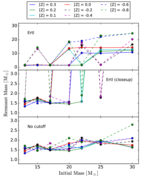
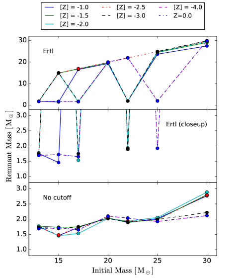
minimum fallback (see Figures 1 and
2). The remnant mass is the baryonic final mass of
a star (i.e., not its gravitational mass) and refers to its initial
mass minus the total mass ejected during its lifetime, which includes
the explosive ejecta, if any, and stellar winds. In our specific
case, any remnant mass larger than M⊙ implies a black
hole formation instead of an explosion. We also assumed that, if a
star does not explode, the entire star disappears as a back hole
and no supernova yield is produced. Whereas this may be a simplification in
some cases, e.g., the formation of long-duration gamma-ray bursts or
some types of hypernovae, it should be reasonable to assume that in
this case the bulk, and in particular the inner parts of the stars,
are not being ejected.
Throughout this paper, we compare our numerical predictions with observations to provide a visual reference to evaluate the importance of the stellar grid resolution in our simulations. We chose the Milky Way because of the large amount of stellar abundances data and because of the wide metallicity range covered by those data. Although one-zone models do not capture the complexity of the formation of massive systems such as the Milky Way, we believe they are sufficient, at least as a first order approximation, to address the specific question of what is the impact of the stellar grid resolution and the remnant mass prescription in the context of galactic chemical evolution. Our results may differ from the ones generated by two-zone and three-zone models (e.g., Ferrini et al 1992; Pardi et al. 1995), since all of our stellar ejecta is returned and recycled in a unique gas reservoir instead of being distributed within the different galactic structures, such as the halo and the thick and thin discs. It is not our goal to produce the most realistic model of the Milky Way. More sophisticated simulations for our Galaxy can be found in the literature (e.g., Chiappini et al. 2001; Travaglio et al. 2004; Kobayashi & Nakasato 2011; Micali et al. 2013; Minchev et al. 2013; Mollá et al. 2015; Shen et al. 2015; van de Voort et al. 2015; Wehmeyer et al. 2015).
This paper is organized as follow. In Section 2, we describe our chemical evolution code and input physics. We describe our stellar abundances data selection in Section 3. The impact of the mass and metallicity resolutions is presented in Section 4 for stellar yields with monotonic remnant masses, and in Section 5 for stellar yields with islands of non-explodability. We summarize our results and give our conclusions in Section 6.
2 Galaxy Model
We use OMEGA, our One-zone Model for the Evolution of GAlaxies code (Côté et al. 2016b), to follow the chemical evolution of the Milky Way. The input parameters of the closed-box version and the treatment of SSPs using SYGMA, which stands for Stellar Yields for Galactic Modeling Applications (C. Ritter et al., in prep.), are described in details in Côté et al. (2016a). For the present study, we consider an open box model that includes and inflows of primordial gas and galactic outflows. All of our codes are available online with the NuGrid NuPyCEE package111https://github.com/NuGrid/NUPYCEE.
2.1 Open Box Model
OMEGA uses the classical equations of single-zone chemical evolution models (Pagel 2009). At a certain time, , the mass of the gas reservoir, , is calculated by
| (1) |
where is the length of the timestep and the four terms in brackets are, from left to right, the inflow rate, the outflow rate, the stellar mass loss rate of all the SSPs, and the star formation rate. The mass ejected by each SSP is calculated using the initial mass function of Chabrier (2003) and the stellar yields described in Section 2.5. We use a star formation history that has a similar shape than the one derived from the two-infall Milky Way model of Chiappini et al. (1997, 2001), which we normalized to produce a current stellar mass of M⊙ (Flynn et al. 2006; McMillan 2011; Bovy & Rix 2013; Licquia & Newman 2015) at the end of our simulations.
2.2 Outflow Rate
The evolution of the galactic outflow rate is defined by (Murray et al. 2005)
| (2) |
To calculate the time evolution of , the mass-loading factor, we use the MA prescription described in Côté et al. (2016b),
| (3) |
where is the total virial mass of the system. The redshift, , is converted into time using the cosmological parameters measured in Dunkley et al. (2009), assuming the end of our simulations represents . We set to unity to consider outflows driven by radiative pressure (see Murray et al. 2005). We assume the dark matter halo mass of the Milky Way follows the equations derived by Fakhouri et al. (2010) which represents the average dark matter accretion rates extracted from the Millennium simulations (Springel et al. 2005; Boylan-Kolchin et al. 2009). In each series of simulations, we tune the final value of the mass-loading factor to ensure that the peak of the predicted metallicity distribution function occurs at [Fe/H] .
2.3 Mass of Gas and Inflow Rate
At every time , we assume the star formation follows the Kennicutt-Schmidt law (Schmidt 1959; Kennicutt 1998) in the adapted form of (Baugh 2006; Somerville & Davé 2015)
| (4) |
where and are respectively the star formation efficiency and the star formation timescale. Because is a known quantity in our code, we can reverse equation (4) and derive the evolution of the mass of gas as a function of time. The inflow rate, the only unknown in equation (1), can then be isolated and calculated for each timestep. This approach has been used in previous works to calculate the chemical evolution of local dwarf spheroidal galaxies (Fenner et al. 2006; Gibson 2007; Homma et al. 2015).
2.4 Star Formation Efficiency and Timescale
We assume that the star formation timescale is proportional to the dynamical timescale, , of the virialized system hosting the galaxy (e.g. Kauffmann et al. 1999; Cole et al. 2000; Springel et al. 2001), and is defined by , where is the proportional constant and and are respectively the virial radius and the circular velocity of the system. With the relation for defined in White & Frenk (1991),
| (5) |
where is the current Hubble constant, the dynamical timescale is then given by
| (6) |
With our set of equations, the ratio is used to control the initial and final mass of gas in our simulations. The initial mass of gas sets the speed and the concentration of the early enrichment and therefore the metallicity at which SNe Ia start to contribute to the chemical evolution, whereas the final mass of gas sets the final metallicity and the fraction of gas converted into stars. We fixed to so that the final mass of gas in our simulated galaxy is M⊙, consistent with the current state of the Milky Way (see Table 1 in Kubryk et al. 2015). This represents a star formation efficiency of 0.04 when . This choice, however, implies a relatively low initial mass of gas and generates a fast early enrichment that pushes the appearance of SNe Ia up to [Fe/H] of , which is too high compared to the canonical value of constrained by observations (see Matteucci & Greggio 1986; Chiappini et al. 2001).
To solve this issue, we introduced a free parameter, , in the exponent of the redshift dependency term of equation (6) so that the star formation timescale is now described by
| (7) |
This assumes that the gas fraction in our galaxy model does not necessarily scale linearly with the dynamical timescale of the virialized system. It allows us to control the growth of the gas content and to tune the initial mass of gas independently of the final mass of gas to make sure that SNe Ia occur at [Fe/H] . The value of depends on the choice of stellar yields and the amount of Fe ejected by massive stars. We recall that our one-zone model is mostly designed to mimic the evolution of known galaxies rather than to study how that evolution is driven. Although the parameter has been introduced for fine-tuning, we believe it is necessary in order to recover the global properties of the Milky Way with our simple model. It allows us to apply our chemical evolution calculations on top of a reasonable gas evolution pattern.
2.5 Stellar Yields
Using the KEPLER stellar evolution, nucleosynthesis, and supernova code (Weaver et al. 1978; Rauscher et al. 2002), we computed a set of non-rotating stellar models and their nucleosynthesis yields with seven different initial masses (see Table LABEL:tab_sample) and for 15 different metallicities of [] 0.3, 0.2, 0.1, 0.0, , , , , , , , , , , and , where and . In this work, however, we do not include [] 0.3 since our numerical predictions do not reach such high metallicity. Initial abundances were taken from the galactic chemical history model of West & Heger (2013). During the hydrostatic burning phases, mass loss is treated using the Nieuwenhuijzen & de Jager (1990) rate, taking into account the metallicity-dependence with a power law of exponent 0.5. All models were exploded using a flat explosion energy of 1.2 B (1 B erg) for the final kinetic energy of the ejecta due to the lack of predictive power of current best supernova explosion models for the explosion energy in the mass range studied here. Supernova fallback was obtained self-consistently using the 1D hydro of KEPLER. We also assume a standard amount of mixing during the supernova explosion as in which was adjusted to match supernova light curves (Rauscher et al. 2002). Detail of this grid will be published in West & Heger (in prep.); the models are from Heger & Woosley (2010).
| Nomenclature | Sample from the original grid |
|---|---|
| Mass [M⊙] | |
| 7 M | All masses (13, 15, 17, 20, 22, 25, 30) |
| 4 M A | 13, 15, 20, 25 |
| 4 M B | 13, 17, 22, 30 |
| Metallicity | |
| 14 Z | All except 0.3 (see Figures 1 and 2) |
| 6 Z | , , , , , |
| 5 Z | , , , , |
| Milky Way | OMEGA | ||
|---|---|---|---|
| Kubryk et al. (2015) | No cutoff | Ertl et al. (2015) | |
| Parameters | |||
| , mass-loading factor (see equation 3) | — | 0.25 | 0.0 |
| , star formation efficiency (see Section 2.4) | — | 0.4 | 0.4 |
| , growth of gas content (see equation 7) | — | 0.3 | 0.7 |
| Final properties | |||
| Stellar massa [ M ⊙] | 3.0 - 4.0 | 5.0 | 5.0 |
| Gas mass [ M ⊙] | 9.3 | 9.3 | |
| Star formation rate [M ⊙ yr-1] | 0.65 - 3 | 2.55 | 2.55 |
| Infall rate [M ⊙ yr-1] | 0.6 - 1.6 | 1.4 | 1.2 |
| Core-collapse SN rate [per 100 yr] | 2.6 | 2.6 | |
| Type Ia SN rate [per 100 yr] | 0.4 | 0.4 | |
| a See Section 2.1 for additional references for the total stellar mass of the Milky Way. | |||
We then employed different criteria to determine whether a successful explosion would actually occur, based on different criteria in the literature for the explodiability given the pre-supernova structure of the star at onset of core collapse. The first simple case was to assume all stars explode. In this case, the entire non-fallback mass of all stars including winds contribute to the yields. Next we explored different prescriptions for explodability based on formula readily available in the literature. We used the compactness parameter of O’Connor & Ott (2011),
| (8) |
with and cut-off values of as
suggested by O’Connor & Ott (2011) and as suggested by Sukhbold & Woosley (2014), and
the prescription by Ertl et al. (2015) with the normalization to Model
s19.8. When the criteria for black hole formation was fulfilled,
we assumed the entire star would collapse to a black hole instead of
producing supernova nucleosynthesis. Only contribution from
mass loss due to winds prior to collapse would be present in this
case. In cases were no black hole is formed, the full yields as
described at the beginning of this paragraph would be used.
As we found that the prescription by Ertl et al. (2015) is the most extreme in
the sense that it makes the most black holes (see Figure 3), we only use this here for
comparison. In the following, we skip the models using the more dated
prescription of O’Connor & Ott (2011) for the sake of clarity of the discussion.
This prescription produced only some intermediate results compared to
the two extreme cases considered in the present study.
We combined these massive star yields with the low- and intermediate-mass models calculated by NuGrid (Pignatari et al. 2013; C. Ritter et al. in prep.), which are available online222http://nugridstars.org/data-and-software/yields/set-1. Although we do not focus on elements significantly produced by those lower-mass models (e.g., carbon), we decided to include them to account for their contribution in the amount of hydrogen returned in the gas reservoir. The ejecta coming from SNe Ia is calculated with the yields of Thielemann et al. (1986) assuming a delay-time distribution function in the form of a power law with an index of (see Maoz et al. 2014). We refer to Côté et al. (2016a) for more information about the treatment of stellar yields in our chemical evolution code.
We deliberately do not consider the mass ejected by stars more massive than M⊙. Some of the yields used in our work possess islands of non-explodability, and we did not want to complement our set of yields with other models that do not show this feature, as they could bias and hide the importance those islands in our analysis. But, such massive stars can eject a significant amount of light elements during their pre-supernova evolution in the form of winds or eruptions (e.g., Hirschi 2007; Chieffi & Limongi 2013) and can therefore contribute to the chemical evolution, in spite of the slope of the stellar initial mass function. The predictions for the mass loss of the most massive stars are however rather uncertain (e.g., Heger et al. 2003) and possibly significantly affected by binary star evolution. For that reason, our numerical predictions are probably underestimating the abundances of certain elements such as O and Mg. For the purpose of this paper, however, this is not a limitation because we are only interested in the differential changes due to assumptions in the mass and metallicity resolution of the yield grid.
3 Stellar Abundances Data
To provide a visual reference of the impact of the grid resolution of stellar yields, we compare our results with the stellar abundances observed in the Milky Way for O, Na, Mg, Si, Ca, Ti, and Mn. The data has been plotted using the STELLAB module, which stands for STELLar ABundances. This python code is also available online with the NuGrid NuPyCEE package. It uses a stellar abundances database and plot any abundance ratio for the Milky Way, Sculptor, Carina, Fornax, and the Large Magellanic Cloud. It should be stressed that the database is not curated and for now consist of a collection of data that has been blindly taken from the literature. For this work, however, we only took a sample of the entire STELLAB Milky Way database to provide a cleaner and more representative view of the global chemical evolution trends. Although our data selection includes the Galactic halo and thick and thin discs, we remind the reader that we use a one-zone model and do not consider those three components independently.
In our sample, there is no star duplication at [Fe/H] above , as all data in this metallicity range come from only one source, which is either Bensby et al. (2014) for O, Na, Mg, Si, Ca, and Ti, or Battistini & Bensby (2015) for Mn. At lower [Fe/H], the stellar abundances mostly come from Cayrel et al. (2004) and Cohen et al. (2013) and may contain star duplications, except for O for which the data only come from Cayrel et al. (2004). There is a lack of data around [Fe/H] in our selection. We could have complemented our selection with other studies like Ishigaki et al. (2012, 2013), but we decided to limit the amount of data to improve the clarify of our figures and to make the reading of our numerical predictions easier. This data gap should then be considered as a selection bias.
At low [Fe/H], O abundances have been derived using the [O i] 6300 line along with a correction for 3D effects, while at high [Fe/H], O abundances have been derived using the O i 7774 triplets along with a correction for NLTE effects. We excluded carbon-enhanced metal-poor stars from the Cohen et al. (2013) dataset to better isolate the global chemical evolution trends, which represent the best target for one-zone models. Na abundances can significantly be affected by LTE departure, especially at low [Fe/H] (e.g., Jacobson et al. 2015). Because Cohen et al. (2013) did not include NLTE effects for Na, we replaced those data by the NLTE-corrected Na abundances of Roederer et al. (2014). All data and numerical predictions presented in the following figures are normalized to the solar abundances found in Asplund et al. (2009).
4 Yields with Monotonic Remnant Masses
In this section, we explore the impact of different mass and metallicity resolutions on galactic chemical evolution predictions, using the no-cutoff prescription for the remnant mass of massive stars. Throughout the following figures, we use the nomenclature defined in Table LABEL:tab_sample to label which stellar models were sampled from the original grid. As mentioned in Section 2.5, the stellar yields at are not considered, since the final metallicity in our numerical predictions typically does not exceed [Fe/H]. With the 5 Z and 6 Z samples, we use the yields at when the composition of the galactic gas exceeds this metallicity. The adopted values for some of our key parameters as well as the final properties of our Milky Way models are given in Table 2.
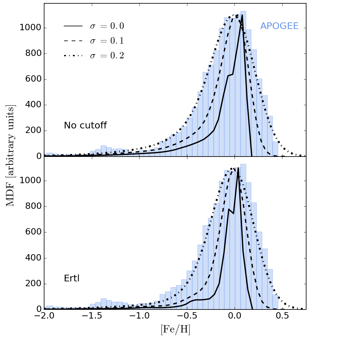
Our predicted metallicity distribution function (MDF), for the present choice of yields, is shown in the upper panel of Figure 4 and compared with the MDF we extracted from the APOGEE R12 dataset (Hayden et al. 2015; Shetrone et al. 2015; García Pérez et al. 2016). We chose APOGEE to maximize the statistics without having star duplication. To broaden our MDF, we convolved it with gaussian functions using different values for the standard deviation parameter, . In our case, this serves to mimic non-uniform mixing and stochastic processes that are not included yet in our one-zone model. This convolution process has been used before (e.g., Pilkington & Gibson 2012; Côté et al. 2013; Pilkington 2013) and shows that, with additional scatter, our predicted MDF could be in reasonable agreement with observations. But our narrow raw MDF (solid line in Figure 4) implies that our model currently does not capture the full complexity of the formation of the Milky Way, even if our model reproduces its current global properties (see Table 2). In particular, our model is probably not suited to reproduce the early evolution of the Galactic halo. But given the purpose of the present study, we still start our simulations with primordial gas in order to cover the metallicity range included in our stellar yields.
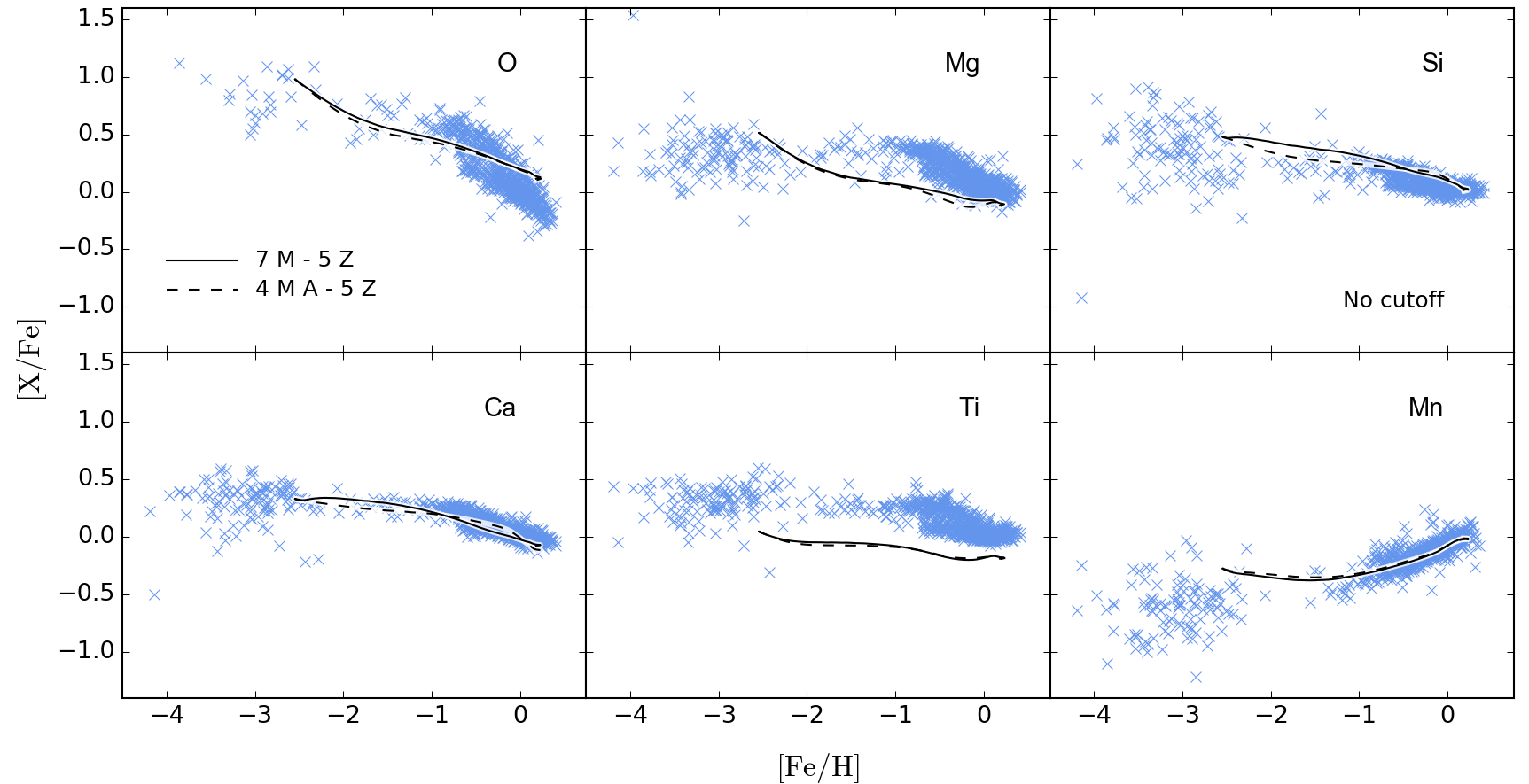
4.1 Mass and Metallicity Resolutions
Figure 5 presents our predictions for six elements, relative to Fe, against the stellar abundances observed in the Milky Way. For a given colour, the different line styles illustrate the impact of using different mass samplings and resolutions. For a given line style, the red and blue lines illustrate the impact of using different metallicity resolutions. With all the 14 metallicities sampled (blue lines), this last figure shows that different mass samplings produce different results when the number of masses is reduced to four (dashed and dot-dashed lines). At [Fe/H] , with the stellar yields used in this work, different selections of masses generate variations of about dex for O, Mg, and Ti, and dex for Si and Ca. At higher [Fe/H], our predictions are less sensitive to the selection of masses as variations are generally found within 0.1 dex. Within this [Fe/H] range, Ti and Mn are relatively insensitive to the mass resolution.
The variations seen at low [Fe/H] also highlight the impact of the mass range considered in the yields. The Mass Sampling A and B (see Table LABEL:tab_sample) include a maximum stellar mass of 25 and 30 M⊙, respectively. Those massive star models, for the lowest metallicity included in the yields, are the first to enrich the galactic gas at early time. Below [Fe/H] , the predictions generated by the Mass Sampling A and B (dashed and dot-dashed lines in Figure 5) therefore represent, respectively, the ejecta of the 25 and the 30 M⊙ models. In fact, we made a test where we modified the Mass Sampling A to include both the 25 and the 30 M⊙ models. In that case, for [Fe/H] , the dashed lines in Figure 5 became similar to the solid lines where all seven masses are sampled. However, above [Fe/H] , the variations between the different mass resolutions and samplings remained unchanged. This shows how sensitive our numerical predictions at early time are to the selection of the first stellar models that participate in the enrichment process.
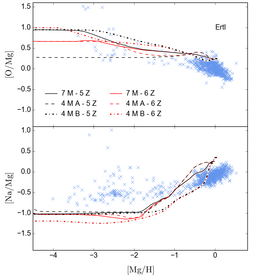
Reducing the number of metallicities does not produce any significant change in our numerical predictions, as shown by the red and blue lines in Figure 5. Figure 6 presents an analogous of Figure 5 but for the evolution of O and Na relative to Mg, as these three elements are all mainly produced during the pre-supernova phases. These predictions also converge toward the idea that the mass resolution and sampling are more important than the metallicity resolution. Indeed, in the case of Na, the different mass samplings generate more than 0.5 dex of variations at almost every [Mg/H] value, whereas reducing the number of metallicities only produce variations of about 0.1 dex.
We note that the variations seen for elements that do not match observations, such as Na and Ti, may not be representative, since we know stellar yields need to be examined in more details. However, we still decided to show these elements to highlight where improvements are needed in our stellar models.
4.2 Mass Resolution and Metallicity Range
Figure 7 shows the impact of using instead of
as the lower boundary of the metallicity range covered by our
set of yields. Because of the wide range of considered metallicities,
our yields interpolation scheme between the sampled metallicities
is done in the log space. This, unfortunately, prevents us from including
in the interpolation, as its logarithm value is not a finite number. Therefore,
when the zero-metallicity yields are included, we only
use them for stars formed in primordial gas, and switch to
as soon as the gas gets enriched by the first stellar
ejecta. In the case without the zero-metallicity yields, we use the
yields all the way until the metallicity of the gas
actually reaches , above which we interpolate between
metallicities.
When excluding the zero-metallicity yields (black
lines), the choice of the mass sampling has generally the biggest impact at
[Fe/H] , as opposed to [Fe/H] in the case where the
zero-metallicity yields are included (red lines). This suggests that
the lowest metallicity available in the yields plays a dominant role
in the numerical predictions at low [Fe/H]. As a matter of fact,
depending on the mass sampling, including or not the zero-metallicity
yields generally produces different results that do not converge
before reaching [Fe/H] of . The situation also
occurs when looking at the evolution of O and Na as a function of [Mg/H]
(Figure 8). The lowest [Fe/H] and [Mg/H] values
of our numerical predictions correspond to the first timestep that includes
chemical enrichment, and depend on the amount of Fe and Mg ejected
by the most massive stellar model sampled in the set of yields, for the
lowest metallicity. When excluding the zero-metallicity yields (black lines), the
relatively small variations at [Fe/H] , especially for O, Mg, and Si,
are due to a similarity in the ejecta composition of the 25 and 30 M⊙ models
at , which is the opposite in the models at .
4.3 Number of Masses in NuGrid Yields
NuGrid stellar yields currently include five metallicities (, 0.01, 0.006, 0.001, and 0.0001) and four models per metallicity for massive stars (, 15, 20, and M⊙). The question that ignited the present study was whether NuGrid should add more masses in their set of yields. To answer that question, we assumed that the current state of NuGrid could be represented by the Mass Sampling A - 5 Z sample (see Table LABEL:tab_sample) with the no-cutoff remnant mass prescription, as NuGrid does not for the moment consider islands of non-explodability. Figure 9 illustrates what would happen if seven masses were used instead of four.
For this comparison, we did not start our simulations with primordial composition. As shown in the previous sections, numerical predictions are significantly affected by the choice of stellar yields associated with the first stellar ejecta. To eliminate this complication, and to only focus on the current metallicity range covered by NuGrid, we started our simulations with the gas composition calculated in West & Heger (2013) for . Given this configuration, we conclude from Figure 9 that adding more masses is not a major concern for NuGrid. But still, the ideal case would be to provide a finer grid that do not produce variations when a few models are removed from the set of yields.
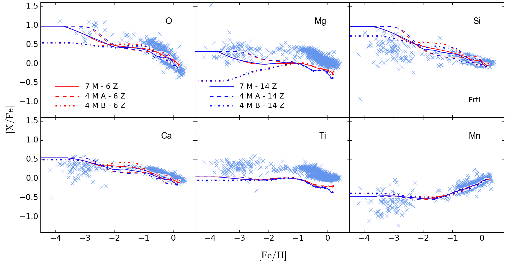
5 Yields with Islands of Non-Explodability
In this section we repeat the experiment made in the previous section, but using the set of yields generated with the remnant mass prescription of Ertl et al. (2015), which included islands of non-explodability. The adopted input parameters and our predicted MDF, for this choice of yields, are presented in Table 2 and in the lower panel of Figure 4, respectively. The MDFs generated with our two remnant mass prescriptions are roughly similar. The minor differences are due to different Fe ejection rates which are affected by the number of exploding models at a given time.
5.1 Mass and Metallicity Resolutions
Figure 10 shows the impact of the mass and metallicity resolutions using the remnant mass prescription of Ertl et al. (2015). At [Fe/H] below , the results with six and 14 metallicities are still indistinguishable. At [Fe/H] , for Mass Sampling B, the metallicity resolution only generates variations of 0.1 dex at most. At [Fe/H] , for Mass Sampling A, variations are generally between 0.05 dex and 0.15 dex, whereas almost no variation was seen with the no-cutoff prescription (see Figure 5).
In the case of Si, Ca, and Ti, the impact of the mass resolution at [Fe/H] is less important than with the no-cutoff prescription, as opposed to O and Mg which now show variations ranging from 0.4 dex to 0.7 dex. At [Fe/H] between and , the impact of the mass sampling is increased by about 0.1 dex relative to Figure 5. These results suggest that the mass requirement in a set of stellar yields depends on the remnant mass prescription and reinforce our conclusion that the mass resolution is more important than the metallicity resolution.
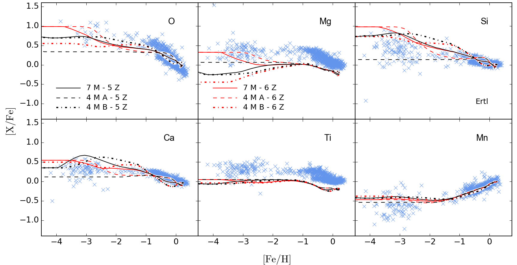
5.2 Mass Resolution and Metallicity Range
The first feature to notice in Figure 11 is the
importance of the mass sampling when only five masses and five
metallicities between 0.000153 and 0.0193 are considered (black dashed
and black dash-dotted lines). With the stellar yields used in this
work, this can generate variations up to dex for O and Mg,
and up to dex for Si and Ca across a larger [Fe/H]
interval than in the case with the no-cutoff prescription. Ti and Mn are
still insensitive to the mass sampling and resolution. Above [Fe/H]
, all predictions are relatively
insensitive to the mass resolution compared to the variations seen at low [Fe/H]. When plotted relative to Mg (see
Figure 12), O shows variations up to 0.6 dex at
[Mg/H] below , whereas Na shows variations up to 0.4 dex
at [Mg/H] above .
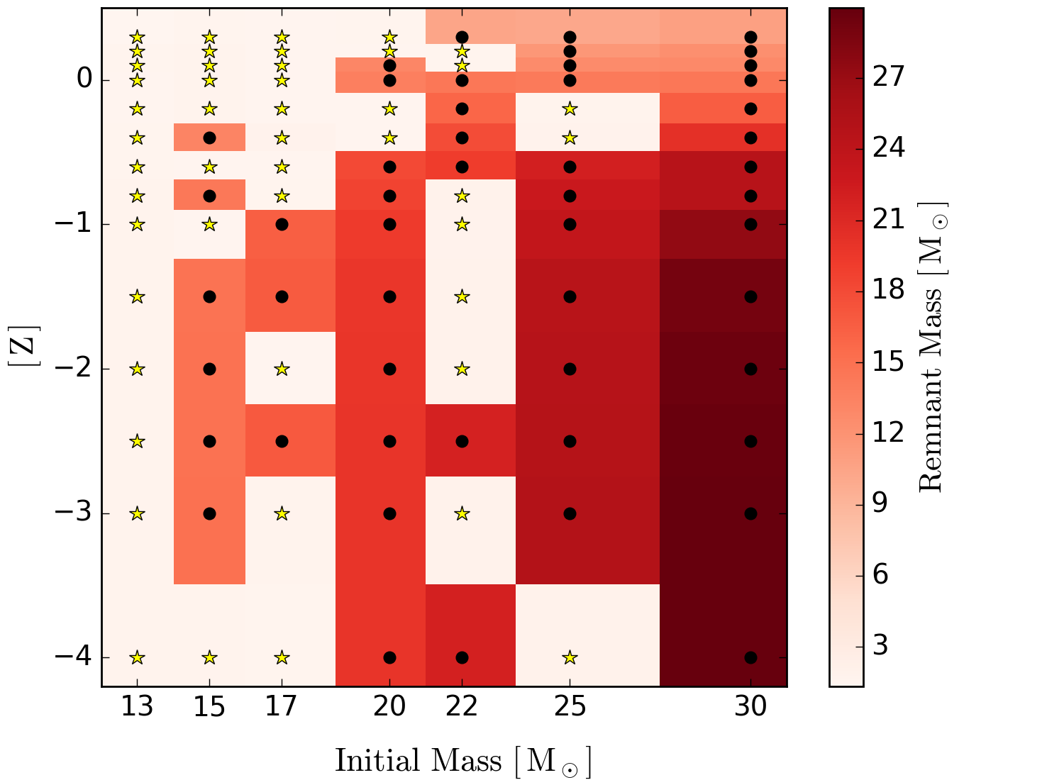
These significant variations are explained by the upper panel of
Figure 13. At , the islands of
non-explodability are regularly dispersed across the initial stellar
mass. With the Mass Sampling A, the whole selection consists of
non-exploding models, except for the M⊙ model. On the other
hand, the Mass Sampling B selects all the explosive models and misses
the islands of non-explodability located at M⊙,
M⊙, and M⊙. Therefore, when the stellar models at
are the first to enrich the primordial gas, the mass
resolution is crucial. The situation is less extreme at (see
the lower panel of Figure 13). But still, in order to
resolve the islands of non-explodability, the stellar models must be
judiciously sampled. For example, one could have a representative
selection without the M⊙ and M⊙ models, but not
without the M⊙ model.
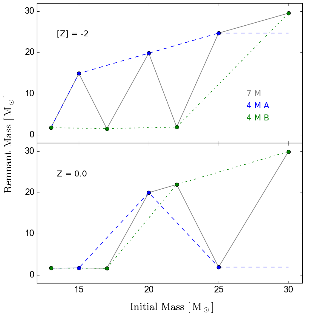
The different magnitudes of the impact of the mass sampling with and without the zero-metallicity yields, especially for Si and Ca, reinforces the idea that the lowest metallicity included in our set of stellar yields plays a major role in the numerical predictions at low [Fe/H]. In this case, even when all the seven masses are considered (solid lines), modifying the lowest metallicity available produces different results that do not converge before reaching [Fe/H] for O and Si, [Fe/H] for Mg, and [Fe/H] for Ca. This is consistent with observations and simulations that show a rapid increase of the average metallicity at early time in the Milky Way (e.g., Kobayashi & Nakasato 2011; Bensby et al. 2014).

Figure 14 shows an analogous of Figure 11
where we replaced , the lowest non-zero metallicity in our fiducial
case (middle panels), by (lower panels) and (upper panels).
The predictions generated using the zero-metallicity
yields (red lines) are still similar from one case to another below [Fe/H] , while variations
between cases (upper, middle, and lower panels) can be seen between [Fe/H] and . When the
zero-metallicity yields are not included (black lines), variations can be seen up to [Fe/H]
between the different cases, especially for Ca. The
black dashed lines are always flat and similar from one case to another since the Mass
Sampling A only selects one explosive model at , , and (see Figure 3).
Results shown in Figure 14 indicate once more that, below [Fe/H] ,
our numerical predictions are sensitive to the first stellar models that enrich the galactic gas.
However, we recall that we use a one-zone model that is
not necessarily suited to reproduce the Galactic halo, which
is associated with the metallicity range where most of the
variations occur.
It is worth remembering
that the two sets of yields used in the present work have been
calculated in the same way. The only ingredient responsible for the
differences between Figures 7 and 11 is the
remnant mass prescription, which suggests again that the mass
resolution required in stellar yields depends on the remnant mass
prescription used for massive stars. The stellar yields used in our experiment are not general. The fact
that the extreme case of is masked by the
zero-metallicity yields (see the comparison between the red and black lines
in Figure 11) does not mean the solution is to always use
zero-metallicity yields. Depending on the modeling assumptions, the
stellar evolutionary code, and the physics included, other sets of
yields could have different islands of explodability for their
zero-metallicity models (e.g., Sukhbold et al. 2015; Ertl et al. 2015). In that case, the
choice of the mass sampling could have different repercussions than
the ones shown in this section for the cases including zero-metallicity
yields.
The variations seen in our figures illustrate the potential of
our stellar yields to reproduce some of the observed scatter
at low [Fe/H], especially for O, Na, Mg, Si, and Ca. In inhomogeneous-mixing
chemical evolution models (e.g., Gibson et al. 2003; Argast et al. 2004; Cescutti et al. 2015; Wehmeyer et al. 2015), where the stellar initial mass function
is randomly sampled, individual stellar models can transfer their
ejecta into new generations of stars without being covered up
by all other stellar models that would be contributing when the
initial mass function is assumed to be fully sampled.
The level of scatter should
depends on the variety of abundance ratios seen in the ejecta of
the adopted stellar models. We are currently working on a stochastic version of our chemical evolution
codes to generate scatter in our predictions. This, however, is beyond
the scope of the present paper.
6 Summary and Conclusion
We used a single-zone model to address the question of how many masses
and metallicities are needed in a grid of stellar yields in order to
generate relevant and reliable predictions with chemical evolution
models. Using the set of stellar yields described in
Section 2.5, which has seven masses and 15 metallicities
for massive stars, we performed experiments where we extracted a
subset of models to evaluate the impact of the grid resolution on the
chemical evolution of seven elements. As a visual reference, we compared
our results with the stellar abundances observed in the Milky Way to
better appreciate the variations between our results. Our work
suggests that there is no general answer to how many masses and
metallicities are need for galactic chemical evolution applications.
The mass resolution needed in stellar yields depends on the element
considered and on the remnant mass prescription used for massive
stars. We found that yields with a monotonic remnant mass
distribution are generally more robust to modifications in the grid
resolution. Yields that possess islands of non-explodability are more
vulnerable, however, as explosive or non-explosive mass regimes can be
missed if not enough models are sampled. Our results suggest that the
yields from the lowest metallicity included in the grid can dominate
the chemical evolution up to [Fe/H] . Depending on the
remnant mass distribution applied for the lowest metallicities, a bad
mass sampling in the presence of islands of non-explodability can
cause variations that exceed 0.5 dex (see Figures 7 and 11).
The set of yields used in this work is not a general case and islands
of non-explodability could be found at different mass regimes in other
yields. Under different stellar modeling assumptions, it is not
excluded that extreme cases, such as the one at with the Ertl et al. (2015)
prescription (see Figure 13), could be associated with
other lower-metallicity or zero-metallicity yields.
We also studied the impact of the metallicity resolution and found that a wide range is more important than the number of metallicities. As for the mass resolution, yields with monotonic remnant masses are less affected by the metallicity resolution, reinforcing our conclusion that the grid resolution required in stellar yields depends on the remnant mass prescription and on the presence or absense of islands of non-explodability. Similar results likely would be found for any major discontinuities in yields as a function of initial mass.
acknowledgments
We are thankful to Anna Frebel for relevant discussions on stellar abundance observation. This research is supported by the National Science Foundation (USA) under Grant No. PHY-1430152 (JINA Center for the Evolution of the Elements), and by the FRQNT (Quebec, Canada) postdoctoral fellowship program. AH was supported by an ARC Future Fellowship (FT120100363). BWO was supported by the National Aeronautics and Space Administration (USA) through grant NNX12AC98G and Hubble Theory Grant HST-AR-13261.01-A. He was also supported in part by the sabbatical visitor program at the Michigan Institute for Research in Astrophysics (MIRA) at the University of Michigan in Ann Arbor, and gratefully acknowledges their hospitality. FH acknowledges support through a NSERC Discovery Grant (Canada). SB acknowledges support by JINA (ND Fund #202476).
References
- Asplund et al. (2009) Asplund M., Grevesse N., Sauval A. J., Scott P., 2009, ARA&A, 47, 481
- Argast et al. (2004) Argast D., Samland M., Thielemann F.-K., Qian Y.-Z., A&A, 416, 997
- Battistini & Bensby (2015) Battistini C., Bensby T., 2015, A&A, 577, 9
- Baugh (2006) Baugh C. M., 2006, RPPh, 69, 3101
- Bensby et al. (2014) Bensby T., Feltzing S., Oey M. S., 2014, A&A, 562, A71
- Bovy & Rix (2013) Bovy J., Rix H. W., 2013, ApJ, 779, 115
- Boylan-Kolchin et al. (2009) Boylan-Kolchin, M., Springel, V., White, S. D. M., Jenkins, A., & Lemson, G. 2009, MNRAS, 398, 1150
- Cayrel et al. (2004) Cayrel R., et al., 2004, A&A, 416, 1117
- Cescutti et al. (2015) Cescutti G., Romano D., Matteucci F., Chiappini C., Hirschi R., 2015, A&A, 577, 139
- Cohen et al. (2013) Cohen J. G., Christlieb N., Thompson I., McWilliam A., Shectman S., Reimers D., Wisotzki L., Kirby E., 2013, ApJ, 778, 56
- Cole et al. (2000) Cole S., Lacey C. G., Baugh C. M., Frenk C. S., 2000, MNRAS, 319, 168
- Côté et al. (2013) Côté B., Martel H., Drissen L., 2013, ApJ, 777, 107
- Côté et al. (2016b) Côté B., O’Shea B. W., Ritter C., Herwig F., Venn K. A., 2016b, arXiv:1604.07824
- Côté et al. (2016a) Côté B., Ritter C., O’Shea B. W., Herwig F., Pignatari M., Jones S., Fryer, C. L., 2016a, ApJ, 824, 82
- Chabrier (2003) Chabrier G., 2003, PASP, 115, 763
- Chiappini et al. (1997) Chiappini C., Matteucci F., Gratton R., 1997, ApJ, 477, 765
- Chiappini et al. (2001) Chiappini C., Matteucci F., Romano D., 2001, ApJ, 554, 1044
- Chieffi & Limongi (2004) Chieffi A., Limongi M., 2004, ApJ, 608, 405
- Chieffi & Limongi (2013) Chieffi A., Limongi M., 2013, ApJ, 764, 21
- De Donder & Vanbeveren (2004) De Donder E., Vanbeveren D., 2004, NewAR, 48, 861
- de Mink et al. (2013) de Mink S. E., Langer N., Izzard R. G., Sana H., de Koter A., 2013, ApJ, 764, 166
- Dunkley et al. (2009) Dunkley J., et al., 2009, ApJS, 180, 306
- Ekström et al. (2012) Ekström S., et al. 2012, A&A, 537, 146
- Ertl et al. (2015) Ertl T., Janka H.-Th., Woosley S. E., Sukhbold T., Ugliano M., 2015, ApJ, accepted (arXiv:1503.07522)
- Fakhouri et al. (2010) Fakhouri O., Ma C. P., Boylan-Kolchin M., 2010, MNRAS, 406, 2267
- Fenner et al. (2006) Fenner Y., Gibson B. K., Gallino R., Lugaro M., 2006, ApJ, 646, 184
- Ferrini et al (1992) Ferrini F., Matteucci F., Pardi C., Penco U., 1992, ApJ, 387, 151
- Flynn et al. (2006) Flynn C., Holmberg J., Portinari L., Fuchs B., Jahreiß H., 2006, MNRAS, 372, 1149
- García Pérez et al. (2016) García Pérez A. E., et al., 2016, AJ, 151, 144
- Gibson (2007) Gibson B. K., 2007, IAUS, 241, 161
- Gibson et al. (2003) Gibson B. K., Fenner Y., Renda A., Kawata D., Lee H.-c., 2003, PASA, 20, 401
- Hayden et al. (2015) Hayden M. R., et al., 2015, ApJ, 808, 132
- Heger et al. (2003) Heger A., Fryer C. L., Woosley S. E., Langer N., Hartmann D. H., 2003, ApJ, 591, 288
- Heger & Woosley (2010) Heger A., Woosley S. E., 2010, ApJ, 724, 341
- Hirschi (2007) Hirschi R., 2007, A&A, 461, 571
- Homma et al. (2015) Homma H., Murayama T., Kobayashi M. A. R., Taniguchi Y., 2015, ApJ, 799, 230
- Ishigaki et al. (2013) Ishigaki M. N., Aoki W., Chiba M., 2013, ApJ, 771, 67
- Ishigaki et al. (2012) Ishigaki M. N., Chiba M., Aoki W., 2012, ApJ, 753, 64
- Jacobson et al. (2015) Jacobson H. R., et al., 2015, ApJ, 807, 171
- Kauffmann et al. (1999) Kauffmann G., Colberg J. M., Diaferio A., White S. D. M., 1999, MNRAS, 303, 188
- Kennicutt (1998) Kennicutt R. C. Jr., 1998, ApJ, 498, 541
- Kobayashi & Nakasato (2011) Kobayashi C., Nakasato N., 2011, ApJ, 729, 16
- Kobayashi et al. (2006) Kobayashi C., Umeda H., Nomoto K., Tominaga N., Ohkubo T., 2006, ApJ, 653, 1145
- Kubryk et al. (2015) Kubryk, M., Prantzos, N., & Athanassoula, E. 2015, A&A, 580, 126
- Licquia & Newman (2015) Licquia T. C., Newman J. A., 2015, ApJ, 806, 96
- Limongi & Chieffi (2006) Limongi M., Chieffi A., 2006, ApJ, 647, 483
- Maoz et al. (2014) Maoz D., Mannucci F., Nelemans G., 2014, ARA&A, 52, 107
- Matteucci & Greggio (1986) Matteucci F., Greggio L., 1986, A&A, 154, 279
- McMillan (2011) McMillan P. J., 2011, MNRAS, 414, 2446
- Micali et al. (2013) Micali A., Matteucci F., Romano D., 2013, MNRAS, 436, 1648
- Minchev et al. (2013) Minchev I., Chiappini C., Martig M., 2013, A&A, 558, 9
- Mollá et al. (2015) Mollá M., Cavichia O., Gavilán M., Gibson B. K., 2015, MNRAS, 451, 3693
- Murray et al. (2005) Murray N., Quataert E., Thompson T. A., 2005, ApJ, 618, 569
- Nieuwenhuijzen & de Jager (1990) Nieuwenhuijzen H., de Jager C., 1990, A&A, 231, 134
- O’Connor & Ott (2011) O’Connor E., Ott C. D., 2011, ApJ, 730, 70
- Pagel (2009) Pagel B. E. J., 2009, Nucleosynthesis and Chemical Evolution of Galaxies (Cambridge University Press)
- Pardi et al. (1995) Pardi M. C., Ferrini F., Matteucci F., 1995, ApJ, 444, 207
- Pignatari et al. (2013) Pignatari M., et al., 2013, ApJS, submitted (arXiv:1307.6961)
- Pilkington (2013) Pilkington K., 2013, PhDT, 321
- Pilkington & Gibson (2012) Pilkington K., Gibson B. K., 2012, in Proc. XII Int. Symp. Nuclei in the Cosmos (NIC XII), 227
- Portinari et al. (1998) Portinari L., Chiosi C., Bressan A., 1998, A&A, 334, 505
- Rauscher et al. (2002) Rauscher T., Heger A., Hoffman R. D., Woosley S. E., 2002, ApJ, 576, 323
- Roederer et al. (2014) Roederer I. U., Preston G. W., Thompson I. B., Shectman S. A., Sneden C., Burley G. S., Kelson D. D., 2014, AJ, 147, 136
- Sana et al. (2012) Sana H., de Mink S. E., de Koter A., Langer N., Evans C. J., Gieles M., Gosset E., Izzard R. G., Le Bouquin J.-B., Schneider F. R. N., 2012, Science, 337, 444
- Schmidt (1959) Schmidt M., 1959, ApJ, 129, 243
- Shen et al. (2015) Shen S., Cooke R. J., Ramirez-Ruiz E., Madau P., Mayer L., Guedes J., 2015, ApJ, 807, 115
- Shetrone et al. (2015) Shetrone M., et al., 2015, ApJS, 221, 24
- Somerville & Davé (2015) Somerville R. S., Davé R., 2015, ARA&A, 53, 51
- Smartt (2009) Smartt S., 2009, ARA&A, 47, 63
- Springel et al. (2005) Springel, V., White, S. D. M., Jenkins, A., et al. 2005, Nature, 435, 629
- Springel et al. (2001) Springel V., White S. D. M., Tormen G., Kauffmann G., 2001, MNRAS, 328, 726
- Sukhbold & Woosley (2014) Sukhbold T., Woosley S. E., 2014, ApJ, 783, 10
- Sukhbold et al. (2015) Sukhbold T., Ertl T., Woosley S. E., Brown J. M., Janka H.-T., 2015, ApJ, submitted (arXiv:1510.04643)
- Thielemann et al. (1986) Thielemann F. K., Nomoto K., Yokoi K., 1986, A&A, 158, 17
- Travaglio et al. (2004) Travaglio C., Hillebrandt W., Reinecke M., Thielemann F. K., 2004, A&A, 425, 1029
- Ugliano et al. (2012) Ugliano M., Janka H.-T., Marek A., Arcones A., 2012, ApJ, 757, 69
- van de Voort et al. (2015) van de Voort F., Quataert E., Hopkins P. F., Kereš D., Faucher-Giguère C.-A., 2015, MNRAS, 447 140
- Weaver et al. (1978) Weaver T. A., Zimmerman G. B., Woosley S. E., 1978, ApJ, 225, 1021
- Wehmeyer et al. (2015) Wehmeyer B., Pignatari M., & Thielemann F. K., 2015, MNRAS, 452, 1970
- West & Heger (2013) West C., Heger A., 2013, ApJ, 774, 75
- West & Heger (in prep.) West C., Heger A., in prep.
- White & Frenk (1991) White S. D. M., Frenk C. S., 1991, ApJ, 379, 52
- Williams et al. (2014) Williams B. F., Peterson S., Murphy J., Gilbert K., Dalcanton J. J., Dolphin A. E., Jennings Z. G., 2014, ApJ, 791, 105
- Woosley & Heger (2007) Woosley S. E., Heger A., 2007, PhR, 442, 269
- Woosley et al. (2002) Woosley S. E., Heger A., Weaver T. A., 2002, RvMP, 74, 1015
- Woosley & Weaver (1995) Woosley S. E., Weaver T. A., 1995, ApJS, 101, 181
- Zhang et al. (2008) Zhang W., Woosley S. E., Heger A., 2008, ApJ, 679, 639