Bands in the spectrum of a periodic elastic waveguide

Abstract: We study the spectral linear elasticity problem in an unbounded periodic waveguide, which consists of a sequence of identical bounded cells connected by thin ligaments of diameter of order $h>0$. The essential spectrum of the problem is known to have band-gap structure. We derive asymptotic formulas for the position of the spectral bands and gaps, as $h\to 0$.

1. Introduction

We study the essential spectrum of the linearized elasticity system with traction–free boundary conditions in unbounded periodic waveguides denoted by $\Pi_{h}$. The waveguide, see Fig. 1.1, consists of infinitely many identical, translated bounded cells connected with small cylindrical ligaments, the length and radius of cross-section of which are both proportional to a small parameter $h>0$ so that the volume of the ligament is $O(h^{3})$. A number of papers (e.g [3], [31], [32]) has been devoted to geometrically similar waveguides consisting of arrays of macroscopic cells connected with thin structures, and, using rigorous perturbation arguments, the existence of gaps in the essential spectra has been detected. This has been done for elliptic boundary problems in elasticity, linear water-wave theory, piezo-electricity etc.

In this geometric setting the emerging of gaps is explained by that for small $h$, the problem can be seen as a perturbation of a ”limit spectral problem” ($h=0$) on a bounded domain, which consists of a single cell $\varpi_{0}$. The spectrum of such a problem is in general a sequence $(\lambda_{k})_{k=1}^{\infty}$ of eigenvalues , and the spectral bands of the original problem are situated ”close” to the eigenvalues $\lambda_{k}$. To analyse this closeness and its dependence on $h$ becomes a mathematical challenge: if that can be done accurately enough, one finds that disjoint eigenvalues correspond to spectral bands with a gap in between. In fact, this scheme can work only for a finite number of the lowest eigenvalues in the sense that for each fixed small $h$, at most a finite number of gaps can be found.

The purpose of this work is to refine the existing results by proving more accurate estimates than before for the end-points of spectral bands and gaps. For example, in [31] it was shown that for small $h$ and also $k$, the $k$th spectral band is situated within a distance $Ch$ from $\lambda_{k}$, the $k$th eigenvalue of the limit problem, where $C>0$ is a constant depending on the shape of the cells and on the physical constants of the elastic material, but not on the size of the small ligaments. In comparison, we shall find here an asymptotic formula for the spectral bands $\Upsilon_{k}$. Namely, by the Floquet-Bloch-theory of periodic problems, the bands are formed by eigenvalues $\Lambda_{k}^{h}(\eta)$ of the ”model problem” depending on the parameter $\eta\in[0,2\pi)$. It is in fact well known that the essential spectrum of the original problem (later (2.6)–(2.7)) equals

(1.1) $$\sigma_{\rm ess}=\bigcup_{k=1}^{\infty}\Upsilon_{k}^{h}\ ,\ \ \Upsilon_{k}^{h}=\{\Lambda_{k}^{h}(\eta)\,:\,\eta\in[0,2\pi)\}.$$

In Theorem 4.1, see (4.1), (4.2), we determine the first order (in $h$) correction term for the difference of $\Lambda_{k}^{h}(\eta)$ and $\lambda_{k}$. The result includes the following claim:

For all $k$ we have the estimate

(1.2) $$\big{|}\Lambda_{k}^{h}(\eta)-(\lambda_{k}+h\Lambda_{k}^{\prime}(\eta))\big{|}\leq C_{k}h^{3/2}\ \ \forall h>0\ ,\ \eta\in[0,2\pi),$$

where

(1.3) $$\Lambda_{k}^{\prime}(\eta)=2a\lambda_{k}+\big{(}A_{k}+e^{i\eta}B_{k}\big{)}^{\top}{\bf M}^{+}\big{(}A_{k}+e^{-i\eta}B_{k}\big{)},$$

the column vectors $A_{k}$, $B_{k}\in{\mathbb{R}}^{3}$ and the positive definite matrix ${\bf M}^{+}\in{\mathbb{R}}^{3\times 3}$ do not depend on $h$ or $\eta$, and the number $a$ equals $0$ or $1$ (according to the domain, see Section 2.1).

The quantities $A_{k}$, $B_{k}$, ${\bf M}^{+}$ will be determined in Sections 3.2, 3.3. Anyway, the coefficient $\Lambda_{k}^{\prime}(\eta)$ of the correction term depends only on the geometry of the limit problem. (It might thus be desirable to provide numerical experiments on the effect of this coefficient and the geometry of the limit domain to the appearance of spectral gaps, but we do not provide such information here.) However, information on the position and length of $\Upsilon_{k}$ obtained here is much more precise than before, since until now there has not even existed a criterion to distinguish, if the band has positive length or it consists of only a single point, which is an eigenvalue of infinite multiplicity. In many cases the vector $B_{k}$ is nonzero, and it follows from (1.3) that length of the band $\Upsilon_{k}^{h}$ is positive.

In addition, we find an asymptotic representation for the corresponding eigenfunctions $U_{k}^{h}$ of the model problem, which includes the leading terms both near the junctions of the periodicity cells and at a distance of these points. Since it is difficult to describe this without a number of definitions, we refer to Theorem 4.1 for details.

In literature spectral gaps in essential spectra for scalar equations and Maxwell’s system in infinite periodic media have been considered in many papers, see for example [7], [8], [9], [12], [13], [34]. For results on gaps in (quasiperiodic, unbounded) waveguides we mention the papers [2], [6], [10], [24]; for an approach based on parameter–dependent Korn–type inequalities, see [5], [25], [26], [28], [27]. A comparison of the present work with the paper [31] was already presented above. We just mention that the method of [31] is based on the max-min principle for eigenvalues. We finally also mention the paper [3], which contains an analysis of spectral bands much like in the present work, but in the more simple setting of the linear water wave equation.

As for the structure of this paper, we present in Section 2 the geometry of the waveguide $\Pi_{h}$, the formulation of the linear spectral elasticity problem and its variational formulation. The parameter dependent problem arising from the FBG-transform is presented in Section 2.2, together with the variational formulation in a special Sobolev-type Hilbert space ${\mathcal{H}}^{h,\eta}$. The limit problem is studied in Section 2.3, and additional technical devices are introduced in Section 2.4. Section 3 contains the formal asymptotic analysis, in particular the construction of the asymptotic ansätze for the eigenfunctions of the model problem. Section 4.1 contains the main result, and proof is given in Sections 4.2–4.3. One point of the proof needs the existence of spectral gaps, which can be obtained by an adaptation of the method [31]; this is presented in the appendix, Section 5.

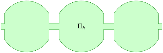
Figure 1.1. The waveguide $\Pi_{h}$

Acknowledgement. The authors want to thank Prof. Sergei A. Nazarov for many discussions on the topic of this work.

2. Problem formulation, band-gap spectrum and limit problem

2.1. Spectral elasticity problem in the waveguide.

The problem domain is a periodic waveguide $\Pi_{h}$, Fig. 1.1, depending on a small geometric parameter $h\in(0,\frac{1}{10}]$ and consisting of infinitely many disjoint translated copies of a bounded cell connected by thin cylinder. Let us describe the exact definition. We denote by $\varpi_{\bullet}$ a bounded domain in ${\mathbb{R}}^{3}$ containing the points $P^{\pm}=(0,0,\pm 1/2)$ in its interior, such that

(2.1) $$\varpi_{0}=\{x=(x_{1},x_{2},x_{3})=(y,z)\in\varpi_{\bullet}\,:\,y\in{\mathbb{R}^{2}},|z|<1/2\}$$

is a domain with Lipschitz boundary $\partial\varpi_{0}$. Notice that in a neighbourhood of the points $P^{\pm}$ the boundary $\partial\varpi_{0}$ is ”flat”: it consists of an open subset of the plane $\{(y_{1},y_{2},\pm 1/2)\}$.

We also denote by $\theta\subset{\mathbb{R}}^{2}$ a bounded domain which has Lipschitz boundary $\partial\theta$ and which is star-shaped with respect to the point $(0,0)\in\theta$. (Any point of $\theta$ can be joined with $(0,0)$ by a line segment running in $\theta$.) We also denote for $h>0$

$$\theta_{h}=h\theta=\{hy\in{\mathbb{R}}^{2}:y\in\theta\}.$$

By a thin cylinder we mean the set $\Theta_{h}=\theta_{h}\times{\mathbb{R}}$.

We fix a number $a$ to be either 0 or 1 (see below for a discussion) and denote by $a_{h}$ the number $(1-ah)^{-1}\in{\mathbb{R}}$ and also the multiplier $a_{h}:x\mapsto(1-ah)^{-1}x$ in any space ${\mathbb{R}}^{n}\ni x$, $n\in{\mathbb{N}}$. The meaning will be clear from the context. Let us define a scaled, translated family of bodies

(2.2) $$\varpi(j,h)=\{x:a_{h}(y,z-j)\in\varpi_{0}\}\ \ \mbox{with}\ \varpi(h):=\varpi(0,h)=a_{h}^{-1}(\varpi_{0}),$$

see Fig. 2.1. The periodicity cell $\varpi_{h}\supset\varpi(h)$, Fig. 2.2, is the set

(2.3) $$\varpi_{h}=\varpi(h)\cup\Big{(}\theta_{h}\times\big{(}-\frac{1}{2},\frac{1}{2}\big{)}\Big{)},$$

in other words, $\varpi_{h}$ is the disjoint union of $\varpi(h)$ and the small sets

(2.4) $$\Theta_{h}^{-}=\theta_{h}\times(-1/2,-1/2+ah/2],\quad\Theta_{h}^{+}=\theta_{h}\times(1/2-ah/2,1/2].$$

Finally, the waveguide $\Pi_{h}$, Fig. 1.1, is defined as

(2.5) $$\Pi_{h}=\Theta_{h}\cup\bigcup_{j\in{\mathbb{Z}}}\varpi(j,h).$$

Note that when $h=0$, the waveguide $\Pi_{h}$ becomes a union of disconnected sets.

If $a=0$ above, then of course $a_{h}=1$ is independent of $h$, and the cells $\varpi(j,h)$ contact each other: the cylinder $\Theta_{h}$ loses its role and the cells are connected by holes, ”apertures” of diameter $h$ in their boundaries. In this case also the volume of the periodicity cells is independent of $h$. The subsequent calculations are concentrated on treating the case $a=1$. In many cases the calculations are unnecessarily complicated for $a=0$, but that case can be considered as a by-product; some details will be omitted, and the reader is asked to keep it also in mind. If $a=1$, the diameter of the connecting ligaments is of order $h$ and the volume is proportional $h^{3}$. This means a certain difference to the related paper [31].

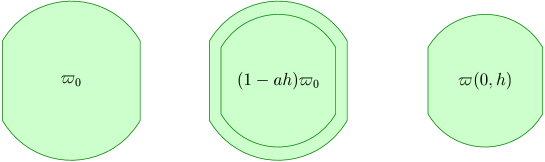
Figure 2.1. Transformation of the set $\varpi_{0}$

Figure 2.2. Periodicity cell $\varpi_{h}$

We consider the spectral elasticity problem in $\Pi_{h}$ written in matrix form, cf. [19], [29]. This is formulated for an unknown ${\mathbb{R}}^{3}$-valued vector function $u(x)$, which describes the displacement vector of the given material. The system contains a first order differential operator matrix $D(\nabla_{x})$, where $\nabla_{x}$ denotes the gradient with respect to the variable $x$ and

$$D(x)=\left(\begin{array}[]{cccccc}x_{1}&0&2^{-1/2}x_{2}&2^{-1/2}x_{3}&0&0\\ 0&x_{2}&2^{-1/2}x_{1}&0&2^{-1/2}x_{3}&0\\ 0&0&0&2^{-1/2}x_{1}&2^{-1/2}x_{2}&x_{3}\end{array}\right)^{\top}\,,\quad x=(x_{1},x_{2},x_{3})^{\top}\,,$$

and a matrix $A$ of dimension $6\times 6$, describing elastic moduli. The matrix $A$ is assumed to be positive definite and, for technical simplicity, constant. The problem can be written as

(2.6) $$L_{x}u(x) = \lambda u(x)\ ,\ \ x\in\Pi_{h},$$

(2.7) $${N_{x}^{h}}u(x) = 0\ \mbox{for a.e.}\ x\in\partial\Pi_{h}\,,$$

where

(2.8) $$L_{x}=D(-\nabla_{x})^{\top}AD(\nabla_{x})\ ,\ \ {N_{x}^{h}}=D(\nu(x))^{\top}AD(\nabla_{x})\ ,$$

$\nu$ is the outward normal vector defined for almost all points of the Lipshitz surface $\partial\Pi_{h}$ and $\lambda$ is a spectral parameter. The boundary operator ${N_{x}^{h}}$ depends on $h$ via the domain $\Pi_{h}$. (Later on, $\nu$ will always denote the outward normal of a boundary, which will be clear from the context.) Also, $L_{x}$ is just a constant coefficient partial differential operator containing only second order terms. In general, $\lambda$ could be multiplied in (2.6) by a fixed function describing the material density, but we assume this function to be equal to 1 for simplicity.

The variational formulation of the spectral problem (2.6)-(2.7) reads as

(2.9) $$a(u,v;\Pi_{h})=\lambda(u,v)_{\Pi_{h}},\quad v\in H^{1}(\Pi_{h})^{3}.$$

Here, given a regular enough domain $\Omega\subset{\mathbb{R}}^{3}$, we use the notation

(2.10) $$a(f,g;\Omega)=(AD(\nabla_{x})f,D(\nabla_{x})g)_{\Omega}\ ,\ \mbox{and}\ \ (f,g)_{\Omega}=\sum_{j=1}^{k}\int\limits_{\Omega}f\overline{g}dx$$

for the usual (complex valued) inner product in $L^{2}(\Omega)^{k}$, $k=1,2,3$; the latter notation will also be used for domains in ${\mathbb{R}}^{2}$. We denote the standard Sobolev space of first order on $\Omega$ by $H^{1}(\Omega)$. The bilinear form (2.10) is positive and closed in the Sobolev space $H^{1}(\Pi_{h})^{3}$ and consequently (see [4]) our problem can be rewritten as an abstract operator equation ${\mathcal{T}}^{h}u=\lambda u$, where ${\mathcal{T}}^{h}$ is an unbounded, self-adjoint densely defined operator in the Hilbert space $L^{2}(\Pi_{h})^{3}$ and thus the spectrum $\sigma({\mathcal{T}}^{h})\ni\lambda$ is a subset of $\overline{{\mathbb{R}}_{+}}=[0,+\infty)$. The embedding $H^{1}(\Pi_{h})\subset L^{2}(\Pi_{h})$ is not compact due to the unboundedness of the domain $\Pi_{h}$, hence, the essential spectrum $\sigma_{\rm{ess}}({\mathcal{T}}^{h})$ is not empty (see [4], Th.10.15). Finally, spectral concepts of the problem (2.6)–(2.7) are defined with the help of the operator ${\mathcal{T}}^{h}$. In particular, $\sigma_{\rm{ess}}:=\sigma_{\rm{ess}}({\mathcal{T}}^{h})$.

2.2. Floquet-Bloch-Gelfand transform and essential spectrum.

To analyse the band-gap structure spectrum of the problem (2.6)–(2.7) we use the FBG-transform

$$v(y,z)\mapsto\ V(y,z;\eta)=\frac{1}{\sqrt{2\pi}}\sum_{j\in\mathbb{Z}}\exp(-i\eta j)v(y,z+j),$$

where $(y,z)\in\Pi_{h}$ on the left, while $\eta\in[0,2\pi)$ and $(y,z)\in\varpi_{h}$ on the right. As well known, this operator establishes an isometric isomorphism between Lebesgue spaces $L^{2}(\Pi_{h})^{3}$ and $L^{2}(0,2\pi;L^{2}(\varpi_{h})^{3}),$ where $L^{2}(0,2\pi;B)$ is the Lebesgue space of functions with values in the Banach space $B$, endowed with the norm $\|V;L^{2}(0,2\pi;B)\|^{2}=\int_{0}^{2\pi}\|V(\eta);B\|^{2}d\eta\,.$ The FBG-transform is also an isomorphism from the Sobolev space $H^{1}(\Pi_{h})^{3}$ onto $L^{2}(0,2\pi;H^{1}_{\eta}(\varpi_{h})^{3})$ and from $H^{2}(\Pi_{h})^{3}$ onto $L^{2}(0,2\pi;H^{2}_{\eta}(\varpi_{h})^{3})$. Here, for a fixed $h$ and $\eta$, the space $H^{2}_{\eta}(\varpi_{h})$ is the space of Sobolev functions $f$ on $\varpi_{h}$, which satisfy quasiperiodicity conditions

(2.11) $$\ \ f(y,1/2) = e^{i\eta}f(y,-1/2)\ ,\ \ \partial_{z}f(y,1/2)=e^{i\eta}\partial_{z}f(y,-1/2)\ ,\ \ y\in\theta_{h}.$$

Similarly, the space $H^{1}_{\eta}(\varpi_{h})$ consists of $H^{1}$-functions satisfying the condition (2.11) only. In the following we denote by ${\mathcal{H}}^{h,\eta}$ the space $H^{1}_{\eta}(\varpi_{h})^{3}$ endowed with the norm $\|f;{\mathcal{H}}^{h,\eta}\|$ coming from the inner product

(2.12) $$\langle f,g\rangle_{{\mathcal{H}}^{h,\eta}}=(f,g)_{\varpi_{h}}+\big{(}AD(\nabla_{x})f,D(\nabla_{x})g\big{)}_{\varpi_{h}};$$

notice that the last form on the right is Hermitian and positive on $H^{1}_{\eta}(\varpi_{h})^{3}$. Obviously, $\|f;{\mathcal{H}}^{h,\eta}\|\leq C\|f;H^{1}(\varpi_{h})\|$ for some constant independent of $h$ and $\eta$, since the matrix $A$ was assumed to be constant.

Lemma 2.1.

The norm $\|\cdot;{\mathcal{H}}^{h,\eta}\|$ is equivalent to $\|\cdot;H^{1}(\varpi_{h})\|$ with constants independent of $h>0$ and $\eta\in[0,2\pi)$.

Proof. It is enough to show that the Korn inequality

(2.13) $$\|f;H^{1}(\varpi_{h})\|^{2}\leq C\big{(}\|f;L^{2}(\varpi_{h})\|^{2}+\big{(}AD(\nabla_{x})f,D(\nabla_{x})f\big{)}_{\varpi_{h}}$$

holds for Sobolev-functions $f$ in such a way that the constant $C>0$ can be chosen independently of $h$, $\eta$. It is quite obvious that replacing $\varpi_{h}$ by $\varpi(h)$ (see (2.2)) in (2.13), the corresponding inequality would hold with constant independent of $h$, $\eta$. But the same is true also, when $\varpi_{h}$ is replaced by the two sets $\Theta_{h}^{\pm}$, see (2.4). This follows from the result [16], Th. 1, Th. 2. For example the set $\Theta_{h}^{+}$ has diameter $c_{1}h$ and it is in the terminology of the citation starshaped with respect to a ball with center in $(0,0,1/2-ah/4)$ and radius $c_{2}h$, where $c_{1}$, $c_{3}$ do not depend on $h$ (see the assumptions on $\theta$ in Section 2.1). Then, (2.13) follows by combining these facts.   $\Box$

Using the FBG-transform the problem (2.6)-(2.7) turns into a model problem on the periodicity cell for the unknown $U=U(x;\eta)$,

(2.14) $$\overline{D(-\nabla_{y},-\partial_{z}-i\eta)}^{\top}AD(\nabla_{y},\partial_{z}+i\eta)U=\Lambda U\ \ \ \mbox{in}\ \varpi_{h},$$

(2.15) $$\overline{D(\nu(x))}^{\top}AD(\nabla_{y},\partial_{z}+i\eta)U=0\ \ \ \mbox{ a.e. in}\ \partial\varpi_{h}\setminus(\theta_{h}^{-}\cup\theta_{h}^{+})\,,$$

(2.16) $$U(y,1/2;\eta)=e^{i\eta}U(y,-1/2;\eta),\quad y\in\theta_{h}\,,$$

(2.17) $$\partial_{z}U(y,1/2;\eta)=e^{i\eta}\partial_{z}U(y,-1/2;\eta),\quad y\in\theta_{h}\,,$$

where the overline denotes complex conjugation and $\Lambda$ is a spectral parameter. In the weak form this amounts to finding $0\not=U\in{\mathcal{H}}^{h,\eta}$ and $\Lambda\in{\mathbb{C}}$ with

(2.18) $$a(U,V;\varpi_{h})=\Lambda(U,V)_{\varpi_{h}}$$

for all $V\in{\mathcal{H}}^{h,\eta}$. The problem (2.14)-(2.17) can be associated with a self-adjoint, positive and compact operator $\mathcal{B}^{h,\eta}:{\mathcal{H}}^{h,\eta}\to{\mathcal{H}}^{h,\eta}.$ We define ${\mathcal{B}}^{h,\eta}$ in a standard way by requiring that the identity

(2.19) $$\langle{\mathcal{B}}^{h,\eta}U,V\rangle_{{\mathcal{H}}^{h,\eta}}=(U,V)_{\varpi_{h}}$$

holds for all $U,V\in{\mathcal{H}}^{h,\eta}$. The problem (2.18) is then equivalent to the spectral problem ${\mathcal{B}}^{h,\eta}U=\mu U$ with a new spectral parameter $\mu=(1+\Lambda)^{-1}$. The spectrum of ${\mathcal{B}}^{h,\eta}$ consists of a decreasing sequence $\{\mu_{k}^{h}(\eta)\}_{k\geq 1}$ of eigenvalues and the point 0 of the essential spectrum. As a consequence, the spectrum of the problem (2.14)-(2.17) can be presented as the eigenvalue sequence (counting multiplicities)

(2.20) $$0\leq\Lambda_{1}^{h}(\eta)\leq\Lambda_{2}^{h}(\eta)\leq\ldots\leq\Lambda^{h}_{p}(\eta)\leq\ldots\to+\infty.$$

We denote the corresponding eigenfunctions by $U^{h}_{p}\in H^{1}_{\eta}(\varpi_{h})^{3}$, where the dependence on $\eta$ will usually not be shown. We require the orthogonality property

(2.21) $$(U^{h}_{p},U^{h}_{q})_{\varpi_{h}}=\delta_{p,q},\quad p,q=1,2,\ldots.$$

By [11], [17], [21], [23], [30], Theorem 3.4.6, [31], Theorem 2.1), for example, a number $\Lambda$ belongs to the resolvent set or the discrete spectrum of ${\mathcal{T}}^{h}$ (end of Section 2.1), if and only if it does not coincide with $\Lambda_{p}^{h}(\eta)$ for any $\eta\in[0,2\pi]$ and $p$. Hence, the essential spectrum of ${\mathcal{T}}^{h}$ and thus also of the original problem (2.6)–(2.7) have band-gap structure (1.1),

(2.22) $$\sigma_{{\rm ess}}({\mathcal{T}}^{h})=\bigcup_{p=1}^{\infty}\Upsilon_{p}^{h},=\bigcup_{p=1}^{\infty}\{\Lambda_{p}^{h}(\eta):\eta\in[0,2\pi)\};$$

where the spectral bands $\Upsilon_{p}^{h}$ are closed intervals (possibly single points).

2.3. Spectrum of the limit model problem

When $h\to 0$, the cylinder $\Theta_{h}$ turns into a negligible set and the quasi-periodicity conditions (2.16)-(2.17) lose their meaning. The model problem (2.14)-(2.17) turns into the so called limit problem on the isolated elastic body $\varpi_{0}$,

(2.23) $$D(-\nabla_{x})^{\top}AD(\nabla_{x})u=\Lambda^{0}u\ \ \mbox{in}\ \varpi_{0},$$

(2.24) $$D(\nu(x))^{\top}AD(\nabla_{x})u=0\ \ \mbox{ a.e.\,in}\ \partial\varpi_{0}\,,$$

where $u$ is the unknown function on $\varpi_{0}$ and $\Lambda^{0}$ is a spectral parameter. The problem has for any $\eta\in(0,2\pi]$ the same eigenvalues as the case $\eta=0$, so we can restrict to this single limit case, see [31] for some more details. We again denote by $a(u,v;\varpi_{0})$ the sesquilinear form corresponding to the problem (2.23)-(2.24). It is positive and closed on $H^{1}(\varpi_{0})^{3}$. We also define the space ${\mathcal{H}}^{0}$ (with no quasiperiodicity conditions) and the self-adjoint, positive, compact operator ${\mathcal{B}}^{0}:{\mathcal{H}}^{0}\to{\mathcal{H}}^{0}$, associated to the problem (2.23)–(2.24), analogously to ${\mathcal{H}}^{h,\eta}$ and ${\mathcal{B}}^{h,\eta}$ of the previous section. Since $\varpi_{0}$ is a bounded Lipschitz domain, the limit problem has an eigenvalue sequence

(2.25) $$0=\lambda_{1}=\ldots=\lambda_{6}<\lambda_{7}\leq\lambda_{8}\leq\ldots\leq\lambda_{p}\leq\ldots\to+\infty.$$

Here the $\lambda_{1}$, …, $\lambda_{6}$ are the eigenvalues of the rigid motions including three translations and rotations. For every $p$, let $u_{p}$ be the eigenfunction corresponding to $\lambda_{p}$, normalized in $L^{2}(\varpi_{0})^{3}$ by

(2.26) $$(u_{p},u_{q})_{\varpi_{0}}=\delta_{p,q},\quad p,q=1,2,\ldots$$

We also state a scaled version of the problem (2.23)–(2.24) (see (2.2)):

(2.27) $$D(-\nabla_{x})^{\top}AD(\nabla_{x})u=\Lambda^{0}u\ \ \mbox{ in}\ \varpi(h),$$

(2.28) $$D(\nu(x))^{\top}AD(\nabla_{x})u=0\ \ \mbox{ a.e.\,in}\ \partial\varpi(h)\,.$$

It is a trivial consequence of the above remarks that the eigenvalues and corresponding eigenvectors of (2.27)–(2.28) are now given by

(2.29) $${\lambda_{j}^{h}}:=a_{h}^{2}\lambda_{j}=\lambda_{j}+O(h)\ ,\ \ {u_{j}^{h}}(x):=a_{h}^{3/2}u_{j}(a_{h}x),$$

and the relation $({u_{j}^{h}},u_{k}^{h})_{\varpi(h)}=\delta_{j,k}$ still holds.

Lemma 2.2.

There exist $b_{1}>0$ such that for all $k\in{\mathbb{N}}$, the bounds $|u_{k}(x)|\leq C_{k}\ ,\ |\nabla u_{k}(x)|\leq C_{k}$ hold for $x\in\varpi_{0}\subset{\mathbb{R}}^{3}$ with $|x-P^{\pm}|<b_{1}$.

The proof of this fact follows from standard local elliptic estimates and our smoothness assumption of the boundary $\partial\varpi_{0}$ near the points $P^{\pm}$, see (2.1). The lemma is proven in detail in [31], Lemma 3.1. As a corollary, we also have

(2.30) $$|{u_{k}^{h}}(x)|\leq C_{k}\ ,\ |\nabla{u_{k}^{h}}(x)|\leq C_{k}$$

for all small enough $h>0$, for all $x\in\varpi(h)$ with $|x-P^{\pm}|<b_{1}$.

2.4. Additional notation.

We finish this section by fixing some more notation. We write in any dimension $n$, $B(x_{0},r)=\{x\in{\mathbb{R}}^{n}\,:\,|x-x_{0}|<r\}\subset{\mathbb{R}}^{n}$ and $A(s,r)=\{x\in{\mathbb{R}}^{n}\,:\,s<|x|<r\}\subset{\mathbb{R}}^{n}$ for $0<s<r$, and $e^{(j)}\in{\mathbb{R}}^{n}$, $j=1,\ldots,n$, for the canonical basis vectors.

We define some smooth cut-off functions to be used at several points later. First, let $\chi_{\theta}:{\mathbb{R}}^{3}\to[0,1]$ be a $C^{\infty}$-smooth function equal to 1 on the set $\theta\times[-1,1]$ and equal to 0 outside some neighbourhood of this set. More precisely, we assume that $\chi_{\theta}$ is chosen such that

(2.31) $$\varpi_{h}\cap\{x\,:\,\mathcal{X}^{h}_{+}(x)<1\}\subset\varpi(h)\ \ \mbox{and}\ \ \varpi_{h}\cap\{x\,:\,\mathcal{X}^{h}_{-}(x)<1\}\subset\varpi(h).$$

for all $h\in(0,\frac{1}{10}]$, where $\mathcal{X}^{h}_{\pm}(x)=\chi_{\theta}(h^{-1}(x-P^{\pm}))$ . We also set for $x\in{\mathbb{R}}^{3}$

(2.32) $$\mathcal{X}^{h}(x)=1-\mathcal{X}^{h}_{-}(x)-\mathcal{X}^{h}_{+}(x),$$

As a consequence,

(2.33) $$\varpi_{h}\cap\mbox{supp}\,\mathcal{X}^{h}\subset\varpi(h)\ \ \mbox{and}\ \ |\nabla{\mathcal{X}}^{h}|\leq{C}{h^{-1}},$$

and ${\mathcal{X}}^{h}$ equals 0 in both balls $B(P^{\pm},ch)$ and 1 outside the balls $B(P^{\pm},c_{1}h)$ for some constants $0<c<c_{1}$. Also, notice that at least for small enough $h$, the boundary $\partial\varpi(h)$ is infinitely smooth (planar) and (2.30) holds inside the domain $\{x\in{\mathbb{R}}^{3}\;:\,{\mathcal{X}}^{h}(x)<1\}.$

We also denote $\chi_{\pm}:{\mathbb{R}}^{3}\to[0,1]$ some $C^{\infty}$-cut-off functions such that

(2.34) $$\chi_{\pm}(x)=1\ \mbox{for}\ x\in B(P^{\pm},S)\ \ \mbox{and}\ \ \chi_{\pm}(x)=0\ \mbox{for}\ x\notin B(P^{\pm},R);$$

for some $0<S<R<1/2$. Obviously, $\chi_{+}(y,z)=0$ for $z\leq 0$ and $\chi_{-}(y,z)=0$ for $z\geq 0$ and also for small enough $h$,

(2.35) $$\chi_{\pm}{\mathcal{X}}^{h}_{\pm}={\mathcal{X}}^{h}_{\pm}$$

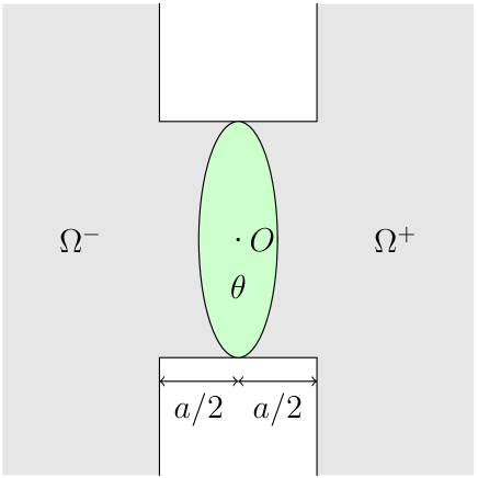
Figure 2.3. The set $\Omega$.

We define for $a\in\{0,1\}$ the domains

$$\Omega := \{\xi\in\mathbb{R}^{3}\,:\,|\xi_{3}|>a/2\}\cup\big{(}\theta\times[-a/2,a/2]\big{)}\ \ \mbox{and }$$

(2.36) $$\Omega^{\pm} = \{\xi\in\Omega:\,\,\pm\xi_{3}>0\},$$

see Fig. 2.3. The reader should keep in mind that if $x\in\varpi_{h}\cap{\rm supp}\,\chi_{\pm}$, then $\xi=h^{-1}(x-P^{\pm})\in\Omega^{\mp}$. We define the coordinate change mappings $\tau_{\pm}^{h}(x)=(x-P^{\pm})/h$ and denote $\tau_{\pm}:=\tau_{\pm}^{1}$.

3. Formal asymptotic procedure

3.1. The ansätze, the first step.

In this section we present asymptotic formulas as $h\to 0$, for the eigenvalues $\Lambda_{k}^{h}(\eta)$ and for the eigenfunctions $U_{k}^{h}$, see (2.20), (2.21) and (3.1), (3.1). We start with the case that an eigenvalue $\lambda_{k}$ of the limit problem is simple, see (2.25). Let us fix such a $k$.

As for the corresponding eigenvalue $\Lambda_{k}^{h}(\eta)$ of the model problem (2.14)–(2.17), we expect it to be a perturbation of $\lambda_{k}$, and the asymptotic formula or ansatz is written as

(3.1) $$\Lambda_{k}^{h}(\eta) = \lambda_{k}+h\Lambda_{k}^{\prime}(\eta)+\widetilde{\Lambda}_{k}^{h}(\eta),$$

where $\Lambda_{k}^{\prime}(\eta)$ is the main correction term, to be calculated in Section 3.3, and $\widetilde{\Lambda}_{k}^{h}(\eta)$ is a remainder, which will be shown to be of small order $O(h^{3/2})$ in Section 4. Next, we introduce the following asymptotic formula for the eigenfunction $U_{k}^{h}$,

$$U_{k}^{h}(x) = \mathcal{X}^{h}(x)\Big{(}u_{k}(a_{h}x)+hu_{k}^{\prime}(a_{h}x))\Big{)}$$

$$+ \sum_{\pm}\chi_{\pm}(x){{V_{k}^{\mp}}}(h^{-1}(x-P^{\pm}))-\sum_{\pm}\chi_{\pm}(x)\mathcal{X}^{h}(x)u_{k}(P^{\pm})$$

$$+ \widetilde{U}_{k}^{h}(x)\ ,\ \ \ x\in\varpi_{h},\ \eta\in[0,2\pi),$$

where $u_{k}$ is as in (2.26) and the notation of Section 2.4 is used, in particular, the cut-off functions are given in (2.32) and (2.34), and the function ${\mathcal{X}}^{h}u_{k}\circ a_{h}$ is extended from $\varpi(h)$ to $\varpi_{h}$ as 0 by using (2.31). The first and second rows of the right hand side of (3.1) are called the outer and inner expansions, respectively. They describe the behaviour of $U_{k}^{h}$ in $\varpi_{h}$ (at a distance of $P^{\pm}$) and close to $P^{\pm}$, respectively; see the definitions of the cut-off functions.

To motivate the ansatz (3.1) we follow the standard asymptotic scheme described in [14] and the concordance method. As the first step in the construction (3.1) we observe that according to (2.2), (2.3), at some distance of the points $P^{\pm}$ the domain $\varpi_{h}$ is just a scaling of $\varpi$, hence, the leading term $u_{k}\circ a_{h}$ is expected to describe the behaviour of $U_{k}^{h}$ inside $\varpi_{h}$.

The other terms of (3.1) will be considered in subsequent sections, in particular the main correction term $u_{k}^{\prime}=u^{\prime}_{k}(x,\eta)$ of the outer expansion will be defined in Section 3.3. The behaviour of $U_{k}^{h}$ near the point $P^{\pm}$ is quite subtle, and the main task of Section 3.2 will be to motivate the inner expansion, which describes this. In particular we shall determine in Section 3.2 the functions ${V_{k}^{\pm}}$ and thus the boundary layer terms of the second row of (3.1). The term $\widetilde{U}_{k}^{h}$ is again a small remainder to be evaluated in Section 4.

3.2. Second step: construction of the inner expansion.

We next derive the expression for the inner expansion in the ansatz (3.1),

(3.3) $$\sum_{\pm}\chi_{\pm}(x){{V_{k}^{\mp}}}(h^{-1}(x-P^{\pm}))-\sum_{\pm}\chi_{\pm}(x)\mathcal{X}^{h}(x)u_{k}(P^{\pm}).$$

In other words, we aim to determine the functions ${V_{k}^{\pm}}$ and boundary layer type terms near the points $P^{\pm}$, a task which is a priori quite unclear. The starting point is that the above fixed first term $u_{k}\circ a_{h}$ does not satisfy the quasiperiodicity conditions, and we thus require that the principal terms containing ${{V_{k}^{\pm}}}$ should compensate the discrepancy caused by that fact. We next show how this condition will fix the functions ${{V_{k}^{\pm}}}$, see (3.28) below.

By Lemma 2.2 and the mean value theorem, $u_{k}(a_{h}x)=u_{k}(P^{\pm})+O(h),$ if $x$ belongs to some small neighbourhood $B(P^{\pm},ch)$ of $P^{\pm}$. Denoting $\xi=\tau_{\pm}^{h}(x)=h^{-1}(x-P^{\pm})$, we have $\xi\in\Omega^{\mp}$ for $x\in\varpi_{h}\cap{\rm supp}\,\chi_{\pm}$ (see (2.36)), and the scaling $L_{x}=h^{-2}L_{\xi}=h^{-2}D(-\nabla_{\xi})^{\top}AD(\nabla_{\xi})$ holds for the operator (2.8). So, to compensate the above discrepancy, we expect the functions ${{V_{k}^{\pm}}}$ to be the solutions of the problems

(3.4) $$L_{\xi}{{V_{k}^{\pm}}}(\xi) = 0,\quad\xi\in\Omega^{\pm},$$

(3.5) $$N_{\xi}^{(\pm)}{{V_{k}^{\pm}}}(\xi) = 0,\quad\xi\in\partial\Omega^{\pm}\setminus(\theta\times\{0\}),$$

(3.6) $${{V_{k}^{\pm}}}(\xi) \to u_{k}(P^{\mp}),\quad|\xi_{3}|\to\infty,$$

with additional linking boundary conditions

(3.7) $$V_{k}^{-}(\xi)=e^{i\eta}{V_{k}^{+}}(\xi)\ ,\ \ -N_{\xi}^{(-)}V_{k}^{-}(\xi)=e^{i\eta}N_{\xi}^{(+)}V_{k}^{+}(\xi),\quad\xi\in\theta\times\{0\}.$$

Here we have denoted by $N_{\xi}^{(+)}=D(\nu(\xi))^{\top}AD(\nabla_{\xi})$ the boundary operator associated with the domain $\Omega^{+}$, and similarly for the sign ”$-$”. The conditions (3.7) are related to the quasiperiodicity conditions for $U_{k}^{h}$.

The rest of this section is devoted to looking for a solution to (3.4)–(3.7) and to stating some of its properties. First, note that if a function $V_{k}$ is a solution of

(3.8) $$L_{\xi}V_{k}(\xi) = 0,\quad\xi\in\Omega,$$

(3.9) $$N_{\xi}V_{k}(\xi) = 0,\quad\xi\in\partial\Omega,$$

(3.10) $$V_{k}(\xi) \to u_{k}(P^{+}),\quad\xi_{3}<0,\quad|\xi|\to\infty,$$

(3.11) $$V_{k}(\xi) \to e^{i\eta}u_{k}(P^{-}),\quad\xi_{3}>0,\quad|\xi|\to\infty,$$

where $N_{\xi}=D(\nu(\xi))^{\top}AD(\nabla_{\xi})$ on the boundary of $\Omega$, then the functions ${{V_{k}^{\pm}}}$ can be found as the restrictions

(3.12) $${V_{k}^{-}}=V_{k}|_{\Omega^{-}},\quad{V_{k}^{+}}=e^{-i\eta}V_{k}|_{\Omega^{+}}.$$

Definition 3.1.

For $j=1,2,3$, we denote by $X_{j}:\Omega\to{\mathbb{R}}^{3}$ the three functions which are the solutions of the problems

(3.13) $$L_{\xi}X_{j}(\xi) = 0,\quad\xi\in\Omega,$$

(3.14) $$N_{\xi}X_{j}(\xi) = 0,\quad\xi\in\partial\Omega,$$

with asymptotics $X_{j}(\xi)\to\pm e^{(j)}$ when $\pm\xi_{3}>0$ and $|\xi|\to\infty$.

We shall soon prove the existence of such functions $X_{j}$. Taking that for granted we define the function $V_{k}$ by

(3.15) $$V_{k}(\xi)=\sum\limits_{j=1}^{3}\big{(}a^{(k)}_{j}(\eta)e^{(j)}+b_{j}^{(k)}(\eta)X_{j}(\xi)\big{)}$$

where the coefficients are to be chosen such that (3.8)–(3.11) are satisfied. Since the functions $X_{j}$ do not depend on $\eta$ or $k$, it is plain that $V_{k}$ depends on $\eta$ and $k$ only via the coefficients, which are determined by the six equations

(3.16) $$a^{(k)}(\eta)-b^{(k)}(\eta)=u_{k}(P^{+}),\quad a^{(k)}(\eta)+b^{(k)}(\eta)=e^{i\eta}u_{k}(P^{-})$$

with $a^{(k)}=(a^{(k)}_{1},a^{(k)}_{2},a^{(k)}_{3})^{\top}$ and $b^{(k)}=(b_{1}^{(k)},b_{2}^{(k)},b_{3}^{(k)})^{\top}$. Solving the system (3.16) yields

(3.17) $$\ \ \ \ a^{(k)}(\eta) = \frac{1}{2}(u_{k}(P^{+})+e^{i\eta}u_{k}(P^{-}))\ ,\ b^{(k)}(\eta)=\frac{1}{2}(-u_{k}(P^{+})+e^{i\eta}u_{k}(P^{-})).$$

We now turn to the existence and some properties of the functions $X_{j}$.

Lemma 3.2.

For every $j=1,2,3$, there exists a unique solution to the problem (3.13)–(3.14), and it can be written in the form

(3.18) $$X_{j} = \pm\big{(}1-\chi_{\theta}\big{)}e^{(j)}+\big{(}1-\chi_{\theta}\big{)}\sum_{l=1}^{3}M^{\pm}_{lj}T_{l}^{\pm}\circ\tau_{\pm}+\widetilde{T}_{j}\ \ \mbox{in}\ \Omega^{\pm},$$

where $\tau_{\pm}(\xi)=\xi-P^{\pm}$ and $M^{\pm}_{lj}\in{\mathbb{R}}$ are unique coefficients and $T_{l}^{\pm}$ denote the Poisson kernels for the operator $L_{\xi}$ in the domains $\{\xi\in{\mathbb{R}}^{3}\,:\,\pm\xi_{3}>0\}$, respectively (see (3.20)–(3.21)). The remainders $\widetilde{T}_{j}$ satisfy for $\xi\in{\mathbb{R}}^{3}$ the estimates

(3.19) $$|\widetilde{T}_{j}(\xi)|\leq\frac{C}{1+|\xi|^{2}},\quad|\nabla_{\xi}\widetilde{T}_{j}(\xi)|\leq\frac{C}{1+|\xi|^{3}}.$$

Proof. We define the Poisson kernels $T_{l}^{\pm}$ as solutions of the half-space problems

(3.20) $$L_{\xi}T_{l}^{\pm}(\xi) = 0,\quad\xi\in{\mathbb{R}}^{3},\ \pm\xi_{3}>0,$$

(3.21) $$N_{\xi}T_{l}^{\pm}(\xi) = \delta_{(\xi_{1},\xi_{2})}e^{(l)},\quad\pm\xi_{3}=0.$$

Here, the differential operators $L_{\xi}$ and $N_{\xi}$ are understood as distributional derivatives (notice the direction of the normal vector in (3.21), e.g. it is $-e^{(3)}$ in the case of the sign $"+"$) and $\delta_{(\xi_{1},\xi_{2})}$ stands for the 2-dimensional Dirac measure of the point $(0,0)$ in the plane $\{\xi\in{\mathbb{R}}^{3}\,:\,\xi_{3}=0\}$. The solutions of the problem (3.20) are known to be homogeneous functions of order $-1$, in other words, the function $T_{l}^{\pm}$ has a singularity at $0$, and for all $\xi\in{\mathbb{R}}^{3}$, $\pm\xi_{3}>0$, $0<r\in{\mathbb{R}}$, we have

(3.22) $$T_{l}^{\pm}(r\xi)=\frac{1}{r}T_{l}^{\pm}(\xi)\ \ ,\ \ |T_{l}^{\pm}(\xi)|\leq\frac{C}{|\xi|}\ \ ,\ \ |\nabla_{\xi}T_{l}^{\pm}(\xi)|\leq\frac{C}{|\xi|^{2}}.$$

Let us define for a moment a smooth function in $\Omega$ by $\Theta^{(j)}(\xi)=\pm\big{(}1-\chi_{\theta}(\xi)\big{)}e^{(j)}$, where $\xi\in\Omega^{\pm}$ and $\chi_{\theta}$ is as in (2.31). We now look for a function $X_{j}:\Omega\to{\mathbb{R}}$ in the form $X_{j}=\Theta^{(j)}+\widetilde{X}_{j}$, where the function $\widetilde{X}_{j}$ satisfies the problem

$$L_{\xi}\widetilde{X}_{j}(\xi) = -L_{\xi}\Theta^{(j)}(\xi),\quad\xi\in\Omega,$$

$$N_{\xi}\widetilde{X}_{j}(\xi) = -N_{\xi}\Theta^{(j)}(\xi),\quad\xi\in\partial\Omega,$$

and the functions on the right are smooth and have compact supports. According to the general results from [15], such a function $\widetilde{X}_{j}$ exists and is unique in the function space

(3.23) $$\big{\{}v\in H_{\rm loc}^{1}(\Omega)\,:\,\|\nabla_{\xi}v;L^{2}(\Omega)\|+\|(1+|\xi|)^{-1}v;L^{2}(\Omega)\|<\infty\big{\}}.$$

Using the results of [22] and [20], the solution $\widetilde{X}_{j}$ is, say in a bounded ball $B(0,2)$, at least $C^{2}$-smooth bounded function, and outside $B(0,2)$, a linear combination of the Poisson kernels plus a perturbation which is small at the infinity. More precisely, we can write for some coefficients $M_{lj}^{\pm}$,

(3.24) $$\widetilde{X}_{j}(\xi)=(1-\chi_{\theta}(\xi))\sum_{l=1}^{3}M_{lj}^{\pm}T_{l}^{\pm}(\xi-P^{\pm})+\widetilde{T}_{j}(\xi)\ ,\ \xi\in\Omega^{\pm},$$

where the functions $(1-\chi_{\theta})T_{l}^{\pm}(\xi-P^{\pm})$ are well defined in $\Omega^{\pm}$ and the perturbation $\widetilde{T}_{j}$ satisfies (3.19); moreover, $\widetilde{T}_{j}|_{B(0,r)}\in L^{2}(\Omega^{\pm})$ for any fixed radius $r>0$. More information on the coefficients $M_{lj}^{\pm}$ will be obtained in Lemma 3.3 below.   $\Box$

We now define $V_{k}$ by putting (3.18) into (3.15) and using (3.17). We also denote, keeping in mind that $b^{(k)}$ and thus the consequent functions depend also on $\eta$,

(3.25) $${W_{k}^{\pm}}(\xi) = \big{(}1-\chi_{\theta}\circ\tau_{\mp}(\xi)\big{)}\sum_{j,l=1}^{3}b^{(k)}_{j}M_{lj}^{\pm}T_{l}^{\pm}(\xi)\ ,\ \ \tau_{\mp}(\xi)\in\Omega^{\pm},$$

(3.26) $$\widetilde{W}_{k}^{\pm}(\xi) = \sum_{j=1}^{3}b^{(k)}_{j}\big{(}\mp\chi_{\theta}(\xi)e^{(j)}+\widetilde{T}_{j}(\xi)\big{)},\ \ \xi\in\Omega^{\pm},$$

where $\tau_{\pm}(\xi)=\xi-P^{\pm}$. We remark that due to (3.22), (3.25), we have ${W_{k}^{\pm}}\in L^{2}(\Omega^{\pm})$. By the remarks on $\widetilde{T}_{j}$ in the proof of Lemma 5.2, $\widetilde{W}_{k}^{\pm}\big{|}_{B(0,r)}\in L^{2}(\Omega^{\pm})$ for any constant radius $r>0$, and moreover

(3.27) $$\|{W_{k}^{\pm}};L^{2}(\Omega^{\pm})\|\leq C_{k}\ \ ,\ \ \|\widetilde{W}_{k}^{\pm}\big{|}_{B(0,r)};L^{2}(\Omega^{\pm})\|\leq C_{k}.$$

We finally find the inner expansion by taking the restrictions (3.12), which leads to

(3.28) $${V_{k}^{\pm}}(\xi)=u_{k}(P^{\mp})+{W_{k}^{\pm}}\circ\tau_{\pm}(\xi)+\widetilde{W}_{k}^{\pm}(\xi),\quad\xi\in\Omega^{\pm}.$$

From (3.25), (3.22) we see that there exists some constant $M>2$, which we fix now, such that for all $\xi\in{\mathbb{R}}^{3}$ with $|\xi|\geq M/2$

(3.29) $${W_{k}^{\pm}}(r\xi)=\frac{1}{r}{W_{k}^{\pm}}(\xi)\ ,$$

Also, (3.22), (3.19) imply for all $\xi\in{\mathbb{R}}^{3}$

(3.30) $$|{W_{k}^{\pm}}(\xi)|\leq\frac{C_{k}}{1+|\xi|}\ \ ,\ \ |\nabla_{\xi}{W_{k}^{\pm}}(\xi)|\leq\frac{C_{k}}{1+|\xi|^{2}}\ ,$$

(3.31) $$|\widetilde{W}_{k}^{\pm}(\xi)|\leq\frac{C_{k}}{1+|\xi|^{2}}\ ,\ \ |\nabla_{\xi}\widetilde{W}_{k}^{\pm}(\xi)|\leq\frac{C_{k}}{1+|\xi|^{3}}.$$

We complete the present study of the inner expansion by the following remarks.

Lemma 3.3.

The matrices ${\bf M}^{\pm}=(M_{jl}^{\pm})_{j,l=1}^{3}$ defined by the coefficients in (3.18), (3.24) (which do not depend on $\eta$ or $k$) have the properties

(3.32) $${\bf M}^{+}=-{\bf M}^{-}\ \ ,\ \ {\bf M}^{\pm}=\big{(}{\bf M}^{\pm}\big{)}^{\top},$$

and, moreover, ${\bf M}^{+}$ is positive definite.

Proof. Let us use the (generalized) Green formula (see [18]) for $X_{l}$ and $e^{(j)}$ in the domain $B(0,\varrho)\cap\Omega$, where $\varrho>0$ large enough, in particular such that $\chi_{\theta}(\xi)=0$ for $|\xi|\geq\varrho-1/2$. So, by (3.13), (3.14) and Fig. 2.3.,

$$0=(L_{\xi}X_{l},e^{(j)})_{B(0,\varrho)\cap\Omega}=(N_{\xi}X_{l},e^{(j)})_{S_{\varrho}^{+}}+(N_{\xi}X_{l},e^{(j)})_{S_{\varrho}^{-}},$$

where $S_{\varrho}^{\pm}=\{\xi:|\xi|=\varrho,\frac{a}{2}<\pm\xi_{3}\}$. Taking into account the representation (3.18), we get

$$0 = (N_{\xi}X_{l},e^{(j)})_{S_{\varrho}^{+}}+(N_{\xi}X_{l},e^{(j)})_{S_{\varrho}^{-}}=\sum_{\pm}\sum_{m=1}^{3}M_{ml}^{\pm}(N_{\xi}T_{m}^{\pm}\circ\tau_{\pm},e^{(j)})_{S_{\varrho}^{\pm}}$$

$$= -\sum_{\pm}\sum_{m=1}^{3}M_{ml}^{\pm}(N_{\xi}T_{m}^{\pm}\circ\tau_{\pm},e^{(j)})_{\{\pm\xi_{3}=a/2\}}$$

$$= -\sum_{\pm}\sum_{m=1}^{3}M_{ml}^{\pm}(N_{\xi}T_{m}^{\pm},e^{(j)})_{\{\pm\xi_{3}=0\}}=-M_{jl}^{+}-M_{jl}^{-}\,,$$

where we also used (3.21) and it was necessary to change the sign due to the direction of the normal vector. Notice that the contribution of the term $\widetilde{T}_{m}$ must vanish as a consequence of the second inequality (3.19), since $(N_{\xi}\widetilde{T}_{m},e^{(j)})_{S_{\varrho}^{\pm}}=O(\varrho^{-1})$ for large $\varrho$, whereas the terms $(N_{\xi}T_{m}^{\pm},e^{(j)})_{S_{\varrho}^{\pm}}$ are constant with respect to $\varrho$. We have proven the first identity in (3.32).

To prove the second identity of (3.32) we use the Green formula for the functions $X_{j}$ and $X_{l}$:

(3.33) $$0 = (L_{\xi}X_{j},X_{l})_{B(0,\varrho)\cap\Omega}=(N_{\xi}X_{j},X_{l})_{S_{\varrho}^{+}}$$

$$\ \ + (N_{\xi}X_{j},X_{l})_{S_{\varrho}^{-}}-(X_{j},N_{\xi}X_{l})_{S_{\varrho}^{+}}-(X_{j},N_{\xi}X_{l})_{S_{\varrho}^{-}}.$$

Since $N_{\xi}T_{m}^{\pm}(\xi)=O(\varrho^{-2})$ and $T_{m}^{\pm}(\xi)=O(\varrho^{-1})$ for $\xi\in S_{\varrho}$, the scalar products $(N_{\xi}T_{m}^{\pm},T_{l}^{\pm})_{S_{\varrho}^{\pm}}$ tend to zero as $\varrho\to+\infty$. Thus, by (3.33) and the same observations as in the first case,

(3.34) $$0 = \lim_{\varrho\to+\infty}\sum_{m=1}^{3}\Big{(}M_{mj}^{+}(N_{\xi}T_{m}^{+},e^{(l)})_{S_{\varrho}^{+}}+M_{mj}^{-}(N_{\xi}T_{m}^{-},-e^{(l)})_{S_{\varrho}^{-}}$$

$$\ \ - M_{ml}^{+}(e^{(j)},N_{\xi}T_{m}^{+})_{S_{\varrho}^{+}}-M_{ml}^{-}(-e^{(j)},N_{\xi}T_{m}^{-})_{S_{\varrho}^{-}}\Big{)}=2M_{lj}^{-}-2M_{jl}^{+}.$$

Finally, for the positive definiteness of ${\bf M}^{+}$ we consider a vector $v=(v_{1},v_{2},v_{3})^{\top}\in{\mathbb{R}}^{3}$ and the function $w=\sum_{j=1}^{3}v_{j}X_{j}$. Then, by the positivity of the operator $L_{\xi}$,

(3.35) $$0 \leq (L_{\xi}w,w)_{\Omega^{+}}=(N_{\xi}w,w)_{\partial\Omega^{+}}=-(N_{\xi}w,w)_{S_{\varrho}^{+}}$$

$$= -\sum_{j,l=1}^{3}v_{j}\overline{v_{l}}\int\limits_{S_{\varrho}^{+}}X_{l}(\xi)N_{\xi}X_{j}(\xi)\,ds_{\xi}\,.$$

It remains to note as above that

$$\lim_{\varrho\to+\infty}\int\limits_{S_{\varrho}^{+}}X_{l}(\xi)N_{\xi}X_{j}(\xi)=-M^{+}_{jl}\,,$$

hence, $v^{\top}{\bf M}^{+}\overline{v}=(L_{\xi}w,w)_{\Omega^{+}}$. The claim follows from (3.35).   $\Box$

3.3. Third step: construction of the outer expansion and the leading correction term for the eigenvalue.

We next look for the correction term $u_{k}^{\prime}$ of the outer expansion. Let us write for a moment $E(x,h):=u_{k}(a_{h}x)+h\tilde{u}_{k}(a_{h}x,\eta)$ for some $\tilde{u}_{k}\in H^{1}(\varpi_{0})$. Since $L_{x}u_{k}(x)=\lambda_{k}u_{k}(x)$, we can calculate

$$L_{x}E(x,h)=\lambda_{k}u_{k}(a_{h}x)+2ah\lambda_{k}u_{k}(a_{h}x)+hL_{x}\tilde{u}_{k}(a_{h}x,\eta)+O(h^{2})$$

and on the other hand, assuming (3.1),

$$\Lambda_{k}^{h}(\eta)E(x,h)=\lambda_{k}u_{k}(a_{h}x)+h\Lambda_{k}^{\prime}(\eta)u_{k}(a_{h}x)+\lambda_{k}h\tilde{u}_{k}(a_{h}x)+O(h^{3/2})$$

Hence, the assumption that $L_{x}E(x,h)=\Lambda_{k}^{h}E(x,h)$ is correct up to terms of order $h^{3/2}$, leads to the following problem to find $\tilde{u}_{k}$ in $\varpi_{0}$:

(3.36) $$(L_{x}-\lambda_{k})\tilde{u}_{k}(x,\eta)=(-2a\lambda_{k}+\Lambda_{k}^{\prime}(\eta))u_{k}(x),\quad x\in\varpi_{0},$$

(3.37) $${N_{x}}\tilde{u}_{k}(x,\eta)=0,\quad x\in\partial\varpi_{0},$$

(3.38) $$\tilde{u}_{k}(x,\eta)\sim{W_{k}^{\pm}}(x-P^{\mp}),\quad x\to P^{\mp}.$$

The asymptotic condition (3.38) comes by looking at the inner expansion (3.3) near the points $P^{\pm}$. We write $\tilde{u}_{k}$ as

(3.39) $$\tilde{u}_{k}(x,\eta)=\sum_{\pm}\chi_{\pm}(x){W_{k}^{\mp}}(x-P^{\pm})+u_{k}^{\prime}(x,\eta),$$

where $\chi_{\pm}$ are as in (2.34), and state the following problem for $u_{k}^{\prime}$:

(3.40) $$(L_{x}-\lambda_{k})u_{k}^{\prime}(x,\eta) = F(x),\quad x\in\varpi_{0},$$

(3.41) $${N_{x}}u_{k}^{\prime}(x,\eta) = G(x),\quad x\in\partial\varpi_{0}.$$

Here we denote (cf. (2.34))

(3.42) $$F = \big{(}-2a\lambda_{k}+\Lambda_{k}^{\prime}(\eta)\big{)}u_{k}-(L_{x}-\lambda_{k})\sum_{\pm}\chi_{\pm}{{\mathcal{W}}_{k}^{\mp}}\circ\tau_{\pm}\ \ \mbox{in}\ \varpi_{0},$$

(3.43) $$G(x)=\left\{\begin{array}[]{cl}-\sum_{\pm}{N_{x}}(\chi_{\pm}(x){{\mathcal{W}}_{k}^{\mp}}(x-P^{\pm})\ ,&x\notin\partial\varpi_{0}\cap B(P^{\pm},S/2)\\ 0\ ,&x\in\partial\varpi_{0}\cap B(P^{\pm},S/2),\end{array}\right.$$

where ${\mathcal{W}}_{k}^{\mp}$ are defined as $W_{k}^{\mp}$ in (3.25) but without the cut-off function $\chi_{\theta}$:

(3.44) $${{\mathcal{W}}_{k}^{-}}(\xi) = \sum_{j,l=1}^{3}b^{(k)}_{j}M_{lj}^{-}T_{l}^{-}(\xi)\ ,\ \ \xi\in\Omega^{-},$$

and similarly for $W_{k}^{+}$. Note that $\chi_{\pm}(x)=1$ for $x$ close to $P^{\pm}$. Hence, (3.20), (3.22), (3.25) imply that the functions $L_{x}(\chi_{\pm}W_{k}^{\mp}\circ\tau_{\pm})$ are equal to 0 near the points $P^{\pm}$, and thus $F\in L^{q}(\varpi_{0})$ for every $q<3$. The function $G$ is smooth and thus bounded, by similar arguments and (3.21); in fact, $G$ equals the expression on the first row of (3.43) everywhere except at $P^{\pm}$, where the latter has the Dirac measure singularity.

Lemma 3.4.

If

(3.45) $$\Lambda_{k}^{\prime}(\eta)=2a\lambda_{k}+2b^{(k)}(\eta)^{\top}{\bf M}^{+}\overline{b^{(k)}(\eta)}$$

then the problem (3.40)-(3.41) has a unique solution in $H^{1}(\varpi_{0})^{3}$.

Proof. The problem (3.40)-(3.41) can be rewritten in the weak formulation as

(3.46) $$(AD(\nabla_{x})u_{k}^{\prime},D(\nabla_{x})v)_{\varpi_{0}}-(G,v)_{\partial\varpi_{0}}-\lambda_{k}(u_{k}^{\prime},v)_{\varpi_{0}}=(F,v)_{\varpi_{0}},\quad v\in H^{1}(\varpi_{0})^{3}.$$

Equation (3.46) is equivalent to

$$\langle u_{k}^{\prime},v\rangle_{{\mathcal{H}}^{0}}-(1+\lambda_{k})\langle\mathcal{B}^{0}u_{k}^{\prime},v\rangle_{{\mathcal{H}}^{0}}=(G,v)_{\partial\varpi_{0}}+(F,v)_{\varpi_{0}}\ ,\quad v\in\mathcal{H}^{0},$$

where ${\mathcal{B}}^{0}$ and ${\mathcal{H}}^{0}$ were defined below (2.24). We use the fact that functional defined by the formula ${\mathcal{F}}(v)=(G,v)_{\partial\varpi_{0}}+(F,v)_{\varpi_{0}}$ is linear and continuous on $H^{1}(\varpi)^{3}$. The problem (3.40)-(3.41) can thus be rewritten as the equation $\mathcal{B}^{0}u_{k}^{\prime}-\mu_{k}u_{k}^{\prime}=-\mu_{k}\mathcal{F},$ where $\mu_{k}=(1+\lambda_{k})^{-1}$. According to the Fredholm alternative, this equation has a solution if and only if the right-hand side is orthogonal to $u_{k}$ (solution of the homogeneous problem, Section 2.3). So we get the solvability condition

(3.47) $$0 = (G,u_{k})_{\partial\varpi_{0}}+(F,u_{k})_{\varpi_{0}}.$$

Here we use the Green formula and take into account (2.23) and (2.24):

$$(F,u_{k})_{\varpi_{0}}=-2a\lambda_{k}+\Lambda_{k}^{\prime}(\eta)-\sum_{\pm}\int\limits_{\varpi_{0}}(L_{x}-\lambda_{k})(\chi_{\pm}{{\mathcal{W}}_{k}^{\mp}}\circ\tau_{\pm})\overline{u}_{k}dx$$

$$= -2a\lambda_{k}+\Lambda_{k}^{\prime}(\eta)+\sum_{\pm}\int\limits_{\varpi_{0}}\lambda_{k}\chi_{\pm}{{\mathcal{W}}_{k}^{\mp}}\circ\tau_{\pm}\overline{u}_{k}dx-\sum_{\pm}\int\limits_{\varpi_{0}}\chi_{\pm}{{\mathcal{W}}_{k}^{\mp}}\circ\tau_{\pm}L_{x}\overline{u}_{k}dx$$

$$\ \ - \sum_{\pm}\int\limits_{\partial\varpi_{0}}N_{x}^{0}(\chi_{\pm}{{\mathcal{W}}_{k}^{\mp}}\circ\tau_{\pm})\overline{u}_{k}ds_{x}+\sum_{\pm}\int\limits_{\partial\varpi_{0}}\chi_{\pm}{{\mathcal{W}}_{k}^{\mp}}\circ\tau_{\pm}N_{x}^{0}\overline{u}_{k}ds_{x}$$

$$= -2a\lambda_{k}+\Lambda_{k}^{\prime}(\eta)-\sum_{\pm}\int\limits_{\partial\varpi_{0}}N_{x}^{0}(\chi_{\pm}{{\mathcal{W}}_{k}^{\mp}}\circ\tau_{\pm})\overline{u}_{k}ds_{x}.$$

By the remarks just before Lemma 3.4, the last integral equals $(G,u_{k})_{\partial\varpi_{0}}$ except that $N_{x}^{0}(\chi_{\pm}{{\mathcal{W}}_{k}^{\mp}}\circ\tau_{\pm})$ contains Dirac measures at $P^{\pm}$ which $G$ does not contain. This remark, (3.21), (3.25), and (3.47) yield

$$-2a\lambda_{k}+\Lambda_{k}^{\prime}(\eta)=b(\eta)^{\top}{\bf M}^{-}u_{k}(P^{+})+e^{-i\eta}b(\eta)^{\top}{\bf M}^{+}u_{k}(P^{-})=2b(\eta)^{\top}{\bf M}^{+}\overline{b(\eta)}.\ \ \Box$$

Remark 3.5.

The facts that $F\in L^{q}(\varpi_{0})$ for every $q<3$, the function $G$ is smooth, and the boundary of $\varpi_{0}$ is smooth near points $P^{\pm}$, imply that $u_{k}^{\prime}\in W^{2}_{q}(\varpi_{0})$, by standard elliptic estimates. Due to the Sobolev embedding theorem and (3.39) we get for all $p<\infty$ that $\nabla_{x}u_{k}^{\prime}\in L^{p}(\varpi_{0})$ and $u_{k}^{\prime}\in L^{\infty}(\varpi_{0})$ with the corresponding norm bounds independent of $\eta$.

3.4. Comments on multiple eigenvalues.

Let us consider the case of a multiple eigenvalue $\lambda_{k}$, see (2.25). Assume that its multiplicity is $m\geq 2$ and let $u_{k+j}$, where $j=0,\ldots,m-1$, be the corresponding eigenfunctions satisfying the orthogonality and normalization condition (2.26). Now the principal term of the asymptotic of $U_{k+l}^{h}$, where $l=0,\ldots,m-1$, is a linear combination $\sum_{j=0}^{m-1}\alpha_{l,j}u_{k+j}\circ a_{h}=:u_{k,l}\circ a_{h}.$ Repeating the procedure of the concordance method of asymptotic expansions in this case we again get the problem (3.40)-(3.41) for the main correction terms $u_{k+l}^{\prime}$ and $\Lambda_{k+l}^{\prime}(\eta)$. Now it turns out that we have $m$ solvability conditions which are equivalent to a system of $m$ linear equations

$$(-2a\lambda_{k}+\Lambda_{k+l}^{\prime}(\eta))\alpha_{l,j}=2\sum_{q=0}^{m-1}\alpha_{l,q}b^{(k+q)}(\eta)^{\top}{\bf M}^{+}\overline{b^{(k+j)}(\eta)},$$

where $j=0,\ldots,m-1$, while ${\bf M}^{+}$ is as in Section 3.2 and $b^{(k+q)}(\eta)=\frac{1}{2}(u_{k+q}(P^{-})-e^{-i\eta}u_{k+q}(P^{+}))$ (see (3.17)). As a consequence, the expression $-2a\lambda_{k}+\Lambda_{k+l}^{\prime}(\eta)$ is one of the $m$ eigenvalues (multiplicities counted) of the $m\times m$ matrix

$${\bf B}(\eta)=\Big{(}b^{(k+q)}(\eta)^{\top}{\bf M}^{+}\overline{b^{(k+j)}(\eta)}\Big{)}_{q,j=1}^{m}\ \ ,$$

and the coefficient sequence $(\alpha_{l,j})_{j=1}^{m}$ is found as the eigenvector of ${\bf B}(\eta)$ corresponding to the eigenvalue $-2a\lambda_{k}+\Lambda_{k+l}^{\prime}(\eta)$. It is clear that the rank of the matrix ${\bf B}$ does not exceed 3.

3.5. The case $\lambda=0$

The sequence (2.25) begins with six eigenvalues equal to 0 corresponding to the rigid motions

$$u_{j}(x)=\beta_{j}e^{(j)}\ \mbox{for}\ j=1,2,3,\ \ \ \ u_{j}(x)=\beta_{j}x\times e^{(j-3)}\ \mbox{for}\ j=4,5,6,$$

where $\beta_{j}$ are the normalization multipliers, i.e. $\beta_{1}=\beta_{2}=\beta_{3}=|\varpi_{0}|^{-1/2}$, $\beta_{4}=(J_{2}+J_{3})^{-1/2}$, $\beta_{5}=(J_{1}+J_{3})^{-1/2}$, $\beta_{6}=(J_{2}+J_{1})^{-1/2}$. Here $J_{k}$ is the moment of inertia of the body $\varpi_{0}$ around the axis $e^{(k)}$. Calculating the vectors $b^{(k)}(\eta)$ and suppressing the inessential index $l$ of $\alpha_{l,j}$, we get

$$b^{(k)}(\eta) = 2^{-1}|\varpi_{0}|^{-1/2}(1-e^{-i\eta})e^{(k)}=:\alpha_{1}e^{(k)},\quad k=1,2,3;$$

$$b^{(4)}(\eta) = 0;$$

$$b^{(5)}(\eta) = -4^{-1}|J_{1}+J_{3}|^{-1/2}(1+e^{-i\eta})e^{(3)}=:\alpha_{5}e^{(3)};$$

$$b^{(6)}(\eta) = 4^{-1}|J_{1}+J_{2}|^{-1/2}(1+e^{-i\eta})e^{(2)}=:\alpha_{6}e^{(2)}.$$

Thus, using the symmetry of matrix ${{\bf M}}^{+}$,

$${\bf B}(\eta)=\begin{pmatrix}|\alpha_{1}|^{2}M^{+}_{11}&|\alpha_{1}|^{2}M^{+}_{12}&|\alpha_{1}|^{2}M^{+}_{13}&0&\alpha_{1}\overline{\alpha_{5}}M^{+}_{13}&\alpha_{1}\overline{\alpha_{6}}M^{+}_{12}\\ |\alpha_{1}|^{2}M^{+}_{12}&|\alpha_{1}|^{2}M^{+}_{22}&|\alpha_{1}|^{2}M^{+}_{23}&0&\alpha_{1}\overline{\alpha_{5}}M^{+}_{23}&\alpha_{1}\overline{\alpha_{6}}M^{+}_{22}\\ |\alpha_{1}|^{2}M^{+}_{13}&|\alpha_{1}|^{2}M^{+}_{23}&|\alpha_{1}|^{2}M^{+}_{33}&0&\alpha_{1}\overline{\alpha_{5}}M^{+}_{33}&\alpha_{1}\overline{\alpha_{6}}M^{+}_{23}\\ 0&0&0&0&0&0\\ \overline{\alpha_{1}}\alpha_{5}M^{+}_{13}&\overline{\alpha_{1}}\alpha_{5}M^{+}_{23}&\overline{\alpha_{1}}\alpha_{5}M^{+}_{33}&0&|\alpha_{5}|^{2}M^{+}_{33}&\alpha_{5}\overline{\alpha_{6}}M^{+}_{23}\\ \overline{\alpha_{1}}\alpha_{6}M^{+}_{12}&\overline{\alpha_{1}}\alpha_{6}M^{+}_{22}&\overline{\alpha_{1}}\alpha_{6}M^{+}_{23}&0&\alpha_{6}\overline{\alpha_{5}}M^{+}_{23}&|\alpha_{6}|^{2}M^{+}_{22}\end{pmatrix}.$$

This can be rewritten in shorter form

$${\bf B}(\eta)=\begin{pmatrix}&&&0&&\\ &|\alpha_{1}|^{2}{{\bf M}}^{+}&&0&\alpha_{1}\overline{\alpha_{5}}{{\bf M}}^{+}_{3}&\alpha_{1}\overline{\alpha_{6}}{{\bf M}}^{+}_{2}\\ &&&0&&\\ 0&0&0&0&0&0\\ &\overline{\alpha_{1}}\alpha_{5}({{\bf M}}^{+}_{3})^{\top}&&0&|\alpha_{5}|^{2}M^{+}_{33}&\alpha_{5}\overline{\alpha_{6}}M^{+}_{23}\\ &\overline{\alpha_{1}}\alpha_{6}({{\bf M}}^{+}_{2})^{\top}&&0&\alpha_{6}\overline{\alpha_{5}}M^{+}_{32}&|\alpha_{6}|^{2}M^{+}_{22}\end{pmatrix},$$

where ${{\bf M}}^{+}_{k}$ is the $k$th column of the matrix ${{\bf M}}^{+}$. If $e^{(j)}$, $1\leq j\leq 6$, are the standard basis vectors in $\mathbb{R}^{6}$ it is easy to see that the vectors

$$e^{(4)},\overline{\alpha_{5}}e^{(3)}-\overline{\alpha_{1}}e^{(5)},\overline{\alpha_{6}}e^{(2)}-\overline{\alpha_{1}}e^{(6)}$$

are in the kernel of the matrix ${\bf B}(\eta)$. So, the corresponding linear combinations of the functions $u_{j}$ form the ansatz of the eigenfunctions of the perturbed problem, but the asymptotic corrections of order $h$ for the eigenvalues are 0. To find the other three corrections of order $h$ we must find the nonzero eigenvalues of the matrix ${\bf B}(\eta)$. To do this we have to calculate the characteristic function $\phi(t)=\det({\bf B}(\eta)-t{{\bf E}}_{6})$, where ${\bf E}_{n}$ denotes the unit matrix of dimension $n\times n$. One can write

$$\phi(t) = \det\begin{pmatrix}&&&0&0&0\\ &|\alpha_{1}|^{2}{\bf M}^{+}-t{{\bf E}}_{3}&&0&0&\overline{\alpha_{1}^{-1}\alpha_{6}}t\\ &&&0&\overline{\alpha_{1}^{-1}\alpha_{5}}t&0\\ 0&0&0&-t&0&0\\ &\overline{\alpha_{1}}\alpha_{5}({{\bf M}}^{+}_{3})^{\top}&&0&-t&0\\ &\overline{\alpha_{1}}\alpha_{6}({{\bf M}}^{+}_{2})^{\top}&&0&0&-t\end{pmatrix}$$

$$= \det\begin{pmatrix}&&&0&0&0\\ &\widetilde{\bf M}-t{{\bf E}}_{3}&&0&0&0\\ &&&0&0&0\\ 0&0&0&-t&0&0\\ &\overline{\alpha_{1}}\alpha_{5}({{\bf M}}^{+}_{3})^{\top}&&0&-t&0\\ &\overline{\alpha_{1}}\alpha_{6}({{\bf M}}^{+}_{2})^{\top}&&0&0&-t\end{pmatrix}=-t^{3}\det(\widetilde{\bf M}-t{{\bf E}}_{3}),$$

where

$$\widetilde{\bf M} = \begin{pmatrix}|\alpha_{1}|^{2}M^{+}_{11}&|\alpha_{1}|^{2}M^{+}_{12}&|\alpha_{1}|^{2}M^{+}_{13}\\ (|\alpha_{1}|^{2}+|\alpha_{6}|^{2})M^{+}_{12}&(|\alpha_{1}|^{2}+|\alpha_{6}|^{2})M^{+}_{22}&(|\alpha_{1}|^{2}+|\alpha_{6}|^{2})M^{+}_{23}\\ (|\alpha_{1}|^{2}+|\alpha_{5}|^{2})M^{+}_{13}&(|\alpha_{1}|^{2}+|\alpha_{5}|^{2})M^{+}_{23}&(|\alpha_{1}|^{2}+|\alpha_{5}|^{2})M^{+}_{33}\end{pmatrix}$$

$$= \mathop{\rm diag}\nolimits(|\alpha_{1}|^{2},|\alpha_{1}|^{2}+|\alpha_{6}|^{2},|\alpha_{1}|^{2}+|\alpha_{5}|^{2}){\bf M}^{+}$$

and $\mathop{\rm diag}\nolimits(a,b,c)$ is a diagonal matrix with elements $a$, $b$ and $c$.

So in the case $\lambda=0$ there are six main asymptotic corrections $\Lambda_{j}^{\prime}(\eta)$: for $j=1,2,3$ they are the eigenvalues of the matrix $\widetilde{\bf M}$, and for $j=4,5,6$ they are just $0$.

4. Main result: position of spectral gaps.

4.1. Main theorem

We state our main result on the position of the spectral bands for the linear elasticity problem in the domain $\Pi_{h}$. Recall from (1.1) that the bands consist of the eigenvalues $\Lambda_{k}^{h}(\eta)$.

Theorem 4.1.

For every $k$ there exists a constant $C_{k}>0$ such that for all $h>0$, $\eta\in[0,2\pi)$,

(4.1) $$|\Lambda_{k}^{h}(\eta)-(\lambda_{k}+h\Lambda_{k}^{\prime}(\eta))|\leq C_{k}h^{3/2}\ \ ,\ \ \ \|U_{k}^{h}-{\mathcal{U}}_{h,k};{\mathcal{H}}^{h,\eta}\|\leq C_{k}h^{3/2}.$$

Here $\lambda_{k}+h\Lambda_{k}^{\prime}(\eta)$ is the approximate eigenvalue from (3.1), $\lambda_{k}$ is the $k$th eigenvalue of the limit problem, see (2.25), and $\Lambda_{k}^{\prime}(\eta)$ is determined in Lemma 3.4 of Section 3.3,

(4.2) $$\Lambda_{k}^{\prime}(\eta)=2a\lambda_{k}+\big{(}A_{k}+e^{i\eta}B_{k}\big{)}^{\top}{\bf M}^{+}\big{(}A_{k}+e^{-i\eta}B_{k}\big{)},$$

where the column vectors $A_{k}$, $B_{k}\in{\mathbb{R}}^{3}$ and the positive definite matrix ${\bf M}^{+}\in{\mathbb{R}}^{3\times 3}$ do not depend on $h$ or $\eta$. Moreover,

(4.3) $${\mathcal{U}}_{h,k} = \mathcal{X}^{h}\big{(}u_{k}\circ a_{h}+hu_{k}^{\prime}\circ a_{h}\big{)}+\sum_{\pm}\chi_{\pm}{V_{k}^{\mp}}\circ\tau_{\pm}^{h}-\sum_{\pm}\chi_{\pm}\mathcal{X}^{h}u_{k}(P^{\pm})$$

is the approximate eigenvector from (3.1); the functions ${V_{k}^{\pm}}$ and $u^{\prime}_{k}$ are determined in Sections 3.2 and 3.3, respectively, and the cut-off-functions and $\tau_{\pm}^{h}$ are defined in Section 2.4.

According to (3.45), (3.17), we have $A_{k}=-u_{k}(P^{+})/2$ , $B_{k}=u_{k}(P^{-})/2$, and thus $u_{k}(P^{-})\not=0$ is a sufficient criterion that the corresponding, $k$th spectral band is an interval and not an eigenvalue of infinite multiplicity. The proof of Theorem 4.1 will be given in Sections 4.2–4.3, and it needs another proof for the existence of the gaps, which will be postponed to the appendix. The proof in the appendix does not use the machinery of Sections 3 and 4; it is an adaptation of the methods of [31].

In the following we shall also use the notation

(4.4) $$\mu_{k}=\big{(}1+\lambda_{k}+h\Lambda_{k}^{\prime}(\eta)\big{)}^{-1}\,,\ \ {\mathcal{U}}_{h,k}^{\natural}=\|{\mathcal{U}}_{h,k};{\mathcal{H}}^{h,\eta}\|^{-1}{\mathcal{U}}_{h,k}$$

4.2. Lemma on near eigenvalues and eigenvectors.

We shall need in Section 4.3 the following operator theoretic result in the form given in [1]; see also [4] or [33] for more simple formulations corresponding to $n=1$, $\gamma=0$ and $t=\tau$.

Lemma 4.2.

Let ${{\mathcal{B}}}$ be a selfadjoint, positive, and compact operator in Hilbert space ${{\mathcal{H}}}$ with the inner product $(\cdot,\cdot)_{{\mathcal{H}}}$. If there are numbers $\mu>0$, $n\in{\mathbb{N}}$, and $\gamma\in(0,1/n)$, as well as elements ${\mathcal{U}}_{1},\ldots,{\mathcal{U}}_{n}\in{{\mathcal{H}}}$ such that $\big{|}({\mathcal{U}}_{i},{\mathcal{U}}_{j})_{{\mathcal{H}}}-\delta_{i,j}\big{|}\leq\gamma$ and $\|{{\mathcal{B}}{\mathcal{U}}_{j}}-\mu{{\mathcal{U}}_{j}};{{\mathcal{H}}}\|\leq t$ for some $t\in(0,\mu)$, then the interval $[\mu-\tau,\mu+\tau]$ contains at least $n$ eigenvalues of ${{\mathcal{B}}}$, with multiplicities counted, where $\tau=tn^{1/2}(1-n\gamma)^{-1/2}$.

In this section we moreover prove the following $\eta$-independent lower bound for the $L^{2}$-norm of the function ${\mathcal{U}}_{h,k}$.

Lemma 4.3.

There exists a constant $C=C(k,\varpi,\theta)>0$ such that

(4.5) $$\Bigl{|}\|{\mathcal{U}}_{h,k};L^{2}(\varpi_{h})\|^{2}-1\Bigr{|}\leq Ch\ \ \ \forall\eta\in[0,2\pi]\,.$$

Proof. First of all note that by (2.26), $\int_{\varpi(h)}|u_{k}\circ a_{h}|^{2}dx=a_{h}^{-2},$ hence,

(4.6) $$\big{|}\|{\mathcal{X}}^{h}{u_{k}\circ a_{h}};L^{2}(\varpi_{h})\|^{2}-1\big{|}\leq\int\limits_{\varpi_{h}\setminus\varpi(h)}\!\!\!\!\big{(}|{\mathcal{X}}^{h}u_{k}\circ a_{h}|^{2}-|u_{k}\circ a_{h}|^{2}\big{)}dx\leq Ch^{3}$$

where the last estimate uses the facts that $u_{k}$ is a bounded function near $P^{\pm}$, by Lemma 2.2, and the volume of the set $\varpi_{h}\setminus\varpi(h)\ni P^{\pm}$ is $O(h^{3})$.

Denoting $\widetilde{{\mathcal{U}}}_{h,k}={\mathcal{U}}_{h,k}-{\mathcal{X}}^{h}{u_{k}\circ a_{h}}$, (4.6) and the Cauchy-Schwartz inequality yield

$$\Big{|}\|{\mathcal{U}}_{h,k};L^{2}(\varpi_{h})\|^{2}-1)\Big{|}\leq\big{|}2({\mathcal{X}}^{h}{u_{k}\circ a_{h}},\widetilde{{\mathcal{U}}}_{h,k})_{\varpi_{h}}\big{|}+\|\widetilde{{\mathcal{U}}}_{h,k};L^{2}(\varpi_{h})\|^{2}+Ch$$

$$\leq C^{\prime}\|\widetilde{{\mathcal{U}}}_{h,k};L^{2}(\varpi_{h})\|^{2}+C^{\prime}h.$$

Thus it is enough to prove that $\|\widetilde{{\mathcal{U}}}_{h,k};L^{2}(\varpi_{h})\|\leq Ch^{1/2}$. By (4.3), $\|\widetilde{{\mathcal{U}}}_{h,k};L^{2}(\varpi_{h})\|$ can be bounded from above by the sum of the norms (cf. (2.35))

(4.7) $$\|\mathcal{X}^{h}_{\pm}\,u_{k}(P^{\pm});L^{2}(\varpi_{h})\|,$$

(4.8) $$\|\chi_{\pm}\big{(}{V_{k}^{\mp}}\circ\tau_{\pm}^{h}-u_{k}(P^{\pm})\big{)};L^{2}(\varpi_{h})\|,$$

(4.9) $$h\|\mathcal{X}^{h}u_{k}^{\prime}\circ a_{h};L^{2}(\varpi_{h})\|.$$

We complete the proof by estimating these separately. The bound $Ch^{3/2}$ for (4.7) follows immediately by recalling that the supports of the functions $\mathcal{X}_{\pm}^{h}$ are contained in balls of radius $O(h)$: the $L^{2}$-integral is taken over a volume bounded by $Ch^{3}$.

To treat (4.8) we recall the relation (3.28) and use (3.30):

(4.10) $$\big{\|}\chi_{\pm}W_{k}^{\mp}\circ\tau_{\mp}\circ\tau_{\pm}^{h};L^{2}(\varpi_{h})\big{\|}^{2}$$

$$\leq \int\limits_{\varpi_{h}}\frac{1}{1+h^{-2}|x-P^{\pm}-hP^{\mp}|^{2}}dx\leq h^{3}\!\!\!\int\limits_{B(0,2dh^{-1})}\!\!\!\frac{1}{1+|\xi|^{2}}d\xi\leq C^{\prime}h^{2},$$

where the coordinate change $h^{-1}(x-P^{\pm}-hP^{\pm})\mapsto\xi$ was used and $d>0$ denotes the diameter of the set $\varpi_{h}$. In the same way, using (3.31) and the change $h^{-1}(x-P^{\pm})\mapsto\xi$, we also get $\|\chi_{\pm}\widetilde{W}_{k}^{\mp}\circ\tau_{\pm}^{h};L^{2}(\varpi_{h})\|^{2}\leq Ch^{3}$. These estimates and (3.28) imply that (4.8) is bounded by $Ch$.

Finally, $u_{k}^{\prime}\in L^{\infty}(\varpi_{h})$ by Remark 3.5, which yields the bound $Ch$ for (4.9).   $\Box$

4.3. Proof of Theorem 4.1.

To prove Theorem 4.1 we need to prove the main estimate (4.1), or, (1.2). For simplicity of presentation we assume here that the eigenvalue $\lambda_{k}$ is simple. Multiple eigenvalues could be treated using the above formulation of Lemma 4.2, but we leave the details to the reader. So, let us take in Lemma 4.2 $n=1$, $\gamma=0$ and $t=\tau$; in addition, we take for ${\mathcal{B}}$ the operator ${\mathcal{B}}^{h,\eta}:{\mathcal{H}}^{h,\eta}\to{\mathcal{H}}^{h,\eta}$, and $\mu=\mu_{k}=(1+\lambda_{k}+h\Lambda_{k}^{\prime}(\eta))^{-1}$, and ${\mathcal{U}}_{1}={\mathcal{U}}_{h,k}^{\natural}$, see (2.19) and (4.4). We are going to prove that

(4.11) $$\tau=\|{\mathcal{B}}^{h,\eta}{\mathcal{U}}_{h,k}^{\natural}-\mu_{k}{\mathcal{U}}_{h,k}^{\natural};{\mathcal{H}}^{h,\eta}\|\leq Ch^{3/2}.$$

Then the lemma implies that the operator ${\mathcal{B}}^{h,\eta}$ has an eigenvalue $\mu_{k}^{h}(\eta)$ such that

$$|\mu_{k}^{h}(\eta)-\mu_{k}|\leq Ch^{3/2}\ ,\ \mbox{or}\ \ |\Lambda_{j(k)}^{h}(\eta)-(\lambda_{k}+h\Lambda_{k}^{\prime}(\eta))|\leq C_{k}h^{3/2},$$

where $\Lambda_{j(k)}^{h}:=(\mu_{k}^{h})^{-1}-1$ is some eigenvalue of the model problem. However, since $\lambda_{k}$ is a simple eigenvalue of the limit problem, the result (5.1) of the Appendix implies that the only eigenvalue of the model problem, which is near $\lambda_{k}$, must be $\Lambda_{k}^{h}(\eta)$, i.e., $\Lambda_{j(k)}^{h}(\eta)=\Lambda_{k}^{h}(\eta)$. Thus, (4.1) follows.

By (2.19),

$$\|{\mathcal{B}}^{h,\eta}{\mathcal{U}}_{h,k}^{\natural}-\mu_{k}{\mathcal{U}}_{h,k}^{\natural};{\mathcal{H}}^{h,\eta}\|=\sup_{Z}\langle{\mathcal{B}}^{h,\eta}{\mathcal{U}}_{h,k}^{\natural}-\mu_{k}{\mathcal{U}}_{h,k}^{\natural},Z\rangle_{{\mathcal{H}}^{h,\eta}}$$

$$= \sup_{Z}\Big{(}({\mathcal{U}}_{h,k}^{\natural},Z)_{\varpi_{h}}-\mu_{k}({\mathcal{U}}_{h,k}^{\natural},Z)_{\varpi_{h}}-\mu_{k}(AD(\nabla_{x}){\mathcal{U}}_{h,k}^{\natural},D(\nabla_{x})Z)_{\varpi_{h}}\Big{)}$$

$$= \|{\mathcal{U}}_{h,k};{\mathcal{H}}^{h,\eta}\|^{-1}\mu_{k}\sup_{Z}|{\mathcal{A}}({\mathcal{U}}_{h,k},Z)|\ ,$$

where supremum is taken over all $Z\in\mathcal{H}^{h,\eta}$ with $\|Z;{\mathcal{H}}^{h,\eta}\|=1$ and

(4.12) $${\mathcal{A}}({\mathcal{U}}_{h,k},Z)=(\lambda_{k}+h\Lambda_{k}^{\prime}(\eta))({\mathcal{U}}_{h,k},Z)_{\varpi_{h}}-\big{(}AD(\nabla_{x}){\mathcal{U}}_{h,k},D(\nabla_{x})Z\big{)}_{\varpi_{h}}.$$

By Lemma 4.3, $\|{\mathcal{U}}_{h,k};{\mathcal{H}}^{h,\eta}\|\geq C$, and moreover, $\mu_{k}\leq 1$. So we see that the proof of (4.11) and thus of Theorem 4.1 will be completed by showing that

(4.13) $$\sup_{Z}|{\mathcal{A}}({\mathcal{U}}_{h,k},Z)|\leq Ch^{3/2}.$$

Lemma 4.4.

We have

(4.14) $${\mathcal{A}}\big{(}{\mathcal{X}}^{h}(u_{k}\circ a_{h}+hu_{k}^{\prime}\circ a_{h})+{\mathcal{X}}_{\pm}^{h}u_{k}(P^{\pm}),Z\big{)}$$

$$= -h(F_{1}\circ a_{h},Z)_{\varpi(h)}-h(G\circ a_{h},Z)_{\partial\varpi(h)}+O(h^{3/2})$$

for all $Z\in{\mathcal{H}}^{h,\eta}$, where $F$ and $G$ are defined in (3.40)-(3.41) and we denote

$$-F_{1}=-F+\big{(}-2a\lambda_{k}+\Lambda_{k}^{\prime}(\eta)\big{)}u_{k}=(L_{x}-\lambda_{k})\sum_{\pm}\chi_{\pm}{{\mathcal{W}}_{k}^{\mp}}\circ\tau_{\pm}.$$

Proof. Due to the cut-off function ${\mathcal{X}}^{h}$ we can write the left hand side of (4.14) as

(4.15) $$\widetilde{\mathcal{A}}(f,Z):=(\lambda_{k}+h\Lambda_{k}^{\prime}(\eta))(f,Z)_{\varpi(h)}-\big{(}AD(\nabla_{x})f,D(\nabla_{x})Z\big{)}_{\varpi(h)}$$

where $f=u_{k}\circ a_{h}+hu_{k}^{\prime}\circ a_{h}$. We first prove that

(4.16) $$\Big{|}\widetilde{\mathcal{A}}\big{(}{\mathcal{X}}_{\pm}^{h}(u_{k}\circ a_{h}-u_{k}(P^{\pm})+hu_{k}^{\prime}\circ a_{h}),Z\big{)}\Big{|}\leq Ch^{3/2}.$$

Since the mean value theorem and Lemma 2.2 imply $|{u_{k}\circ a_{h}}(x)-u_{k}(P^{\pm})|\leq Ch$ in the set supp ${\mathcal{X}}^{h}_{\pm}$, we get

$$\big{|}(\mathcal{X}^{h}_{\pm}(u_{k}\circ a_{h}-u_{k}(P^{\pm})),Z)_{\varpi(h)}\big{|}$$

$$\leq \Big{(}\!\!\!\!\!\int\limits_{{\rm supp}\,\mathcal{X}^{h}_{\pm}\cap\varpi(h)}\!\!\!\!\!|{u_{k}\circ a_{h}}-u_{k}(P^{\pm})|^{2}dx\Big{)}^{1/2}\|Z;{\mathcal{H}}^{h,\eta}\|$$

$$\leq C\Big{(}\!\!\!\!\!\int\limits_{{\rm supp}\,\mathcal{X}^{h}_{\pm}}\!\!\!\!\!h^{2}dx\Big{)}^{1/2}\leq Ch^{5/2}.$$

Moreover, since $|D(\nabla_{x})\mathcal{X}^{h}_{\pm}(x)|\leq|\nabla_{x}{\mathcal{X}}_{\pm}^{h}(x)|\leq C/h$ for all $x$,

$$\big{|}(AD(\nabla_{x})\mathcal{X}^{h}_{\pm}(u_{k}(P^{\pm})-{u_{k}\circ a_{h}})),D(\nabla_{x})Z)_{\varpi(h)}\big{|}$$

$$\leq c\|Z;{\mathcal{H}}^{h,\eta}\|\bigg{(}\Big{(}\!\!\!\!\!\int\limits_{{\rm supp}\,\mathcal{X}^{h}_{\pm}\cap\varpi(h)}\!\!\!\!\!\big{|}\nabla_{x}({u_{k}\circ a_{h}}-u_{k}(P^{\pm}))\big{|}^{2}dx\Big{)}^{1/2}$$

$$\ \ + \Big{(}\!\!\!\!\!\int\limits_{{\rm supp}\,\nabla_{x}\mathcal{X}^{h}_{\pm}}\!\!\!\!\!\big{|}[D(\nabla_{x}),\mathcal{X}^{h}_{\pm}]({u_{k}\circ a_{h}}(x)-u_{k}(P^{\pm}))\big{|}^{2}dx\Big{)}^{1/2}\bigg{)}$$

$$\leq C\big{(}(h^{3})^{1/2}+(h^{3}(h^{-2}h^{2}))^{1/2}\big{)}\leq C^{\prime}h^{3/2},$$

where in the commutator, the function $\mathcal{X}^{h}_{\pm}$ is understood as the multiplication operator with this function, hence, $[D(\nabla_{x}),\mathcal{X}^{h}_{\pm}]=D(\nabla_{x})\mathcal{X}^{h}_{\pm}-\mathcal{X}^{h}_{\pm}D(\nabla_{x})$ is just a multiplication by the smooth function $D(\nabla_{x})\mathcal{X}^{h}_{\pm}$ with support contained in supp $\nabla_{x}\mathcal{X}^{h}_{\pm}$.

To estimate the same expressions with $h\mathcal{X}^{h}_{\pm}(x)u_{k}^{\prime}\circ a_{h}$ we take into account Remark 3.5. We get, by the boundedness of $u_{k}^{\prime}$,

$$\left|(h\mathcal{X}^{h}_{\pm}u_{k}^{\prime}\circ a_{h},Z)_{\varpi_{h}}\right|\leq h\Big{(}\!\!\!\!\!\int\limits_{{\rm supp}\,\mathcal{X}^{h}_{\pm}\cap\varpi(h)}\!\!\!\!\!|u_{k}^{\prime}\circ a_{h}|^{2}dx\Big{)}^{1/2}\leq Ch^{5/2}.$$

and by the $L^{3}$-estimate for $\nabla_{x}u_{k}^{\prime}$,

$$\left|(AD(\nabla_{x})(h\mathcal{X}^{h}_{\pm}u_{k}^{\prime}\circ a_{h}),D(\nabla_{x})Z)_{\varpi_{h}}\right|$$

$$\leq ch\Big{(}\!\!\!\!\!\int\limits_{{\rm supp}\,\mathcal{X}^{h}_{\pm}\cap\varpi(h)}\!\!\!\!\!|\nabla_{x}u_{k}^{\prime}\circ a_{h}|^{2}dx+h^{-2}\!\!\!\!\!\int\limits_{{\rm supp}\,\mathcal{X}^{h}_{\pm}\cap\varpi(h)}\!\!\!\!\!|u_{k}^{\prime}\circ a_{h}|^{2}dx\Big{)}^{1/2}$$

$$\leq ch\bigg{(}\Big{(}\!\!\!\!\!\int\limits_{{\rm supp}\,\mathcal{X}^{h}_{\pm}\cap\varpi(h)}\!\!\!\!\!1^{3}dx\Big{)}^{1/3}\Big{(}\!\!\!\!\!\int\limits_{{\rm supp}\,\mathcal{X}^{h}_{\pm}\cap\varpi(h)}\!\!\!\!\!|\nabla_{x}u_{k}^{\prime}\circ a_{h}(x)|^{3}dx\Big{)}^{2/3}+c^{\prime}h\bigg{)}^{1/2}\leq Chh^{1/2}.$$

These arguments prove (4.16). Using that and also (2.35), the left hand side of (4.14) equals

(4.17) $$\widetilde{\mathcal{A}}\big{(}u_{k}\circ a_{h}+hu_{k}^{\prime}\circ a_{h},Z\big{)}+O(h^{3/2}).$$

Next, since $u_{k}$ is a solution of the problem (2.23)–(2.24) we get

$$(AD(\nabla_{x}){u_{k}\circ a_{h}},D(\nabla_{x})Z)_{\varpi(h)}=\lambda_{k}a_{h}^{2}({u_{k}\circ a_{h}},Z)_{\varpi(h)}$$

and thus also the estimate

(4.18) $$\Big{|}(AD(\nabla_{x}){u_{k}\circ a_{h}},D(\nabla_{x})Z)_{\varpi(h)}-\lambda_{k}(1+2ah)({u_{k}\circ a_{h}},Z)_{\varpi(h)}\Big{|}\leq Ch^{2}.$$

Combining this with the definition of $\widetilde{\mathcal{A}}$, (4.15), we get

$$\widetilde{\mathcal{A}}(u_{k}\circ a_{h},Z)=h(\Lambda_{k}^{\prime}(\eta)-2a\lambda_{k})(u_{k},Z)_{\varpi(h)}+O(h^{2}).$$

Since $u_{k}^{\prime}$ is a solution of the problem (3.40)-(3.41), we can write

(4.19) $$h\widetilde{\mathcal{A}}(u_{k}^{\prime}\circ a_{h},Z)$$

$$= h\Big{(}\big{(}-AD(\nabla_{x})(u_{k}^{\prime}\circ a_{h}),D(\nabla_{x})Z\big{)}_{\varpi(h)}+\lambda_{k}(u_{k}^{\prime}\circ a_{h},Z)_{\varpi(h)}\Big{)}+O(h^{2})$$

$$= -h(F\circ a_{h},Z)_{\varpi(h)}-h(G\circ a_{h},Z)_{\partial\varpi(h)}+O(h^{2}).$$

Notice that here we can commute differentiation and composition with the function $a_{h}$, for example $hD(\nabla_{x})(u_{k}^{\prime}\circ a_{h})=h(D(\nabla_{x})u_{k}^{\prime})\circ a_{h}+O(h^{2})$ and so on. Now (4.14) follows from (4.17)–(4.19).   $\Box$

In view of (4.3), (4.12), (4.13), and Lemma 4.4 it remains to show that

(4.20) $$\sup\limits_{Z}\Big{|}{\mathcal{A}}\Big{(}\sum_{\pm}\chi_{\pm}\big{(}{V_{k}^{\mp}}\circ\tau_{\pm}^{h}-u_{k}(P^{\pm}),Z\Big{)}$$

$$\ \ - h(F_{1}\circ a_{h},Z)_{\varpi(h)}-h(G\circ a_{h},Z)_{\varpi(h)}\big{)}\Big{|}\leq Ch^{3/2},$$

We use the Green formula for the term (cf. the second term on the right of (4.12))

$$-\Big{(}AD(\nabla_{x})\chi_{\pm}\big{(}{V_{k}^{\mp}}\circ\tau_{\pm}^{h}-u_{k}(P^{\pm})\big{)},D(\nabla_{x})Z\Big{)}_{\varpi(h)}$$

and write the term inside the moduli in (4.20) as

(4.21) $$\sum_{\pm}\lambda_{k}\Big{(}\chi_{\pm}\big{(}{V_{k}^{\mp}}\circ\tau_{\pm}^{h}-u_{k}(P^{\pm})\big{)},Z\Big{)}_{\varpi_{h}}$$

$$\ \ + \sum_{\pm}h\Lambda_{k}^{\prime}(\eta)\Big{(}\chi_{\pm}\big{(}{V_{k}^{\mp}}\circ\tau_{\pm}^{h}-u_{k}(P^{\pm})\big{)},Z\Big{)}_{\varpi_{h}}$$

$$\ \ - \sum_{\pm}\Big{(}L_{x}\chi_{\pm}({V_{k}^{\mp}}\circ\tau_{\pm}^{h}-u_{k}(P^{\pm})\big{)},Z\Big{)}_{\varpi_{h}}$$

$$\ \ - \sum_{\pm}\Big{(}{N_{x}^{h}}\chi_{\pm}\big{(}{V_{k}^{\mp}}\circ\tau_{\pm}^{h}-u_{k}(P^{\pm})\big{)},Z\Big{)}_{\partial\varpi_{h}}$$

$$\ \ + h\Big{(}\sum_{\pm}(L_{x}-\lambda_{k})(\chi_{\pm}{{\mathcal{W}}_{k}^{\mp}}\circ\tau_{\pm})\circ a_{h},Z\Big{)}_{\varpi(h)}$$

$$\ \ + h\sum_{\pm}\big{(}{N_{x}^{h}}(\chi_{\pm}{{\mathcal{W}}_{k}^{\mp}}\circ\tau_{\pm})\circ a_{h},Z\big{)}_{\partial\varpi(h)\setminus B_{h}}$$

$$= T^{(I)}+T^{(II)}+T^{(III)}+T^{(IV)}+T^{(V)}+T^{(VI)},$$

where $B_{h}:=a_{h}^{-1}B(P^{\pm},S/2)$, cf. (3.43). We take into account that $h\chi_{\pm}\circ a_{h}=h\chi_{\pm}+O(h^{2})$ for $T^{(V)}$ and $T^{(VI)}$, and combine

(4.22) $$S^{(I)} := T^{(I)}+T^{(III)}+T^{(V)}$$

$$= \sum_{\pm}\Big{(}-L_{x}+\lambda_{k})\chi_{\pm}\big{(}{V_{k}^{\mp}}\circ\tau_{\pm}^{h}-u_{k}(P^{\pm})-h{{\mathcal{W}}_{k}^{\mp}}\circ\tau_{\pm}\circ a_{h}\big{)},Z\Big{)}_{\varpi(h)}$$

$$\ \ + \sum_{\pm}\Big{(}(-L_{x}+\lambda_{k})\chi_{\pm}\big{(}{V_{k}^{\mp}}\circ\tau_{\pm}^{h}-u_{k}(P^{\pm})\big{)},Z\Big{)}_{\varpi_{h}\setminus\varpi(h)}+O(h^{2})$$

(see the remark after (4.19) for commuting the differentiation and $a_{h}$). The function ${N_{x}^{h}}(\chi_{\pm}{{\mathcal{W}}_{k}^{\mp}}\circ\tau_{\pm})\circ a_{h}$ vanishes in the set $\partial\varpi(h)\cap B_{h}$, by (3.21), (3.25), except at the point $(a_{h})^{-1}P^{\pm}$. We pick up a constant $\tilde{b}>2M$ ($M$ as in (3.29)) such that $\varpi_{h}\setminus\cup_{\pm}B(P^{\pm},\tilde{b}h)\subset\varpi(h)$ for all $h$. Noticing that $(a_{h})^{-1}P^{\pm}\in B(P^{\pm},\tilde{b}h)\subset B_{h}$ for small $h$, we can write

$$T^{(IV)}+T^{(VI)} = \sum_{\pm}\Big{(}{N_{x}^{h}}\chi_{\pm}\big{(}{V_{k}^{\mp}}\circ\tau_{\pm}^{h}-u_{k}(P^{\pm})-h{{\mathcal{W}}_{k}^{\mp}}\circ\tau_{\pm}\circ a_{h}\big{)},Z\Big{)}_{\partial\varpi(h)\setminus B(P^{\pm},\tilde{b}h)}$$

$$\ \ + \sum_{\pm}\Big{(}{N_{x}^{h}}\chi_{\pm}\big{(}{V_{k}^{\mp}}\circ\tau_{\pm}^{h}-u_{k}(P^{\pm}),Z\Big{)}_{\partial\varpi_{h}\cap B(P^{\pm},\tilde{b}h)}+O(h^{2})=:S^{(II)}.$$

Thus, (4.21) equals $O(h^{2})$ plus

(4.23) $$\sum_{\pm}\big{(}S^{(I)}+T^{(II)}+S^{(II)}\big{)}.$$

$1^{\circ}.a)$ We treat the first inner product of $S^{(I)}$, (4.22). We remark that $V_{\mp}\circ\tau_{\pm}^{h}$ are at least $C^{2}$-smooth in the sets $B(P^{\pm},Mh)$, and the suprema of these functions and their derivatives up to the order 2 are bounded by constants independent of $h$. Hence, by the same argument as below (4.16),

(4.24) $$\big{|}\lambda_{k}\big{(}\chi_{\pm}\big{(}{V_{k}^{\mp}}\circ\tau_{\pm}^{h}-u_{k}(P^{\pm})\big{)},Z\big{)}_{B(P^{\pm},Mh)}\big{|}\leq Ch^{3/2}$$

and the same estimates hold even if $\lambda_{k}$ is replaced by $L_{x}$. Moreover, the term $L_{x}{\mathcal{W}}_{k}^{\pm}$ vanishes due to (3.44) and (3.20), and (3.22) implies

(4.25) $$h\big{|}\lambda_{k}\big{(}\chi_{\pm}{{\mathcal{W}}_{k}^{\mp}}\circ\tau_{\pm},Z\big{)}_{B(P^{\pm},Mh)}\big{|}\leq h\Big{(}\int\limits_{B(P^{\pm},Mh)}\frac{C}{|x-P^{\pm}|^{2}}dx\Big{)}^{1/2}\leq Ch^{3/2}$$

As a consequence of the estimates (4.24) and (4.25), the first inner product in (4.22) can only be taken over the set $\varpi(h)\setminus\cup_{\pm}B(P^{\pm},Mh)$.

The relations (3.22), (3.44) imply ($a=1$),

(4.26) $$h{{\mathcal{W}}_{k}^{\mp}}\circ\tau_{\pm}\circ a_{h}(x)=h{{\mathcal{W}}_{k}^{\mp}}\big{(}(1-h)^{-1}x-P^{\pm}\big{)}$$

$$= (1-h)h{{\mathcal{W}}_{k}^{\mp}}\big{(}x-P^{\pm}+hP^{\pm}\big{)}$$

$$= (1-h){{\mathcal{W}}_{k}^{\mp}}\big{(}h^{-1}(x-P^{\pm})-P^{\mp}\big{)}=(1-h){{\mathcal{W}}_{k}^{\mp}}\circ\tau_{\mp}\circ\tau_{\pm}^{h}(x).$$

Moreover, if $|x-P^{\pm}|\geq Mh$, then $|\tau_{\mp}\circ\tau_{\pm}^{h}(x)|\geq M/2$, and by (3.44), (3.25), and the choice of $M$ in (3.29) we have ${\mathcal{W}}_{k}^{\pm}\circ\tau_{\mp}\circ\tau_{\pm}^{h}(x)=W_{k}^{\pm}\circ\tau_{\mp}\circ\tau_{\pm}^{h}(x)$. Hence, by (3.28),

(4.27) $$\big{\|}\chi_{\pm}\big{(}{V_{k}^{\mp}}\circ\tau_{\pm}^{h}-u_{k}(P^{\pm})-h{{\mathcal{W}}_{k}^{\mp}}\circ\tau_{\pm}\circ a_{h}\big{)};L^{2}(\varpi(h)\setminus\cup_{\pm}B(P^{\pm},Mh))\big{\|}^{2}$$

$$\leq \big{\|}\chi_{\pm}\big{(}{V_{k}^{\mp}}\circ\tau_{\pm}^{h}-u_{k}(P^{\pm})-(1-h){W_{k}^{\mp}}\circ\tau_{\mp}\circ\tau_{\pm}^{h}\big{)};L^{2}(\varpi(h))\big{\|}^{2}$$

$$\leq \big{\|}\chi_{\pm}{\widetilde{W}_{k}^{\mp}}\circ\tau_{\pm}^{h};L^{2}(\varpi(h))\big{\|}^{2}+h\big{\|}\chi_{\pm}{W_{k}^{\mp}}\circ\tau_{\mp}\circ\tau_{\pm}^{h};L^{2}(\varpi(h))\big{\|}^{2}$$

Here, the argument in (4.10) and below it yields

(4.28) $$\big{\|}\chi_{\pm}{\widetilde{W}_{k}^{\mp}}\circ\tau_{\pm}^{h};L^{2}(\varpi(h))\big{\|}^{2}\leq\big{\|}\chi_{\pm}{\widetilde{W}_{k}^{\mp}}\circ\tau_{\pm}^{h};L^{2}(\varpi_{h})\big{\|}^{2}\leq Ch^{3}.$$

Also, (4.10) implies that the second term on the right of (4.27) is bounded by $Ch^{3}$.

There remain the terms with $L_{x}$, to be evaluated on $\varpi\setminus B(P^{\pm},Mh)$. We first observe that due to (3.8), (3.12), (3.20), (3.44),

(4.29) $$L_{x}\chi_{\pm}\big{(}{V_{k}^{\mp}}\circ\tau_{\pm}^{h}-u_{k}(P^{\pm})-h{{\mathcal{W}}_{k}^{\mp}}\circ\tau_{\pm}\circ a_{h}\big{)}$$

$$= \widetilde{L}_{x}^{\pm}\big{(}{V_{k}^{\mp}}\circ\tau_{\pm}^{h}-u_{k}(P^{\pm})-h{{\mathcal{W}}_{k}^{\mp}}\circ\tau_{\pm}\circ a_{h}\big{)},$$

where $\widetilde{L}_{x}^{\pm}$ is a first order differential operator having as coefficients bounded, non-constant functions with supports contained in $B(P^{\pm},R)\setminus\bar{B}(P^{\pm},S)$ for the constants $0<S<R<1/2$, see (2.34); notice that $L_{x}{{\mathcal{W}}_{k}^{\mp}}\circ\tau_{\pm}\circ a_{h}=0$ in spite of the scaling $a_{h}$, since $L_{x}$ only contains second order terms. Moreover, again by (4.26)–(4.27),

$${V_{k}^{\mp}}\circ\tau_{\pm}^{h}-u_{k}(P^{\pm})-h{{\mathcal{W}}_{k}^{\mp}}\circ\tau_{\pm}\circ a_{h}=h{W_{k}^{\mp}}\circ\tau_{\mp}\circ\tau_{\pm}^{h}+{\widetilde{W}_{k}^{\mp}}\circ\tau_{\pm}^{h}$$

so that using (3.30), (3.31) including the gradient estimates, the argument similar to (4.10) again yields

(4.30) $$\Big{\|}L_{x}\chi_{\pm}\big{(}{V_{k}^{\mp}}\circ\tau_{\pm}^{h}-u_{k}(P^{\pm})-h{W_{k}^{\mp}}\circ\tau_{\pm}\circ a_{h}\big{)};L^{2}(\varpi(h))\Big{\|}^{2}\leq C^{\prime\prime}h^{3}.$$

$1^{\circ}.b)$ We estimate the inner product over $\varpi_{h}\setminus\varpi(h)$ in $S^{(I)}$, (4.22). First, the term with $-L_{x}$ vanishes, since $V$ satisfies (3.8) and the supports of the coefficients of the operator $\widetilde{L}_{x}^{\pm}$ do not intersect the set $\varpi_{h}\setminus\varpi(h)$, see the remarks after (4.29). Second, the estimate for the term with $\lambda_{k}$ is already contained in (4.24). From this, (4.22) and (4.26)–(4.30) we obtain

(4.31) $$|S^{(I)}|\leq Ch^{3/2}.$$

$2^{\circ}.$ The estimate for $T^{(II)}$ can be done as the estimate for (4.8) in (4.10), and it yields that $T^{(II)}\leq Ch^{3}$.

$3^{\circ}.$ Finally, to estimate the term $S^{(II)}$ we write it as the sum over $\pm$ of the terms

(4.32) $$\big{(}\chi_{\pm}{N_{x}^{h}}({V_{k}^{\mp}}\circ\tau_{\pm}^{h}-u_{k}(P^{\pm})-h{{\mathcal{W}}_{k}^{\mp}}\circ\tau_{\pm}\circ a_{h}),Z\big{)}_{\partial\varpi(h)\setminus B(P^{\pm},\tilde{b}h)}$$

$$\ \ + \big{(}\widetilde{N}_{x}^{h}\big{(}{V_{k}^{\mp}}\circ\tau_{\pm}^{h}-u_{k}(P^{\pm})-h{{\mathcal{W}}_{k}^{\mp}}\circ\tau_{\pm}\circ a_{h}),Z\big{)}_{\partial\varpi(h)\setminus B(P^{\pm},\tilde{b}h)}\big{)}$$

$$\ \ + \Big{(}{N_{x}^{h}}\chi_{\pm}\big{(}{V_{k}^{\mp}}\circ\tau_{\pm}^{h}-u_{k}(P^{\pm}),Z\Big{)}_{\partial\varpi_{h}\cap B(P^{\pm},\tilde{b}h)}$$

where $\widetilde{N}_{x}^{h}$ is a bounded, smooth multiplier with support in $A^{\pm}$.

$3^{\circ}.a)$ To estimate the first term in (4.32) we observe that the functions ${V_{k}^{\pm}}$ satisfy (3.5) on the boundary $\partial\Omega^{\pm}$ with $\theta\times\{0\}$ excluded. Moreover, by (3.21), (3.44), $N_{x}^{h}{{\mathcal{W}}_{k}^{\mp}}\circ\tau_{\pm}\circ a_{h}$ vanishes in the set $\partial\varpi(h)\setminus B(P^{\pm},\tilde{b}h)=\partial\varpi(h)\setminus B(P^{\pm},\tilde{b}h)$, except possibly outside a set $B(P^{\pm},\hat{b})$ for some constant $\hat{b}>0$ (where the function $\tau_{\pm}\circ a_{h}$ does not map $\partial\varpi(h)$ into the plane $\{\xi_{3}=0\}$). Combining these observations we deduce that the inner product can be taken only over the set $\partial\varpi(h)\setminus B(P^{\pm},\hat{b})$. In this set we have, by the argument (4.26) and the remark after it,

$$h{{\mathcal{W}}_{k}^{\mp}}\circ\tau_{\pm}\circ a_{h}=(1-h){\mathcal{W}}_{k}^{\mp}\circ\tau_{\mp}\circ\tau_{\pm}^{h}=(1-h)W_{k}^{\mp}\circ\tau_{\mp}\circ\tau_{\pm}^{h},$$

hence, proceeding as in (4.22) we obtain

(4.33) $$\Big{|}\!\!\!\!\!\!\!\!\!\!\!\!\int\limits_{\partial\varpi(h)\setminus B(P^{\pm},\hat{b})}\!\!\!\!\!\!\!\!\!\!\!\!\chi_{\pm}{N_{x}^{h}}\big{(}{V_{k}^{\mp}}\circ\tau_{\pm}^{h}-u_{k}(P^{\pm})-h{{\mathcal{W}}_{k}^{\mp}}\circ\tau_{\pm}\circ a_{h}\big{)}Zds_{x}\Big{|}$$

$$\leq C\Big{(}\!\!\!\!\!\!\!\!\!\!\!\!\int\limits_{\partial\varpi(h)\setminus B(P^{\pm},\hat{b})}\!\!\!\!\!\!\!\!\!\!\!\!\chi_{\pm}\big{|}{N_{x}^{h}}\big{(}{\widetilde{W}_{k}^{\mp}}\circ\tau_{\pm}^{h}+h{W_{k}^{\mp}}\circ\tau_{\mp}\circ\tau_{\pm}^{h}\big{)}\big{|}^{2}ds_{x}\Big{)}^{1/2}\Big{(}\!\!\!\!\!\!\!\!\!\!\!\!\int\limits_{\partial\varpi(h)\setminus B(P^{\pm},\hat{b})}\!\!\!\!\!\!\!\!\!\!\!\!|Z|^{2}ds_{x}\Big{)}^{1/2}.$$

Here, we use (3.30), (3.31), and the same argument as in (4.10) to estimate the first factor on the right by the square root of a constant times

$$\!\!\!\!\!\!\!\!\!\!\!\!\int\limits_{\partial\varpi(h)\setminus B(P^{\pm},\hat{b})}\!\!\!\!\!\!\!\!\!\!\!\!\Big{|}(\nabla_{x}{\widetilde{W}_{k}^{\mp}})\Big{(}\frac{x-P^{\pm}}{h}\Big{)}\Big{|}^{2}ds_{x}+h^{2}\!\!\!\!\!\!\!\!\!\!\!\!\int\limits_{\partial\varpi(h)\setminus B(P^{\pm},\hat{b})}\!\!\!\!\!\!\!\!\!\!\!\!\Big{|}{W_{k}^{\mp}}\Big{(}\frac{x-P^{\pm}-hP^{\mp}}{h}\Big{)}\Big{|}^{2}ds_{x}$$

$$\leq \!\!\!\!\!\!\!\!\!\!\!\!\int\limits_{\partial\varpi(h)\setminus B(P^{\pm},\hat{b})}\!\!\!\!\!\!\!\!\!\!\!\!\frac{C}{1+h^{-6}|x-P^{\pm}|^{6}}\,ds_{x}+h^{2}\!\!\!\!\!\!\!\!\!\!\!\!\int\limits_{\partial\varpi(h)\setminus B(P^{\pm},\hat{b})}\!\!\!\!\!\!\!\!\!\!\!\!\frac{C}{1+h^{-4}|x-P^{\pm}-hP^{\mp}|^{4}}\,ds_{x}\leq ch^{3}.$$

The second factor on the right hand side of (4.33) is bounded by $C\|Z;{\mathcal{H}}^{h,\eta}\|$, by the Sobolev embedding theorem. We get the bound $Ch^{3/2}$ for the first term in (4.32).

$3^{\circ}.b)$ As for the second term in (4.32), the integrand is again supported outside the sets $B(P^{\pm},S)$. By the same argument as in $a)$, this term is bounded by $Ch^{3/2}.$

$3^{\circ}.c)$ To evaluate the third term in (4.22) we first observe that the support of the function $\widetilde{N}_{x}^{h}$ does not intersect the integration domain $\partial\varpi_{h}\cap B(P^{\pm},\tilde{b}h)$. Thus, on the integration domain,

$$N_{x}^{h}\chi_{\pm}\big{(}V_{k}^{\mp}\circ\tau_{\pm}^{h}-u_{k}(P^{\pm})\big{)}=N_{x}^{h}(V_{k}^{\mp}\circ\tau_{\pm}^{h}).$$

Moreover, the function on the right vanishes everywhere else in $\partial\varpi_{h}\cap B(P^{\pm},\tilde{b}h)$ except for the sets $\theta_{h}\times\{P^{\pm}\}$, cf. (3.4)–(3.12) and (2.3). However, due to the quasiperiodicity conditions

$$\sum_{\pm}\int\limits_{P^{\pm}\times\theta_{h}}\!\!\!\!N_{x}^{h}\big{(}V_{k}^{\mp}\circ\tau_{\pm}^{h}\big{)}\bar{Z}ds_{x}=0,$$

hence, the third term in (4.32) vanishes.

We have thus shown that $|S^{(II)}|\leq Ch^{3/2}$. By this, (4.31), and $2^{\circ}$, the moduli of the expressions (4.23) and (4.21) have the bound $Ch^{3/2}$. This completes the proofs of (4.20) and thus of (4.13).   $\Box$

5. Appendix: existence of spectral gaps.

5.1. Upper estimate for the bands.

In this section we complete the paper by giving a proof, independent of the considerations in Sections 3–4, for the existence of spectral gaps in the essential spectrum $\sigma_{\rm ess}$ of the original problem (2.6), (2.7). More precisely, we show that $\sigma_{\rm ess}$, corresponding to the parameter value $h$, has a gap between $\Upsilon_{j}^{h}$ and $\Upsilon_{j+1}^{h}$, if $j$ is such that $\lambda_{j}\not=\lambda_{j+1}$ and if $h$ is small enough.

This immediately follows from the following result: we shall show that for all $j\in{\mathbb{N}}$ there exist numbers $h_{j}>0$ and $C_{j}>0$ (depending also on $\varpi$, $A$, and $\varrho$), such that

(5.1) $$\lambda_{j}-C_{j}h\leq\Lambda_{j}^{h}(\eta)\leq\lambda_{j}+C_{j}h$$

for all $h\leq h_{j}$ and $\eta\in[0,2\pi)$. Since this holds for all elements $\Lambda_{j}^{h}(\eta)$ of a band $\Upsilon_{j}^{h}$, (5.1) yields a rough estimate for the position of the band and thus also the desired result on gaps.

To this end we follow and modify the argument of [31] to prove (5.1). We start with an upper estimate for $\Lambda_{j}^{h}(\eta)\in\Upsilon_{j}^{h}$ in terms of $\lambda_{j}$.

Lemma 5.1.

For all $j\in{\mathbb{N}}$ there exist numbers $h_{j}>0$ and $C_{j}>0$, which depend also on $\varpi$, $A$, and $\varrho$, and which satisfy

(5.2) $$\Lambda_{j}^{h}(\eta)\leq\lambda_{j}+C_{j}h$$

for all $h\leq h_{j}$ and $\eta\in[0,2\pi)$.

Proof. For all $j\in{\mathbb{N}}$, $x\in\varpi(h)$, we set ${\mathcal{V}}_{j}^{h}=(1-{\mathcal{X}}^{h}){u_{j}^{h}}$, where $u_{j}^{h}$ is as in (2.29), and extend the product as $0$ for $x\in\varpi_{h}\setminus\varpi(h)$ (see (2.2), (2.3), (2.29), (2.32)). The definition guarantees that the extensions become smooth and that the support of ${\mathcal{V}}_{j}^{h}-{u_{j}^{h}}$ is contained in a set $\upsilon_{h}$ with volume estimate $|\upsilon_{h}|\leq Ch^{3}.$ Moreover, the bounds (2.30) hold true in $\upsilon_{h}$. Hence, we get

(5.3) $$\|{u_{j}^{h}}-{\mathcal{V}}_{j}^{h};L^{2}(\varpi_{h})\|^{2}\leq\int\limits_{\upsilon_{h}}C_{j}dx\leq C_{j}^{\prime}h^{3},$$

$$\|\nabla_{x}{u_{j}^{h}}-\nabla_{x}{\mathcal{V}}_{j}^{h};L^{2}(\varpi_{h})\|^{2}$$

$$\leq \int\limits_{\upsilon_{h}}\big{(}|\nabla_{x}{u_{j}^{h}}|+|\nabla_{x}{\mathcal{X}}^{h}||{u_{j}^{h}}|\big{)}^{2}dx\leq C_{j}(h^{3}+h)\leq c_{j}^{\prime}h,$$

$$\|{u_{j}^{h}};L^{2}(\upsilon_{h})\|^{2}\leq C_{j}h^{3}\ ,\ \ \|\nabla_{x}{u_{j}^{h}};L^{2}(\upsilon_{h})\|^{2}\leq C_{j}h^{3}.$$

For every $j\in{\mathbb{N}}$ we now pick an $h_{j}$, $0<h_{j}<1$, such that $h_{j}<h_{j-1}$ and, say, $(1+\tilde{C}_{j})h_{j}\leq 2^{-j-3},$ where $\tilde{C}_{j}$ is the largest of the constants $C_{j}$ appearing in (5.3). Let us fix the index $j$ for the rest of the proof, and consider numbers $h$ satisfying $h<h_{j}$. First, by using the choice of the numbers $h_{j}$, classical arguments and the fact that the functions $u_{1}^{h},\ldots,{u_{j}^{h}}$ form an orthonormal set in $L^{2}(\varpi(h))$ (see below (2.29)), we deduce that also the small perturbations ${\mathcal{V}}_{1}^{h},\ldots,{\mathcal{V}}_{j}^{h}$ are linearly independent in $L^{2}(\varpi(h))^{3}$ and also in $L^{2}(\varpi_{h})^{3}$.

Let now $(b_{p})_{p=1}^{j}$ be any sequence of numbers normalized so that $\sum_{p=1}^{j}|b_{p}|^{2}=1$, and let ${\mathcal{W}}_{j}^{h}=\sum_{p=1}^{j}b_{p}{\mathcal{V}}_{p}^{h}$, $W_{j}:=\sum_{p=1}^{j}b_{p}u_{p}^{h},$ hence, $\|W_{j};L^{2}(\varpi(h))\|=1$. We evaluate $a({\mathcal{W}}_{j}^{h},{\mathcal{W}}_{j}^{h};\varpi(h))$. First, by (2.25), (2.26), (2.29), $|a(W_{j},W_{j};\varpi(h))|\leq\lambda_{j}.$ Moreover,

(5.4) $$a({\mathcal{W}}_{j}^{h},{\mathcal{W}}_{j}^{h};\varpi(h)) = a(W_{j},W_{j};\varpi(h))+\sum\limits_{p,q=1}^{j}b_{p}\bar{b}_{q}\Big{(}a({\mathcal{V}}_{p}^{h}-u_{p}^{h},u_{q}^{h};\varpi(h))$$

$$\ \ + a(u_{p}^{h},{\mathcal{V}}_{q}^{h}-u_{q}^{h};\varpi(h))+a({\mathcal{V}}_{p}^{h}-u_{p}^{h},{\mathcal{V}}_{q}^{h}-u_{q}^{h};\varpi(h))\Big{)}.$$

The expression for $a(\cdot,\cdot,\varpi(h))$, (2.10), the Cauchy-Schwartz inequality, the volume bound for $\upsilon_{h}$, and (5.3) imply

$$|a({\mathcal{V}}_{p}^{h}-u_{p}^{h},u_{q}^{h};\varpi(h))|\leq C_{p,q}\|{\mathcal{V}}_{p}^{h}-u_{p}^{h};H^{1}(\upsilon_{h})\|\|u_{q}^{h};H^{1}(\upsilon_{h})\|\leq C_{j}h^{2}.$$

The third term on the right hand side of (5.4) has the same bound, but the fourth one only the bound $Ch$. From these estimates and $\sum_{p,q=1}^{j}b_{p}\bar{b}_{q}\leq 2j$ we thus obtain

(5.5) $$|a({\mathcal{W}}_{j}^{h},{\mathcal{W}}_{j}^{h};\varpi(h))|\leq\lambda_{j}+C_{j}h\ .$$

In the same vain one can estimate using (5.3)

(5.6) $$({\mathcal{W}}_{j}^{h},{\mathcal{W}}_{j}^{h})_{\varpi(h)}=(W_{j},W_{j})_{\varpi(h)}+\sum\limits_{p,q=1}^{j}b_{p}\bar{b}_{q}\Big{(}({\mathcal{V}}_{p}^{h}-u_{p}^{h},u_{q}^{h})_{\varpi(h)}$$

$$\ \ + (u_{p}^{h},{\mathcal{V}}_{q}^{h}-u_{q}^{h})_{\varpi(h)}+({\mathcal{V}}_{p}^{h}-u_{p}^{h},{\mathcal{V}}_{q}^{h}-u_{q}^{h})_{\varpi(h)}\Big{)}\geq 1-C_{j}h.$$

To apply these estimates we use the max–min principle [4, Th.10.2.2],

$$\Lambda_{j}^{h}(\eta)=\max\limits_{{\mathcal{H}}_{j}}\inf\limits_{{\mathcal{V}}\in{\mathcal{H}}_{j}\setminus\{0\}}\frac{a({\mathcal{V}},{\mathcal{V}};\varpi_{h})}{\|{\mathcal{V}};L^{2}(\varpi_{h})\|^{2}},$$

where ${\mathcal{H}}_{j}$ stands for any subspace in $H^{1}_{\rm per}(\varpi_{h})$ of codimension $j-1$. Since the sequence $({\mathcal{V}}_{p})_{p=1}^{j}$ is linearly independent, we can find from any ${\mathcal{H}}_{j}$ an element ${\bf W}_{j}^{h}$ of the form ${\bf W}_{j}^{h}(x,\eta)=e^{-i\eta z}{\mathcal{W}}^{h}_{j}(x).$ Moreover, by the definition of the form $a$, (2.10), (2.18), and the definitions above, we have

$$a({\bf W}_{j}^{h},{\bf W}_{j}^{h};\varpi_{h})=a({\mathcal{W}}_{j}^{h},{\mathcal{W}}_{j}^{h};{\varpi(h)}),\ \|{\bf W}_{j}^{h},L^{2}(\varpi_{h})\|=\|{\mathcal{W}}_{j}^{h},L^{2}({\varpi(h)})\|.$$

These, together with (5.5), (5.6), imply

$$\Lambda_{j}^{h}(\eta) \leq \frac{a({\bf W}_{j}^{h},{\bf W}_{j}^{h};\varpi_{h})}{\|{\bf W}_{j}^{h};L^{2}(\varpi_{h})\|^{2}}=\frac{a({\mathcal{W}}_{j}^{h},{\mathcal{W}}_{j}^{h};{\varpi(h)})}{\|{\mathcal{W}}_{j}^{h};L^{2}({\varpi(h)})\|^{2}}\leq\frac{\lambda_{j}+C_{j}h}{1-C_{j}h}\leq\lambda_{j}+C^{\prime}h.\ \Box$$

5.2. Lower estimate for the bands.

We finally prove the lower estimate for the numbers $\Lambda_{j}^{h}(\eta)$, see (5.1). We use the following Korn inequality, which was proven in [31]: for all $f\in{\mathcal{H}}^{h,\eta}$, there holds

(5.7) $$\|f;L^{2}(\varpi_{h}\setminus{\varpi(h)})\|^{2}\leq Ch^{2}\big{(}a(f,f;\varpi_{h})+\|f;L^{2}(\varpi_{h})\|^{2}\big{)}.$$

Lemma 5.2.

For every $j$ there exist a constant $C_{j}=C_{j}(\varpi,A,\varrho)>0$ and a number $\tilde{h}_{j}>0$ such that $\Lambda_{j}^{h}(\eta)\geq\lambda_{j}-C_{j}h$ for all $0<h<\tilde{h}_{j}$.

Proof. We consider the eigenvectors $U_{j}^{h}\in{\mathcal{H}}^{h,\eta}$ see (2.21): we have $a(U_{j}^{h},U_{j}^{h};\varpi_{h})=\Lambda_{j}^{h}(\eta)$. By (5.2), if $h\leq h_{j}$, every $\Lambda_{j}^{h}(\eta)$ can be bounded by a positive number depending only on $j$, so (5.7) implies

$$\|(U_{j}^{h};L^{2}(\varpi(h))\|\geq\|(U_{j}^{h};L^{2}(\varpi_{h})\|-C_{j}h\ ,$$

(5.8) $$|(U_{j}^{h},U_{k}^{h})_{\varpi(h)}-(U_{j}^{h},U_{k}^{h})_{\varpi_{h}}|\leq C_{j}h$$

Thus, for small enough $\tilde{h}_{j}>0$ and $h\leq\tilde{h}_{j}$, the sequence $U_{1}^{h},\ldots,U_{j}^{h}$ remains linearly independent in $L^{2}({\varpi(h)})^{3}$.

We fix $j$ and $\eta$, and assume $h\leq\tilde{h}_{j}$. The sequence $(e^{i\eta z}U_{p}^{h})_{p=1}^{j}$ is still linearly independent in $L^{2}({\varpi(h)})^{3}$, hence, any subspace ${\mathcal{H}}_{j}\subset L^{2}({\varpi(h)})^{3}$ of codimension $j-1$ contains a linear combination $\sum_{p=1}^{j}b_{p}e^{i\eta z}U_{p}^{h}$ such that $\sum_{p=1}^{j}|b_{p}|^{2}=1.$ We denote ${\mathcal{Y}}_{j}^{h}=\sum\limits_{p=1}^{j}b_{p}U_{p}^{h};$ we have $\|{\mathcal{Y}}_{j}^{h};L^{2}(\varpi_{h})\|=1$.

The eigenvector property of $U_{p}^{h}$ and (2.20) imply $a({\mathcal{Y}}_{j}^{h},{\mathcal{Y}}_{j}^{h};\varpi_{h})\leq\Lambda_{j}^{h}(\eta).$ On the other hand $|a(e^{i\eta z}{\mathcal{Y}}_{j}^{h},e^{i\eta z}{\mathcal{Y}}_{j}^{h};\varpi_{h})|=|a({\mathcal{Y}}_{j}^{h},{\mathcal{Y}}_{j}^{h};\varpi_{h})|,$ and the estimates (5.8) also yield

$$\|e^{i\eta z}{\mathcal{Y}}_{j}^{h};L^{2}({\varpi(h)})\|^{2}=\|{\mathcal{Y}}_{j}^{h};L^{2}({\varpi(h)})\|^{2}\geq 1-C_{j}h.$$

Hence, we obtain

$$\lambda_{j} \leq \frac{a(e^{i\eta z}{\mathcal{Y}}_{j}^{h},e^{i\eta z}{\mathcal{Y}}_{j}^{h};{\varpi(h)})}{\|e^{i\eta z}{\mathcal{Y}}_{j}^{h};L^{2}({\varpi(h)})\|^{2}}\leq\frac{a(e^{i\eta z}{\mathcal{Y}}_{j}^{h},e^{i\eta z}{\mathcal{Y}}_{j}^{h};\varpi_{h})}{\|e^{i\eta z}{\mathcal{Y}}_{j}^{h};L^{2}({\varpi(h)})\|^{2}}=\frac{a({\mathcal{Y}}_{j}^{h},{\mathcal{Y}}_{j}^{h};\varpi_{h})}{\|{\mathcal{Y}}_{j}^{h};L^{2}({\varpi(h)})\|^{2}}$$

$$\leq a_{\eta}({\mathcal{Y}}_{j}^{h},{\mathcal{Y}}_{j}^{h};\varpi_{h})(1+C_{j}h)\leq\Lambda_{j}^{h}(\eta)(1+C_{j}h).\ \ \ \Box$$

References

- [1] Bakharev, Nazarov, S.A., gaps in the spectrum of a waveguide composed of domains with different limiting dimensions, Siberian Math. J. 56,4 (2015), 575-592.
- [2] Bakharev, Nazarov, S.A., Ruotsalainen, K., On the spectrum of Neumann-Laplacian on a cylinder with periodically immersed obstacles. To appear.
- [3] Bakharev, F., Ruotsalainen, K., Taskinen, J., Spectral gaps for the linear surface wave model in periodic channels, Quaterly J.Mechanics Appl.Math. 67,3 (2014), 343–362.
- [4] M.S. Birman and M.Z. Solomyak; Spectral Theory of Self-Adjoint Operators in Hilbert Space, Reidel Publishing Company, Dordrecht, 1986.
- [5] Cardone, G., Minutolo, V., and Nazarov, S.A., Gaps in the essential spectrum of periodic elastic waveguides, Zeitschrift für Angewandte Mathematik und Mechanik (ZAMM), in print.
- [6] Cardone, G., Nazarov, S.A., and Perugia, C., A gap in the continuous spectrum of a cylindrical waveguide with a periodic perturbation of the surface, submitted to Math. Nachr..
- [7] Figotin, A., Kuchment, P., Band-gap structure of spectra of periodic dielectric and acoustic media. I. Scalar model, SIAM J. Appl. Math. 56 (1996), 68–88. II. Two-dimensional photonic crystals, ibid. 56 (1996), 1561–1620.
- [8] Filonov N., Gaps in the spectrum of the Maxwell operator with periodic coefficients, Comm. Math. Physics. 240, 1-2(2003), 161–170.
- [9] Friedlander, L., On the density of states of periodic media in the large coupling limit, Comm. Partial Diff. Equations 27 (2002), 355–380.
- [10] Friedlander, L.; Solomyak, M. On the spectrum of narrow periodic waveguides, Russ. J. Math. Phys. 15,2 (2008), 238–242.
- [11] Gelfand, I.M., Expansion in characteristic functions of an equation with periodic coefficients, Dokl. Akad. Nauk SSSR 73 (1950), pp. 1117-1120 (in Russian).
- [12] Green, E.L., Spectral theory of Laplace-Beltrami operators with periodic metrics, J. Differential Equations 133 (1997), 15–29.
- [13] Hempel R., Lineau K., Spectral properties of the periodic media in large coupling limit, Comm. Partial Diff. Equations 25 (2000), 1445–1470.
- [14] Il’in, A. M., Matching of asymptotic expansions of solutions of boundary value problems. (English summary) Translations of Mathematical Monographs, 102. American Mathematical Society, Providence, RI, 1992. x+281 pp.
- [15] Kondratiev, V.A., Oleinik, O.A., Boundary-value problems for the system of elasticity theory in unbounded domains, Korn’s inequalities, Uspekhi Mat. Nauk. 43(5) (1988), pp. 55-98 (English transl: Russ. Math. Surveys 43(5) (1988), 65-119).
- [16] Kondratiev, V.A., Oleinik, O.A., On Korn’s inequalities, C.R.Acad.Sci. Paris, 308, Serie I,(1989) 483-487
- [17] Kuchment, P., Floquet theory for partial differential equations, Uspekhi Mat. Nauk 37(4) (1982), pp. 3-52; (in Russian), (English transl: Russ. Math. Surveys 37(4) (1982), 1-60).
- [18] Ladyshenskaja, O.A., Boundary value problems of mathematical physics. Springer Verlag , New York (1985).
- [19] Lekhnitskii, S.G., Elasticity of an anisotropic body; Nauka, Moscow, 1977 (in Russian).
- [20] Maz’ja, V. G.; Plamenevskii, B. A. The coefficients in the asymptotics of solutions of elliptic boundary value problems with conical points. (Russian) Math. Nachr. 76 (1977), pp. 29
- [21] Nazarov, S.A., Elliptic boundary value problems with periodic coefficients in a cylinder, Izv. Akad. Nauk SSSR. Ser. Mat. 45,1 (1981), 101-112 (English transl. Math. USSR. Izvestija. 18,1 (1982), 89-98).
- [22] Nazarov, S.A., Polynomial property of selfadjoint elliptic boundary value problems, and the algebraic description of their attributes. (Russian) Uspekhi Mat. Nauk 54 (1999), no. 5(329), 77–142; translation in Russian Math. Surveys 54 (1999), no. 5, 9414
- [23] Nazarov, S.A., Properties of spectra of boundary value problems in cylindrical and quasicylindrical domains, Sobolev Spaces in Mathematics, vol. II (Maz’ya V., Ed.) International Mathematical Series 9 (2008), 261–309.
- [24] Nazarov, S.A., Asymptotics of solutions to the spectral Steklov problem in a domain with a blunted peak, Mat. Zametki. 86,4 (2009) (English transl.: Math. Notes. 84, 3–4 (2009).)
- [25] Nazarov, S.A., A gap in the continuous spectrum of an elastic waveguide, C. R. Mecanique 336 (2008), 751–756.
- [26] Nazarov S.A., The Rayleigh waves in an elastic half-layer with partly jammed periodic boundary, Dokl. Ross. Akad. Nauk. 423, 1 (2008), 56–61 (English transl.: Doklady Physics, 53, 11 (2008), 600–604.)
- [27] Nazarov, S.A., Gap detection in the spectrum of an elastic periodic waveguide with a free surface, Zh. Vychisl. Mat. i Mat. Fiz. 49,2 (2009), 323–333. (English transl.: Comput. Math. and Math. Physics. 49,2 (2009) 332-343.)
- [28] Nazarov, S.A., Opening a gap in the essential spectrum of the elasticity problem in a periodic half-layer, Algebra i analiz 21,2 (2009), 166–202. (English transl.: St. Petersburg Math. J. 21,2 (2009).)
- [29] Nazarov, S.A., Asymptotic Theory of Thin Plates and Rods. Reduction of Dimension and Integral Estimates, Nauchnaya Kniga, Novosibirsk, 2002 (in Russian).
- [30] Nazarov, S.A, Plamenevskii, B.A, Elliptic problems in domains with piecewise smooth boundaries, Walter be Gruyter, Berlin, New York (1994).
- [31] Nazarov, S.A., Ruotsalainen, K., Taskinen, J., Essential spectrum of a periodic elastic waveguide may contain arbitrarily many gaps, Applicable Anal. 89,1 (2010), 109–124.
- [32] Nazarov, S.A., Taskinen, J., Spectral gaps for periodic piezoelectric waveguides. Zeitschrift Angew.Math.Phys. 66 (2015), 3017–3047.
- [33] Visik M. I. and Ljusternik L. A.; Regular degeneration and boundary layer of linear differential equations with small parameter, Amer. Math. Soc. Transl. 20, pp. 239-364, 1962.
- [34] Zhikov, V., Gaps in the spectrum of some elliptic operators in divergent form with periodic coefficients, Algebra i Analiz 16,5 (2004), 34–58. (English transl.: St. Petersburg Math. J. 16,5 (2005), 773–790.)