Competing metabolic strategies in a multilevel selection model

Abstract

The interplay between energy efficiency and evolutionary mechanisms is addressed. One important question is the understanding of how evolutionary mechanisms can select for the optimised usage of energy in situations where it does not lead to immediate advantage. For example, this problem is of great importance to improve our understanding about the major transition from unicellular to multicellular form of life. The immediate advantage of gathering efficient individuals in an energetic context is not clear. Although this process tends to increase relatedness among individuals, it also increases local competition. To address this question, we propose a model of two competing metabolic strategies that makes explicit reference to the resource usage. We assume the existence of an efficient strain, which converts resource into energy at high efficiency but displays a low rate of resource consumption, and an inefficient strain, which consumes resource at a high rate with a low efficiency in converting it to energy. We explore the dynamics in both well-mixed and structured populations. The selection for optimised energy usage is measured by the likelihood of that an efficient strain can invade a population only comprised by inefficient strains. It is found that the region of the parameter space at which the efficient strain can thrive in structured populations is always larger than observed in well-mixed populations. In fact, in well-mixed populations the efficient strain is only evolutionarily stable in the domain whereupon there is no evolutionary dilemma. We also observe that small group sizes enhance the chance of invasion by the efficient strain in spite of increasing the likelihood of competition among relatives. This outcome corroborates the key role played by kin selection and shows that the group dynamics relied on group expansion, overlapping generations and group split can balance the negative effects of local competition.

^†Evolutionary Dynamics Lab, Department of Physics, Federal University of Pernambuco, 50670-901, Recife-PE, Brazil
^‡Department of Evolutionary Theory, Max Planck Institute for Evolutionary Biology, August-Thienemann-Straße 2, 24306 Plön, Germany
^§Center for Interdisciplinary Research on Complex Systems, University of São Paulo, 03828-000 São Paulo, Brazil

Corresponding author: Paulo R. A. Campos

Running Title: Competing metabolic strategies

e-mail: paulo.acampos@ufpe.br

Keywords: metabolic pathways, evolutionary game theory, resource-based model

1 Introduction

The handling of a common resource by individuals with different means to exploit the resource often gives rise to social conflicts [Hardin 1968]. One of the well-known examples is observed when these features are related to how rapidly and how efficiently the resource is exploited. With the massive available data from experiments, especially in microbial populations, the social conflict ensued by resource competition has been more effectively addressed [MacLean 2008]. The social conflict arises directly from the trade-off between growth rate and yield of resource exploitation. Empirical studies demonstrate that the trade-off between resource uptake and yield is commonplace in the microbial world [Meyer et al. 2015, Kappler et al. 1997, Pfeiffer et al. 2001, Otterstedt et al. 2004]. The trade-off owes to biophysical limitations which prevent organisms from optimizing multiple traits simultaneously. Independent experiments have reported the existence of a negative correlation between rate and yield [Meyer et al. 2015, Novak et al. 2006, Lipson et al. 2009, Postma et al. 1989]. The existence of the trade-off for ATP-producing reactions can be derived using arguments from irreversible thermodynamics [MacLean 2008, Heinrich et al. 1997].

Important insights have been gained regarding the understanding of energy efficiency at the cell standpoint. By energetic efficiency we mean the ability of cells to extract energy for a given amount of resource. It was shown that gene expression across the whole genome typically changes with growth rate [Weiße et al. 2015]. This evidence naturally emerges from the assumption of occurrence of different trade-offs at the intracellular level [Weiße et al. 2015, Maitra and Dill 2015], regardless of the metabolic pathway used to convert resource into ATP. The pathway choice dictates the speed and efficiency of growth. Heterotrophic organisms are good examples of the yield-rate trade-off. Their metabolism converts resource like glucose into energy in the form of ATP, mainly through two processes: fermentation and respiration [Rich 2003, Helling 2002]. Fermentation does not require oxygen and uses glucose as a reactant to produce ATP. However, it is considered to be inefficient because the end products still contain a great deal of chemical energy. On the other hand, respiration produces energy from glucose after it is released from its chemical bonds due to a molecular breakdown. It is efficient as several ATPs are produced from a single glucose molecule [Pfeiffer and Schuster 2005]. A microorganism using fermentation depletes the resource faster than microorganisms using respiration. However, respiration allows cells to make a better use of resource and to produce more offspring given the same amount of resource. In a population of cells using different metabolic processes, there will be competition between high efficient cells (respiration) and inefficient cells (fermentation).

This competition among traits presenting distinct metabolic pathways is the concern within a broad evolutionary perspective. The physiological states of a cell play an important role. At the physiological level, previous investigations have tried to understand the underlying conditions that may trigger the switch from one mode of metabolism to another [Otterstedt et al. 2004]. The most influential factor studied so far is the resource influx rate into the system. This problem has been addressed in the framework of spatially homogeneous environments [Frick and Schuster 2003] as well as in spatially structured environments of unicellular organisms [Pfeiffer et al. 2001, Aledo et al. 2007]. The studies of the steady state of the population dynamics were carried out either by writing down a set of coupled differential equations describing population density and resource dynamics or by directly mapping the problem into a prisoner-dilemma game, thus requiring some arbitrary definition of a payoff matrix in terms of the resource influx rate. Conclusions can then be drawn from the established results in the field of evolutionary game theory. From those studies, it is well established that in homogeneous environments competition always drives the strain with the lowest rate of ATP production to extinction [Pfeiffer et al. 2001]. On the other hand, when space is structured the outcome of the system is determined by its free energy content (resource influx rate). If the resource is abundant, the strain using the pathway with high rate and low yield dominates. If the resource is limited, the strain using the pathway with high yield but at low growth rate dominates [Pfeiffer et al. 2001].

Despite the attempts to study this trade-off on structured populations, these works have focused on spatially structured populations [Pfeiffer et al. 2001, Aledo et al. 2007]. While this provides a valuable approach to study biological structures like biofilms, it lacks a clear definition of group and group reproduction, essential features of multicellular organisms as they are usually defined in animals, plants and fungi [Claessen et al. 2014]. In this sense these models describe more a multi-organism community rather than a multicellular organism. It is known that multicellular life can appear without a biofilm-like phase, for example through the experimental evolution of multicellularity [Ratcliff et al. 2012]. Our approach does not depend explicitly on spatial structure, instead we focus on the group structure. This way, we are able to study multicellular structures that can reproduce as groups. It is also critical to understand which evolutionary force can turn these multicellular structures into evolutionary stable units.

One potential driving force promoting the evolution of the cooperative strain is kin selection [Hamilton 1964]. The theory of inclusive fitness states that individuals have evolved to favor those genetically related to themselves. The fundamental principle of kin selection is formalized in Hamilton’s rule — a cooperative trait can increase in frequency if $rb>c$, where $r$ is a measurement of genetic similarity between the recipient and the donor of the cooperative act, $b$ is the benefit received by the recipient, and $c$ is the cost of the trait to the donor’s fitness [Hamilton 1964, West et al. 2002]. Therefore, a certain level of genetic relatedness between individuals is required for cooperation to evolve [West et al. 2007], and it can be achieved, for example, by kin discrimination. While being common among social organisms from microbes to humans [Russell and Hatchwell 2001, Rendueles et al. 2015], it requires complicated cognitive faculties to allow organisms to discriminate between kin and non-kin [Rousset and Roze 2007]. Another key mechanism of the high relatedness is limited dispersal owing to population viscosity [Hamilton 1964, Rodrigues and Gardner 2012, Rodrigues and Gardner 2013], which means that offspring disperse slowly from the sites of their origin [Lion et al. 2011]. However, although limited dispersal increases relatedness between interacting individuals, the benefit of kin selection can be reduced or even mitigated due to local competition for resources among the relatives [West et al. 2002, Taylor 1992, West et al. 2007]. There are theoretical [Lehmann and Rousset 2010, Rodrigues and Gardner 2012, Rodrigues and Gardner 2013] and experimental studies [Griffin et al. 2004, Kümmerli et al. 2009] about the mechanisms to reduce the detrimental effect of local competition among kin. Limited dispersal has also been suggested as an explanation for the cooperative strategies in the evolution of metabolic pathways [Pfeiffer et al. 2001, Pfeiffer and Bonhoeffer 2003]. However, there is no ultimate answer for how it promotes cooperation, as its effect will largely depend upon biological details [Gardner and West 2006, El Mouden and Gardner 2008, Lehmann et al. 2006].

The current work aims to investigate the conditions under which the optimized handling of resource can prevail when selection acts at different levels of biological organization. As such, a model of structured populations with structured groups is presented. The model assumes explicit competition among individuals for resource. Although resource competition occurs at the cell level, the groups are assumed to replicate and spread at a rate which depends on its composition, putting the approach within the framework of multilevel selection. Therefore, a higher level of organization is formed and the group itself is seen as a replicating entity, a premise for the establishment of a multicellular organism. The issue especially motivated as multicellularity is conjectured to have arisen almost concomitantly with the great oxygenation event, and thereby allowing the evolution of the respiration mode of cellular metabolism. Here, the problem is mainly addressed within an stochastic context whereby an evolutionary invasion analysis is considered. We make use of extensive computer simulations, though analytical developments are also carried out for well-mixed populations. A great limitation of studying population dynamics by means of deterministic models [Pfeiffer et al. 2001] is that stochastic effects are neglected, and those are particularly important in small populations, a very likely situation if the resource is not abundant. On the other hand, the problem has been mapped into a prisoner-dilemma game with constant payoffs [Frick and Schuster 2003, Aledo et al. 2007], which leads to a simplified assumption that interactions among individuals are linear. Our approach avoids these limitations and allows us to make a thorough exploration of the cellular properties and measure their effects on the population dynamics. This is certainly a gap in the current literature, as pointed out by MacLean [MacLean 2008].

The paper is organised as follows. In Section 2, we present our model and the simulation methods. In Section 3, we derive the equilibrium solutions, perform an invasion analysis, and explain the simulation results. In Section 4, we give a detailed discussion of our results.

2 Methods

2.1 Resource-based model description

We consider a structured population with groups. The population consists of individuals which use either of the two competing metabolic strategies: (1) efficient use of resource, denoted by $C$, at which an individual converts resource into ATP efficiently and thereby achieves a high yield, and (2) rapid metabolism, hereby denoted by $D$, with which an individual consumes resource at a high rate but converts it into ATP inefficiently.

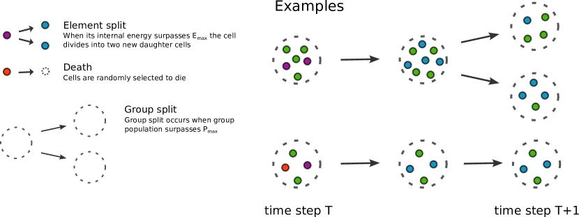
Figure 1: A graphical representation of the processes of group splitting, cell division and death.

The number of groups $N_{G}$ and their local population sizes $P_{i}$ ($i=1,...,N_{G}$) vary over time. A fundamental role is played by the influx of resource into the system (e.g. glucose) and how the resource is handled by the population, which in its turn can increase or shrink in size according to the amount of resource provided. In every time step, both individuals and groups can give rise to new individuals and groups, respectively. Each individual divides into two identical cells as soon as its internal energy storage $E_{ij}$ (group index, $i=1,...,N_{G}$, and individual index, $j=1,...,P_{i}$) surpasses the energy threshold $E_{\rm{max}}$. Each daughter cell inherits half of the energy of the parental cell. Groups have a threshold size $P_{\rm{max}}$, and whenever the number of individuals in a group reaches this limit, the group splits into two groups, with its members being evenly distributed between the two. The above described dynamics is also illustrated in Fig. 1. In addition, each individual dies at a constant probability $\nu$ per time step. The group death occurs when the number of individuals shrinks to zero.

In every time step, the amount of resource available to the population is constant and equal to $S$. We consider equipartition of resource among the groups and so the amount of resource per group is $S_{G}=S/N_{G}$. Note that the total number of groups $N_{G}$ is a dynamical number. We break the complete process of an individual gaining energy in two stages: first, individuals compete for the resource; second, the caught resource is ultimately converted into internal energy (ATP). The assumption of breaking down the process in two stages is in accordance with mechanistic models of cells [Weiße et al. 2015]: first, an enzyme transports the resource into the cell, and then a second set of enzymes metabolizes the resource into a generic form of energy, which includes ATP. The rates of import and of metabolism are distinct [Weiße et al. 2015].

Implementing the resource uptake

The resource is shared among the members of a group. As a strain type with rapid metabolism, $(D)$, has a higher rate of consumption, it seizes a larger portion of the resource available to the group compared with strains type $C$, characterized by a low consumption rate. The amount of resource per strain $D$ in a given group $i$ is estimated as

$$S^{i}_{D}(S_{G})=\frac{J^{S}_{D}(S_{G})}{J^{S}_{D}(S_{G})P^{i}_{D}+J^{S}_{C}(S_{G})P^{i}_{C}}\ S_{G},$$ (1)

where $P^{i}_{D}$ and $P^{i}_{C}$ are, respectively, the number of individuals for type $D$ and $C$ in group $i$, such that $P^{i}_{D}+P^{i}_{C}=P^{i}$ corresponds to the size of group $i$. The consumption rates for strain type $C$ and $D$, $J^{S}_{C}(S_{G})$ and $J^{S}_{D}(S_{G})$, are functions of $S_{G}$, the amount of resource per group. Similarly, the amount of resource per strain C is

$$S^{i}_{C}(S_{G})=\frac{J^{S}_{C}(S_{G})}{J^{S}_{D}(S_{G})P^{i}_{D}+J^{S}_{C}(S_{G})P^{i}_{C}}\ S_{G}.$$ (2)

Therefore, the total amount of resource for group $i$ is $S^{i}_{D}(S_{G})P^{i}_{D}+S^{i}_{C}(S_{G})P^{i}_{C}=S_{G}$ as declared above.

Implementing the conversion of resource into internal energy

The resource inside the cell is used to increment its internal energy $E_{ij}$, which is calculated as

$$\Delta E_{ij}=J^{ATP}_{C}(S^{i}_{C})\text{ or }\Delta E_{ij}=J^{ATP}_{D}(S^{i}_{D}),$$ (3)

depending on strain type, $C$ or $D$. The functions $J_{C}^{ATP}(S^{i}_{C})$ and $J_{D}^{ATP}(S^{i}_{D})$ represent how efficiently the resource ($S^{i}_{C}$ or $S^{i}_{D}$) is transformed into energy (ATP) for each individual type.

2.2 Simulation procedure

2.2.1 Statistical measurement

In the most probable scenario for the establishment of the efficient mode of metabolism, an alternative metabolic pathway arose by mutation in a pool of organisms making usage of resource inefficiently. For this sake, it is of practical importance to determine the probability that a single individual of type $C$ invades and ultimately dominates a population. The simulation initiates from an isogenic population of strains $D$ and let it evolve to a stationary regime. This step is required as the population dynamics and the resource availability determine the population size at the steady regime. For this reason the system is said to be self-organized. At this point, a single strain $C$ replaces a randomly chosen cell from the population. From this time on, the fate of the mutant type $C$ is observed, i.e., the simulation is tracked until the mutant gets lost or fixed.

The fixation probability is simply the fraction of independent runs at which the efficient strain gets fixed. Because the population size itself is an outcome of the dynamics of the model, it is rather desirable to present the outcomes in terms of the relative fixation probability, defined as fixation probability divided by $1/N_{\rm{st}}$. Here $N_{\rm{st}}$ stands for the population size of strains $D$ at the moment the efficient strain is introduced. Thus, $1/N_{\rm{st}}$ corresponds to the fixation probability of a mutant under neutral selection in a population of size $N_{\rm{st}}$. If the relative fixation probability is larger than one, the mutant type is said to be selected for, while a probability smaller than one means the strain is counter-selected.

2.2.2 Parametrization of the model

The rates of resource uptake and of conversion of food into energy appearing in Eqs. (1-2) are defined as

$$J^{S}_{C}(S_{G})=A_{C}\left(1-\exp(-\alpha{S_{G}})\right)$$ (4a)

$$J^{S}_{D}(S_{G})=A_{D}\left(1-\exp(-\alpha{S_{G}})\right)$$ (4b)

$$J^{ATP}_{C}(S_{i}^{C})=A^{ATP}_{C}\left(1-\exp(-\alpha^{ATP}_{C}{S_{C}^{i}})\right)$$ (4c)

$$J^{ATP}_{D}(S_{i}^{D})=A^{ATP}_{D}\left(1-\exp(-\alpha^{ATP}_{D}{S_{D}^{i}})\right).$$ (4d)

In common, all these functions display a sigmoidal shape, thus saturating for large values of $S$, similarly to Michaelis-Menten functions [Pfeiffer et al. 2001, Weiße et al. 2015]. The effect of the rates on the population dynamics is here extensively studied. For most of the parameters we will perform a sweep over the parameter space that covers the physically meaningful regions of interest. The maximum values for the rates are chosen in such way that the rate-yield trade-off exists. By definition, the efficient strain $C$ is the one that transforms resources into internal energy efficiently at the expense of the consumption rate, while strain $D$ metabolizes fast but at low yield. The parameters above follow some conditions:

• $A_{D}$ must be larger than $A_{C}$ ($A_{D}>A_{C}$), which assures that type $D$ always has a higher consumption rate for the same amount of resource. Note that the argument in the exponential function is exactly the same as in Eqs. 4a and 4b, and so it will have no influence on the dynamics. We just keep it for future generalisations. As naturally emerging in the forthcoming calculations, the relevant parameter is in fact the ratio between these two quantities, $\epsilon=A_{D}/A_{C}$.

• Another condition is $\Delta_{ATP}=\alpha^{ATP}_{D}/\alpha^{ATP}_{C}<1$. Once again, the ratio between the exponents in the functions (4)c and (4)d arises as a key quantity in the process. This condition warrants that strain $D$ is less effective than strain $C$ by generating energy from a given amount of resource, unless a very large amount of resource is gathered to be converted into energy. This is ensured when the ratio $\Gamma_{ATP}=A^{ATP}_{D}/A^{ATP}_{C}$ is larger than one, which allows a fast metabolic pathway to produce more energy in case they capture a much higher amount of resource than the efficient strain. This possibility is particularly important since it is known that many cells can work as a respiro-fermenting cells, concomitantly using the two alternative pathways of ATP production. Such respiro-fermentative metabolism is a typical mode of ATP production in unicellular eukaryotes like yeast [Frick and Schuster 2003, Otterstedt et al. 2004]. In such a situation, the yield of the whole process is reduced as the cell drives more resource to be metabolised inefficiently, a habitual behavior under the condition of plentiful resource. Of course, the situation $A^{ATP}_{D}<A^{ATP}_{C}$ can also be seen, but the opposite $A^{ATP}_{D}>A^{ATP}_{C}$ represents the worst scenario for the efficient strain, and if it can thrive in such case it will naturally be favored under less harsh conditions.

2.3 Social conflict

Besides settling down the constraints on the biological relevant parameter values, it is also important to find the parameter region at which the rate-yield trade-off in fact produces a tragedy of the commons [Hardin 1968]. The social conflict exists if in a pairwise competition for a common resource the strain with fast metabolism outcompetes the strain with high yield [Gudelj et al. 2007, Pfeiffer et al. 2001, MacLean 2008].

For a given resource influx rate $S^{*}$, the uptake of resource by strains $C$ and $D$ are, respectively,

$$S_{C}=\frac{J_{C}^{S}}{J_{C}^{S}+J_{D}^{S}}S^{*}$$ (5)

$$S_{D}=\frac{J_{D}^{S}}{J_{C}^{S}+J_{D}^{S}}S^{*}.$$ (6)

The ratio between $J_{D}^{ATP}$ and $J_{C}^{ATP}$ provides us the relative advantage of strain $D$ over strain $C$. From Eqs. (4) we obtain that

$$r=\frac{J_{D}^{ATP}}{J_{C}^{ATP}}=\Gamma_{ATP}\frac{1-\exp(-\alpha_{D}^{ATP}S_{D})}{1-\exp(-\alpha_{C}^{ATP}S_{C})}.$$ (7)

If this ratio is larger than one, the social conflict is held true. This reasoning will be employed to map the set of parameter values at which social conflict exists. As the ratio $r$ depends on the amount of resource, in order to delimit the social conflict region in a population of arbitrary size, we must use $S^{*}\simeq S/N$, instead of using $S$, the total resource influx rate. $N$ denotes the population size. Though, as observed from the simulations, the system evolves in such way that $S/N$ is always small at equilibrium. As we will see, the limit of small $S/N$ will prove to be useful in the forthcoming.

3 Results

We will start this section by presenting some analytical approximations for well-mixed populations. These calculations are useful in the sequel and serve as a guidance to determine the situations at which the simulations results match the theoretical prediction. They also help us to delimit the situations where phenomena driven by stochastic effects manifest, which are not captured by the analytical approach carried out here. As in the analytical approach structuring is not assumed, it will be particularly useful to demonstrate whether group structure can be a driving mechanism for the maintenance of the efficient strain.

3.1 Analytical results for well-mixed populations

3.1.1 Equilibrium size of a population of strains with fast metabolism

Let us propose a discrete-time model for a well-mixed population with only cells of type $D$. More generally, the population size in time step $t+1$ can be written as

$$n(t+1)=n(t)+g(n(t),S)\,n(t)-\nu\,n(t),$$ (8)

where the function $g(n(t),S)$ denotes the growth rate of strain $D$, which depends on the population size as well as on the resource influx rate, $S$. The death rate is denoted by $\nu$ (as a mathematical guide for the analytical development to be done, we suggest as a reference [Otto and Day 2007]). In the above equation, it is implicitly assumed that $g(n(t),S)$ is proportional to the amount of resource captured by the consumer. The conversion of resource into energy (directly translated as growth rate) occurs into two steps: uptake of resource, and its posterior conversion into energy. As there is only one type of strain, the amount of resource per individual at time $t$ is just $S/n(t)$. Following Eq. (4d), the growth rate is equivalent to $g(n(t),S)=a_{D}\left[1-\exp(-\alpha_{D}^{ATP}S/n(t))\right]$, where $a_{D}=A_{D}^{ATP}/E_{\rm{max}}$, which is a necessary rescaling because individuals only replicate if their internal energies surpass the threshold $E_{\rm{max}}$. Plugging this expression into Eq. (8) we get

$$n(t+1)=n(t)+a_{D}\left[1-\exp(-\alpha_{D}^{ATP}S/n(t))\right]n(t)-\nu n(t).$$ (9)

The system is under equilibrium when $n(t+1)=n(t)=\hat{n}$ and has two equilibrium solutions, $\hat{n}=0$ and $\hat{n}=-\frac{\alpha_{D}^{ATP}S}{\ln(1-\nu/a_{D})}$. Note that the second solution is only meaningful if $\nu<a_{D}$.

3.1.2 Stability Analysis

Next we analyze the local stability of the two equilibrium solutions. By writing the dynamics of the discrete-time model like $n(t+1)=f(n(t))$, a solution, $n=\hat{n}$, is said to be stable when $-1<\lambda<1$, where $\left.\lambda=\frac{df}{dn}\right|_{n=\hat{n}}$. Note that the derivative of $f(n(t))$ with respect to $n$ must be evaluated at the equilibrium. A value of $\left|\lambda\right|<1$ warrants that any small perturbation from the equilibrium solution will be damped, bringing the system back to equilibrium. Whenever $\left|\lambda\right|>1$, any disturbance drives the system away from the equilibrium point.

For the first equilibrium, $\hat{n}=0$, $\lambda$ is evaluated as $\left.\lambda=\frac{df}{dn}\right|_{\hat{n}=0}=1-\nu+a_{D}$, and so the solution is stable when $\nu>a_{D}$, i.e. $\nu E_{\rm{max}}>A_{D}^{ATP}$. On the other hand, the second equilibrium, $\hat{n}=-\frac{\alpha^{ATP}S}{\ln(1-\nu/a_{D})}$, provides $\left.\lambda=\frac{df}{dn}\right|_{\hat{n}=-\frac{\alpha^{ATP}_{D}\,S}{\ln(1-\nu/a_{D})}}=1+a_{D}(1-\nu/a_{D})\ln(1-\nu/a_{D})$. Because $\nu<a_{D}$ in the range of validity of the solution, the logarithm is always negative, meaning $\lambda<1$. Therefore, the second solution is always stable in the range it is valid.

3.2 Evolutionary Invasion Analysis

3.2.1 Invasion by the efficient strain

A further step of our analytical calculation is to check under which conditions a population of strain with rapid growth can be invaded by a mutant that uses the resource more efficiently. The simulations depart from an isogenic population of strain $D$, and after a stationary state a single type $C$ individual is introduced. The dynamics in terms of the number of individuals of strains $D$ and $C$ over time, $n_{D}$ and $n_{C}$ respectively, is now determined by the following set of equations:

$$n_{D}(t+1) =n_{D}(t)\{1+a_{D}\left[1-e^{-\alpha_{D}^{ATP}\frac{J_{D}^{S}S}{J_{D}^{S}n_{D}+J_{C}^{S}n_{C}}}\right]-\nu\}$$ (10)

$$n_{C}(t+1) =n_{C}(t)\{1+a_{C}\left[1-e^{-\alpha_{C}^{ATP}\frac{J_{C}^{S}S}{J_{D}^{S}n_{D}+J_{C}^{S}n_{C}}}\right]-\nu\},$$ (11)

and now $a_{C}=A_{C}^{ATP}/E_{\rm{max}}$. It is important to point out that since there are two distinct strains, the amount of resource captured per individual is no longer $S/n$ but obeys the resource partition as calculated by Eqs. 1$\&$2. The dynamics is driven by a density dependent growth rate. One possible equilibrium of the above system is

$$\hat{n}_{D}=-\frac{\alpha_{D}^{ATP}S}{\ln(1-\nu/a_{D})}~{}~{}~{}~{}~{}~{}~{}~{}\mbox{and}~{}~{}~{}~{}~{}~{}~{}~{}\hat{n}_{C}=0.$$ (12)

This equilibrium corresponds to the nonzero equilibrium of the resident population of strain $D$, as shown in 3.1.1.

Next we analyse the stability conditions of this equilibrium under the invasion of a small quantity of efficient strains. For multiple-variable models, the local stability of the equilibrium solutions is found by looking at the eigenvalues of the Jacobian matrix of the system, see details in the Supporting Information.

After determining the eigenvalues and setting the conditions for stability (please see Supporting Information), it is possible to disclose a relationship delimiting the parameter region at which the efficient strain can invade the resident population of type $D$ cells. For fixed $A_{C}^{ATP}$ and variable $A_{D}^{ATP}$ we find that

$$\Gamma_{ATP}=\frac{\nu/a_{C}}{1-(1-\nu/a_{C})^{\Delta_{ATP}\epsilon}},$$ (13)

where $\Delta_{ATP}=\frac{\alpha_{D}^{ATP}}{\alpha_{C}^{ATP}}$ and $\epsilon=\frac{A_{D}}{A_{C}}$, as previously defined. Eq.(13) is used for the comparison with the isocline $P_{fix}=1$, fixation probability equal to one, obtained from simulations. Therefore, our finding shows that the solution, eq.(12), is stable against invasion above the curve (13), while the strain $C$ can succeed to invade in the parameter space under the curve.

3.2.2 Invasion by the inefficient strain

Now the opposite situation is considered — the conditions under which a mutant with rapid metabolism (type $D$) can invade a population dominated by cells of type $C$. The calculations are straightforward as calculations are similar as in Sec.3.2.1. As the resident population is initially composed of cells type $C$ only, its size at equilibrium is $n_{c}=\hat{n}_{C}=-\frac{\alpha_{C}^{ATP}S}{\ln(1-\nu/a_{C})}$, and $a_{C}=A_{C}^{ATP}/E_{\rm{max}}$.

The Jacobian matrix is now evaluated at

$$\hat{n}_{C}=-\frac{\alpha_{C}^{ATP}S}{\ln(1-\nu/a_{C})}~{}~{}~{}~{}~{}~{}~{}~{}\mbox{and}~{}~{}~{}~{}~{}~{}~{}~{}\hat{n}_{D}=0$$ (14)

as the strain $D$ is assumed to be rare. Likewise, a relation between $\Gamma_{ATP}$ and $\Delta_{ATP}$ is obtained, and the curve now delimits the parameter region at which the efficient strain is stable against the invasion by the inefficient strain. It is found that

$$\Gamma_{ATP}=\frac{\nu/a_{C}}{1-(1-\nu/a_{C})^{\Delta_{ATP}\epsilon}},$$ (15)

which is exactly equal to Eq.(13). However, now the solution, eq. (14), is stable under the curve. Thus, we conclude that the parameter region $\Gamma_{ATP}$ versus $\Delta_{ATP}$, where the efficient strain is evolutionary stable against the invasion by the selfish strain $D$, coincides with the region at which it can, while rare, invade an isogenic population of type $D$ individuals.

3.3 Simulation Results

In this section we present the simulation results of the evolutionary invasion analysis. In Supporting Information we provide simulation results and present the plots of the population size of isogenic population of strain $D$ at equilibrium. This is critical as the population size determines the strength of stochasticity on the dynamics of the system.

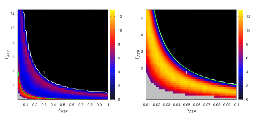
Figure 2: Fixation probability. In the plot the fixation probability is shown in terms of $\Gamma_{ATP}=A^{ATP}_{D}/A^{ATP}_{C}$ and $\Delta_{ATP}=\alpha^{ATP}_{D}/\alpha^{ATP}_{C}$. Left panel: structured populations, right panel: homogeneous populations. The white thick lines denote the isocline where the fixation probability of a single cooperator is the same as the fixation probability of a random individual under neutral selection. Above the isocline the cooperative strategy is counter-selected (dark region), whereas under the line it is selected for. Yet, the green line corresponds to the line delimiting the social conflict regime, obtained by making $r=1$ in eq. 7. This line overlaps the lines given in eqs (13) and (15). Once again, the grey region denotes that the defector population goes to extinction before the cooperator is introduced. The other parameter values are influx rate of resource $S=25$, death rate $\nu=0.01$, group carrying capacity $P_{\rm{max}}=10$, internal energy for splitting $E_{\rm{max}}=10$, and $A_{D}=10$. The data points corresponds to $40$ distinct populations and for each population $10,000$ independent runs were performed.

3.3.1 The relative fixation probability of a single individual of the efficient strain

From the heat map in Fig. 2 we observe how the fixation probability is influenced by the ratios, $\Gamma_{ATP}=A^{ATP}_{D}/A^{ATP}_{C}$ and $\Delta_{ATP}=\alpha^{ATP}_{D}/\alpha^{ATP}_{C}$. The ratio $\epsilon=A_{D}/A_{C}$ is set at $10$, which is a typical value, as empirically measured in populations of S. cerevisiae [Otterstedt et al. 2004]. Making the comparison with well-mixed populations, over a broader domain of the parameter space the efficient strain is selected for in the structured populations. When $\Delta_{ATP}$ is already close to one, meaning that the yield of strain $D$ is almost equivalent to strain $C$, it still persists a domain at which efficient strain is favored. The domain at which the efficient strain is favored in well-mixed populations is considerably restricted in comparison to structured populations. For instance, around $\Delta_{ATP}=0.1$ the efficient strain is already unlikely to invade and to fixate.

The curves corresponding to eqs. (13) and (15) are represented by the green line in the left and the right panels of Fig. 2. The region below the green line portrays the domain at which the efficient strain can invade and replace a population of individuals type $D$. Of course, the outcome of the dynamics is not deterministic, but it evidences a selective advantage for strain $C$ . The white line is the isocline $P_{fix}=1$ (fixation probability is equal to one). The line setting out the onset of the social conflict, corresponding to $r=1$ in eq. (7), is also plotted. In well-mixed populations (right panel of Fig. 2) the social conflict line ($r=1$) overlaps with the green line, eqs. (13) and (15), and thence it is not perceivable in the plot. Indeed, in the limit $S/N$ small, which always holds when $\nu/a_{D}$ is also small (see Eq. (12)), the two curves are essentially the same and become $\Gamma_{ATP}=\frac{1}{\Delta_{ATP}\epsilon}$. This observation leads us to conclude that in well-mixed populations the efficient strain is an effective intruder only in the domain there is no dilemma.

On the other hand, in structured populations the efficient strain is selectively advantageous over a much larger set of the parameter space. The realm of the high yield strain goes further beyond the line setting out the social conflict. The isocline $P_{fix}=1$ is considerably shifted to the right. The region between the social conflict line (green line) and the isocline $P_{fix}=1$ is of special interest, since it shows the prominent role of structuring — more specifically kin-selection — on promoting the fixation and maintenance of the strain exploiting the resource efficiently.

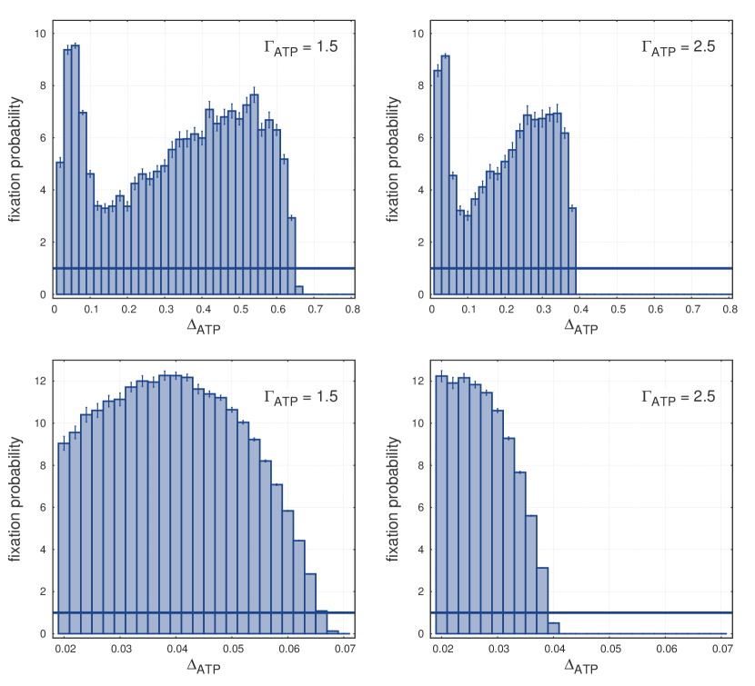
Figure 3: Fixation probability as a function of $\Delta_{ATP}$ for fixed values of $\Gamma_{ATP}$. In top panel we exhibit the simulation outcomes for structured populations whereas in the bottom panels for homogeneous populations. The data points correspond to $40$ distinct populations and for each population $100,000$ independent runs were performed. The parameter values are $S=25$, $\nu=0.01$, $P_{\rm{max}}=10$, $E_{\rm{max}}=10$, $A_{D}=10$, and $A_{C}=1$.

Looking at the heat map, it is noticeable that there exists a non-straightforward relationship between $\Delta_{ATP}$ and $\Gamma_{ATP}$. At fixed $\Gamma_{ATP}$ the relative fixation probability approaches a two-humped function of $\Delta_{ATP}$, being maximised at low and intermediate values of $\Delta_{ATP}$ (see Fig. 3). In the panels, $\Gamma_{ATP}$ is kept constant while $\Delta_{ATP}$ varies. Well-mixed populations (lower panels) display a smoother scenario and the relative fixation probability is now an one-humped function of $\Delta_{ATP}$. The point, at which the relative probability is maximised, depends on $\Gamma_{ATP}$, being shifted towards higher values of the ratio $\Delta_{ATP}$ as $\Gamma_{ATP}$ decreases. In well-mixed populations the selective advantage of strain $C$ over strain $D$ is confined to the region where there is no dilemma. Yet, in structured populations the range of $\Delta_{ATP}$ in the plot embodies three distinct regions: the region at which there is no dilemma, a second region where the dilemma exists and the efficient strain has a selective advantage, and a last one at which the dilemma still holds but the efficient strain is no longer able to persist. The first peak occurs at small $\Delta_{ATP}$ as observed in well-mixed population, but now there is a second peak that lies at the range of intermediate values of $\Delta_{ATP}$. This latter peak has no counterpart in a scenario of well-mixing, as it is promoted by kin-selection.

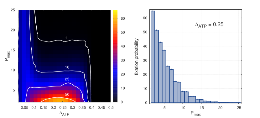
Figure 4: The strength of stochasticity. The left panel shows the fixation probability in terms of the carrying capacity $P_{\rm{max}}$ and the ratio $\Delta_{ATP}$. The right panel represents how the fixation probability changes with $P_{\rm{max}}$ in a given $\Delta_{ATP}$. The thick white lines correspond to isoclines. The parameter values are $S=25$, $\nu=0.01$, $E_{\rm{max}}=10$, $A_{D}=5$, and $\Gamma_{ATP}=2.5$. The data points correspond to $40$ distinct populations and for each population $10,000$ ($100,000$) independent runs were performed in left panel (right panel).

Next we study how the relative fixation probability changes with the group carrying capacity, $P_{\rm{max}}$. This analysis enables to assess the strength of stochasticity and kin-selection on the population dynamics. Smaller group sizes entail higher relatedness among individuals in the same group. Previous studies have claimed that in multilevel selection the likelihood of invasion and posterior fixation of cooperative traits is particularly enhanced for small group sizes [Traulsen and Nowak 2006], evidencing the importance of stochasticity in the dynamics [Nowak et al. 2004]. Similar behaviour was observed in a resource-based model of pairwise interactions within the multilevel selection framework [Ferreira and Campos 2013]. The contour map in the left panel of Fig. 4 displays the relative fixation probability for different values of $P_{\rm{max}}$ and different values of $\Delta_{ATP}$. The lighter colours in the bottom of the plot evince that the efficient strain $C$ is significantly favored as smaller group size is considered. For extremely small group sizes, like $P_{\rm{max}}=5$, the fixation probability varies enormously with the ratio $\Delta_{ATP}$, being maximised at intermediate values. In such small groups, the fixation probability can be sixty-fold higher than fixation probability of a neutral trait. At large values of $P_{\rm{max}}$, instead of a pronounced change with $\Delta_{ATP}$, the probability is roughly constant at a broad interval range of $\Delta_{ATP}$, as inferred from the isoclines. Of particular interest is the isocline delimiting the onset of the phase at which the efficient strain is favored. From the isocline $P_{fix}=1$ one deduces that for $\Delta_{ATP}$ varying between $0.1$ and $0.4$ there is a well-defined critical value for the group carrying capacity, which is about $P_{\rm{max,c}}\simeq 17$, beyond which the efficient strain becomes counter-selected. Though, as the efficiency of the strain $D$ is further reduced (small $\Delta_{ATP}$), the critical group size $P_{\rm{max,c}}$ soars again. For the sake of completeness, the right panel of Fig. 4 shows that the relative fixation probability is a well-behaved monotonic decreasing function of $P_{\rm{max}}$ under fixed $\Delta_{ATP}$.

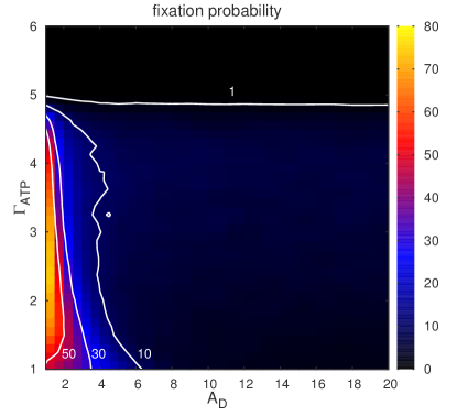
Figure 5: The effect of the consumption rate. Heat map of the fixation probability in terms of the ratio $\Gamma_{ATP}$ and the consumption rate of defectors $A_{D}$. The parameter values are $S=25$, $\nu=0.01$, $P_{\rm{max}}=10$, $E_{\rm{max}}=10$, and $\Delta_{ATP}=0.2$. The thick white lines correspond to isoclines. The data points correspond to an average over $10$ distinct populations and for each population $10,000$ independent runs.

How the consumption rate affects the fate of the efficient strain with a low frequency is studied in Fig. 5. A contour plot in terms of $\Gamma_{ATP}$ and $A_{D}$ is presented. The consumption rate is naturally a relevant part in the process since the amount of energy added to the individual’s internal energy is bounded to the amount of resource caught, which by its turn also influences other individuals’ performance due to competition. The selfish strategy enjoys a twofold benefit when both $A_{D}$ and $\Gamma_{ATP}$ are kept high. First in the competition for the resource, as a high $A_{D}$ means a big advantage in the resource uptake, and subsequently in process of conversion of resource into energy which is determined by its efficiency, see Fig. 5. As illustrated in the plot, the left right corner is dark-coloured meaning that the efficient strain is clearly counter-selected. $\Gamma_{ATP}$ has a more influential role than $A_{D}$. At $A_{D}\simeq 5$, a further increase of the variable does not lead to any substantial variation of the fixation probability.

3.4 Enabling migration between groups

As learned from the previous discussions, a way to reduce the strength of kin-selection and thus allowing a less favorable environment for the promotion of efficient usage of resource is to increase the group carrying capacity $P_{max}$. An alternative manner to change the strength of kin-selection is presented. Now we allow individuals to migrate: at each generation every individual has a probability $m$ to leave its original group and move to a randomly chosen group in the population. This is known as the island model of stochastic migration [Wright 1943]. By allowing migration to occur, one can tune the level of relatedness among individuals, which tends to decrease as the migration rate is increased.

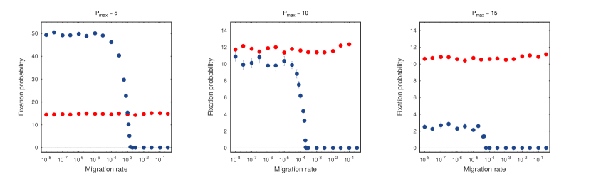
Figure 6: Effect of migration on the fixation probability. The fixation probability is plotted as a function of the migration rate $m$ for three distinct values of carrying capacity $P_{\rm{max}}$. The parameter values are $S=25$, $\nu=0.01$, $E_{\rm{max}}=10$, $A_{D}=10$, $A_{C}=1$, $\Gamma_{ATP}=1.5$ and $\Delta_{ATP}=0.5$ (blue points) and $\Delta_{ATP}=0.04$ (red points).

The effect of the migration rate on the fixation probability can be seen in Fig. 6. Different situations are considered in the face of our previous knowledge about the system. Distinct values of $\Delta_{ATP}$ and of carrying capacity $P_{\rm{max}}$ are considered. At $\Delta_{ATP}=0.5$ (blue points) the efficient strain is selected against in well-mixed populations but not in structured populations. At $\Delta_{ATP}=0.04$ (red points) the efficient strain is favored in both scenarios. In the latter situation, migration does not affect the outcome and the fixation probability is invariant. Helpful information about the role of migration is gathered from the analysis of the case $\Delta_{ATP}=0.5$. Starting from small migration rates, which means the groups are more isolated and relatedness is high, the fixation probability is nearly the same over a wide range of migration, and then sharply goes to zero as the rate of migration is further augmented, signifying less isolation. The first plateau coincides with the value of the fixation probability in our structured population model, while after the transition the situation resembles well-mixed populations at which the efficient strain can no longer thrive.

4 Discussion

We have studied the evolutionary dynamics of a population with two strains under a trade-off between rate and yield. The two strains with distinct metabolic pathways compete under a scenario of limited resource. This problem has long been debated within the framework of evolution of cooperation, as the strain that uses resource efficiently is described as a cooperator, while the strain with high uptake rate, at the expense and degradation of its own environment, is said to display a defecting behavior [Pfeiffer et al. 2001, Kreft and Bonhoeffer 2005]. The trade-off between high rate and yield occurs due to biophysical restraints. Experimental results show a clear negative correlation between resource uptake and efficiency of conversion of resource into energy [Pfeiffer et al. 2001, Kreft 2004, Meyer et al. 2015]. The existence of such trade-offs in heterotrophic microorganisms, like bacteria and yeast, and the fact that the efficient manipulation of resource was made possible with the appearance of the metabolic pathway that makes use of oxygen, the so-called respirers, have motivated a large body of studies. A clear motivation is the issue related to the major transition from single cells towards multicellular forms of life [Pfeiffer and Bonhoeffer 2003, Aledo 2008]. Multicellularity can thus be thought as the integration of smaller units to build up a more complex machinery.

Kin selection as one possible driving force promoting the units that make efficient handling of resource is effective when relatedness among individuals is relatively high such that the cost of the cooperative act can be balanced. A natural way to enhance relatedness is to increase cohesion or the level of clustering in the population. Here we proposed an explicit resource-based model in which competing metabolic strategies are assumed. We studied the conditions under which the cooperative strain with high yield metabolism can invade and outcompete a resident population of selfish strains. By investigating structured and well-mixed populations we aim to understand whether the existence of group structure is a required condition for the maintenance of efficient metabolism pathways.

We showed that in well-mixed populations the efficient strain is only viable in a subset of the parameter space corresponding to the region where there is no social conflict. In other words, the efficient strain can only invade a population of inefficient strains when it is rare, under the condition it is already a strong competitor in a pairwise competition with its opponent. The lines delimiting the social conflict region and the isocline $P_{fix}=1$ overlap. These lines also delimit the region of stability of the two competing metabolic strategies. Together, these results suggest that a complete mixing of cells creates an unfavorable scenario for the appearance and subsequent maintenance of an efficient mode of metabolism.

On the other hand, in structured populations a more favorable scenario is presented. Over a broad domain of the parameter space, which goes further beyond the boundaries settled down by the social conflict and the invasion analysis, the efficient strain is selected for. This result highlights the role of structuring, and more specifically kin selection, in promoting the efficient mode of metabolism. In a population which assumes complete mixing of individuals, relatedness is expected to be low, while in structured populations relatedness is expected to be relatively higher. This is corroborated when we studied the effect of migration on the dynamics of fixation of the efficient strain. As migration is reduced, isolation increases, and so does the strength of kin selection. An abrupt soaring of the fixation probability of the efficient strain was observed. Although local competition among relatives may increase in structured populations [Taylor 1992, Taylor 1992, West et al. 2002], it does not mitigate the benefits of kin-selection in the model. More evidence of this finding is obtained by checking the dependence of the fixation probability on the carrying capacity $P_{max}$, whereby it is demonstrated that the efficient strain faces an even more favorable environment when smaller groups are assumed.

So one question remains: which mechanism relieves the effect of increased competition in small groups thus turning kin-selection an effective evolutionary force? Local competition for resource is attenuated in the structured populations as groups are elastic and their sizes can vary between fission events. This is consistent with previous findings [West et al. 2002, Kümmerli et al. 2009]. Although a larger group means less resource available per individual, there is no competition for space. Once one individual reproduces it does not necessarily lead to the removal of any interactant. Additionally, a group containing more efficient individuals has as advantage, as a larger amount of resource will be available and the net amount of energy converted in the process can be larger. This allows the group to reach the carrying capacity $P_{max}$ faster. The fact that overlapping generations increase relatedness also contributes to enhance the chance of the efficient trait [West et al. 2002]. The third mechanism is the process of group split, which produces a two-fold benefit: first by reducing local competition because after division the number of cells per group drops; second, if the number of efficient cells that occupy a given group increases, so does the chance that a new-born group is only filled by efficient strains, thus helping to perpetuate the trait. In summary, three premises of the model — group expansion, overlapping generations and group split — contribute to attenuate local competition thus allowing a net benefit effect of kin selection.

The observation of a critical value of $P_{\rm{max}}$ imposes a threshold for kin selection to act as an effective force. Larger group sizes entail smaller relatedness in such way that Hamilton’s rule $bc>r$ is no longer followed. The group split is a key premise of the model. In a recent work, Ratcliff et al. designed an experiment to understand the evolution of complex multicellular organisms from unicellular ancestors [Ratcliff et al. 2012]. In the experiment, a population of yeast (S. cerevisiae) was artificially selected for multicellularity by growing in nutrient-rich medium. Serial transfers of the bottom fraction of the liquid were performed, and cells collected together with the liquid formed the next generation. After few transfers, they already observed that populations were dominated by snowflake-shaped multicellular clusters. Their witness of the occurrence of cluster reproduction is a basic premise to settle down life in its multicellular form. The authors ascertained that the daughter clusters were produced as multicellular propagules rather than mass dissolution of parental clusters. They also observed the existence of a threshold for the minimum size of daughter clusters [Ratcliff et al. 2012]. In our viewpoint, the findings in the experiment of Ratcliff et al. are in line with the assumptions of the group dynamics of the proposed model in the current work.

As conjectured, the first step in the evolutionary transition from single-celled to multicellular organisms most likely involved the evolution of undifferentiated multicellularity [Pfeiffer and Bonhoeffer 2003]. Our results show that it is very unlikely that the efficient mode of ATP production has arisen and has become widespread in a scenario of global interaction and competition (complete mixing). Once there are efficient strains arising through mutation, the maintenance of those strains in a well-mixed population would be very improbable as they could be easily invaded by strains with higher growth rate in spite of its low efficient metabolism. Alternatively, the appearance and subsequent growth of efficient strains in frequency must come together with the emergence of a mechanism that prevents dividing cells from complete separation enabling clusters through parent-offspring adhesion [Ratcliff et al. 2012].

Supporting Information

Appendix A The Jacobian matrix

Here we calculate the eigenvalues of the Jacobian matrix of the discrete model. If the absolute values of the eigenvalues are smaller than one then the solution in Section 3.2.1 is stable. If we write the set of equations (10) of our two-variable model as $n_{D}(t+1)=f_{D}(n_{D},n_{C})$ and $n_{C}(t+1)=f_{C}(n_{D},n_{C})$, the Jacobian matrix is defined as

$$J=\left(\begin{array}[]{cc}\frac{\partial f_{D}}{\partial n_{D}}&\frac{\partial f_{D}}{\partial n_{C}}\\ \frac{\partial f_{C}}{\partial n_{D}}&\frac{\partial f_{C}}{\partial n_{C}}\end{array}\right).$$

The Jacobian matrix must be evaluated at the equilibrium of interest, i.e. $\hat{n}_{C}=0$ and $\hat{n}_{D}=-\frac{\alpha_{D}^{ATP}S}{\ln(1-\nu/a_{D})}$. After some algebra, the coefficients of the matrix at the equilibrium of interest are determined

$$J=\left(\begin{array}[]{cc}1+a_{D}(1-\nu/a_{D})\ln(1-\nu/a_{D})&\frac{a_{D}}{\epsilon}(1-\nu/a_{D})\ln(1-\nu/a_{D})\\ 0&1-\nu+a_{C}\left[1-(1-\nu/a)^{\frac{1}{\Delta_{ATP}\epsilon}}\right]\end{array}\right),$$

where $\Delta_{ATP}=\frac{\alpha_{D}^{ATP}}{\alpha_{C}^{ATP}}$ and $\epsilon=\frac{A_{D}}{A_{C}}$. The above matrix is upper diagonal which means that the eigenvalues of the Jacobian are simply the diagonal coefficients. Because $\nu<a_{D}$ for the referred equilibrium, the element $J_{11}$ is always smaller than one and positive regardless the values of $\nu$ and $a_{D}$. Note that the logarithmic term is always negative. Therefore, the stability of the solution is uniquely settled by the element $J_{22}$. Of particular interest is the point at which the equilibrium becomes unstable which occurs when $J_{22}$ equals one. Making $J_{22}$ equal to one a relation between $\Gamma_{ATP}$ and $\Delta_{ATP}$ is obtained.

The same analysis is done in Section 3.2.2, but instead the solution $\hat{n}_{D}=0$ and $\hat{n}_{C}=-\frac{\alpha_{C}^{ATP}S}{\ln(1-\nu/a_{C})}$ is considered.

Appendix B Coexistence solution

The system of equations (10) also admits a solution where the two strains coexist. By rearranging the set of equations we verify that the coexistence solution obeys the following set of equations:

$$n_{D}\epsilon+n_{C}=-\frac{\alpha_{D}^{ATP}S\epsilon}{\ln(1-\nu/a_{D})}$$ (SI 1)

$$n_{D}\epsilon+n_{C}=-\frac{\alpha_{C}^{ATP}S}{\ln(1-\nu/a_{C})},$$ (SI 2)

showing that there is an indeterminacy, and the coexistence solution only exists when $\Delta_{ATP}=\frac{1}{\epsilon}\frac{\ln(1-\nu/a_{D})}{\ln(1-\nu/a_{C})}$. Actually Eq. (SI 1) describes a family of solutions. Of course, the range of values at which $n_{D}$ and $n_{C}$ are meaningful are $n_{C}\in[0,\mathcal{N}]$ and $n_{D}\in[0,\mathcal{N}]$, where $\mathcal{N}=-\frac{\alpha_{C}^{ATP}S}{\ln(1-\nu/a_{C})}$ with the constraint that $n_{D}\epsilon+n_{C}=-\frac{\alpha_{C}^{ATP}S}{\ln(1-\nu/a_{C})}$. Note that when $n_{C}=0$ we recover the solution $n_{D}=-\frac{\alpha_{D}^{ATP}S}{\ln(1-\nu/a_{D})}$, whereas if $n_{D}=0$ we recover the solution $n_{C}=-\frac{\alpha_{C}^{ATP}S}{\ln(1-\nu/a_{C})}$. By determining the Jacobian of the system at equilibrium and hence calculating its corresponding eigenvalues we check whether the coexistence solution is stable or not. With the help of mathematica, we performed a numerical computation of the eigenvalues for different set of parameters by varying all the range of acceptable values of $n_{D}$ (since $n_{C}$ is written as a function of $n_{D}$). As expected in this situation, one of the eigenvalues is equal to one, which means that any disturbance in the same direction as the line drives the system to the new values of $(n_{D},n_{C})$. This is called marginal stability as found in a simple predator-prey model studied by Lotka and Volterra [Parker and Kamenev 2010]. The stability of the family of solutions will be dictated by the second eigenvalue. For the set of parameter values used in our simulations the second eigenvalue is slightly smaller than one, meaning that any transverse disturbance is damped by the system, thus warranting stability of the family of solution in Eq. (SI 1). It is important to highlight that the coexistence solution only holds for $\Delta_{ATP}=\frac{1}{\epsilon}\frac{\ln(1-\nu/a_{D})}{\ln(1-\nu/a_{C})}$, which describes a line in the diagram $\Delta_{ATP}$ versus $\Gamma_{ATP}$.

In addition, from Eq. (10) we also notice that $\hat{n}_{D}=0$ and $\hat{n}_{C}=0$ are also equilibrium solutions, where both types go extinct. The solution is only stable when $\nu>a_{D}$ and $\nu>a_{C}$.

The coexistence of the two strains can not be observed in the simulations as the family of solutions embodies the absorbing states $n_{C}=0$ and $n_{D}=0$. As stochasticity plays a key role in finite populations, in a finite time the system will eventually reach one of these boundaries. Since we always start from $n_{C}=1$, the system will probably evolve to $n_{C}=0$ in a short time.

Appendix C Population size at equilibrium

Here we show how the stationary population size of individuals type $D$ (before introducing a single strain $C$), $N_{\rm{st}}$, depends on the set of parameters. From this we gain some insight about the strength of stochasticity. As intuitively expected, a linear relation between population size and the influx of resource into the system is observed (data not shown). The linearity is not followed when studying the dependence of the population size on the other parameters.

In Figure S1 we show the population size in terms of $\Gamma_{ATP}=A^{ATP}_{D}/A^{ATP}_{C}$ and $\Delta_{ATP}=\alpha^{ATP}_{D}/\alpha^{ATP}_{C}$, for both structured (left panel) and panmictic populations (middle panel). The values of $\Gamma_{ATP}$ and $\Delta_{ATP}$ are varied by keeping $A^{ATP}_{C}=2$ and $\alpha^{ATP}_{C}=0.5$ and changing $A^{ATP}_{D}$ and $\alpha^{ATP}_{D}$, respectively. The range of values of $\Gamma_{ATP}$ and $\Delta_{ATP}$ are, as argued before, those that are meaningful to the problem here addressed. Please note that a logarithmic scale is adopted for the color gradation in Fig. S1. The range of $\Delta_{ATP}=\alpha^{ATP}_{D}/\alpha^{ATP}_{C}$ in which population size is shown for the well-mixed populations is much smaller than the range displayed for structured population. Outside of this range the population already falls in the regime where the efficient strain is counter-selected - as can be seen in Fig. 2 (Main Text). The right panel of Fig. S1 shows the equilibrium solution for the discrete-time model of a well-mixed population, given by $\hat{n}=-\frac{\alpha_{D}^{ATP}S}{\ln(1-\nu\frac{E_{max}}{A_{D}^{ATP}})}$, as derived in Section 3.1.1. The grey region denotes the extinction of the population, where the above solution becomes unstable, while the solution $\hat{n}=0$ becomes stable. The plot evinces a very good agreement between the theoretical prediction and simulations. The simulation results for a well-mixed population display a larger grey area in comparison to the theoretical prediction, which owes to stochastic effects, which are not captured by the time-discrete model. In the right panel, the population size is too small — around five or less individuals — being prone to extinction.

Especially, in structured populations the stationary population size $N_{\rm{st}}$ of a pure population of strain $D$ can vary from less than $100$ individuals (small $\Gamma_{ATP}$ and $\Delta_{ATP}$) to nearly $5,000$ individuals (large $\Gamma_{ATP}$ and $\Delta_{ATP}$). The wide range of the population size at equilibrium explains why we should adopt a relative measurement of fixation probability since the strength of drift, namely $1/N_{\rm{st}}$, is variable under the change of the parameter values.

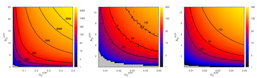
Figure S1: Stationary population size of defectors. The figure is a heat map of the population size of defectors (just before the introduction of a single cooperator) in terms of $A^{ATP}_{D}$ and $\alpha^{ATP}_{D}$. Left panel: simulation results for structured populations, middle panel: simulation results for well-mixed populations and right panel: theoretical prediction, $n_{D}=-\frac{\alpha_{D}^{ATP}S}{\ln(1-\nu E_{\rm{max}}/A_{D}^{ATP})}$. The other parameter values are influx rate of resource $S=25$, death rate $\nu=0.01$, group carrying capacity $P_{\rm{max}}=10$, internal energy for one individual to split to two individuals $E_{\rm{max}}=10$, and $A_{D}=10$. The simulation data points correspond to $40$ distinct populations and for each population $10,000$ independent runs were performed. The black lines denote isoclines, along which the population size is a constant (corresponding values indicated). The grey region denotes a region where the defector population is not sustainable and goes to extinction (before inserting the cooperator).

References

- Aledo 2008 Aledo, J. C. (2008). An early and anaerobic scenario for the transition to undifferentiated multicellularity. Journal of molecular evolution 67(2), 145–153.
- Aledo et al. 2007 Aledo, J. C., J. A. Pérez-Claros, and A. E. Del Valle (2007). Switching between cooperation and competition in the use of extracellular glucose. Journal of molecular evolution 65, 328–339.
- Claessen et al. 2014 Claessen, D., D. E. Rozen, O. P. Kuipers, L. Søgaard-Andersen, and G. P. van Wezel (2014). Bacterial solutions to multicellularity: a tale of biofilms, filaments and fruiting bodies. Nature Reviews Microbiology 12(2), 115–124.
- El Mouden and Gardner 2008 El Mouden, C. and A. Gardner (2008). Nice natives and mean migrants: the evolution of dispersal-dependent social behaviour in viscous populations. Journal of evolutionary biology 21(6), 1480–1491.
- Ferreira and Campos 2013 Ferreira, F. F. and P. R. A. Campos (2013). Multilevel selection in a resource-based model. Phys. Rev. E 88, 014101.
- Frick and Schuster 2003 Frick, T. and S. Schuster (2003). An example of the prisoner’s dilemma in biochemistry. Naturwissenschaften 90(7), 327–331.
- Gardner and West 2006 Gardner, A. and S. West (2006). Demography, altruism, and the benefits of budding. Journal of evolutionary biology 19(5), 1707–1716.
- Griffin et al. 2004 Griffin, A. S., S. A. West, and A. Buckling (2004). Cooperation and competition in pathogenic bacteria. Nature 430(7003), 1024–1027.
- Gudelj et al. 2007 Gudelj, I., R. Beardmore, S. Arkin, and R. MacLean (2007). Constraints on microbial metabolism drive evolutionary diversification in homogeneous environments. Journal of evolutionary biology 20(5), 1882–1889.
- Hamilton 1964 Hamilton, W. (1964). The genetical evolution of social behaviour. i. Journal of Theoretical Biology 7, 1–16.
- Hardin 1968 Hardin, G. (1968). The tragedy of the commons. science 162(3859), 1243–1248.
- Heinrich et al. 1997 Heinrich, R., F. Montero, E. Klipp, T. G. Waddell, and E. Meléndez-Hevia (1997). Theoretical approaches to the evolutionary optimization of glycolysis. European Journal of Biochemistry 243(1-2), 191–201.
- Helling 2002 Helling, R. B. (2002). Speed versus efficiency in microbial growth and the role of parallel pathways. Journal of bacteriology 184(4), 1041–1045.
- Kappler et al. 1997 Kappler, O., P. H. Janssen, J.-U. Kreft, and B. Schink (1997). Effects of alternative methyl group acceptors on the growth energetics of the o-demethylating anaerobe holophaga foetida. Microbiology 143, 1105–1114.
- Kreft 2004 Kreft, J.-U. (2004). Biofilms promote altruism. Microbiology 150(8), 2751–2760.
- Kreft and Bonhoeffer 2005 Kreft, J.-U. and S. Bonhoeffer (2005). The evolution of groups of cooperating bacteria and the growth rate versus yield trade-off. Microbiology 151, 637–641.
- Kümmerli et al. 2009 Kümmerli, R., A. Gardner, S. A. West, and A. S. Griffin (2009). Limited dispersal, budding dispersal, and cooperation: an experimental study. Evolution 63(4), 939–949.
- Lehmann et al. 2006 Lehmann, L., N. Perrin, and F. Rousset (2006). Population demography and the evolution of helping behaviors. Evolution 60(6), 1137–1151.
- Lehmann and Rousset 2010 Lehmann, L. and F. Rousset (2010). How life history and demography promote or inhibit the evolution of helping behaviours. Philosophical Transactions of the Royal Society B: Biological Sciences 365(1553), 2599–2617.
- Lion et al. 2011 Lion, S., V. A. Jansen, and T. Day (2011). Evolution in structured populations: beyond the kin versus group debate. Trends in ecology & evolution 26(4), 193–201.
- Lipson et al. 2009 Lipson, D. A., R. K. Monson, S. K. Schmidt, and M. N. Weintraub (2009). The trade-off between growth rate and yield in microbial communities and the consequences for under-snow soil respiration in a high elevation coniferous forest. Biogeochemistry 95(1), 23–35.
- MacLean 2008 MacLean, R. C. (2008). The tragedy of the commons in microbial populations: insights from theoretical, comparative and experimental studies. Heredity 100(5), 471–477.
- Maitra and Dill 2015 Maitra, A. and K. A. Dill (2015). Bacterial growth laws reflect the evolutionary importance of energy efficiency. Proceedings of the National Academy of Sciences 112(2), 406–411.
- Meyer et al. 2015 Meyer, J. R., I. Gudelj, and R. Beardmore (2015). Biophysical mechanisms that maintain biodiversity through trade-offs. Nature communications 6, 6278.
- Novak et al. 2006 Novak, M., T. Pfeiffer, R. E. Lenski, U. Sauer, and S. Bonhoeffer (2006). Experimental tests for an evolutionary trade-off between growth rate and yield in e. coli. The American Naturalist 168(2), 242–251.
- Nowak et al. 2004 Nowak, M. A., A. Sasaki, C. Taylor, and D. Fudenberg (2004). Emergence of cooperation and evolutionary stability in finite populations. Nature 428, 646–650.
- Otterstedt et al. 2004 Otterstedt, K., C. Larsson, R. M. Bill, A. Ståhlberg, E. Boles, S. Hohmann, and L. Gustafsson (2004). Switching the mode of metabolism in the yeast saccharomyces cerevisiae. EMBO reports 5(5), 532–537.
- Otto and Day 2007 Otto, S. P. and T. Day (2007). A biologist’s guide to mathematical modeling in ecology and evolution, Volume 13. Princeton University Press.
- Parker and Kamenev 2010 Parker, M. and A. Kamenev (2010). Mean extinction time in predator-prey model. Journal of Statistical Physics 141(2), 201–216.
- Pfeiffer and Bonhoeffer 2003 Pfeiffer, T. and S. Bonhoeffer (2003). An evolutionary scenario for the transition to undifferentiated multicellularity. Proceedings of the National Academy of Sciences 100(3), 1095–1098.
- Pfeiffer and Schuster 2005 Pfeiffer, T. and S. Schuster (2005). Game-theoretical approaches to studying the evolution of biochemical systems. Trends in biochemical sciences 30(1), 20–25.
- Pfeiffer et al. 2001 Pfeiffer, T., S. Schuster, and S. Bonhoeffer (2001). Cooperation and competition in the evolution of atp-producing pathways. Science 292(5516), 504–507.
- Postma et al. 1989 Postma, E., C. Verduyn, W. A. Scheffers, and J. P. Van Dijken (1989). Enzymic analysis of the crabtree effect in glucose-limited chemostat cultures of saccharomyces cerevisiae. Applied and environmental microbiology 55(2), 468–477.
- Ratcliff et al. 2012 Ratcliff, W. C., R. F. Denison, M. Borrello, and M. Travisano (2012). Experimental evolution of multicellularity. Proc. Natl. Acad. Sci. USA 109, 1595–1600.
- Rendueles et al. 2015 Rendueles, O., P. C. Zee, I. Dinkelacker, M. Amherd, S. Wielgoss, and G. J. Velicer (2015). Rapid and widespread de novo evolution of kin discrimination. Proceedings of the National Academy of Sciences 112(29), 9076–9081.
- Rich 2003 Rich, P. R. (2003). The molecular machinery of keilin’s respiratory chain. Biochemical Society Transactions 31(6), 1095–1105.
- Rodrigues and Gardner 2012 Rodrigues, A. M. and A. Gardner (2012). Evolution of helping and harming in heterogeneous populations. Evolution 66(7), 2065–2079.
- Rodrigues and Gardner 2013 Rodrigues, A. M. and A. Gardner (2013). Evolution of helping and harming in heterogeneous groups. Evolution 67(7), 2284–2298.
- Rousset and Roze 2007 Rousset, F. and D. Roze (2007). Constraints on the origin and maintenance of genetic kin recognition. Evolution 61(10), 2320–2330.
- Russell and Hatchwell 2001 Russell, A. F. and B. J. Hatchwell (2001). Experimental evidence for kin-biased helping in a cooperatively breeding vertebrate. Proceedings of the Royal Society of London B: Biological Sciences 268(1481), 2169–2174.
- Taylor 1992 Taylor, P. (1992). Altruism in viscous populations—an inclusive fitness model. Evolutionary ecology 6(4), 352–356.
- Traulsen and Nowak 2006 Traulsen, A. and M. A. Nowak (2006). Evolution of cooperation by multilevel selection. Proceedings of the National Academy of Sciences 103(29), 10952–10955.
- Weiße et al. 2015 Weiße, A. Y., D. A. Oyarzún, V. Danos, and P. S. Swain (2015). Mechanistic links between cellular trade-offs, gene expression, and growth. Proceedings of the National Academy of Sciences 112(9), E1038–E1047.
- West et al. 2007 West, S. A., A. S. Griffin, and A. Gardner (2007). Evolutionary explanations for cooperation. Current Biology 17(16), R661–R672.
- West et al. 2002 West, S. A., I. Pen, and A. S. Griffin (2002). Cooperation and competition between relatives. Science 296(5565), 72–75.
- Wright 1943 Wright, S. (1943). Isolation by distance. Genetics 28(2), 114.