Footprints of a possible Ceres asteroid paleo-family

Abstract

Ceres is the largest and most massive body in the asteroid main belt. Observational data from the Dawn spacecraft reveal the presence of at least two impact craters about 280 km in diameter on the Ceres surface, that could have expelled a significant number of fragments. Yet, standard techniques for identifying dynamical asteroid families have not detected any Ceres family. In this work, we argue that linear secular resonances with Ceres deplete the population of objects near Ceres. Also, because of the high escape velocity from Ceres, family members are expected to be very dispersed, with a considerable fraction of km-sized fragments that should be able to reach the pristine region of the main belt, the area between the 5J:-2A and 7J:-3A mean-motion resonances, where the observed number of asteroids is low. Rather than looking for possible Ceres family members near Ceres, here we propose to search in the pristine region. We identified 156 asteroids whose taxonomy, colors, albedo could be compatible with being fragments from Ceres. Remarkably, most of these objects have inclinations near that of Ceres itself.

1 Introduction

Ceres is the largest and most massive body in the asteroid main belt. While many other large bodies of similar composition such as Pallas, Hygiea, Euphrosyne have asteroid families, no such group has been so far identified for Ceres (Milani et al., 2014; Nesvorny et al., 2015). Yet collisional models suggest that about 10 craters larger than 10 km in diameter should have formed over 4.55 Gyr of collisional evolution in the main belt (Marchi et al., 2016). Also, observational data from the Dawn probe show that at least two $\simeq$280-km sized craters were formed in the last $\simeq 2$ Gyr on Ceres surface, and larger impacts may have happened in the past (Marchi et al., 2016). The absence of a Ceres family is therefore a major mystery in asteroid dynamics (Milani et al., 2014; Rivkin et al., 2014; Nesvorny et al., 2015). Previous works have suggested the possibility that the outer shell of Ceres could have been rich in ice, and that family members could have sublimated or been eroded by collisional evolution on timescales of hundreds of millions of years (Rivkin et al., 2014). Alternatively, it has also been hypothesized that km-sized fragments ejected at Ceres escape velocity would likely disintegrate (Milani et al., 2014). Results from the Dawn mission set however an upper limit of 40% in the ice content of Ceres outer shell (de Sanctis et al., 2015; Fu et al., 2015), which seems too low to explain the lack of a family.

In this work we argue that the unique nature of Ceres as a dwarf planet may have indeed produced families not easily detectable using methods calibrated for smaller, less massive bodies. Close encounters and linear secular resonances with Ceres are expected to have significantly depleted the orbital region in the near proximity of this body, so reducing the number of the closest Ceres neighbors. More importantly, initial ejection velocities should have been significantly larger than those observed for any other parent body in the main belt, including Vesta, spreading the collision fragments in a much larger area. Members of the Ceres family would be significantly more distant among themselves than the typical distances between objects formed in collisions from smaller bodies, making an identification of the Ceres family quite challenging.

Rather than looking for members of a Ceres group in the central main belt, the region of the main belt with the highest concentration of asteroids, and where two other large Ch families, Dora and Chloris, (Nesvorny et al., 2015), would make the taxonomical identification of former members of a Ceres family or paleo-family (an old dispersed family with an age between 2.7 and 3.8 Gyr, Carruba et al. (2015b)) difficult, in this work we suggest to search for Ch-type objects in the pristine region of the main belt, between the 5J:-2A and 7J:-3A mean-motion resonances (or between 2.825 and 2.960 au in proper semi-major axis). This region of the asteroid belt was depleted of asteroids during the Late Heavy Bombardment (LHB hereafter) phase by sweeping mean-motion resonances, and the two mean-motion resonances with Jupiter have since limited the influx of outside material from other areas of the asteroid belt (Brož et al., 2013). The lower density of asteroids and the lack of other major C-type families at eccentricities and inclinations comparable to those of Ceres makes the identification of possible members of the Ceres family an easier task in this region. Identifying concentrations of C-type objects at values of inclinations comparable with that of Ceres itself could therefore be a strong circumstantial evidence about the formation of a Ceres family in the past.

2 Effects of local dynamics

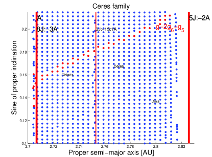
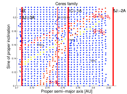
Figure 1: Dynamical maps for the orbital region of Ceres obtained by integrating test particles under the influence of all planets (panel A), and all planets and Ceres as a massive body (panel B). Unstable regions associated with mean-motion resonances appear as vertical strips. Secular resonance appear as inclined bands of aligned dots. Dynamically stable regions are shown as uniformly covered by blue dots. Vertical lines display the location of the main mean-motion resonances in the area. Red filled dots in both panels show the locations of “likely resonators” in the $g-2g_{6}+g_{5}$ secular resonance. Yellow and orange filled dots in panel B show the orbital locations of likely resonators in the linear secular resonances with Ceres of pericenter and node, respectively. The orbital location of 1 Ceres, 668 Dora, and 410 Chloris are labeled.

Ceres is the only dwarf planet in the asteroid belt. While its mass is not large enough to clear its orbital neighborhood, significant dynamical perturbations are expected from this body, either as a consequence of close encounters (Carruba et al., 2003) or because of linear secular resonances involving the precession frequency of Ceres node $s_{C}$ or pericenter $g_{C}$, and those of a given asteroid (Novaković et al., 2015). To investigate the importance of Ceres as a perturber, we obtain proper elements for 1400 particles in the plane of proper semi-major axis and inclination $(a,\sin{(i)})$, with the approach described in Carruba (2010), based on the method for obtaining synthetic proper elements of Knežević and Milani (2003). We integrated the particles over 20 Myr under the gravitation influence of i) all planets and ii) all planets plus Ceres as a massive body with $SWIFT\_MVSF$, the symplectic integrator based on $SWIFT\_MVS$ from the Swift package of Levison and Duncan (1994), and modified by Brož (1999) to include online filtering of osculating elements. The initial osculating elements of the particles went from 2.696 to 2.832 au in $a$ and from $5.5^{\circ}$ to $13.3^{\circ}$ in $i$. We used 35 intervals in $a$ and 40 in $i$. The other orbital elements of the test particles were set equal to those of Ceres at the modified Julian date of 57200.

Fig. 1 displays our results, as two dynamical maps. Each blue dot is associated with a particle proper $(a,\sin{(i)})$ value. For the case without Ceres as a massive body, displayed in panel A, the orbital region near Ceres is relatively stable. The only important non-linear secular resonance in the region is the $g-2g_{6}+g_{5}$ (or $2{\nu}_{6}-{\nu}_{5}$, in terms of linear secular resonances). Objects whose pericenter frequency is within $\pm 0.3$ arcsec/yr from $2g_{6}+g_{5}=52.229$ arcsec/yr, likely resonators in the terminology of Carruba (2009), are shown as red full dots in this figure. This is a diffusive secular resonance, and asteroids captured into this resonance may drift away, but will not be destabilize (Carruba et al., 2014). The situation is much different and more interesting for the map with Ceres as a massive body.

As observed in Fig. 1, panel B, accounting for Ceres causes the appearance of a 1:1 mean-motion resonance with this dwarf planet. Most importantly, linear secular resonances of nodes $s-s_{C}$ and pericenter $g-g_{C}$, first detected by Novaković et al. (2015) significantly destabilize the orbits in the proximity of Ceres. Combined with the long-term effect of close encounters with Ceres, this has interesting consequences for the survival of members of the Ceres family in the central main belt. Not many family members are expected to survive near Ceres, and this would cause significant difficulties in using standard dynamical family identification techniques, since they are based on looking for pairs of neighbors in proper element domains (Hierarchical Clustering Method, HCM hereafter, Bendjoya and Zappalá (2002)). Since the close neighbors of Ceres would have been removed on a short timescale, only objects whose distance from Ceres is higher than the average distance between pairs of asteroids in the central main belt would have survived. Also, the area at higher inclination than that associated with the linear secular resonances with Ceres should be significantly depleted of asteroids, and this is actually observed (see for instance Fig. 9 in Nesvorny et al. (2015)). Finally, the Dora family, a large ($\simeq 1260$ members, Nesvorny et al. (2015)) group of the same spectral type of Ceres, Ch, is located at lower inclinations than that of Ceres. Considering that the large Ch Chloris family is also encountered in the central main belt near Ceres, discriminating between a Ch asteroid from Ceres and one from Dora, Chloris, or other local sources would be a very daunting task, also considering that there are currently no identified members of a Ceres family that could serve as a basis for a taxonomical analysis.

To further investigate the efficiency of Ceres in perturbing its most immediate neighbors, we also performed numerical simulations of a fictitious Ceres family with the $SYSYCE$ integrator (Swift$+$Yarkovsky$+$Stochastic YORP$+$Close encounters) of Carruba et al. (2015a), modified to also account for past changes in the values of the solar luminosity. This integrators accounts for both the diurnal and seasonal version of the Yarkovsky effect, the stochastic version of the YORP effect, and close encounters of massless particles with massive bodies. The numerical set-up of our simulations was similar to what discussed in Carruba et al. (2015a): we used the optimal values of the Yarkovsky parameters discussed in Brož et al. (2013) for C-type asteroids, the initial spin obliquity was random, and normal reorientation timescales due to possible collisions as described in Brož (1999) were considered for all runs. We integrated our test particles under the influence of all planets (case A), and all planets plus Ceres (case B), and obtained synthetic proper elements with the approach described in Carruba (2010).

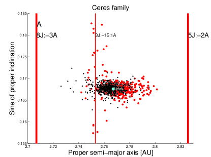
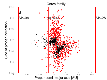
Figure 2: Projection in the proper $(a,\sin{(i)})$ plane of the initial (black full dots, $T=1.2$ My) and final (red full dots, $T=455.6$ My) elements of the simulated Ceres family members integrated under the gravitational influence of all planets (panel A), and all planets plus Ceres (panel B). Vertical lines display the location of the mean-motion resonances, the cyan full dot identify the orbital location of Ceres itself.

The fictitious Ceres family was generated with the approach described in Vokrouhlický et al. (2006): we assumed that the initial ejection velocity field follows an isotropical Gaussian distribution of zero mean and standard deviation given by:

$${\sigma}_{V_{ej}}=V_{EJ}\cdot\frac{5km}{D},$$ (1)

where $D$ is the body diameter in km, and $V_{EJ}$ is a parameter describing the width of the velocity field. We used the relatively small value of $V_{EJ}=60$ m/s for our simulated family. In the next section we will discuss why it is quite likely that any possible Ceres family would have a much larger value of $V_{EJ}$. Since here, however, we were interested in the dynamics in the proximity of Ceres itself, our choice of $V_{EJ}$ was, in our opinion, justified. We generated 642 particles with size-frequency distributions (SFD) with an exponent $-\alpha$ that best-fitted the cumulative distribution equal to 3.6, a fairly typical value (Masiero et al., 2012), and with diameters in the range from 2.0 to 12.0 km.

Fig. 2 displays our results in the proper $(a,\sin{(i)})$ plane for the simulation without Ceres as a massive body (panel A) and with a massive Ceres (panel B). Black full dots display the position of simulated Ceres family members at the beginning of the simulation, after 1.2 My, while the red full dots show the orbital location at the end of the integration, for $T=455.6$ My. For the case without Ceres one can notice that the family does not disperse much, and that most of the scattering is caused by the 3J:-1S:1A three-body resonance. Results including Ceres as a perturber are quite more interesting: already after just 1.2 My secular resonances with Ceres cleared a gap near the orbital location of the dwarf planet, identified by a full blue dot. The situation is even more dramatic at the end of the simulation, where we observe that Ceres scattered material at lower and higher inclinations with respect to the case in which Ceres had no mass, and opened a significant gap at the family center, as also observed in the dynamical map of Fig. 1, panel B.

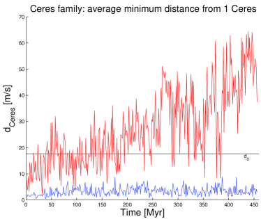
Figure 3: Averaged minimum distance from Ceres $d_{Ceres}$ as a function of time of the simulated family members for the case without (blue line) and with (red line) Ceres as a massive body. The horizontal black line displays the maximum nominal distance cutoff level $d_{0}$ for the whole simulated Ceres family.

How difficult would be to identify our simulated Ceres family using HCM? To answer this question, we computed the nominal distance velocity cutoff $d_{0}$ for which two nearby asteroids are considered to be related using the approach of Beaugé and Roig (2001), that defines this quantity as the average minimum distance between all possible asteroid pairs, as a function of time, for i) all paired asteroids in the simulated Ceres family ($d_{0}$), and ii) just with respect to Ceres itself ($d_{Ceres}$). This latter quantity provides an estimate of the minimum value of distance cutoff needed to identify a Ceres family using the standard HCM. The maximum value of the nominal distance velocity cutoff for the simulated Ceres family was equal to 17.7 m/s. When Ceres was not considered as a massive body, values of $d_{Ceres}$ were of the order of 5 m/s, at all times below the nominal distance velocity cutoff (see Fig. 3, blue line). Once Ceres was included as a massive body, however, values of $d_{Ceres}$ quickly surpassed the nominal distance velocity cutoff $d_{0}$ (see red line in Fig. 3): after 200 My, except of short episodes in which $d_{Ceres}<d_{0}$, for most of the time $d_{Ceres}$ was larger than $d_{0}$. After 380 My, this trend was consolidated and $d_{Ceres}$ was always larger than $d_{0}$. The identification of a Ceres family using HCM in the domain of proper elements of the simulated family and Ceres as the first body would be quite challenging after 380 My.

So, where to look for hypothetical surviving members of a Ceres family? The next section will be dealing with estimating the extent of the initial orbital dispersion of a putative family, and in assessing the regions where locating its members could be easier.

3 Ejection velocities of a possible Ceres family

The escape velocity $V_{esc}$ from Ceres is considerably larger than that of other, less massive bodies: $\simeq 480$ m/s (Russell et al., 2015) versus the 360 m/s for Vesta (Russell et al., 2012), the largest body in the main belt with a uncontroversial recognized asteroid family. The Vesta family is one of the largest in the main belt, and one would expect a putative Ceres family to be even larger.

Recently, Carruba and Nesvorný (2016) investigated the shape of the ejection velocity field of 49 asteroid families. Typical observed values of $\beta=V_{EJ}/V_{esc}$, with $V_{EJ}$ given by Eq. 1, are between 0.5 and 1.5 (see also Nesvorny et al. (2015), sect. 5). While for typical asteroid families this implies that $V_{EJ}$ is generally lower than 100 m/s, even a conservative choice of $\beta=0.5$ for Ceres would produce a field with $V_{EJ}$ of the order of 240 m/s. This is more than a factor of 2 larger than the higher values of $V_{EJ}$ observed for some of the oldest asteroid families (Carruba et al., 2015b), but not inconsistent with the observed presence of crater ray systems around large craters on Ceres, such as Occator (Nathues et al., 2015), that cover a large portion of the Ceres surface. Since the circular velocity needed to form such rays is of the order of half the escape velocity from Ceres, this suggests that values of $\beta$ near 0.5 for the $V_{EJ}$ parameter of a possible Ceres family are not unreasonable. Following the approach of Vokrouhlický et al. (2006), see also Carruba et al. (2015b), we generated fictitious Ceres asteroids members with diameters 1, 3, and 7 km with the minimum and maximum value of $\beta$ from Carruba and Nesvorný (2016).

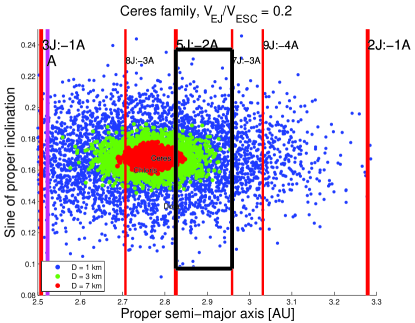
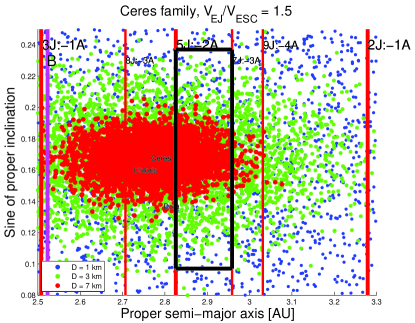
Figure 4: An $(a,sin(i))$ distribution of $D=1,3,$ and $7$ km members of Ceres families obtained using $V_{EJ}=0.2V_{ESC}$ (panel A) and $V_{EJ}=1.5V_{ESC}$ (panel B). The black box identify the orbital regions in which most of the $D=3$ km fragments for $V_{EJ}=1.5\cdot V_{ESC}$ and most of the $D=1$ km for $V_{EJ}=0.2\cdot V_{ESC}$ could be found in the pristine region of the main belt.

Fig. 4 displays our results for $\beta=0.2$ (panel A) and $\beta=1.5$ (panel B). Even in the most conservative case of $\beta=0.2$, a value lower than those of any of the families studied in Carruba and Nesvorný (2016), we still found that a significative fraction of the multi-km (and potentially observable) fragments from Ceres could have been injected in the pristine region of the main belt. We define this region as the area between the 5J:-2A and 7J:-3A mean-motion resonances with Jupiter. Because of these two dynamical barriers, very little material from external regions can reach this area (Brož et al., 2013). As a consequence, the local density of asteroids is much inferior to that of other regions of the asteroid belt. Also, only small C-type families, such those of Naema (301 members), Terpsichore (138 members), and Terentia (79 members) (Nesvorny et al., 2015) are found in the region, and at eccentricity values quite different than that of Ceres, so easily distinguishable from putative Ceres fragments. If any large ($D>5$ km), not easily movable by non-gravitation effects, members of a hypothetical Ceres family would have been injected in this region after the LHB, it would be reasonable to expect that they could have remained there and still be visible today. We selected a region in the pristine zone where most of the $D>1$ km objects could be found, according to our results for the most conservative case with $\beta=0.2$ (black box in Fig. 4, panels A, this also corresponds to the region in which most of the $D>3$ km objects would be located in the most optimistic scenario of $\beta=1.5$, see black box in Fig. 4, panels B. In the next section we will investigate if any such object could be identified in the pristine region.

4 The pristine region

Results of a dynamical map with Ceres as a massive body, not shown for the sake of brevity, demonstrate that the pristine region at inclination close to that of Ceres is dynamically stable, with no linear secular resonances with Ceres and only minor diffusive secular resonances with the giant planets. In the black region of Fig. 4 there are four Ch asteroids, according to data from the three major photometric/spectroscopic surveys (ECAS (Eight-Color Asteroid Analysis, Tholen et al. (1989)), SMASS (Small Main Belt Spectroscopic Survey, Bus and Binzel (2002a, b)), and S3OS2 (Small Solar System Objects Spectroscopic Survey, Lazzaro et al. (2004)): 195 Eurykleia, 238 Hypatia, 910 Annelise, and 1189 Terentia. The WISE survey (Masiero et al., 2012) estimates that these objects have diameters of 85.7, 148.5. 47.1, and 55.9 km, respectively. With the possible and very doubtful exception of Annelise and Terentia, the other objects are too big to be realistically assumed to be members of a Ceres family. Apart from a small family of 79 members around Terentia (Nesvorny et al., 2015), no major family has been identified around the largest objects, that appear to be isolated. To increase statistics, we turn our attention to photometric data from the Sloan Digital Sky Survey-Moving Object Catalog data, fourth release (SDSS-MOC4 hereafter, Ivezić et al. (2001)). Using the classification method of DeMeo and Carry (2013) in the $gri$ slope and $z^{\prime}-i^{\prime}$ colors domain, we identified 23 C-type photometric candidates in the pristine region.

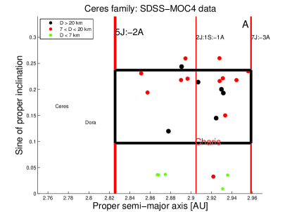
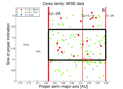
Figure 5: An $(a,\sin{(i)})$ projection of 23 C-type SDSS-MOC4 photometric candidates (panel A) and 130 objects with WISE albedo in the range from 0.08 to 0.10 (panel B) in the pristine region. Candidates of different diameters are shown with the color code reported in the figure legend. The orbital location of 627 Charis is identified by its name, in red letters.

Fig. 5, panel A shows their orbital location in the $(a,\sin{(i)})$ plane. Vertical red lines display the orbital location of the main mean-motion resonances in the region, including the 2J:1S:-1A three-body resonance that divides the pristine area in two parts. 14 of the 23 SDSS C-type asteroids, 60.9% of the total, can be found in the black region where we would expect Ceres family members to be located. By contrast, only 6 objects can be found at lower inclinations, and only 3 at higher values. Overall, C-type photometric candidates in the pristine region tend to cluster at inclination values close to that of Ceres.

To check the statistical significance of this result, we checked what would be the probability that these 14 asteroids were produced by a fluctuation of a Poisson distribution (it has been suggested that the orbital distribution of background asteroids follows a Poisson distribution Carruba and Machuca (2011)). Following the approach of Carruba and Machuca (2011), the probability that the expected number of $k=14$ occurrences in a given interval is produced by the Poissonian statistics is given by

$$f(k,\lambda)=\frac{{\lambda}^{k}e^{-\lambda}}{k!},$$ (2)

where $\lambda$ is a positive real number, equal to the expected number of occurrences in the given interval. Here we used for $\lambda$ the number of SDSS candidates in the black region ($N_{SDSS}=14$), weighted to account for the volume occupied by the region ($V_{Reg}$) with respect to the total volume considered in our analysis ($V_{Tot}$, we considered asteroids with $\sin{(i)}<0.35$). This is given by:

$$\lambda=N_{SDSS}\frac{V_{Reg}}{V_{Tot}},$$ (3)

For our considered black region, this yield $\lambda=5.6$, that corresponds to a probability to observe 14 bodies of just 0.13%, quite less than the null hypothesis level of 1.0% of the data being drawn from the Poisson distribution. Similar analysis performed for uniform and Gaussian distributions (see Carruba and Machuca (2011) for details on the procedures) also failed to fulfill the null hypothesis, which suggests that the observed concentration of asteroids at inclinations close to those of Ceres should be statistically significant.

To increase the number of possible Ceres members, we also look for objects in the WISE database whose geometric albedo $p_{V}$ is between 0.08 and 0.10, the range of albedo values observed for more than 90% of the surface material at Ceres by the Dawn spacecraft (Li et al., 2015). While C-type objects with these values of WISE albedo could be associated with a Ceres family, other spectral types such as X, D, L, K, and even some S also have albedo values in this range, so this data must be considered with some caution. Nevertheless, it provides useful preliminary information. After eliminating objects belonging to spectral types other than C (13 bodies), members of the Terpsichore and Terentia families (7 asteroids), and of the X-type group Charis (5 objects), we were left with a sample of 130 asteroids in that range of albedos. The fact that only 4 C-type candidates were members of the Terpsichore family, and 3 of Terentia, 3.2% of the total, seems to indicate that local sources may not explain all the local population of C-type candidates. Since the other C-type objects in the region have diameters less than that of Terpsichore, even if they produced families in the past (of which there is no trace today), we would expect that to account at most for 10% of the observed population of C-type candidates.

Fig. 5, panel B, displays the $(a,\sin{(i)})$ distribution of these objects. Again, 67 asteroids, 51.5% of the total, are found in the black region, while 39, (30.0%) are found at lower inclinations and 24 (18.5%) at higher $i$. 22 of the objects at low inclinations cluster near the X-type family Charis, and could quite possibly be associated with its halo. If we eliminate these objects, then the percentage of albedo candidates in the black region increase to 56.0%, a result similar to that from the SDSS-MOC4 data. To reduce possible contaminations from the local large families of Charis, Eos and Koronis, which could have small populations of objects with WISE albedos in the studied range, we eliminated objects i) with $a$ beyond the 2J:1S:-1A mean-motion resonance that could potentially be associated with the Charis and Eos halo (Brož and Morbidelli, 2013), and are less likely to have been produced by collisions on Ceres with low values of $\beta$, and ii) those objects between the 5J:-2A and the 2J:1S:-1A mean-motion resonances with proper eccentricities lower than 0.08 and sine of proper inclinations lower than 0.06, that could potentially be members of the Koronis halo (Carruba et al., 2016b).

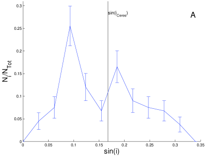
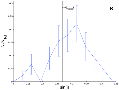
Figure 6: A histogram of the distribution of $\sin{(i)}$ values for 133 and 45 C-type (panel A and B, respectively) albedo candidates in the pristine region. The vertical line marks the value of Ceres inclination. Errors are assumed to be proportional to the square root of the number of asteroids in each size bin.

Fig. 6 shows a histogram of all the 133 C-type albedo candidates in the pristine region (panel A), and of the 45 asteroids that satisfied our criteria (panel B). In the first panel one can notice a peak at $\sin(i)\simeq 0.10$ associated with the local Charis X-type family, that is not visible once objects in the Charis halo are removed (panel B). Remarkably, there is a peak in the $\sin{(i)}$ distribution that nearly coincides with the current value of the inclination of Ceres. To check for its statistical significance, and in particular if it could be the product of fluctuations in a Poisson probability distribution, we used the approach described in Carruba and Machuca (2011), Sect. 4.1. For the $N_{i}$ values of the number of asteroids per size bin in the histogram shown in Fig. 6, panel B, we best-fitted the value of $\lambda$ in Eq. 2 using the $MATLAB$ routine (where $MATLAB$ stands for Matrix Laboratory) poissfit. We then generated 1000 random populations of asteroids following the Poisson distribution with the routine poissrnd, and then performed a Pearson ${\chi}^{2}$ test by computing the ${\chi}^{2}$-like variable defined as:

$${\chi}^{2}=\sum_{i=1}^{n_{int}}\frac{(q_{i}-p_{i})^{2}}{q_{i}},$$ (4)

where $n_{int}$ is the number of intervals used in the histogram in Fig. 6, panel B with a number of objects larger than 0 (9), $q_{i}$ is the number of real objects in the $i-th$ interval, and $p_{i}$ is the number of simulated asteroids in the same $\sin{(i)}$ range. Assuming that the ${\chi}^{2}$-like variable follows an incomplete gamma function probability distribution, the probability of the two distributions being compatible can be computed considering the minimum value of ${\chi}^{2}$ (17.46, in our case) and the number of degrees of freedom (9, Press (2001)). This yields a probability of 0.8% of the two distributions being compatible, below the null hypothesis, which implies that the observed peak should be statistically significant. Similar results were obtained for the uniform and Gaussian distributions.

While not a conclusive proof of the possible existence of a Ceres family, this interesting result represents, in our opinion, a circumstantial evidence in favor of this possibility. A list of the photometric and albedo Ceres members candidates with diameters less than 20 km in the pristine region identified in this work is provided in Table LABEL:table:_Ceres_members.

5 Conclusions

Our results could be summarized as follows:

• We studied the effect that the local dynamics may have had on a possible Ceres family in the central main belt. Resonances with Ceres would have depleted the population of members at higher inclinations than Ceres itself, and close encounters with the dwarf planet would also caused further spread of the family, making the identification of a Ceres dynamical group impossible after timescales of 200-400 My. Members of the Ceres family at low inclinations would not be easily distinguishable from members of other local large Ch families such as Dora and Chloris.

• We investigated the original spread that a Ceres family may have had in the $(a,e,\sin{(i)})$ proper element domain. Assuming that values of the initial ejection velocity parameter $\beta=V_{EJ}/V_{esc}$, would be in the range observed for other families, we expect that a potentially observable population of $D>3$ km fragments, likely the results of the formation of craters on Ceres larger than 300-400 km, should have been injected into the pristine region of the main belt. Collisional models predict that about 10 such craters could have formed on Ceres (Marchi et al., 2016). While the largest well-defined basins observed by Dawn on Ceres surface are smaller than 300 km, there is topographical evidence that larger impact structures formed in the ancient past (Marchi et al., 2016). The pristine region is characterized by a lower number density of asteroids, when compared to the central main belt. We argue that Ceres family members would be easier to recognize in this region, rather than near Ceres itself.

• We analyzed which objects in the pristine region have taxonomical, photometric, or albedo data comparable to that of Ceres. Remarkably, C-type candidates in this region cluster at inclinations that would be compatible with the range reached by possible Ceres’ fragments. Among albedo C-type candidates, we observe a statistically significant peak in the $\sin{(i)}$ distribution at values close to that of Ceres itself. The number of C-type candidates at lower and higher inclinations is significantly lower, and no significant local sources can produce the observed distribution of C-type candidates.

While we believe that we have provided a circumstantial evidence in favor of a possible Ceres family in this work, we are aware that we have not proven its existence beyond any reasonable doubt. Since Ceres surface is characterized by a distinct $3\mu m$ absorption band (de Sanctis et al., 2015), observing this feature in some of the proposed Ceres family candidates could be a conclusive proof that such family exist, or existed in the past. Should the existence of a Ceres family be finally proved, future lines of research could investigate the possibility of some main belt comets (Hsieh, 2015) being escaped members of this long-lost asteroid group.

Table 1: Photometric and albedo Ceres family candidates in the pristine region with $D<20$ km. We report the asteroid identification, its proper $a,e,\sin{(i)}$, its absolute magnitude $H$, the estimated diameter $D$, and if it is a photometric (SDSS) or an albedo (WISE) C-type candidate. Asteroids in the expected inclination range of the Ceres family are marked with a dagger $(\dagger)$. The 45 asteroids that satisfied our selection criteria for Fig. 6, panel B, have their identifications marked in bold.

Identification	Semi-major axis [au]	Eccentricity	Sine of inclination	Absolute magnitude	Diameter [km]	Type
2082	2.921907	0.193664	0.032701	13.30	17.12	SDSS
5994 $(\dagger)$	2.851295	0.184111	0.230810	11.98	17.80	SDSS
6671	2.894602	0.135151	0.259412	12.54	13.75	SDSS
6721	2.928060	0.160947	0.290183	12.40	14.93	WISE
8560 $(\dagger)$	2.956013	0.055937	0.234792	12.30	18.95	SDSS
8706 $(\dagger)$	2.847802	0.081223	0.142328	13.30	9.59	WISE
11771 $(\dagger)$	2.916868	0.182122	0.123918	13.90	7.60	WISE
12356	2.935904	0.069843	0.035674	13.10	6.01	SDSS
12986 $(\dagger)$	2.930536	0.071421	0.192957	13.90	7.77	WISE
14037 $(\dagger)$	2.846048	0.113655	0.173687	12.80	12.86	WISE
14338 $(\dagger)$	2.944557	0.079173	0.217839	12.40	8.99	SDSS
14531 $(\dagger)$	2.833541	0.136888	0.098603	13.80	8.12	WISE
16885 $(\dagger)$	2.890294	0.089698	0.218012	12.90	15.54	SDSS
18198 $(\dagger)$	2.928039	0.165372	0.216076	13.60	9.67	SDSS
18463	2.856107	0.121585	0.027381	14.40	5.89	WISE
20094 $(\dagger)$	2.861264	0.126932	0.185285	14.40	6.16	WISE
20095	2.867089	0.044780	0.036435	14.44	5.73	SDSS
20965 $(\dagger)$	2.929609	0.106764	0.250502	13.20	10.62	WISE
21714 $(\dagger)$	2.896649	0.056614	0.220559	12.50	8.27	SDSS
22540	2.874836	0.064495	0.036984	14.00	3.60	SDSS
23000 $(\dagger)$	2.931225	0.042298	0.221314	13.90	14.06	SDSS
23136	2.927916	0.115123	0.259867	13.50	8.05	SDSS
23432	2.910407	0.099806	0.060429	15.00	4.32	WISE
26085	2.847349	0.071938	0.052672	14.20	6.12	WISE
28297 $(\dagger)$	2.933505	0.149849	0.150057	13.60	9.36	SDSS
29514	2.936161	0.193732	0.290663	13.20	10.40	WISE
29906 $(\dagger)$	2.884096	0.043687	0.210437	14.00	6.84	WISE
31232 $(\dagger)$	2.857460	0.055909	0.194055	14.40	7.27	SDSS
32421 $(\dagger)$	2.915570	0.131466	0.183926	13.70	8.45	WISE
32586 $(\dagger)$	2.905601	0.142687	0.168171	12.80	11.24	WISE
33202	2.931046	0.058748	0.009448	14.46	5.68	SDSS
34129	2.868182	0.042556	0.036113	15.00	4.11	SDSS
35533 $(\dagger)$	2.902357	0.098794	0.100204	14.50	5.91	WISE
38466	2.860576	0.046388	0.037292	15.10	4.09	WISE
42544	2.914965	0.087749	0.092480	14.70	4.85	WISE
42710 $(\dagger)$	2.939916	0.070241	0.191939	13.90	7.49	WISE
43235 $(\dagger)$	2.835135	0.069649	0.229597	14.00	6.72	WISE
44357	2.938663	0.176620	0.068078	14.50	5.65	WISE
46645	2.944500	0.159099	0.091087	14.00	6.97	WISE
47651 $(\dagger)$	2.836642	0.070337	0.213856	14.60	5.36	WISE
47862 $(\dagger)$	2.887313	0.087727	0.202313	14.30	6.29	WISE
51050 $(\dagger)$	2.876180	0.169556	0.197835	14.00	6.87	WISE
51338 $(\dagger)$	2.947534	0.178943	0.161967	13.10	11.14	WISE
51707 $(\dagger)$	2.893943	0.194367	0.117033	14.50	5.82	WISE
53875 $(\dagger)$	2.895506	0.046369	0.211182	13.70	8.32	WISE
54065 $(\dagger)$	2.948372	0.120630	0.187491	15.00	4.25	WISE
54930 $(\dagger)$	2.915907	0.102511	0.199583	14.90	4.42	WISE
54966 $(\dagger)$	2.928465	0.101667	0.098231	14.50	5.30	WISE
55903	2.941553	0.124014	0.300482	14.50	5.68	WISE
57676	2.840613	0.081003	0.094847	15.40	3.51	WISE
57695	2.953239	0.067685	0.026310	15.20	4.28	WISE
61674 $(\dagger)$	2.856602	0.145630	0.134328	13.70	8.21	WISE
65774	2.876079	0.084274	0.023299	15.40	3.89	WISE
66046	2.923553	0.054957	0.284802	13.80	7.83	WISE
66648 $(\dagger)$	2.857988	0.126132	0.189854	15.50	3.57	WISE
67333 $(\dagger)$	2.884682	0.186828	0.115222	14.00	7.41	WISE
71263 $(\dagger)$	2.851656	0.166470	0.153571	13.90	7.29	WISE
72691 $(\dagger)$	2.954464	0.092571	0.199377	14.40	5.88	WISE
74398	2.926309	0.113313	0.313344	13.20	9.78	WISE
76814	2.854806	0.079048	0.288523	13.90	7.56	WISE
77346	2.925627	0.114702	0.090742	15.30	3.93	WISE
77873 $(\dagger)$	2.943052	0.183550	0.103473	14.10	6.63	WISE
82715 $(\dagger)$	2.831806	0.085409	0.194841	13.90	6.99	WISE
82897 $(\dagger)$	2.878531	0.056788	0.210677	14.50	5.69	WISE
83337 $(\dagger)$	2.831666	0.098578	0.099738	14.30	6.24	WISE
83707	2.830936	0.085110	0.092492	14.00	6.80	WISE
85114	2.835897	0.132118	0.277561	15.10	4.20	WISE
88573 $(\dagger)$	2.919644	0.132783	0.162074	14.40	5.92	WISE
88723	2.834080	0.088113	0.088653	14.90	4.69	WISE
89727	2.945443	0.101456	0.017127	15.40	3.75	WISE
91870 $(\dagger)$	2.845707	0.116806	0.164315	14.70	5.11	WISE
91997 $(\dagger)$	2.921480	0.078832	0.113695	14.80	5.09	WISE
97020	2.901140	0.058409	0.274274	14.10	7.04	WISE
103529	2.920771	0.052655	0.088095	15.50	3.36	WISE
103923 $(\dagger)$	2.933675	0.076817	0.172426	15.40	3.61	WISE
104028 $(\dagger)$	2.923278	0.054426	0.189286	14.60	5.39	WISE
105129 $(\dagger)$	2.862443	0.199475	0.134897	15.00	4.70	WISE
108386 $(\dagger)$	2.956425	0.080106	0.173829	15.20	4.10	WISE
111331	2.917046	0.091109	0.083911	15.20	4.21	WISE
111394 $(\dagger)$	2.946302	0.090717	0.124884	14.50	5.73	WISE
112976 $(\dagger)$	2.878561	0.086200	0.121019	14.90	4.56	WISE
113564	2.851523	0.085304	0.087892	14.80	4.78	WISE
119722	2.852195	0.072637	0.046523	15.30	3.92	WISE
120043 $(\dagger)$	2.927114	0.071038	0.193386	14.60	5.40	WISE
121281	2.844024	0.150695	0.095594	15.00	4.65	WISE
125857	2.896361	0.102890	0.090084	15.70	3.28	WISE
128714	2.868729	0.041501	0.290199	14.40	5.81	WISE
129048 $(\dagger)$	2.848874	0.132366	0.220818	14.90	4.71	WISE
130023 $(\dagger)$	2.880666	0.139291	0.156271	14.80	5.14	WISE
131267 $(\dagger)$	2.848184	0.130562	0.184916	14.90	4.57	WISE
133841	2.932969	0.065715	0.086641	14.90	4.47	WISE
139184 $(\dagger)$	2.915685	0.191200	0.137376	15.60	3.20	WISE
139793	2.953216	0.076844	0.095644	15.30	3.72	WISE
140007	2.841540	0.052047	0.048892	14.60	5.45	WISE
140769 $(\dagger)$	2.860013	0.068603	0.209332	15.20	4.21	WISE
143166	2.869961	0.101913	0.049494	15.30	3.81	WISE
144712 $(\dagger)$	2.915620	0.171867	0.019665	15.90	2.85	WISE
144715 $(\dagger)$	2.872016	0.110133	0.171309	15.40	3.73	WISE
145325 $(\dagger)$	2.849511	0.122737	0.125786	15.20	4.14	WISE
145392	2.902675	0.059978	0.305121	14.80	5.07	WISE
155547	2.935295	0.076924	0.086005	15.30	3.88	WISE
159263	2.851540	0.121195	0.256403	15.40	3.66	WISE
166760	2.945129	0.099172	0.082949	15.00	4.22	WISE
169161	2.889445	0.116778	0.062533	15.90	3.04	WISE
172377 $(\dagger)$	2.902666	0.179680	0.154193	14.80	4.62	WISE
174489	2.929807	0.132278	0.293032	14.90	4.48	WISE
176347 $(\dagger)$	2.918230	0.086535	0.126204	14.80	4.77	WISE
178669	2.956492	0.110930	0.083905	15.50	3.57	WISE
181605 $(\dagger)$	2.87433	0 0.158614	0.102414	15.30	4.01	WISE
182687	2.910644	0.119178	0.095378	15.50	3.38	WISE
184356	2.908767	0.107959	0.091759	15.50	3.43	WISE
184487	2.945952	0.095575	0.087735	16.10	2.61	WISE
189495	2.944911	0.133490	0.293474	14.30	6.32	WISE
191486	2.947722	0.145902	0.256494	14.60	5.36	WISE
192044	2.940902	0.074702	0.252544	14.70	5.04	WISE
197144	2.925675	0.105006	0.088102	15.00	4.34	WISE
198403 $(\dagger)$	2.906537	0.088144	0.185480	15.50	3.37	WISE
198808 $(\dagger)$	2.924283	0.073838	0.238708	14.60	5.27	WISE
201824	2.876024	0.082627	0.248968	14.90	4.54	WISE
214826	2.949845	0.113408	0.084030	15.80	3.03	WISE
218273	2.887695	0.078069	0.087647	15.50	3.70	WISE
218776 $(\dagger)$	2.924260	0.057623	0.134816	15.60	3.38	WISE
222080 $(\dagger)$	2.866610	0.149922	0.190036	16.10	2.68	WISE
227004 $(\dagger)$	2.913158	0.058757	0.135286	15.20	3.93	WISE
231791 $(\dagger)$	2.889728	0.157418	0.214961	14.90	4.84	WISE
232724	2.903389	0.120023	0.091075	15.50	3.66	WISE
235975	2.920486	0.101497	0.095416	15.30	3.77	WISE
236004 $(\dagger)$	2.943159	0.076640	0.183347	15.30	3.67	WISE
238734 $(\dagger)$	2.957799	0.056591	0.189721	15.60	3.26	WISE
239518	2.859584	0.120313	0.258105	15.40	3.50	WISE
239993 $(\dagger)$	2.955953	0.053980	0.206900	15.20	3.98	WISE
240384	2.834916	0.123127	0.261325	16.30	2.45	WISE
243283	2.890796	0.122268	0.073358	16.40	2.45	WISE
243302 $(\dagger)$	2.938414	0.125304	0.208466	15.90	3.06	WISE
243774	2.906543	0.130365	0.295275	14.90	4.43	WISE
243854 $(\dagger)$	2.947074	0.198642	0.126632	15.70	3.30	WISE
244955 $(\dagger)$	2.899970	0.057671	0.168345	15.50	3.50	WISE
245480	2.858417	0.093258	0.262532	15.60	3.50	WISE
246409	2.929076	0.145512	0.055515	15.90	2.84	WISE
246466	2.830511	0.084131	0.085150	16.10	2.64	WISE
246720	2.911652	0.076910	0.092850	16.10	2.82	WISE
247195	2.847924	0.120740	0.261754	15.90	2.98	WISE
248035 $(\dagger)$	2.929195	0.139209	0.122659	15.80	3.00	WISE
248581	2.920784	0.100786	0.076717	15.70	3.20	WISE
249201	2.916190	0.077005	0.087743	15.70	3.08	WISE
249283 $(\dagger)$	2.894856	0.105884	0.214428	16.10	2.72	WISE
250010 $(\dagger)$	2.896574	0.126868	0.098989	16.20	2.58	WISE
260891 $(\dagger)$	2.945898	0.111076	0.172986	15.80	3.22	WISE
261489	2.883625	0.146659	0.302045	15.60	3.21	WISE
268622 $(\dagger)$	2.858875	0.075933	0.127763	16.20	2.58	WISE

References

- Beaugé and Roig (2001) Beaugé, C., Roig, F., 2001, Icarus, 153, 391.
- Bendjoya and Zappalá (2002) Bendjoya, P., Zappalà, V. 2002. Asteroids III, Univ. of Arizona Press, Tucson, 613.
- Brasil et al. (2015) Brasil, P. I. O., Roig, F., Nesvorný, D., Carruba, V., Aljbaae, S., Huaman, M. E., 2015, Icarus, 266, 142.
- Brož (1999) Brož, M., 1999. Thesis, Charles Univ., Prague, Czech Republic.
- Brož and Morbidelli (2013) Brož, M., Morbidelli, A. 2013. Icarus, 223, 844.
- Brož et al. (2013) Brož, M., Morbidelli, A., Bottke, W. F., Rozenhal, J., Vokrouhlický, D, Nesvorný, D. 2013. A&A, 551, A117.
- Bus and Binzel (2002a) Bus, J. S., Binzel, R. P. 2002a. Icarus 158, 106.
- Bus and Binzel (2002b) Bus, J. S., Binzel, R. P. 2002b. Icarus 158, 146.
- Carruba et al. (2003) Carruba, V., Burns, J. A., Bottke, W., Nesvorný, D. 2003. Icarus, 162, 308.
- Carruba (2009) Carruba 2009. MNRAS, 395, 358.
- Carruba (2010) Carruba, V. 2010. MNRAS, 408, 580.
- Carruba and Machuca (2011) Carruba, V., Machuca, J. F., MNRAS, 418, 1102.
- Carruba et al. (2014) Carruba, V., Huaman, M. E., Domingos, R. C., Santos, C. R. D., & Souami, D. 2014, MNRAS, 439, 3168.
- Carruba et al. (2015a) Carruba, V., Nesvorný, D., Aljbaae, S., Huaman, M. E., 2015a. MNRAS, 451, 4763.
- Carruba et al. (2015b) Carruba, V., Nesvorný, D., Aljbaae, S., Domingos, R. C., Huaman, M. E., 2015b. MNRAS, submitted.
- Carruba and Nesvorný (2016) Carruba, V., Nesvorný, D., 2016. MNRAS, 457, 1332.
- Carruba et al. (2016b) Carruba, V., Nesvorný, D., Aljbaae, S., 2016, Icarus, in press.
- DeMeo and Carry (2013) DeMeo, F., Carry, B., 2013. Icarus, 226, 723.
- de Sanctis et al. (2015) de Sanctis, M. C., Ammannito, E., Raponi, A., et al. 2015, Nature, 528, 241
- Fu et al. (2015) Fu, R., Ermakov, A., Zuber, M., Hager, B. 2015, AGU Fall Meeting, P23D-02.
- Hsieh (2015) Hsieh, H. H. 2015, arXiv:1511.01912.
- Ivezić et al. (2001) Ivezić, Ž., and 32 colleagues 2001. AJ, 122, 2749.
- Knežević and Milani (2003) Knežević, Z., Milani, A., 2003. A&A, 403, 1165.
- Lazzaro et al. (2004) Lazzaro, D., Angeli, C. A., Carvano, J. M., Mothé-Diniz, T., Duffard, R., Florczak, M. 2004. Icarus 172, 179.
- Levison and Duncan (1994) Levison, H. F., Duncan, M. J., 1994. Icarus, 108, 18-36.
- Li et al. (2015) Li, J.-Y., Le Corre, L., Reddy, V., et al. 2015, AAS/Division for Planetary Sciences Meeting Abstracts, 47, #103.04
- Marchi et al. (2001) Marchi, S., Dell’Oro, A., Paolicchi, P., Barbieri, C., 2001, A&A 374, 1135.
- Marchi et al. (2013) Marchi, S., Bottke, W. F., Cohen, B. A., et al. 2013, Nature Geoscience, 6, 303
- Marchi et al. (2016) Marchi, S. and 9 co-authors, 2016, Lunar Planet. Sci., submitted.
- Milani et al. (2014) Milani, A., Cellino, A., Kneževicć, Z., Novaković, B., Spoto, F., Paolicchi, P., 2014, Icarus, 239, 46.
- Masiero et al. (2012) Masiero, J. R., Mainzer, A. K., Grav, T., Bauer, J. M., Jedicke, R. 2012. ApJ, 759, 14.
- Nathues et al. (2015) Nathues, A., Hoffmann, M., Schaefer, M., et al. 2015, Nature, 528, 237
- Novaković et al. (2015) Novaković, B., Maurel, C., Tsirvoulis, G., Knežević, Z. 2015. ApJ, 807, L5.
- Nesvorny et al. (2015) Nesvorny, D., Broz, M., Carruba, V. 2015. In Asteroid IV, (P. Michel, F. E.De Meo, W. Bottke Eds.), Univ. Arizona Press and LPI, 297.
- Novaković et al. (2012) Novaković, B., Dell’Oro, A., Cellino, A., & Knežević, Z. 2012, MNRAS, 425,
- Press (2001) Press, V.H., Teukolsky, S. A., Vetterlink, W. T., Flannery, B. P., 2001, Numerical Recipes in Fortran 77, Cambridge Univ. Press, Cambridge. 338.
- Rivkin et al. (2014) Rivkin, A. S., Asphaug, E., Bottke, W. F., 2014. Icarus, 243, 429.
- Russell et al. (2012) Russell, C. T., McSween, H. Y., Jaumann, R., et al. 2012, AGU Fall Meeting Abstracts.
- Russell et al. (2015) Russell, C. T., Raymond, C. A., Nathues, A., et al. 2015, IAU General Assembly, 22, #2221738
- Tholen et al. (1989) Tholen, D. J., 1989. In Asteroid III, Binzel R. P., Gehrels, T., Matthews, M. S. (eds), University of Arizona Press, Tucson, 298.
- Vokrouhlický et al. (2006) Vokrouhlický, D., Brož, M., Morbidelli, A., Bottke, W. F., Nesvorný, D., Lazzaro, D., Rivkin, A. S. 2006. Icarus 182, 92.