Non-Boltzmann Ensembles and Monte Carlo Simulations

Abstract

Boltzmann sampling based on Metropolis algorithm has been extensively used for simulating a canonical ensemble and estimating macroscopic properties of a closed system at the desired temperature. An estimate of a mechanical property, like energy, of an equilibrium system, is made by averaging over a large number microstates generated by Boltzmann Monte Carlo methods. This is possible because we can assign a numerical value for energy to each microstate. However, a thermal property like entropy, is not easily accessible to these methods. The reason is simple. We can not assign a numerical value for entropy, to a microstate. Entropy is not a property associated with any single microstate. It is a collective property of all the microstates. Toward calculating entropy and other thermal properties, a non-Boltzmann Monte Carlo technique called Umbrella sampling was proposed some forty years ago. Umbrella sampling has since undergone several metamorphoses and we have now, multi-canonical Monte Carlo, entropic sampling, flat histogram methods, Wang-Landau algorithm etc. This class of methods generates non-Boltzmann ensembles which are un-physical. However, physical quantities can be calculated as follows. First un-weight a microstates of the entropic ensemble; then re-weight it to the desired physical ensemble. Carry out weighted average over the entropic ensemble to estimate physical quantities. In this talk I shall tell you of the most recent non-Boltzmann Monte Carlo method and show how to calculate free energy for a few systems. We first consider estimation of free energy as a function of energy at different temperatures to characterize phase transition in an hairpin DNA in the presence of an unzipping force. Next we consider free energy as a function of order parameter and to this end we estimate density of states $g(E,M)$, as a function of both energy $E$, and order parameter $M$. This is carried out in two stages. We estimate $g(E)$ in the first stage. Employing $g(E)$, we generate an entropic ensemble. In the second stage, we estimate $g(E,M)$ by averaging $g(E)$ over partial entropic ensemble for various values of the order parameter $M$. We present results on Ising spin system which exhibits second order phase transition and on a double strand DNA, which exhibits first order phase transition.

1 Introduction

Corresponding to a thermodynamic property, we have, in statistical mechanics, a random variable. The average of the random variable over a suitable statistical ensemble, e.g. microcanonical for an isolated system, canonical for a closed system, and grand canonical for an open system, gives the value of the corresponding thermodynamic property. For example, consider internal energy $U$. Corresponding to this, in statistical mechanics, we have energy $E$ - the kinetic energy and interaction energy of the atoms and molecules of the macroscopic object. A numerical value of $E$ can be assigned to each microstate. The value of $E$ fluctuates when an equilibrium system switches from one microstate to another. These fluctuations are an integral part of an equilibrium description. The average of $E$ over a canonical ensemble at a given temperature equals $U$. The computation of average energy is then straight forward. Generate a canonical ensemble employing Monte Carlo method. A simple arithmetic average of energy over a Monte Carlo sample gives the required answer. The statistical error associated with the estimated average is also computed from the same sample. Such a neat computational scheme is possible because a numerical value for energy can be assigned to each microstate.

How does one calculate entropy ? We notice that we can not assign a value of entropy to any single microstate. Entropy is a property that belongs collectively to all the microstates. While energy is a “  private ”  property, entropy is a “ social ” or “ public ”  property, see below.

Let $\{C_{i}\ :\ i=1,\ 2,\ \cdots\}$ denote the microstates of an equilibrium system and $\{p(C_{i})\ :\ i=1,\ 2,\ \cdots\}$, the corresponding probabilities. The Boltzmann-Gibbs-Shannon entropy is given by $S=-k_{B}\sum_{i}p(C_{i})\ln p(C_{i}).$ For an isolated system, $p(C_{i})=1/\widehat{\Omega}(E,V,N)$, where $\widehat{\Omega}$ denotes the number of microstates. For a simple fluid $\widehat{\Omega}$ depends on energy $E$, volume $V$, and number of particles $N$. We have $S=k_{B}\ln\widehat{\Omega}(E,V,N)$. For a closed system at temperature $T=1/[k_{B}\beta]$, we have, $p(C_{i})=Q^{-1}\exp[-\beta E(C_{i})],$ where $Q(T,V,N)=\sum_{i}\exp[-\beta E(C_{i})]$ is the canonical partition function.

2 Metropolis Algorithm

Consider a system characterized by probabilities $\{p(C_{\nu})\ :\ \nu=1,2,\cdots\}$. Our aim is to generate a large number of microstates of the system consistent with the given probabilities. To this end, start with an arbitrary initial microstate $C_{0}$ and generate a Markov chain, $C_{0}\to C_{1}\to\cdots C_{i}\to C_{i+1}\cdots\ ,$ employing Metropolis rejection algorithm[1], see below.

Let $C_{i}$ be the current microstate and $p_{i}=p(C_{i})$, its probability; we make a change in the current microstate and construct a trial microstate $C_{t}$. For example, if we are simulating Ising spin system, select a spin randomly from the current spin configuration, and flip it to get a trial microstate. Let $p_{t}=p(C_{t})$. Calculate $p=\ {\rm min.}(1,p_{t}/p_{i}).$ Generate a random number $\xi$ uniformly and independently distributed between zero and unity. If $\xi\ \leq\ p$ accept the trial state and advance the Markov chain to $C_{i+1}=C_{t}$. If not, reject the trial state and advance the Markov chain to $C_{i+1}=C_{i}$. Repeat the process on the microstate $C_{i+1}$ and proceed to generate a long Markov chain. The asymptotic part of the chain shall contain microstates belonging to an ensemble characterized by $\{p(C_{\nu})\ :\ \nu=1,2,\cdots\}$.

3 Boltzmann Sampling

When the probabilities $\{p(C_{\nu})\ :\ \nu=1,2.\cdots\}$ describe a physical ensemble e.g. canonical ensemble or grand canonical ensemble, we call it Boltzmann sampling. Notice Metropolis algorithm requires only the ratio of probabilities; hence we need to know $p(C)$ only upto a normalization constant. It is precisely because of this we can simulate a closed system, since we need to know only the Boltzmann weight, $\exp[-\beta E(C)]$, and not the canonical partition function. Also the algorithm obeys detailed balance and hence generates a reversible Markov chain, see e.g. [2], appropriate for describing an equilibrium system.

Generate a Markov chain until it equilibrates; continue the Markov chain and collect a set of large number of microstates $\{C_{i}\ :i=1,2,\cdots M\}$. Let $O$ be a property of interest and $O(C)$, its value, when the system in a microstate $C$. Then,

$$\langle O\rangle = {}^{\ {\rm Limit}}_{M\to\infty}\ \frac{1}{M}\sum_{i=1}^{M}O(C_{i}).$$ (1)

To calculate the statistical error associated with our estimate of the mean, we proceed as follows. We calculate the second moment

$$\langle O^{2}\rangle = {}^{\ Limit}_{M\to\infty}\ \frac{1}{M}\sum_{i=1}^{M}O^{2}(C_{i}),$$ (2)

and the variance $\sigma^{2}=\langle O^{2}\rangle-\langle O\rangle^{2}$. The statistical error is then given by $\sigma/\sqrt{M}$. Notice that the Boltzmann sampling described above, depends crucially on our ability to assign a numerical value of the property $O$ to each microstate of the system.

Consider estimating a property like entropy. We can not assign a numerical value for entropy to a microstate. Entropy is a collective property of all the microstates of an equilibrium system. Hence entropy can not be easily obtained from Boltzmann sampling. We need non-Boltzmann sampling techniques and to this, we turn our attention below.

4 Non-Boltzmann Sampling

Torrie and Valleau[3] were, perhaps, the first to propose a non-Boltzmann algorithm to calculate thermal properties. Their method, called Umbrella sampling, has since undergone a series of metamorphoses. We have multi-canonical Monte Carlo algorithm of Berg and Neuhaus[4], entropic sampling of Lee[5] and the algorithm of Wang and Landau[6]. We describe below the algorithm due to Wang and Landau[6].

Let $\widehat{\Omega}(E)$ denote the density of states of the system under simulation. The microcanonical entropy is given by logarithm of the density of states : $S(E)=\ln\widehat{\Omega}(E)$. Let $C$ be a microstate and $E_{C}=E(C)$, its energy. We define an ensemble characterized by the probabilities $p(C)\propto 1/\widehat{\Omega}(E_{C}),$ defined for all the microstates of the system. We employ Metropolis rejection technique to generate microstates based on these probabilities. The probability of acceptance of a trial microstate is given by, $p={\rm min.}(1,p_{t}/p_{i})={\rm min.}[1,\widehat{\Omega}(E_{i})/\widehat{\Omega}(E_{t})].$ Note, if the trial state belongs to a low entropy region, it gets accepted with unit probability; if not, its acceptance probability is less than unity. Thus, in the rejection step, low entropy regions are preferred, statistically. This preference cancels statistically exactly, the natural tendency of random sampling trial states from regions of high entropy. As a result, the ensemble generated by the algorithm will have equal number of microstates in equal regions of energy. In other words, the histogram of energy of the microstates of the ensemble shall be flat. But a crucial point remains : we do not know the density of states $\widehat{\Omega}$, as yet.

Wang and Landau[6] proposed to estimate the density of states in an initial learning run. We define a function $g(E)$ and set it to unity for all $E$. We also define a histogram of energy $H(E)$ and set it to zero for all $E$. Start with an initial microstate $C_{0}$. Let $E_{0}=E(C_{0})$ be its energy. Update $g(E_{0})$ to $\alpha\times g(E_{0})$ where $\alpha$ is called the Wang-Landau factor, set to $\alpha_{0}=e$, in the first iteration. Also update $H(E_{0})$ to $H(E_{0})+1$. Construct a chain of microstates as per Metropolis rejection technique taking the probabilities proportional to $1/g(E(C))$. Every time you advance the chain, update $g$ and $H$. The chain will not be Markovian since since the transition probabilities depend on the entire past. Carry out the simulation of the chain until the histogram is flat over a range of energy. Then set $\alpha=\alpha_{1}=\sqrt{\alpha_{0}}$, reset $H(E)=0\ \forall\ E$ and proceed with the second iteration of the learning run. The value of $\alpha$ tends to unity upon further iterations. After some twenty five iterations, $\alpha=\alpha_{25}\approx 1+3\times 10^{-7}$. The histogram would be flat over the range of energy of interest. Flatter the histogram, closer is $g(E)$ to the true density of states $\widehat{\Omega}(E)$. We take $g(E)$ at the end of last iteration of the learning run, that leads to a reasonably flat histogram, as an estimate of $\widehat{\Omega}(E)$. We can define suitable criteria for flatness of the histogram. For example we can say the histogram is flat if the smallest and largest entries in the histogram do not differ from each other by more than say $10\%$. Note we calculate the density of states only upto a multiplicative constant. The microcanonical entropy is given by $S(E)=\ln g(E)$, upto an additive constant. We can then employ the machinery of thermodynamics to calculate all the thermal properties, starting from the microcanonical entropy. Also, the converged density of states can be employed in the production run and a large number of microstates generated. These microstates belong to an ensemble which we call as entropic ensemble or Wang-Landau ensemble. The Wang-Landau ensemble is un-physical. Nevertheless, physical quantities can be estimated by un-weighting and re-weighting, see below.

We first attach a statistical weight of unity to each microstate of the Wang-Landau ensemble. Then we divide the statistical weight by $p(C)=1/g(E(C))$. This is called un-weighting. Upon un-weighting, the ensemble of weighted microstates becomes microcanonical. In other words, weighted averaging over the microstates of the (unphysical) Wang-Landau ensemble is equivalent to averaging over the (physical) microcanonical ensemble. We can further re-weight to the desired ensemble. For example, to calculate the average over canonical ensemble, we multiply by the Boltzmann weight, see below.

Let $\{C_{i}:i=1,2,\cdots,M\}$ denote the microstates of the Wang-Landau ensemble. We carry out weighted average after un-weighting and re-weighting,

$$\langle O\rangle = {}^{\ {\rm Limit}}_{M\to\infty}\ \frac{\sum_{i=1}^{M}O(C_{i})W(C_{i})}{\sum_{i=1}^{M}W(C_{i})}$$ (3)

where the weight factor is given by,

$$W(C_{i}) = g(E(C_{i}))\exp(-\beta E(C_{i}))$$ (4)

$\langle O\rangle$ is the desired average over a canonical ensemble.

Thus, employing Wang-Landau algorithm, mechanical as well as thermal properties can be calculated. So far so good. There are a few outstanding issues with the Wang-Landau algorithm in particular and Non-Boltzmann Monte Carlo methods in general. The principal amongst them concerns the slow convergence of the density of states, for systems with continuous Hamiltonians, see e.g. [7] for a discussion on this issue. Another issue is that the algorithm does not obey detailed balance. There are also problems associated with calculation of statistical error bars. We shall not address these and related problems in this talk. Instead in what follows, we shall describe how does one calculate a thermal property like (Helmholtz) free energy as a function of energy (or order parameter), for temperatures close to transition point, employing Wang-Landau algorithm. We shall also illustrate the technique on a few examples.

5 Calculation of Free Energy

The free energy of a closed system at temperature $T$ is given by, $F(T,V,N)=-k_{B}T\ln Q(T,V,N),$ where $Q(T,V,N)$ is the canonical partition function. We can also define microcanonical free energy for an isolated system as,

$$F(U,V,N)=U(S,V,N)-{\displaystyle\left(\frac{\partial U}{\partial S}\right)_{V,N}\ S\ ,}$$ (5)

where $S(U,V,N)$ is the microcanonical entropy given by $S=k_{B}\ln\widehat{\Omega}(E,V,N)$.

For an equilibrium system, free energy can not be simultaneously a function of both energy and temperature : an isolated system with a given energy has an unique temperature; a closed system at a given temperature has a unique (average) energy. However we may be interested in estimating the penalty in terms of excess free energy required to keep a closed system in a non-equilibrium state with its energy $E$ different from the equilibrium energy $U(T)$. To this end, following Joon Chang Lee[8], we define a phenomenological free energy $F_{L}$, which is simultaneously a function of both energy and temperature. Let $F(T)$ denote the free energy of the closed system at temperature $T$. We have $F_{L}(E,T)\geq F(T)$ for all energies, and equality obtains when $E=U(T)$. The excess free energy is given by $\Delta F=F_{L}(E,T)-F(T)$, where,

$${\displaystyle F_{L}(E,T)=-k_{B}T\ln\sum_{C}g(E(C))\ \exp\left[-\beta E(C)\right]\ \delta\left(E(C)-E\right)}.$$ (6)

The sum runs over all the microstates belonging to the entropic ensemble collected during the production run of the Wang-Landau Monte Carlo simulation.

5.1 Phase Transition in hpDNA : Free Energy versus Energy

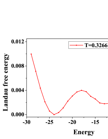
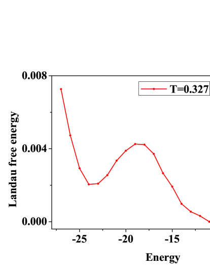
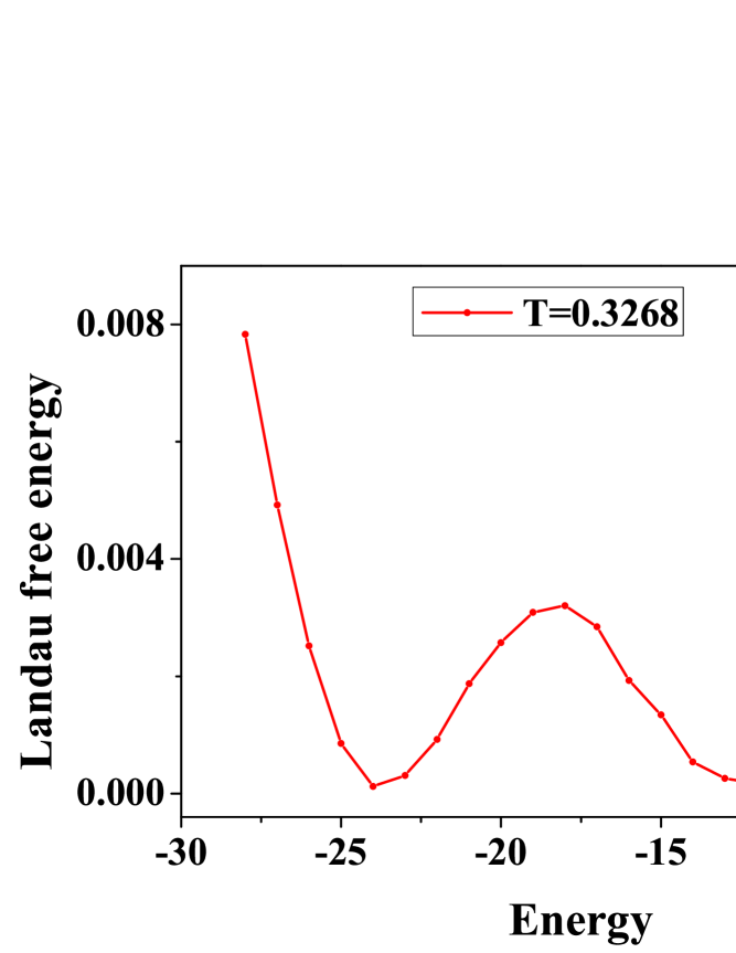
For purpose of illustration, we present the results on free energy profiles of a DNA-hairpin (hp-DNA) subjected to a constant unzipping force. DNA has two strands of equal length twisted around a common axis to form a double helix. Each strand can be considered as a chain of monomers or bases. When complementary bases at the two ends of a strand pair up, hairpin structure occurs, with a loop and stem. The structure can be closed or open. The transition from closed to open state is called denaturation or unbinding. If denaturation occurs by virtue of temperature, it is called melting. Force induced melting has been extensively studied, see [9] and the references cited therein. We present results on chain of length $110$ units. We determine the transition temperature from the peak of the specific heat profile. We take two temperatures in the neighbourhood and on either side of the transition point, to calculate free energy profiles. We have considered four site occupation, bond fluctuation model[10], on a two dimensional square lattice. For details of the simulation see [9].

We first calculate heat capacity and determine the temperature at which it is maximum. We take this as transition temperature $T_{C}$. Then we estimate the free energy versus energy profiles and these are depicted in Figures 1 - 3, for $T=T_{C}$, $T\ <\ T_{C}$, and $T\ >\ T_{C}$ respectively. It is clear the transition is first order.

6 Free Energy versus Order Parameter

Landau free energy is usually expressed as a function of order parameter $M$. Landau, Tsai, and Exler[11] defined a joint density of states $g(E,M)$ and employed it in the Wang-Landau algorithm. Let $E_{i}$ and $M_{i}$ be the energy and order parameter of the current microstate; let $E_{t}$ and $M_{t}$ denote the same quantities for the trial microstate. The acceptance probability in the Metropolis algorithm is taken as, $p={\rm min.}[1,g(E_{i},M_{i})/g(E_{t},M_{t})].$ The joint density of states is updated at every step. We also monitor the histogram $H(E,M)$. The histogram now is a two dimensional surface. When the surface becomes flat it indicates that $g(E,M)$ has converged to the true two dimensional density of states, $\widehat{\Omega}(E,M)$.

Figure 1: Variation of free energy with energy at $T\ =\ T_{C}$ and unzipping force $f=0.04$. Temperature at which the heat capacity peaks is taken as $T_{C}$. The chain length is $110$; reproduced from [9]

Figure 2: Same as Figure 1, except
$T\ <\ T_{C}$; reproduced from [9]

Figure 3: Same as Figure 1, except
$T\ >\ T_{C}$; reproduced from [9]

Obtaining a flat histogram in two dimensional space requires considerable computing time[11]. A good strategy[12] shall involve estimating the two dimensional density states in the production run, see below. The learning run is reserved, as usual, for obtaining a converged density of states in energy space only.

We assemble, in the production run, an entropic ensemble. We first un-weight the microstate and then re-weight it to a microcanonical ensemble. We estimate the joint density of states as a weighted average over the entropic ensemble. This is equivalent to averaging over a microcanonical ensemble. Thus,

$$\langle g(E_{i},M_{j})\rangle=\frac{{\displaystyle\sum_{C}\delta(E(C)-E_{i})\ \delta(M(C)-M_{j})\ g(E(C))}}{{\displaystyle\sum_{C}\delta(E(C)-E_{i})\ g(E(C))}}\hskip 12.0pt\forall\ E_{i},\ M_{j}.$$ (7)

In the above, the sum runs over all the microstates of the entropic ensemble. Having estimated the joint density of states, we calculate the Landau free energy as

$$F_{L}(M_{j},T)=-k_{B}T\ln\sum_{i}\langle g(E_{i},M_{j})\rangle\exp(-\beta E_{i})$$ (8)

where we take $T$ to be very close to the transition temperature.

6.1 Ising Spins, dsDNA and Order Parameter

Figure 4 depicts the results on Landau free energy, $F_{L}(M,T)$ versus magnetization, $M$, for a two dimensional Ising spin system.

Figure 4: Free energy versus magnetization for zero field Ising spin system; joint density of states has been calculated employing the two stage method. Two dimensional square lattice with $L=32$. The top curve is for $T\ >\ T_{C}$; the middle curve is for $T=T_{C}$; and the bottom curve is for $T\ <\ T_{C}$; reproduced from [13]

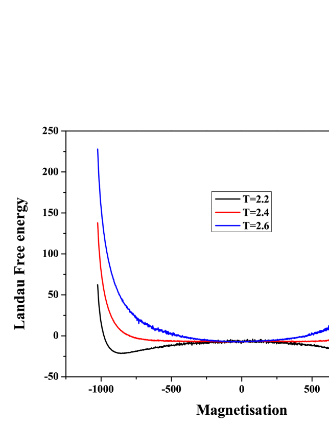
The spins are located on the vertices of a $32\times 32$ square lattice. We have estimated the joint density of states, $g(E,M)$, in the production run of Wang-Landau simulation. For details see [13]. Free energies for $T\ <\ T_{C}\ ({\rm bottom\ curve}),\ T\ =\ T_{C}\ ({\rm middle\ curve}),\ {\rm and}\ T\ >\ T_{C}\ ({\rm top\ curve})$ are shown. The transition temperature $T_{C}$ was located from the specific heat profiles.

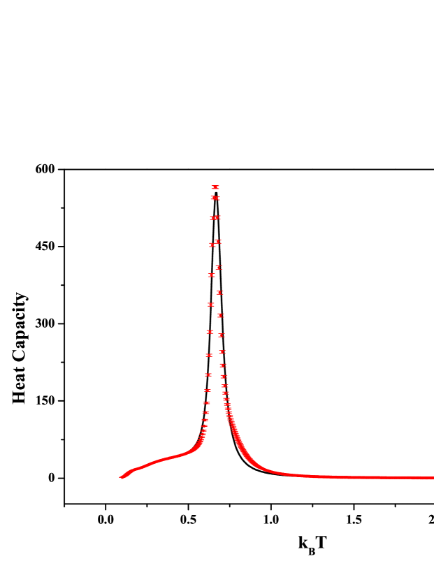
Figure 5, reproduced from [13], depicts results on variation of heat capacity with temperature, for double strand DNA. We have calculated free energy employing both the methods : (i) standard Wang-Landau algorithm in which $g(E,M)$ is obtained in the learning run and (ii) two-stage method in which $g(E,M)$ is estimated in the production run by un-weighting and re-weighting procedures. The two results agree with each other, demonstrating that the two-stage method is as good as the standard Wang-Landau sampling toward predicting mechanical properties. I must mention that the two-stage method took considerably much less computer time.

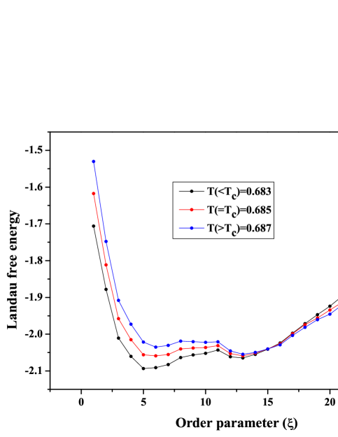
Figure 6 reproduced from [13], shows results on Landau free energy as a function of the order parameter for dsDNA. The end to end distance is taken as order parameter and is denoted by the symbol $\xi$. We have presented results at $T=T_{C}$, $T\ <\ T_{C}$ and at $T\ >\ T_{C}$. The transition is first order.

Figure 5: Heat capacity of dsDNA as a function of $T$ calculated from $g(E)$, estimated by standard Wang-Landau algorithm and from $g(E,\xi)$, obtained from the two stage method; reproduced from [13]

Figure 6: Free energy versus order parameter for a double strand DNA - dsDNA of length $80$ in the presence of unzipping force $f=0.02$. The end to end distance is taken as order parameter. Joint density of states, $g(E,\xi)$, has been calculated employing the two stage method. Top curve is for $T\ <\ T_{C}$; the middle curve is for $T=T_{C}$; the bottom curve is for T$\ >\ T_{C}$; reproduced from [13]

7 Summary

I have introduced briefly the basic principles of non-Boltzmann Monte Carlo methods. The density of states is estimated through an iterative process. Logarithm of density of states gives entropy; all other thermal properties can be estimated from entropy, employing the machinery of thermodynamics. Though a non-Boltzmann ensemble is unphysical, we can extract averages of mechanical properties, over desired physical ensembles by employing un-weighting and re-weighting techniques. Thus both thermal and mechanical properties can be estimated employing non-Boltzmann Monte Carlo simulation methods. I have illustrated the usefulness of non-Boltzmann ensemble on three systems : an hairpin DNA, Ising spins, and double stranded DNA. Results on free energy profiles at temperatures close to transition point were presented. I believe it is time we take a Non-Boltzmann Monte Carlo, as a method of first choice for simulating macroscopic systems.

References

- [1] N. Metropolis, A. W. Rosenbluth, M. N. Rosenbluth, A. H. Teller, and E. Teller 1953 J. Chem. Phys. 21 1087; see also G. Bhanot 1988 Rep. Prog. Phys. 51 429; K. P. N. Murthy 2004, Monte Carlo Methods in Statistical Physics (India : Universities Press)
- [2] K. P. N. Murthy, and V. S. S. Sastry 2005 Markov Chain Monte Carlo Methods in Statistical Physics PoS(SMPRI2005) 018
- [3] G. M. Torrie, and J. P. Valleau 1977 J. Comp. Phys. 23 187
- [4] B. A. Berg, and T. Neuhaus 1992 Phy. Rev. Lett. 68 9
- [5] J Lee 1993 Phy. Rev. Lett. 71 211; Erratum 1993 71 2353
- [6] F. Wang, and D. P. Landau 2001 Phy. Rev. Lett. 86 2050
- [7] D Jayasri, V. S. S. Sastry, and K. P. N. Murthy 2005 Phys. Rev. E 72 36702; P Poulin, F Calvo, R Antoine, M Broyer, and P Dugord 2006 Phys. Rev. E 73 56704.
- [8] Joon Chang Lee 2002 Thermal Physics : Entropy and Free Energies (Singapore : World Scientific)
- [9] M. Suman Kalyan, and K. P. N. Murthy 2015 Physica A 428 38
- [10] I. Carmesin, and K. Kremer 1988 Macromolecules 21 2819
- [11] D. P. Landau, Shan-Ho Tsai, and M. Exler 2004 Am. J. Phys. 72 1294
- [12] C. Geravais, T. Wüst, D. P. Landau, and Y. Xu 2009 J. Chem. Phys. 130 215106
- [13] M. Suman Kalyan, R. Bharath, V. S. S. Sastry, and K. P. N. Murthy 2016 J. Stat. Phys. 163 197